Brain Diffuser with Hierarchical Transformer for MCI Causality Analysis

Abstract

Effective connectivity estimation plays a crucial role in understanding the interactions and information flow between different brain regions. However, the functional time series used for estimating effective connentivity is derived from certain software, which may lead to large computing errors because of different parameter settings and degrade the ability to model complex causal relationships between brain regions. In this paper, a brain diffuser with hierarchical transformer (BDHT) is proposed to estimate effective connectivity for mild cognitive impairment (MCI) analysis. To our best knowledge, the proposed brain diffuer is the first generative model to apply diffusion models in the application of generating and analyzing multimodal brain networks. Specifically, the BDHT leverages the structural connectivity to guide the reverse processes in an efficient way. It makes the denoising process more reliable and guarantees effective connectivity estimation accuracy. To improve denoising quality, the hierarchical denoising transformer is designed to learn multi-scale features in topological space. Furthermore, the GraphConFormer block can concentrate on both global and adjacent connectivity information. By stacking the multi-head attention and graph convolutional network, the proposed model enhances structure-function complementarity and improves the ability in noise estimation. Experimental evaluations of the denoising diffusion model demonstrate its effectiveness in estimating effective connectivity. The method achieves superior performance in terms of accuracy and robustness compared to existing approaches. It can captures both unidirectal and bidirectional interactions between brain regions, providing a comprehensive understanding of the brain’s information processing mechanisms.

I Introduction

Mild cognitive impairment (MCI) is an early stage of a neurodegenerative disorder that primarily affects the brain, leading to progressive cognitive decline and memory loss[1, 2]. It typically begins with subtle memory loss and difficulty performing daily tasks and eventually leads to cognitive degradation. Understanding the underlying mechanisms and processes involved in MCI is crucial for developing effective diagnostic tools and potential treatments[3]. Effective connectivity (EC) refers to the causal influence that one brain region exerts over another, representing the flow of information and communication within the brain[4, 5]. Studying EC in patients provides valuable insights into how the disease disrupts the normal functioning of neural networks. The EC helps researchers identify the specific brain regions that are affected and how their interactions are altered[6, 7, 8]. This knowledge can aid in identifying biomarkers for early detection, tracking disease progression, and developing targeted therapeutic interventions.

The EC is distinct from functional connectivity [9], which captures statistical dependencies or correlations between brain regions of interest (ROIs) without explicitly considering the directionality or causality of the connections. It focuses on the directed causal relationships and interactions between regions, providing a more comprehensive understanding of how information is transmitted and processed in the brain. Estimating EC from functional magnetic resonance imaging (fMRI) has been a hot topic for a long time[10, 11]. Traditional methods have been designed to mine complex connectivity-based features for brain disease analysis. For example, the work in [12] applied structural equation modeling (SEM) to construct EC and evaluated the altered effective connections in schizophrenics. Rowe et al.[13] constructed EC using dynamic causal modeling (DCM) and proved its robustness in studying clinical populations for Parkinson’s disease. Liu et al.[14] modified the Granger causality models (GCM) and proposed the multivariate Granger causality analysis (mGCA) to estimate the EC among the resting state networks for MCI analysis. The other commonly used methods include the Bayesian network (BN) methods [15], the correlation analysis methods [16]. Different imaging modalities capture different aspects of brain connectivity features; integrating multimodal imaging can enhance complementarity and allow for a more complete evaluation of effective connectivity. Riedl et al.[17] proposed metabolic connectivity mapping (MCM) by combining fMRI and positron emission tomography (PET) to measure EC for brain disorder analysis. Also, Ji et al.[18] explored the combination of fMRI and diffusion tensor imaging (DTI) for learning effective connections and achieved promising results in cognitive disease diagnosis. Other works add the structural MRI[19] or the EEG data[20] to the fMRI for EC estimation. However, these methods often rely on assumptions and simplifications about the underlying neural dynamics, which can limit the ability to capture nonlinear interactions or time-varying dynamics, potentially leading to biased or incomplete estimates of effective connectivity.

The deep learning-based methods have achieved good performance in medical image analysis because of their great ability in high-level feature learning[21, 22]. Deep learning techniques perform well at modeling causal relationships between brain areas, allowing for the exploration of the deep features of fMRI[23, 24]. The study in [25] extracted the linear and nonlinear features from EEG data to identify causal relationships between brain areas with an artificial neural network. Abbasvandi et al.[26] proposed a recurrent neural network-based method to construct EC and improved disease diagnosis accuracy in both the simulation dataset and the epileptic seizures dataset. Also, the generative adversarial network (GAN)-based method is developed to learn complex data distributions for accurate EC estimation. Liu et al.[27] designed a GAN-based framework to model causal directions between pairs of brain regions from fMRI data. The work in[28] explored the combination of recurrent neural networks and GAN to estimate EC for temporal feature preservation. And Zou et al.[29] considered the non-Euclidean topological properties and constructed EC through the graph convolutional network (GCN)-based model. They captured the spatial-temporal topological relations between brain regions and achieved good performance in simulated and real datasets. The main drawbacks of current methods lie in that they heavily rely on the empirical ROI-based time series to construct EC, ignoring the manual parameter setting differences during preprocessing procedures, thus introducing large errors in EC estimation.

The straightforward way to generate ROI-based time series from 4D fMRI is to build a GAN-based model with one generator and one discriminator. When the discriminator cannot distinguish the data distribution, the optimized generator is able to map the 4D fMRI into ROI-based time series in an end-to-end manner. However, the issue of instability and mode collapse during adversarial training still has to be fully resolved [30, 31], which limits its ability to be used in this situation. Recently, denoising diffusion probabilistic models (DDPM)[32, 33] have gained significant attention in the field of machine learning and have shown promising results in various domains, including image generation[34], and audio generation[35]. The fundamental idea behind DDPM is to model the data distribution as a diffusion process, where noise is gradually transformed into the desired samples through a sequence of intermediate steps. It has shown notable benefits in generating high-quality samples with improved mode coverage and stability compared to other generative models like GANs. Therefore, we use the empirical ROI-based time series to build the forward process and use the 4D fMRI as conditioning in the reverse process. Furthermore, as the DTI provides the basic physical connection between brain regions, the DTI is coupling with the fMRI in cognitive activities[36]. Combining both of them can offer a more solid foundation for time series generation and EC estimation.

Inspired by the above observations, a brain diffuser with hierarchical transformer (BDHT) is proposed to estimate effective connectivity from 4D fMRI for MCI analysis. Specifically, considering the high dimension of 4D fMRI, anatomical knowledge is utilized to warp each 3D volume into several ROIs and compute the rough ROI-based time series. During the forward process of DDPM, the empirical ROI-based time series are added to the Gaussian noise at each step, while in the reverse process, the rough ROI-based time series and structural connectivity derived from DTI are treated as conditioning to remove the noise and generate clean samples. To capture the spatial and temporal features, the U-shaped structure-oriented transformer is designed to model the underlying relationships between distant brain regions. At last, the proposed model can estimate effective connectivity with discriminative MCI-related features from 4D fMRI in an end-to-end framework. The main contributions are summarized as follows:

• The proposed end-to-end brain diffuser framework transforms the conditioning of 4D fMRI into effective connectivity with several successive denoising steps. Particularly, the structural connectivity guides the model to learn topologtical features by capturing the relationships between adjacent brain regions, which makes the denoising process more reliable and guarantees the effective connectivity estimation to be more accurate.

• The hierarchical denoising transformer is designed to learn multi-scale features in topological space for noise removal. The related noise associated with connected ROIs can be easily removed, thus greatly improving the denoising quality. Besides, the designed transformer-based network provides a new perspective for modeling structured spatiotemporal data during the diffusive denoising process.

• By stacking the multi-head attention and graph convolutional network, the GraphConFormer block can concentrate on both global and adjacent connectivity information, which enhances structure-function complementarity and improves its ability to estimate noise.

The organization of this work is structured as follows: The main architecture of the proposed BDHT model is introduced in Section  II. In Section  III, we implement the proposed model on the public datasets and analyze the results. Section  IV shows the reliability of our results, and Section  V summarizes the main remarks of this work.

Figure 1: An overview of the conditional diffusion model, including the diffusive process (dashed line) and the denoising process (solid line). The two conditions are the rough sample $\boldsymbol{F}$ and the structural connectivity $\mathcal{G}$.

Figure 2: The framework of the proposed BDHT model. In the diffusive process, the empirical sample $\boldsymbol{H}_{0}$ is gradually transformed into the Gaussian sample $\boldsymbol{H}_{T}$ by adding noise at each successive step. In the denoising process, the rough sample $\boldsymbol{F}$ and structural connectivity $\mathcal{G}$ are input as conditioning to guide the hierarchical denoising transformer to generate the clean sample and corresponding effective connectivity.

II Method

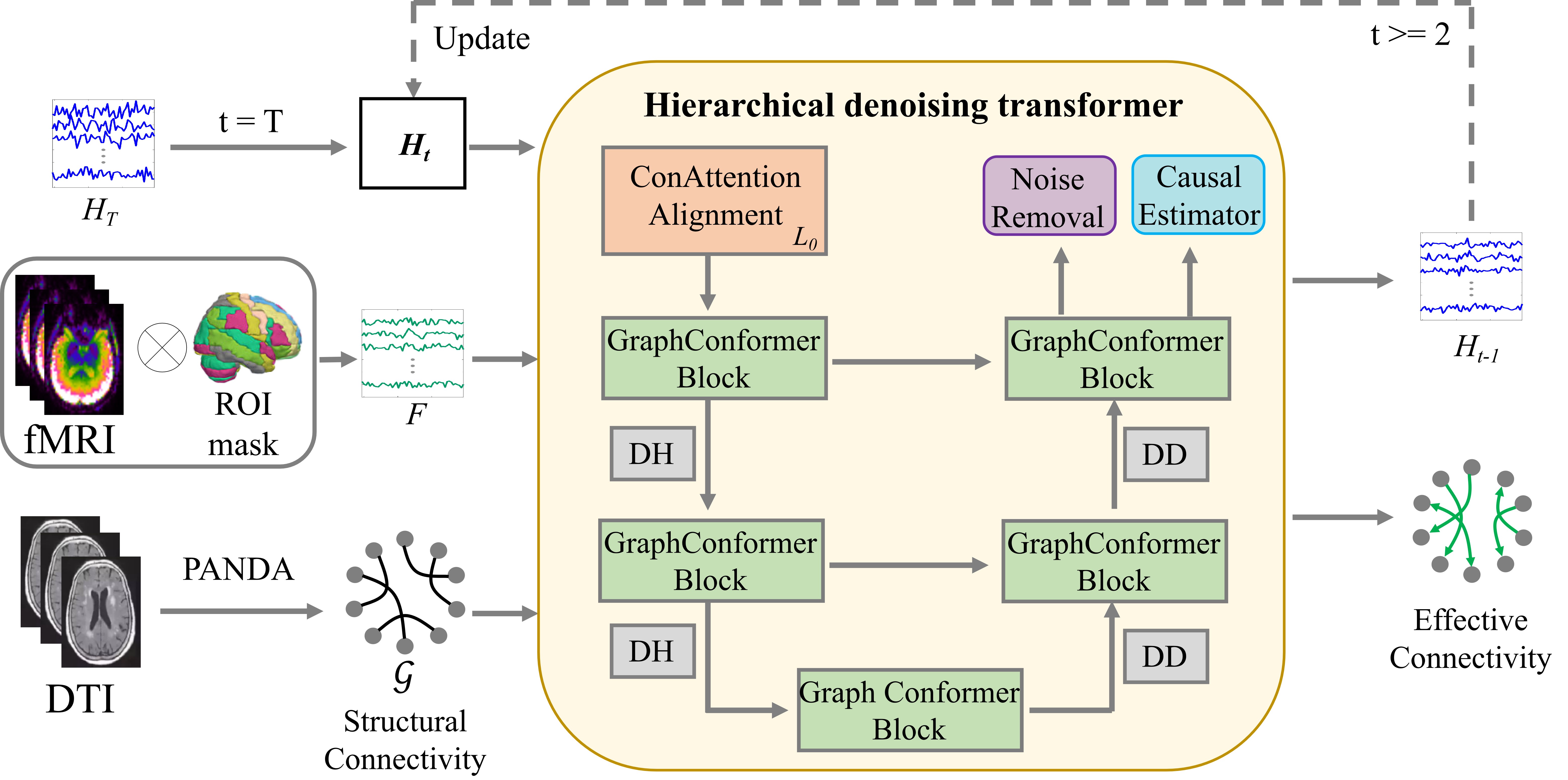
The architecture of the proposed model is shown in Fig. 2. It is based on denoising diffusion probabilistic models (DDPM). The BDHT aims to denoise the 4D fMRI into clean ROI-based time series and construct effective connectivity for MCI analysis. In the diffusive process, the empirical sample $\boldsymbol{H}_{0}$ is transformed to the Gaussian sample $\boldsymbol{H}_{T}$ by adding Gaussian noise in a series of successive steps. In the denoising process, the 4D fMRI and structural connectivity (SC) $\mathcal{G}$ are input as conditioning to guide the transformer-based network to generate the clean sample (also called clean ROI-based time series) $\boldsymbol{H}_{0}^{\prime}$ and corresponding effective connectivity $\mathbf{E}$. In the following, we first describe the basic ideas of DDPM, then present the brain structural-functional diffuser, and finally specify the detailed structure of the transformer-based denoising network.

II-A Basic ideas of DDPM

Denoising Diffusion Probabilistic Models (DDPM) is a generative modeling framework that aims to learn a Markov Chain by modeling the underlying probability distribution between Gaussian noise and clean data. Assuming the clean data distribution $q(\boldsymbol{H}_{0})$, DDPM can learn a distribution $p_{\theta}(\boldsymbol{H}_{0})$ from the Gaussian distribution to approach $q(\boldsymbol{H}_{0})$. The distribution modeling can be divided into two parts: the diffusive process and the denosing process.

In the diffusive direction, the clean sample $\boldsymbol{H}_{0}\sim q(\boldsymbol{H}_{0})$ is accumulatively added by the Gaussian noise to obtain the Gaussian sample $\boldsymbol{H}_{T}\sim\mathcal{N}(\mathbf{0},\boldsymbol{I})$ with sufficient $T(T\gg 1)$ steps. At each step, a weight is applied to the Gaussian noise to form a Markov chain. The applied weights follow a variance schedule: $\beta_{1},\beta_{2},...,\beta_{T}$. For simplification, the intermediate noisy sample $\boldsymbol{H}_{t}$ is computed from the sample at step $t-1$ with the following formulas:

$$\boldsymbol{H}_{t}=\sqrt{1-\beta_{t}}\boldsymbol{H}_{t-1}+\sqrt{\beta_{t}}\boldsymbol{\epsilon},\quad\boldsymbol{\epsilon}\sim\mathcal{N}(\mathbf{0},\boldsymbol{I})$$ (1)

$$q\left(\boldsymbol{H}_{t}\mid\boldsymbol{H}_{t-1}\right)=\mathcal{N}\left(\boldsymbol{H}_{t};\sqrt{1-\beta_{t}}\boldsymbol{H}_{t-1},\beta_{t}\boldsymbol{I}\right)$$ (2)

where $t$ ranges from $1$ to $T$, $\quad\boldsymbol{\epsilon}$ means the added Gaussian noise, $\mathcal{N}$ represents the Gaussian distribution, and $\boldsymbol{I}$ is a multivariate covariance identity matrix. $\beta_{t}\in(0,1)$ increases with the growth of time steps. After $T$ steps, the Gaussian sample $\boldsymbol{H}_{T}$ can be expressed by:

$$\boldsymbol{H}_{T}=\sqrt{\hat{\alpha}_{t}}\boldsymbol{H}_{0}+\sqrt{1-\hat{\alpha}_{t}}\boldsymbol{\epsilon}_{t}$$ (3)

here, $\alpha_{t}=1-\beta_{t},\hat{\alpha}_{t}=\prod_{j=1}^{t}\alpha_{j}$, $\boldsymbol{\epsilon}_{t}$ are sampled from the Gaussian distribution with the same size of $\boldsymbol{H}_{t}$. A large $T$ can ensure the noisy sample $\boldsymbol{H}_{t}$ approximates a standard normal distribution.

During the denoising direction, the DDPM learns a Markov chain by gradually denoising the Gaussian sample $\boldsymbol{H}_{T}$ to the clean sample $\boldsymbol{H}_{0}$. The assumptions of large $T$ and small $\beta_{t}$ guarantee adjacent samples follow the Gaussian distribution. The denoising probability from $\boldsymbol{H}_{t}$ to $\boldsymbol{H}_{t-1}$ can be defined as:

$$p_{\theta}\left(\boldsymbol{H}_{t-1}\mid\boldsymbol{H}_{t}\right)=\mathcal{N}\left(\boldsymbol{H}_{t-1};\boldsymbol{\mu}_{\theta}\left(\boldsymbol{H}_{t},t\right),\boldsymbol{\Sigma}_{\theta}\left(\boldsymbol{H}_{t},t\right)\right)$$ (4)

where the $\boldsymbol{\mu}_{\theta}(\boldsymbol{H}_{t},t)$ and $\boldsymbol{\Sigma}_{\theta}(\boldsymbol{H}_{t},t)$ are the distribution parameters that can be learned by a designed neural network. To optimize the parameterized network, the Kullback-Leibler (KL) divergence is introduced to minimize the distance between the estimated distribution $p_{\theta}(\boldsymbol{H}_{t-1}\mid\boldsymbol{H}_{t})$ and the posterior probability $q(\boldsymbol{H}_{t-1};\boldsymbol{H}_{t},\boldsymbol{H}_{0})$. After simplifying the KL formula, the Gaussian distribution parameter can be derived:

$$\boldsymbol{\mu}_{\theta}\left(\boldsymbol{H}_{t},t\right)=\frac{1}{\sqrt{\alpha_{t}}}\left(\boldsymbol{H}_{t}-\frac{\beta_{t}}{\sqrt{1-\hat{\alpha}_{t}}}\boldsymbol{\epsilon}_{\theta}\left(\boldsymbol{H}_{t},t\right)\right)$$ (5)

$$\boldsymbol{\Sigma}_{\theta}(\boldsymbol{H}_{t},t)=\frac{\left(1-\hat{\alpha}_{t-1}\right)}{\left(1-\hat{\alpha}_{t}\right)}\beta_{t}\boldsymbol{I}$$ (6)

The learnable function $\boldsymbol{\epsilon}_{\theta}$ estimates the added noise in the diffusive process, which should be removed at the denoising process. The estimated noise can be computed by the following function:

$$\operatorname*{min}_{\theta}\mathbb{E}_{\boldsymbol{H}_{0},\boldsymbol{\epsilon}_{t},t}\left\|\boldsymbol{\epsilon_{t}}-\boldsymbol{\epsilon}_{\theta}(\sqrt{\hat{\alpha}_{t}}\boldsymbol{H}_{0}+\sqrt{1-\hat{\alpha}_{t}}\boldsymbol{\epsilon}_{t},t)\right\|^{2}$$ (7)

Once the network is optimized, the Gaussian noise can be transmitted to a clean sample by removing the noise step by step.

Figure 3: The structure of the ConAttention Alignment. The inputs are the rough sample $\boldsymbol{F}$ and intermediate noisy sample $\boldsymbol{H}_{t}$, and the output is the fused feature.

Figure 4: The computing structure of the GraphConFormer block. The input is the fused feature, and the output updates the input and shares the same dimension. The $\mathcal{G}$ guides the topological feature learning in the GCN layers.

II-B Brain diffuser

The conventional DDPM is to generate clean samples from Gaussian noise without any conditions, which does not meet our task of converting 4D fMRI into effective connectivity. Therefore, we modify the DDPM and propose the brain functional diffuser by adding the 4D fMRI as a condition in the denoising direction. Besides, considering the topological properties can provide rich information about the estimated noise in the denoising process, we add another condition, which is the structural connectivity $\mathcal{G}$. As shown in Fig. 1, the diffusive process of the brain functional diffuser is the same as Eq.( 1), while the denoising process can be expressed as follows:

$$p_{\theta}\left(\boldsymbol{H}_{t-1}\mid\boldsymbol{H}_{t},\boldsymbol{F},\mathcal{G}\right)=$$ (8)

$$\mathcal{N}\left(\boldsymbol{H}_{t-1};\boldsymbol{\mu}_{\theta}\left(\boldsymbol{H}_{t},t\mid\boldsymbol{F},\mathcal{G}\right),\boldsymbol{\Sigma}_{\theta}\left(\boldsymbol{H}_{t},t\mid\boldsymbol{F},\mathcal{G}\right)\right)$$

$$p_{\theta}\left(\boldsymbol{H}_{0:T}\mid\boldsymbol{F},\mathcal{G}\right)=p\left(\boldsymbol{H}_{T}\right)\prod_{t=1}^{T}p_{\theta}\left(\boldsymbol{H}_{t-1}\mid\boldsymbol{H}_{t},\boldsymbol{F},\mathcal{G}\right)$$ (9)

We define the network of causal estimator as $\boldsymbol{\phi}_{\theta}$ consisting of two multilayer perceptron (MLP) layers. The structure in the transformer-based network are denoted as $\boldsymbol{\epsilon}_{\theta}$. The predicted noisy sample $\boldsymbol{H}_{t-1}^{\prime}$, the reconstructed noisy sample $\hat{\boldsymbol{H}}_{t-1}$ and the effective connectivity $\mathbf{E}$ are defined as:

$$\boldsymbol{H}_{t-1}^{\prime}= \sqrt{\hat{\alpha}_{t-1}}\left(\frac{\boldsymbol{H}_{t}-\sqrt{1-\hat{\alpha}_{t}}\cdot\boldsymbol{\epsilon}_{\theta}\left(\boldsymbol{H}_{t},t\mid\boldsymbol{F},\mathcal{G}\right)}{\sqrt{\hat{\alpha}_{t}}}\right)$$ (10)

$$+\sqrt{1-\hat{\alpha}_{t-1}}\cdot\boldsymbol{\epsilon}_{\theta}\left(\boldsymbol{H}_{t},t\mid\boldsymbol{F},\mathcal{G}\right)$$

$$\hat{\boldsymbol{H}}_{t-1},\mathbf{E}=\boldsymbol{\phi}_{\theta}(\boldsymbol{H}_{t},\boldsymbol{\epsilon}_{\theta},t)$$ (11)

During the optmization, we sample $(\boldsymbol{H}_{0},\boldsymbol{F},\mathcal{G})\sim q(\boldsymbol{H}_{0},\boldsymbol{F},\mathcal{G})$ from truth data distribution. The denoising process can be trained by the following objective function:

$$\mathcal{L}(\theta)= \mathbb{E}_{\boldsymbol{H}_{t},\boldsymbol{\epsilon}_{t},t}\left\|\boldsymbol{\epsilon_{t}}-\boldsymbol{\epsilon}_{\theta}\left(\boldsymbol{H}_{t},t\mid\boldsymbol{F},\mathcal{G}\right)\right\|^{2}$$ (12)

$$+\mathbb{E}_{\boldsymbol{H}_{t-1},\boldsymbol{\epsilon}_{\theta},t}\left\|\boldsymbol{H}_{t-1}-\hat{\boldsymbol{H}}_{t-1}\right\|^{2}+\frac{\omega}{N*N}\left\|\mathbf{E}\right\|$$

Thousands of sampling steps lead to slow denoising computation; we reduce the sampling steps by deviding the whole $T$ steps into several sub-steps. Assuming the new total sampling steps are $T_{n}$ and the sampling interval is $m$, we can define the new sampling step formula: $j=floor(i/m)+1,i\in{1,2,...,T},j\in{1,2,...,T_{n}}$.

II-C Hierarchical denoising transformer

The inputs of the denoising network are the intermediate noisy sample $\boldsymbol{H}_{t}\in\mathbb{R}^{N\times q}$, the rough (conditional) sample $\boldsymbol{F}\in\mathbb{R}^{N\times q}$, and the structural connectivity $\mathcal{G}\in\mathbb{R}^{N\times N}$. Note that $N$ is the number of ROIs, and $q$ is the dimension of each sample. The $\boldsymbol{F}$ is obtained by pixel multiplication between the 4D fMRI and the anatomical ROI mask. The $\mathcal{G}$ is estimated from diffusion tensor imaging (DTI) by the GRETNA software. During the denoising computation, there are three main modules, including the conditional attention alignment (ConAttention alignment), the graph convolutional transformer (GraphConFormer), the noise removal and causal estimator. After the denoising is complete, the classifier is adopted to evaluate the discriminability of the generated effective connectivities.

II-C1 Conditional attention alignment

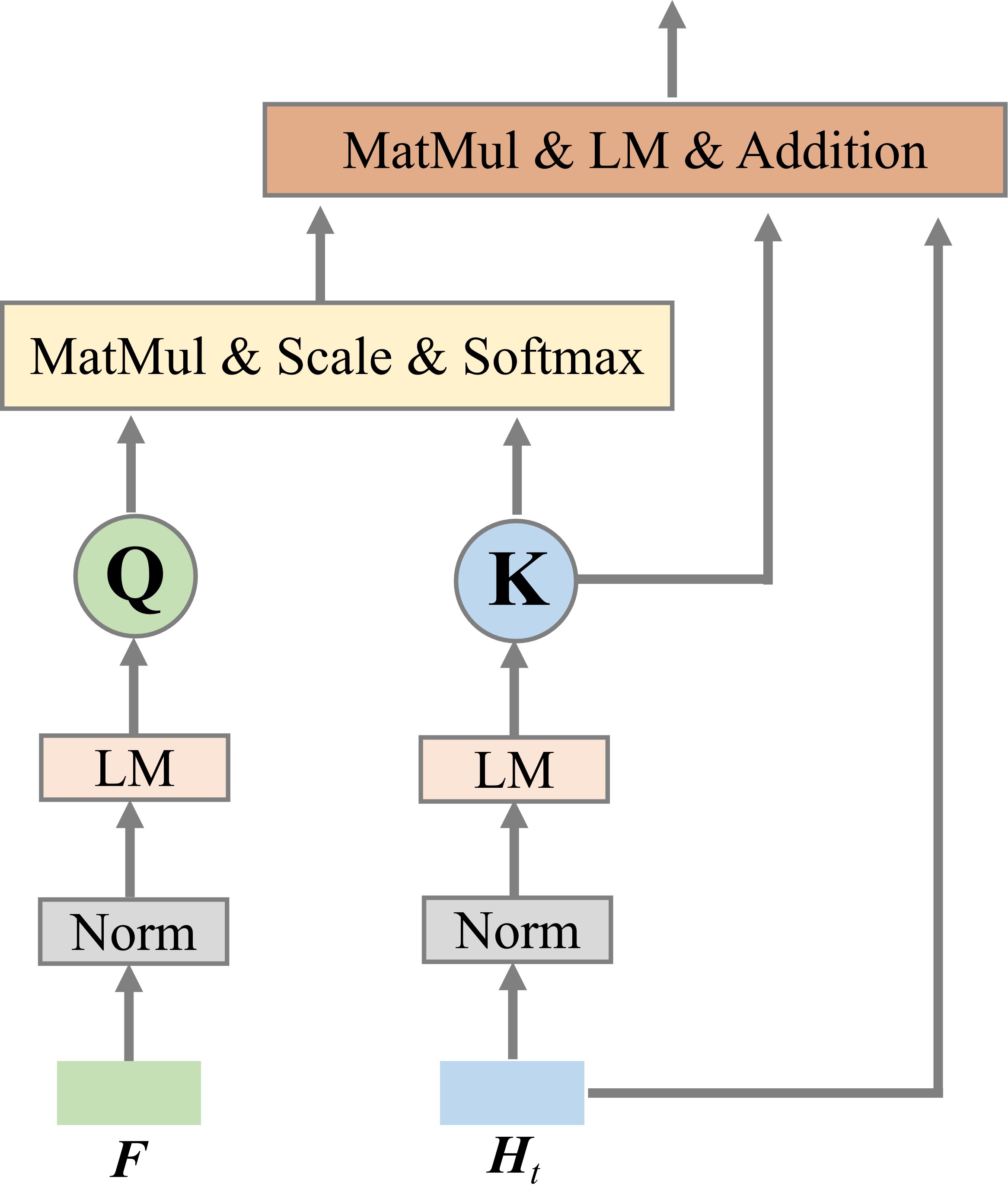
The current approach of fusing the conditional sample and the intermediate noisy sample is to concatenate them [37], which leads to high dimensions in our study. As shown in Fig. 3, we design one-layer linear mapping (LM) to obtain the Query ($\boldsymbol{Q}$) and Key ($\boldsymbol{K}$). An attention layer is applied to the $\boldsymbol{Q}$ and $\boldsymbol{V}$ to compute the fused feature $\boldsymbol{H}_{t}^{ConAttention}$. The fused ROI-based feature can be well aligned between the conditional sample $\boldsymbol{F}$ and the intermediate noisy sample $\boldsymbol{H}_{t}$, enhancing the signal and suppressing the noise. The calculation process is as follows:

$$\boldsymbol{Q}=LM_{1}(Norm(\boldsymbol{F})),\boldsymbol{K}=LM_{2}(Norm(\boldsymbol{H}_{t}))$$ (13)

$$\mathcal{X}=\operatorname{softmax}\left(\frac{\boldsymbol{Q}\boldsymbol{K}^{T}}{\sqrt{q}}\right)\boldsymbol{K}$$ (14)

$$\boldsymbol{H}_{t}^{ConAttention}=LM_{3}(\mathcal{X})+\boldsymbol{H}_{t}$$ (15)

After $L_{0}$ ConAttention blocks, the fused feature $\boldsymbol{H}_{t}^{ConAttention}$ has the same length as $\boldsymbol{H}_{t}$.

II-C2 Graph convolutional transformer

To learn multi-scale features in topological space for noise removal, we design a U-shaped structure consisting of GraphConFormer, dimension halving (DH), and dimension doubling (DD). As shown in Fig. 4, the GraphConFormer block stacks multi-head attention networks and graph convolutional networks for extracting both global and adjacent connectivity information. To be specific, the fused feature $\boldsymbol{H}_{t}^{ConAttention}$ first passes the spatial multi-head attention (SMA), then passes the temporal multi-head attention (TMA). The spatiotemporal feature can be greatly enhanced. Finally, the structural connectivity $\mathcal{G}$ guides the model to learn topological features by using two graph convolutional networks (GCN). The detailed computation steps are given as follows:

$$\Gamma_{1}=ReLU(SMA(Norm(\Gamma_{0})))+\Gamma_{0}$$ (16)

$$\Gamma_{2}=ReLU(TMA(Norm(\Gamma_{1})))+\Gamma_{1}$$ (17)

$$\boldsymbol{H}_{t}^{GraphConFormer}=ReLU(GCN(ReLU(GCN(\Gamma_{2},\mathcal{G}))))+\Gamma_{2}$$ (18)

here, the input $\Gamma_{0}$ represents the $\boldsymbol{H}_{t}^{ConAttention}$ in the first layer, and the variable $\Gamma_{1}$ and $\Gamma_{2}$ represent the operations of SMA and TMA, respectively. For SMA, the sequence is the dimension of each ROI feature, and the heads are set as $h_{s}$; for TMA, the sequence is all the ROI features of each element along the dimension direction, and the heads are set as $h_{t}$. The output $\boldsymbol{H}_{t}^{GraphConFormer}$ has the same size as $\Gamma_{0}$.

The DH module is a GCN layer, which reduces the feature dimension. For the first DH block, the input dimension is $q$, and the output dimension is $q/2$. The DD module is also a GCN layer for dimension increase. For the first DD block, the input dimension is $q/4$, and the output dimension is $q/2$. The arrow between GraphConFormer blocks means adding operations.

Algorithm 1 Training of brain diffuser

0:  $\boldsymbol{H}_{0}$: empirical sample
     $\boldsymbol{F}$: conditional sample
     $T$: number of diffusion steps
     $\mathcal{G}$: structural connectivity

0:  Noise removal function $\boldsymbol{\epsilon}_{\theta}$ and causal estimator $\boldsymbol{\phi}_{\theta}$

1:  initial variance schedle $\beta_{i},i=1,2,...,T$; $\omega=2.5$

2:  repeat

3:     $t\sim Uniform({1,2,...,T})$,$\boldsymbol{H}_{0}\sim q(\boldsymbol{H}_{0})$

4:     Sample $\boldsymbol{\epsilon}_{t}\sim\mathcal{N}(\mathbf{0},\boldsymbol{I})$

5:     Calculate the diffusive sample $\boldsymbol{H}_{t}$ using Eq.( 3)

6:     Take gradient descent step on $\nabla_{\theta}\mathcal{L}(\theta)$

7:  until converged

II-C3 Noise removal and Causal estimator

The aforementioned GraphConFormer outputs the estimated noise $\boldsymbol{\epsilon}_{\theta}\left(\boldsymbol{H}_{t},t\mid\boldsymbol{F},\mathcal{G}\right)$, we utilize the Eq.( 10) to calculate the denoised sample. The output at $t=0$ clean sample is defined as $\boldsymbol{H}_{0}^{\prime}$, which is similar to $\boldsymbol{H}_{0}$.

In the causal estimator, we explore the causal relations between any pair of brain regions. After the concatenation of $\boldsymbol{\epsilon}_{\theta}$ and $\boldsymbol{H}_{t}$ pass two layers of MLP, the structural equation model (SEM) is adopted to model the signal flow from one brain region to another. Assuming $x_{i}$ represents the $i$-th ROI time series, all brain regions exerting effects on the $i$-th ROI can be expressed by:

$$x_{i}^{\prime}=\sum_{j=1}^{N}\mathbf{E}_{ji}x_{j}+\varepsilon_{i}$$ (19)

where $\varepsilon_{i}$ represents the error when reconstructing the target signal. The calculated matrix $\mathbf{E}$ is asymmetric with a size of $N\times N$. The diagonal elements of $\mathbf{E}$ are zeros because we don’t consider the causal effects of the brain region itself. The $x_{i}^{\prime}$ is the $i$-th row vector of the intermediate noisy sample $\boldsymbol{H}_{t-1}$. The estimated effective connectivity matrices are sent into the classifier for classification evaluation.

The pseudo-code of the training and sampling processes is displayed in Algorithm 1 and Algorithm 2.

Algorithm 2 Sampling of brain diffuser

0:  $\boldsymbol{F}$: conditional sample
     $T$: number of diffusion steps
     $\mathcal{G}$: structural connectivity
     $\boldsymbol{\epsilon}_{\theta}$: noise estimation function
     $\boldsymbol{\phi}_{\theta}$: causal estimation function

0:  Clean sample $\boldsymbol{H}_{0}^{\prime}$ and effective connectivity $\mathbf{E}$

1:  Sample $\boldsymbol{\epsilon}_{t}\sim\mathcal{N}(\mathbf{0},\boldsymbol{I})$

2:  for $t=T$ to $1$ do

3:     Calculate the intermediate sample $\boldsymbol{H}_{t-1}^{\prime}$ using Eq.( 10)
     by taking $\boldsymbol{F}$ and $\mathcal{G}$ as conditions

4:     Update the effective connectivity $\mathbf{E}$ using Eq.( 11)

5:  end for

6:  Return $\boldsymbol{H}_{0}^{\prime}$ and $\mathbf{E}$

III Experiments

III-A Datasets

Our study was conducted on the publicly available Alzheimer’s Disease Neuroimaging Initiative (ADNI) dataset. We selected the same number of subjects for each category, including significant memory concern (SMC), early mild cognitive impairment (EMCI), late mild cognitive impairment (LMCI), and normal control (NC). The total number of subjects is 240, scanned with both functional magnetic resonance imaging (fMRI) and DTI. The male-to-female ratio is nearly balanced.

The fMRI scans were performed by Siemens using the following parameters: a repetition time (TR) of 3.0 s and an echo-planar imaging (EPI) sequence consisting of 197 volumes. There are two preprocessing approaches for the fMRI data, both of which require the anatomical automatic labeling (AAL90) atlas [38] for computing region of interest (ROI)-based time series. The first approach involves using the GRETNA software to obtain the functional time series, which serves as the empirical sample $\boldsymbol{H}_{0}$ in our proposed model. The specific computation steps using GRETNA [39] are described in the work by Zuo et al. [40]. The second approach is our study, which utilizes the standard atlas file $aal.nii$ to divide each fMRI volume into 90 brain regions and average the voxel values within each region. We removed the first 10 volumes and obtained the rough sample $\boldsymbol{F}\in\mathbb{R}^{90\times 187}$. The DTI scanning directions range from 6 to 126. To preprocess the DTI, we utilized the PANDA toolbox [41] and obtained the structural connectivity with dimensions of $90\times 90$.

Figure 5: An example of denoising conditional sample at different steps for the $1$st ROI in AAL90 atlas. The top arrow is the conditional time series calculated by the non-parametric dot product, and the bottom row is the empirical time series computed by the GRETNA software.

Figure 6: Comparison of reconstructing time series using different methods.

Figure 7: Prediction performance of binary classification tasks on the ADNI dataset. Three competing models are compared with our model.

III-B Training Settings and Evaluation Metrics

In our experiment, the proposed model aims to transform the four-dimensional fMRI into ROI-based time series and an effective connectivity network. We set the total diffusing steps as $100$, and the sampling parameters are set as: $T_{n}=10,m=10$. The $L_{0}$ is 2. The sparsity constraint parameter $\omega$ is $2.5$. The code is written with Python tools and runs on the Ubuntu 18.04 system. The total epochs are 800. The Adam optimizer is adopted to update the model’s weights with a learning rate of 0.001.

The results are evaluated using a 5-fold cross-validation strategy. For the reconstruction task, we utilize the mean absolute error (MAE) and the root mean square error (RMSE) to estimate the model’s performance. For the classification tasks (i.e., NC vs. EMCI, NC vs. LMCI), the four commonly used metrics are considered: the prediction accuracy (ACC), the patient sensitivity (SEN), the healthy specificity (SPE), and the area under the receiver operating characteristic curve (AUC).

III-C Denoised and Prediction Results

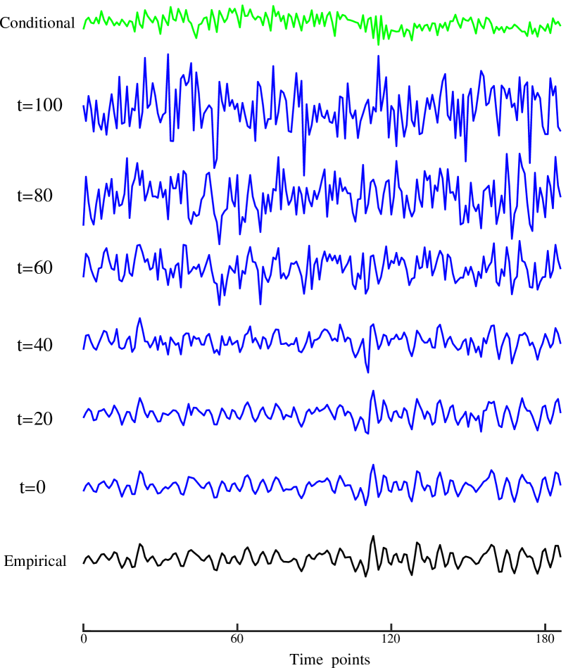
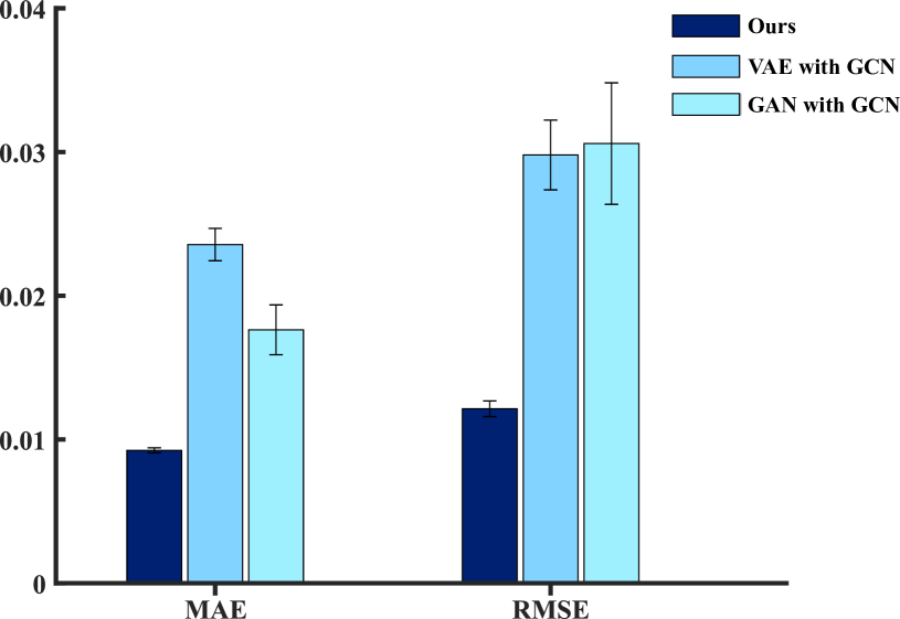
The output of the proposed model is the denoised time series and the effective connectivity. We evaluated the performance of the generated time series. The details of generating one ROI-based time series by our model are displayed in Fig. 5. As the time steps decrease, the Gaussian noise is gradually transformed into a clean time series. We select two other generative frameworks for comparison, including the variational autoencoder (VAE) and the generative adversarial network (GAN). These two frameworks accept both SC and rough time series by designing graph convolutional networks (GCN). As shown in Fig. 6, the VAE-based or GAN-based models have larger reconstructed errors, while our model achieves the minimum mean value for MAE and RMSE with 0.0092 and 0.0121, respectively. The standard error of our model is also lower than that of the other two models.

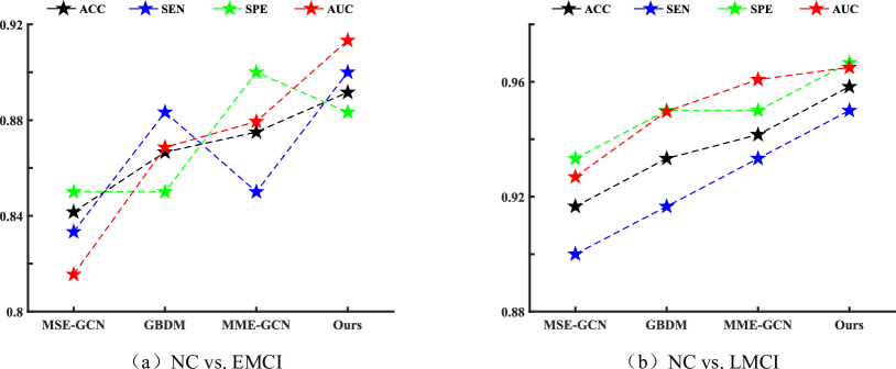
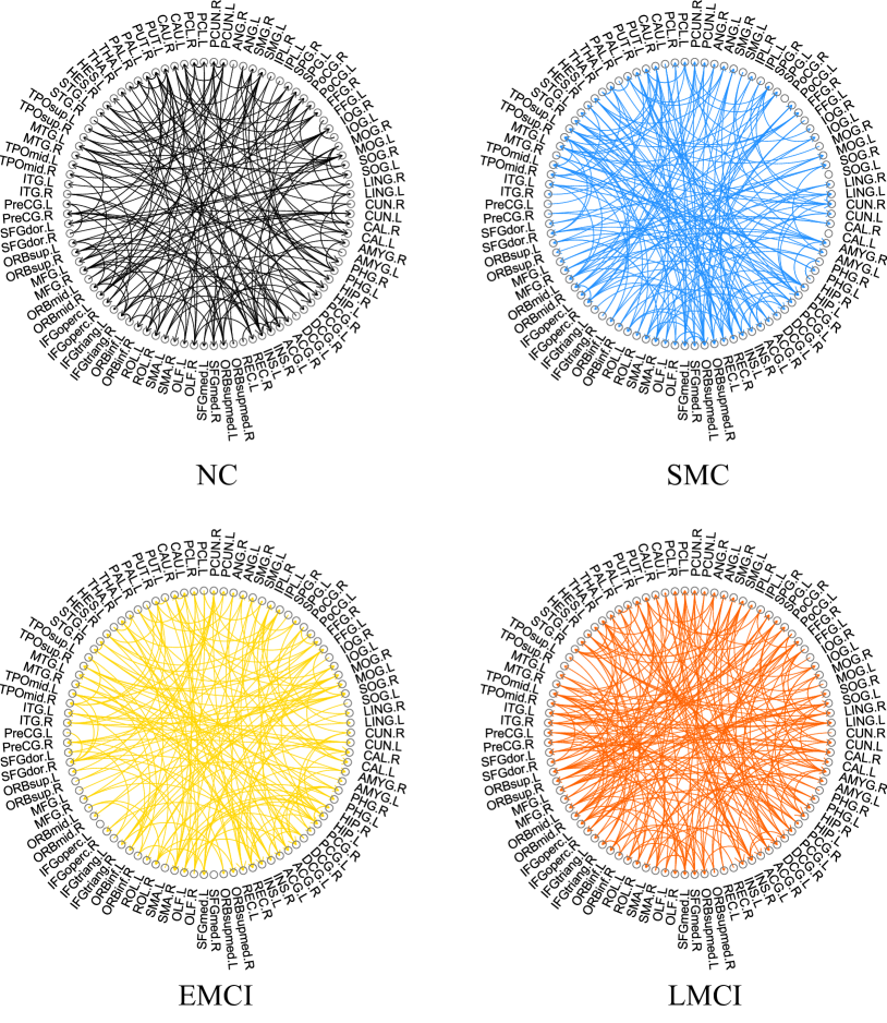
To estimate the quality of generated ECs, we conducted two binary classification experiments. Three other related methods are introduced to fuse empirical functional time series and structural connectivity and generate structural-functional connectivities (SFCs). We compare the classification performance using ECs and SFCs with the same BrainNetCNN classifier [42]. These three methods are (1) the MSE-GCN method [43], (2) the GBDM method [44], and (3) the MME-GCN method [45]. The classification results are displayed in Fig. 7. Examples of geneated ECs are shown in Fig. 8. Among the four methods, our model achieves the best classification performance with an ACC value of 89.16%, SEN value of 90.0%, and AUC value of 91.33% for NC vs. EMCI. For NC vs. LMCI, the best values of ACC, SEN, SPE, and AUC are 95.83%, 95.0%, 96.67%, and 96.50%, respectively. This may indicate that causal connections carry much more MCI-related information than undirected connections.

Figure 8: Examples of the effective connectivities generated at four different stages. The 90 brain regions are arranged counterclockwise.

Figure 9: Visualization of the top five enhanced and diminished effective connections from NC to SMC. The green color means enhanced effective connections, and the purple color means diminished effective connections.

Figure 10: Visualization of the top five enhanced and diminished effective connections from SMC to EMCI.

Figure 11: Visualization of the top five enhanced and diminished effective connections from EMCI to LMCI.

III-D Analysis of Effective Connectivity

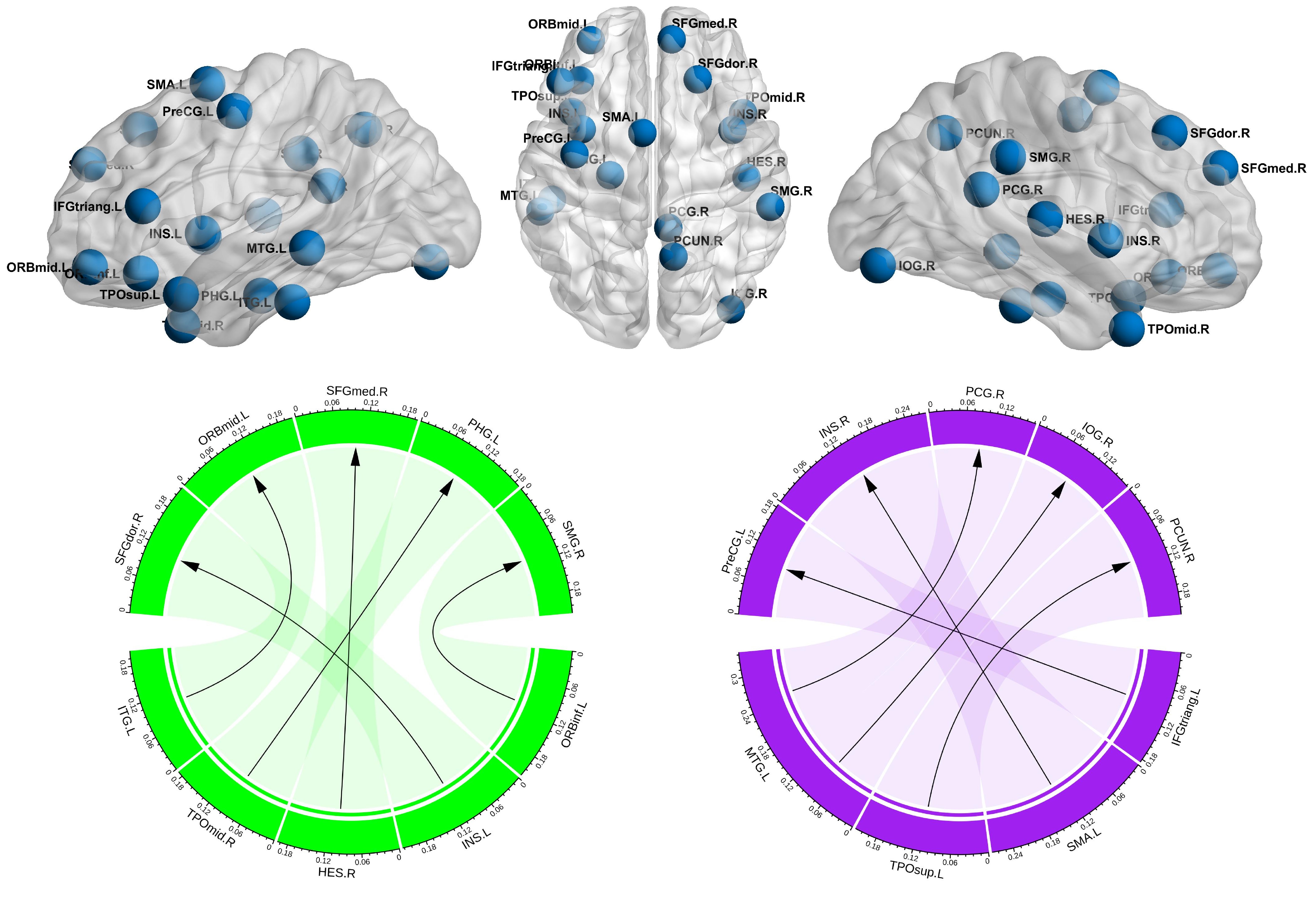
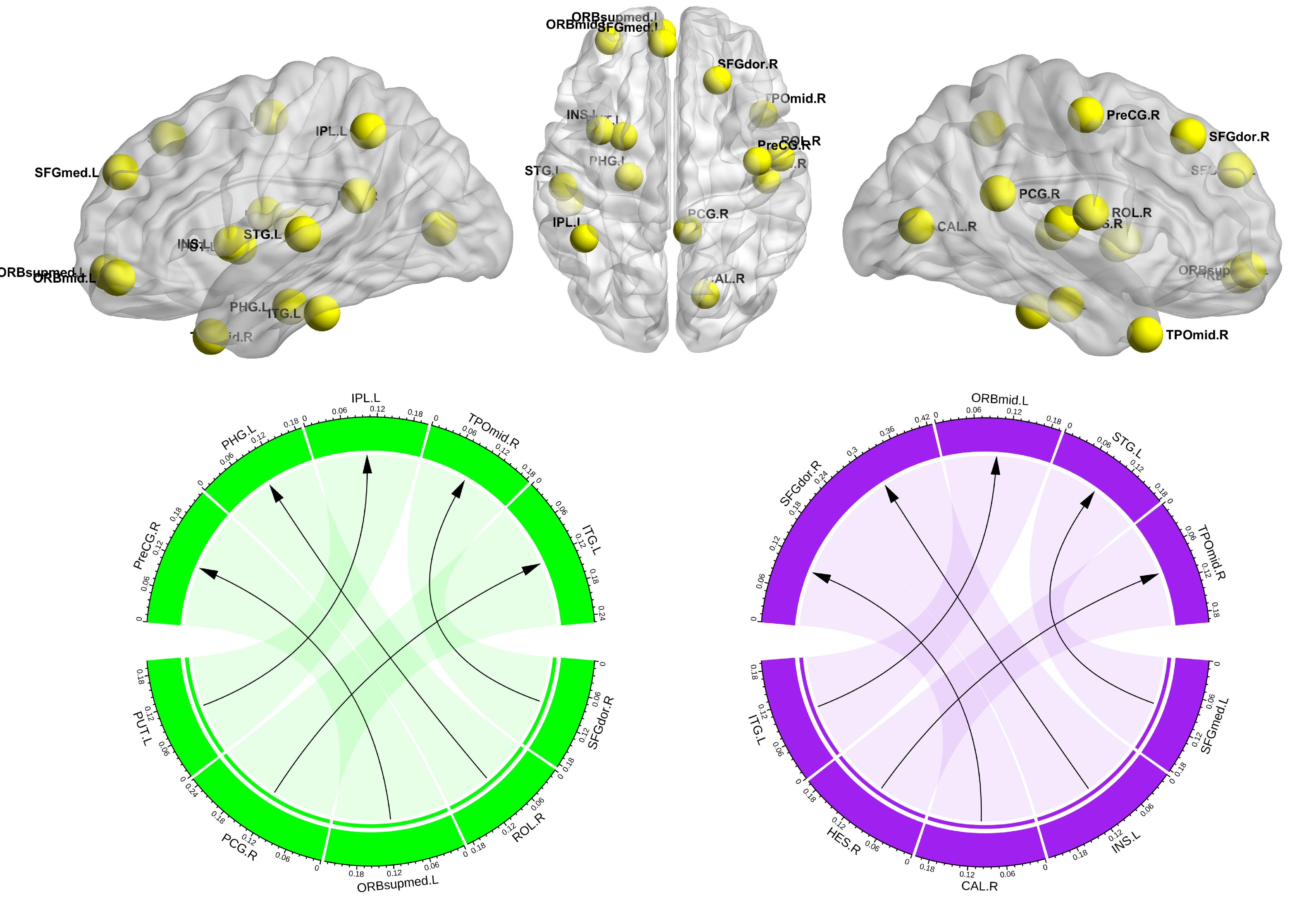
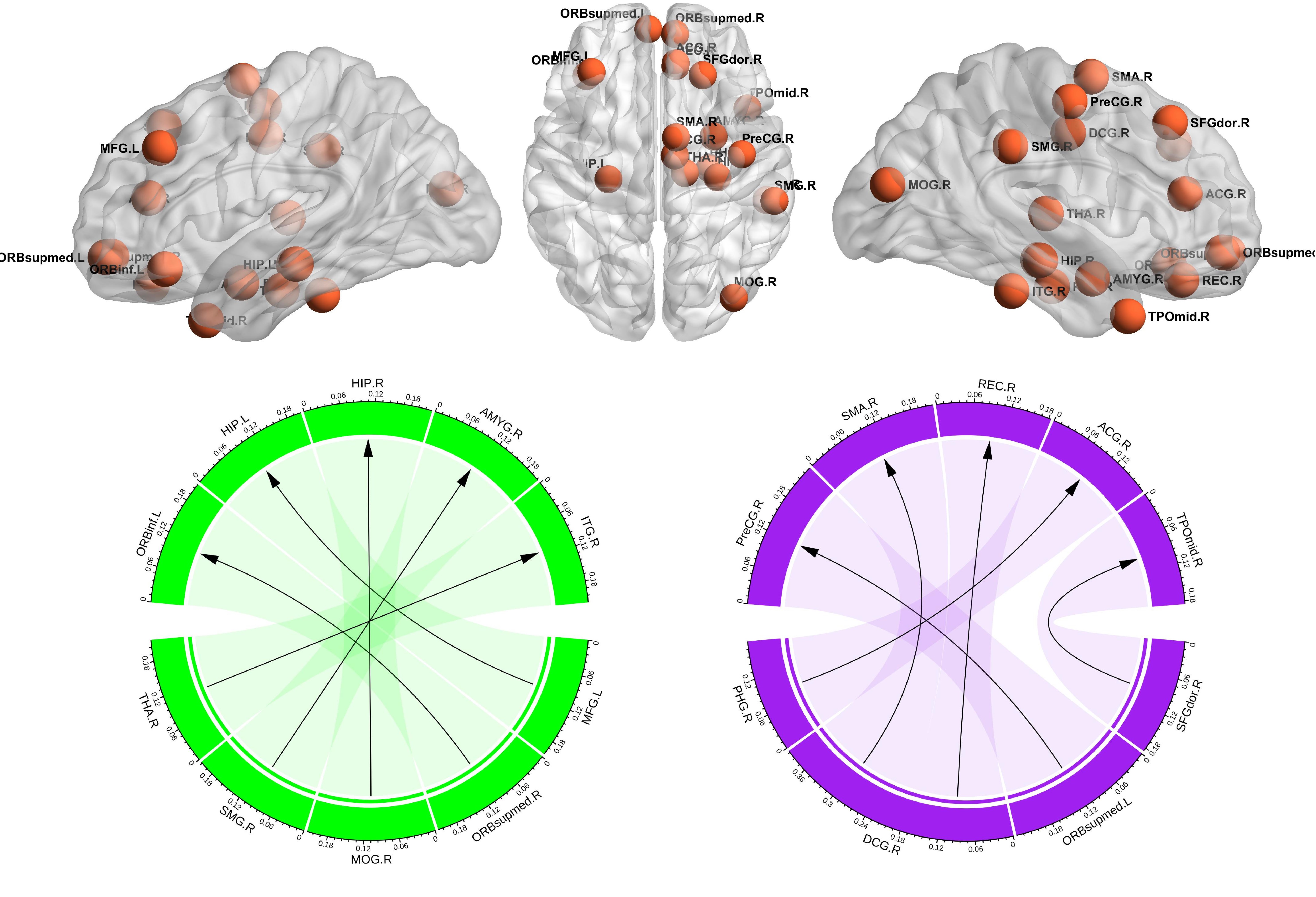
During disease progression, the effective connections can show abnormal patterns. We call these patterns as altered effective connections. As mentioned in the previous studies [46], we compute the mean EC for each group (i.e., NC, SMC, EMCI, and LMCI). The altered effective connectivity can be calculated by dividing the latter stage by the former stage. The positive value in the altered effective connectivity means enhanced effective connection, and the negative value means diminished effective connection. To obtain the largest altered strength of effective connections, we sort the positive and negative values, respectively. As shown in Fig. 9, the top part displays the distribution of these connection-related brain regions, and the bottom part is the strength of altered connections. The top 10 altered effective connections from NC to SMC are INS.L $\rightarrow$ SFGdor.R, ORBinf.L $\rightarrow$ SMG.R, ITG.L $\rightarrow$ ORBmid.L, HES.R $\rightarrow$ SFGmed.R, TPOmid.R $\rightarrow$ PHG.L, SMA.L $\rightarrow$ INS.R, TPOsup.L $\rightarrow$ PCUN.R, IFGtriang.L $\rightarrow$ PreCG.L, MTG.L $\rightarrow$ PCG.R, and MTG.L $\rightarrow$ IOG.R. The top ten altered effective connections from SMC to EMCI are shown in Fig. 10. These effective connections are SFGdor.R $\rightarrow$ TPOmid.R, ROL.R $\rightarrow$ PHG.L, ORBsupmed.L $\rightarrow$ PreCG.R, PCG.R $\rightarrow$ ITG.L, PUT.L $\rightarrow$ IPL.L, SFGmed.L $\rightarrow$ STG.L, INS.L $\rightarrow$ SFGdor.R, CAL.R $\rightarrow$ SFGdor.R, HES.R $\rightarrow$ TPOmid.R, and ITG.L $\rightarrow$ ORBmid.L. Fig. 11 shows the top ten altered effective connections between EMCI and LMCI groups, including MFG.L $\rightarrow$ HIP.L, ORBsupmed.R $\rightarrow$ ORBinf.L, MOG.R $\rightarrow$ HIP.R, SMG.R $\rightarrow$ AMYG.R, THA.R $\rightarrow$ ITG.R, SFGdor.R $\rightarrow$ TPOmid.R, ORBsupmed.L $\rightarrow$ PreCG.R, DCG.R $\rightarrow$ SMA.R, DCG.R $\rightarrow$ REC.R, and PHG.R $\rightarrow$ ACG.R.

TABLE I: Top five bidirectional altered connections for three scenarios.

	ROIs index	ROI names
NC vs. SMC	19, 30	SMA.L $\leftrightarrow$ INS.R
	15, 64	ORBinf.L $\leftrightarrow$ SMG.R
	1, 13	PreCG.L $\leftrightarrow$ IFGtriang.L
	21, 69	OLF.L $\leftrightarrow$ PCL.L
	26, 60	ORBsupmed.R $\leftrightarrow$ SPG.R
SMC vs. EMCI	36, 89	PCG.R $\leftrightarrow$ ITG.L
	4, 29	SFGdor.R $\leftrightarrow$ INS.L
	2, 25	PreCG.R $\leftrightarrow$ ORBsupmed.L
	5, 20	ORBsup.L $\leftrightarrow$ SMA.R
	27, 31	REC.L $\leftrightarrow$ ACG.L
EMCI vs. LMCI	4, 88	SFGdor.R $\leftrightarrow$ TPOmid.R
	37, 61	HIP.L $\leftrightarrow$ IPL.L
	20, 78	SMA.R $\leftrightarrow$ THA.R
	2, 25	PreCG.R$\leftrightarrow$ ORBsupmed.L
	68, 87	PCUN.R $\leftrightarrow$ TPOmid.L

Figure 12: Visualization of the top ROI-related effective connections that are calculated by aggregating the altered connection strength for each brain region. The three brain regions are PoCG.R, ORBmid.R, and PHG.L for NC vs. SMC, SMC vs. EMCI, and EMCI vs. LMCI, respectively.

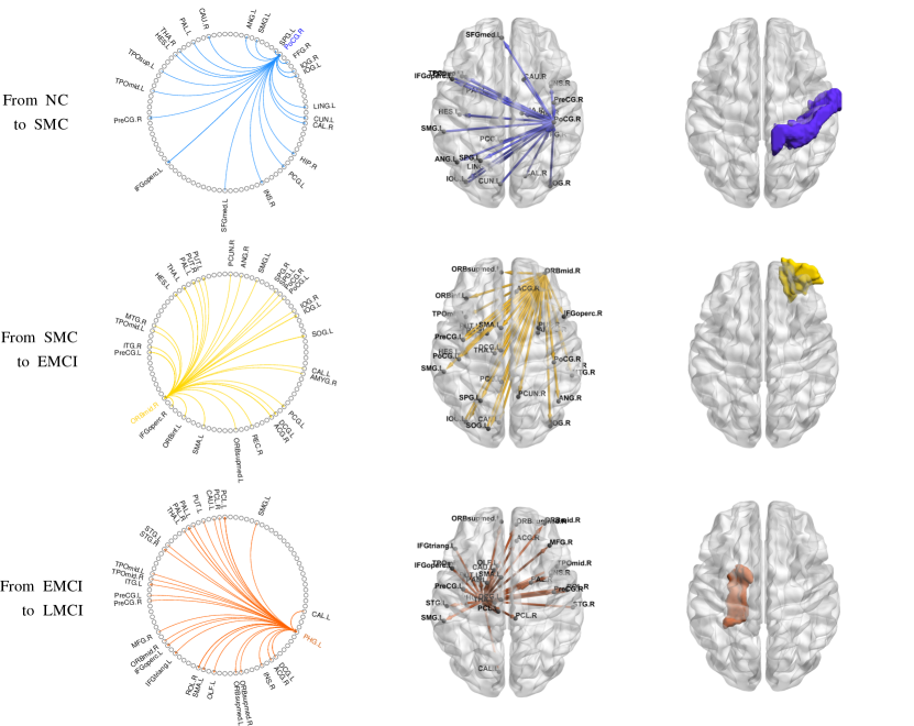
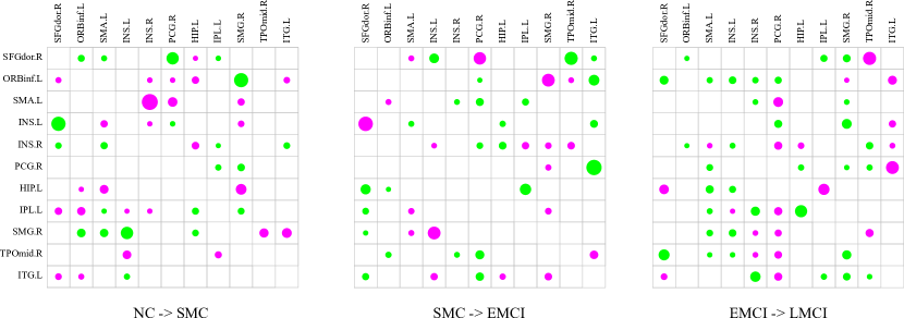
To analyze the important brain regions that contribute most to MCI, we ignore the sign of each altered connection and sum the altered connection strength for each brain region. After sorting the summed ROI strength in descending order, the top five ROIs are the potential biomarkers in the MCI pregression. Fig. 12 shows the top brain region and its related effective connections during three scenarios. The top five ROIs for NC vs. SMC are PoCG.R, AMYG.L, ROL.R, LING.R and FFG.L. From SMC to EMCI, the five important ROIs are ORBmid.R, SMG.R, IFGoperc.L, SOG.R and ORBsup.R. The five important ROIs between EMCI and LMCI groups are PHG.L, SFGdor.L, SMG.L, SOG.L and IFGtriang.L. These identified ROIs are partly consistent with previous studies [47, 48]. Furthermore, we analyze the bidirectionally altered connections among different groups. For each pair of ROIs, we sum their absolute values and sort these values for all pairs. The calculated top five bidirectional altered connections are shown in Tab. I. To compare these connection characteristics at different stages, we select two pairs of bidirectional altered connections for each scenario and present them in Fig. 13. The values below 0.1 are not displayed. The number of enhanced effective connections (green color) tends to increase compared with that of the diminished connections (magenta color) as the disease progresses. This characteristic can be explained by the compensatory mechnism at MCI stage [49]. We select one pair of altered connections for each scenario and obtain six brain regions. Fig. 14 shows the effective connection characteristics changing among six brain regions during the disease progression. For visualization convenience, all brain regions are projected onto the sagittal plane. Compared with NC, more enhanced connections are founded at MCI-related stages than at SMC.

Figure 13: The effective connections of the paired ROIs that have bidirectional altered connections. Effective connection strengths lower than 0.1 are not considered. The magenta and green colors represent the diminished and enhanced effective connections, respectively. The circle size indicates the relative connection strength.

Figure 14: Display of effective connections among six representative ROIs by projecting them onto the sagittal plane of the brain at four different stages The black arrow means the original effective connections at NC, and the colored arrow means altered effective connections.

III-E Ablation Study

The proposed BDHT model can denoise the 4D fMRI into effective connectivity. To prove the effectiveness of the designed network structure, we studied two variants of BDHT to evaluate the prediction performance of NC vs. EMCI. One variant (BDHT w/o U-shape) removes the U-shaped structure in the BDHT, which means the DD and DH are included in our model; the other variant (BDHT w/o Transformer) removes the SMA and TMA in the GraphConFormer block. The prediction results are listed in Tab. II. The BDHT without the transformer shows the worst classification performance, which drops at least 4 percentage points on the ACC value. While removing the U-shape structure in the BDHT drops about 2 percent on the ACC calculation, It probably means that the spatiotemporal features carry much more MCI-related information than the multi-scale features.

TABLE II: Impact of the BDHT structure on the prediction performance.(%)

	ACC	SEN	SPE	AUC
BDHT w/o U-shape	85.00	86.67	83.33	85.14
BDHT w/o Tranformer	87.50	86.67	88.33	87.67
proposed BDHT	89.17	90.00	88.33	91.33

IV Discussion

The motivation of the proposed model is to denoise the 4D fMRI into ROI-based time series and effective connectivity. Previous studies obtained the ROI-based time series from 4D fMRI by using certain software. A few of them focus on combining the ROI-based time series using a deep learning model. Our model is methodologically feasible. The ROI mask of the AAL90 atlas is a prior knowledge that can partition a three-dimensional volume into 90 parts for each time point. This step has no learnable parameters. The mean pixel value of each ROI can generate rougth ROI-based time series. This rough sample has unknown noise compared with the empirical sample (using the software toolbox), which can be treated as a condition in the reverse direction of DDPM. Furthermore, the structural connectivity can be used to extract topological characteristics in the reverse process. Meanwhile, the causal relationships between brain regions can be explored using the SEM method. Fig. 6 shows that the proposed BDHT has the potential to replace the software toolbox in preprocessing functional MRI.

The experimental results show important unidirectional and bidirectional altered connections. The frequently appearing brain regions are Superior frontal gyrus dorsolateral, Inferior frontal gyrus triangular part, Superior frontal gyrus medial orbital, Parahippocampal gyrus, Supramarginal gyrus, and Temporal pole middle temporal gyrus. These brain regions are reported to be correlated with MCI [50, 51, 52, 53]. For example, the Parahippocampal gyrus has main functions include creating memories and recalling visual scenes. Damage to this gyrus in patients disrupts the memory-related neural circuit and causes cognitive decline. The Supramarginal gyrus controls language expression in the neural center; abnormal effective connections with it cause language dysfunction and severely affect social activities. Fig. 14 gives the effective connection changing characteristics among six representative ROIs from NC to LMCI. The SMC stage shows one enhanced and one diminished effective connection compared with the NC stage. As the progression comes at EMCI, three more effective connections are emerging. When LMCI occurs, one more effective connection gets lost. This phenomenon can be explained by the following: SMC shows slight changes in the brain network; EMCI compensates the whole brain network for daily activities; and LMCI causes further damage to the brain functions. Therefore, much more attention should be paid to the EMCI stage.

The main limitation of this work is that it ignores the dynamic changes in characteristics during cognitive progression. As the functional time series carries much more underlying information about the MCI, constructing dynamic effective connectivities can uncover the pathological mechanisms of the MCI and make the results more interpretable. In the future, we will bridge the dynamic causal relationships among brain regions for clinical applications.

V Conclusion

This paper proposes a brain diffuser with hierarchical transformer (BDHT) to construct effective connectivity from four-dimensional fMRI for MCI analysis. The BDHT leverages structural connectivity to guide the denoising process through the brain diffuser. The designed U-shape structure learns multi-scale features in topological space for denoising enhancement. Meanwhile, the GraphConFormer block, consisting of the multi-head attention and graph convolutional network, improves the structure-function fusion effect and boosts noise removal ability. The proposed model was evaluated on the ADNI dataset and achieves superior denoising quality and prediction performance than related models. The BDHT can identify important brain regions and effective connections for MCI diagnosis. The identified unidirectional and bidirectional effective connections may have the potential to be biomarkers for MCI treatment.

Data Availability Statement

The experimental dataset in this article is readily available in the [Alzheimer’s Disease Neuroimaging Initiative](https://adni.loni.usc.edu).

References

- [1] R. Gupta and N. Sen, “Traumatic brain injury: a risk factor for neurodegenerative diseases,” Reviews in the Neurosciences, vol. 27, no. 1, pp. 93–100, 2016.
- [2] B. Lei, E. Liang, M. Yang, P. Yang, F. Zhou, E.-L. Tan, Y. Lei, C.-M. Liu, T. Wang, X. Xiao et al., “Predicting clinical scores for alzheimer’s disease based on joint and deep learning,” Expert Systems with Applications, vol. 187, p. 115966, 2022.
- [3] M. A. Myszczynska, P. N. Ojamies, A. M. Lacoste, D. Neil, A. Saffari, R. Mead, G. M. Hautbergue, J. D. Holbrook, and L. Ferraiuolo, “Applications of machine learning to diagnosis and treatment of neurodegenerative diseases,” Nature Reviews Neurology, vol. 16, no. 8, pp. 440–456, 2020.
- [4] G. Deshpande, P. Santhanam, and X. Hu, “Instantaneous and causal connectivity in resting state brain networks derived from functional mri data,” Neuroimage, vol. 54, no. 2, pp. 1043–1052, 2011.
- [5] H.-J. Park, K. J. Friston, C. Pae, B. Park, and A. Razi, “Dynamic effective connectivity in resting state fmri,” NeuroImage, vol. 180, pp. 594–608, 2018.
- [6] Y. Zhong, L. Huang, S. Cai, Y. Zhang, K. M. von Deneen, A. Ren, J. Ren, A. D. N. Initiative et al., “Altered effective connectivity patterns of the default mode network in alzheimer’s disease: an fmri study,” Neuroscience letters, vol. 578, pp. 171–175, 2014.
- [7] M. Scherr, L. Utz, M. Tahmasian, L. Pasquini, M. J. Grothe, J. P. Rauschecker, T. Grimmer, A. Drzezga, C. Sorg, and V. Riedl, “Effective connectivity in the default mode network is distinctively disrupted in alzheimer’s disease–simultaneous resting-state fdg-pet/fmri study,” Human brain mapping, vol. 42, no. 13, pp. 4134–4143, 2021.
- [8] Z. Xia, T. Zhou, S. Mamoon, A. Alfakih, and J. Lu, “A structure-guided effective and temporal-lag connectivity network for revealing brain disorder mechanisms,” IEEE Journal of Biomedical and Health Informatics, 2023.
- [9] B. Lei, S. Yu, X. Zhao, A. F. Frangi, E.-L. Tan, A. Elazab, T. Wang, and S. Wang, “Diagnosis of early alzheimer’s disease based on dynamic high order networks,” Brain imaging and behavior, vol. 15, pp. 276–287, 2021.
- [10] G. Deshpande, X. Hu, R. Stilla, and K. Sathian, “Effective connectivity during haptic perception: a study using granger causality analysis of functional magnetic resonance imaging data,” Neuroimage, vol. 40, no. 4, pp. 1807–1814, 2008.
- [11] K. Friston, “Causal modelling and brain connectivity in functional magnetic resonance imaging,” PLoS biology, vol. 7, no. 2, p. e1000033, 2009.
- [12] R. Schlösser, T. Gesierich, B. Kaufmann, G. Vucurevic, S. Hunsche, J. Gawehn, and P. Stoeter, “Altered effective connectivity during working memory performance in schizophrenia: a study with fmri and structural equation modeling,” Neuroimage, vol. 19, no. 3, pp. 751–763, 2003.
- [13] J. B. Rowe, L. E. Hughes, R. A. Barker, and A. M. Owen, “Dynamic causal modelling of effective connectivity from fmri: are results reproducible and sensitive to parkinson’s disease and its treatment?” Neuroimage, vol. 52, no. 3, pp. 1015–1026, 2010.
- [14] Z. Liu, L. Bai, R. Dai, C. Zhong, H. Wang, Y. You, W. Wei, and J. Tian, “Exploring the effective connectivity of resting state networks in mild cognitive impairment: an fmri study combining ica and multivariate granger causality analysis,” in 2012 Annual International Conference of the IEEE Engineering in Medicine and Biology Society. IEEE, 2012, pp. 5454–5457.
- [15] X. Wu, X. Wen, J. Li, and L. Yao, “A new dynamic bayesian network approach for determining effective connectivity from fmri data,” Neural Computing and Applications, vol. 24, pp. 91–97, 2014.
- [16] N. Xu, R. N. Spreng, and P. C. Doerschuk, “Initial validation for the estimation of resting-state fmri effective connectivity by a generalization of the correlation approach,” Frontiers in neuroscience, vol. 11, p. 271, 2017.
- [17] V. Riedl, L. Utz, G. Castrillón, T. Grimmer, J. P. Rauschecker, M. Ploner, K. J. Friston, A. Drzezga, and C. Sorg, “Metabolic connectivity mapping reveals effective connectivity in the resting human brain,” Proceedings of the National Academy of Sciences, vol. 113, no. 2, pp. 428–433, 2016.
- [18] J. Ji, J. Liu, A. Zou, and A. Zhang, “Acoec-fd: Ant colony optimization for learning brain effective connectivity networks from functional mri and diffusion tensor imaging,” Frontiers in Neuroscience, vol. 13, p. 1290, 2019.
- [19] S. Chiang, M. Guindani, H. J. Yeh, Z. Haneef, J. M. Stern, and M. Vannucci, “Bayesian vector autoregressive model for multi-subject effective connectivity inference using multi-modal neuroimaging data,” Human brain mapping, vol. 38, no. 3, pp. 1311–1332, 2017.
- [20] A. R. Anwar, M. Muthalib, S. Perrey, A. Galka, O. Granert, S. Wolff, U. Heute, G. Deuschl, J. Raethjen, and M. Muthuraman, “Effective connectivity of cortical sensorimotor networks during finger movement tasks: a simultaneous fnirs, fmri, eeg study,” Brain topography, vol. 29, pp. 645–660, 2016.
- [21] S. Wang, X. Wang, Y. Shen, B. He, X. Zhao, P. W.-H. Cheung, J. P. Y. Cheung, K. D.-K. Luk, and Y. Hu, “An ensemble-based densely-connected deep learning system for assessment of skeletal maturity,” IEEE Transactions on Systems, Man, and Cybernetics: Systems, vol. 52, no. 1, pp. 426–437, 2020.
- [22] S. Hu, W. Yu, Z. Chen, and S. Wang, “Medical image reconstruction using generative adversarial network for alzheimer disease assessment with class-imbalance problem,” in 2020 IEEE 6th international conference on computer and communications (ICCC). IEEE, 2020, pp. 1323–1327.
- [23] N. Talebi, A. M. Nasrabadi, and I. Mohammad-Rezazadeh, “Estimation of effective connectivity using multi-layer perceptron artificial neural network,” Cognitive neurodynamics, vol. 12, pp. 21–42, 2018.
- [24] Y. Wang, Y. Wang, and Y. W. Lui, “Generalized recurrent neural network accommodating dynamic causal modeling for functional mri analysis,” NeuroImage, vol. 178, pp. 385–402, 2018.
- [25] N. Talebi, A. M. Nasrabadi, I. Mohammad-Rezazadeh, and R. Coben, “Ncreann: Nonlinear causal relationship estimation by artificial neural network; applied for autism connectivity study,” IEEE transactions on medical imaging, vol. 38, no. 12, pp. 2883–2890, 2019.
- [26] Z. Abbasvandi and A. M. Nasrabadi, “A self-organized recurrent neural network for estimating the effective connectivity and its application to eeg data,” Computers in biology and medicine, vol. 110, pp. 93–107, 2019.
- [27] J. Liu, J. Ji, G. Xun, L. Yao, M. Huai, and A. Zhang, “Ec-gan: inferring brain effective connectivity via generative adversarial networks,” in Proceedings of the AAAI Conference on Artificial Intelligence, vol. 34, no. 04, 2020, pp. 4852–4859.
- [28] J. Ji, J. Liu, L. Han, and F. Wang, “Estimating effective connectivity by recurrent generative adversarial networks,” IEEE Transactions on Medical Imaging, vol. 40, no. 12, pp. 3326–3336, 2021.
- [29] A. Zou, J. Ji, M. Lei, J. Liu, and Y. Song, “Exploring brain effective connectivity networks through spatiotemporal graph convolutional models,” IEEE Transactions on Neural Networks and Learning Systems, 2022.
- [30] S. Hu, Y. Shen, S. Wang, and B. Lei, “Brain mr to pet synthesis via bidirectional generative adversarial network,” in Medical Image Computing and Computer Assisted Intervention–MICCAI 2020: 23rd International Conference, Lima, Peru, October 4–8, 2020, Proceedings, Part II 23. Springer, 2020, pp. 698–707.
- [31] S. Wang, Z. Chen, S. You, B. Wang, Y. Shen, and B. Lei, “Brain stroke lesion segmentation using consistent perception generative adversarial network,” Neural Computing and Applications, vol. 34, no. 11, pp. 8657–8669, 2022.
- [32] J. Ho, A. Jain, and P. Abbeel, “Denoising diffusion probabilistic models,” Advances in Neural Information Processing Systems, vol. 33, pp. 6840–6851, 2020.
- [33] A. Q. Nichol and P. Dhariwal, “Improved denoising diffusion probabilistic models,” in International Conference on Machine Learning. PMLR, 2021, pp. 8162–8171.
- [34] A. Lugmayr, M. Danelljan, A. Romero, F. Yu, R. Timofte, and L. Van Gool, “Repaint: Inpainting using denoising diffusion probabilistic models,” in Proceedings of the IEEE/CVF Conference on Computer Vision and Pattern Recognition, 2022, pp. 11 461–11 471.
- [35] Y. Leng, Z. Chen, J. Guo, H. Liu, J. Chen, X. Tan, D. Mandic, L. He, X. Li, T. Qin et al., “Binauralgrad: A two-stage conditional diffusion probabilistic model for binaural audio synthesis,” Advances in Neural Information Processing Systems, vol. 35, pp. 23 689–23 700, 2022.
- [36] H.-J. Park and K. Friston, “Structural and functional brain networks: from connections to cognition,” Science, vol. 342, no. 6158, p. 1238411, 2013.
- [37] L. Guo, C. Wang, W. Yang, S. Huang, Y. Wang, H. Pfister, and B. Wen, “Shadowdiffusion: When degradation prior meets diffusion model for shadow removal,” in Proceedings of the IEEE/CVF Conference on Computer Vision and Pattern Recognition, 2023, pp. 14 049–14 058.
- [38] N. Tzourio-Mazoyer, B. Landeau, D. Papathanassiou, F. Crivello, O. Etard, N. Delcroix, B. Mazoyer, and M. Joliot, “Automated anatomical labeling of activations in spm using a macroscopic anatomical parcellation of the mni mri single-subject brain,” Neuroimage, vol. 15, no. 1, pp. 273–289, 2002.
- [39] J. Wang, X. Wang, M. Xia, X. Liao, A. Evans, and Y. He, “Gretna: a graph theoretical network analysis toolbox for imaging connectomics,” Frontiers in human neuroscience, vol. 9, p. 386, 2015.
- [40] Q. Zuo, L. Lu, L. Wang, J. Zuo, and T. Ouyang, “Constructing brain functional network by adversarial temporal-spatial aligned transformer for early ad analysis,” Frontiers in Neuroscience, vol. 16, p. 1087176, 2022.
- [41] Z. Cui, S. Zhong, P. Xu, Y. He, and G. Gong, “Panda: a pipeline toolbox for analyzing brain diffusion images,” Frontiers in human neuroscience, vol. 7, p. 42, 2013.
- [42] J. Kawahara, C. J. Brown, S. P. Miller, B. G. Booth, V. Chau, R. E. Grunau, J. G. Zwicker, and G. Hamarneh, “Brainnetcnn: Convolutional neural networks for brain networks; towards predicting neurodevelopment,” NeuroImage, vol. 146, pp. 1038–1049, 2017.
- [43] S. Yu, S. Wang, X. Xiao, J. Cao, G. Yue, D. Liu, T. Wang, Y. Xu, and B. Lei, “Multi-scale enhanced graph convolutional network for early mild cognitive impairment detection,” in Medical Image Computing and Computer Assisted Intervention–MICCAI 2020: 23rd International Conference, Lima, Peru, October 4–8, 2020, Proceedings, Part VII 23. Springer, 2020, pp. 228–237.
- [44] L. Zhang, L. Wang, J. Gao, S. L. Risacher, J. Yan, G. Li, T. Liu, D. Zhu, A. D. N. Initiative et al., “Deep fusion of brain structure-function in mild cognitive impairment,” Medical image analysis, vol. 72, p. 102082, 2021.
- [45] L. Liu, Y.-P. Wang, Y. Wang, P. Zhang, and S. Xiong, “An enhanced multi-modal brain graph network for classifying neuropsychiatric disorders,” Medical Image Analysis, vol. 81, p. 102550, 2022.
- [46] Q. Zuo, B. Lei, N. Zhong, Y. Pan, and S. Wang, “Brain structure-function fusing representation learning using adversarial decomposed-vae for analyzing mci,” arXiv preprint arXiv:2305.14404, 2023.
- [47] B. Lei, N. Cheng, A. F. Frangi, E.-L. Tan, J. Cao, P. Yang, A. Elazab, J. Du, Y. Xu, and T. Wang, “Self-calibrated brain network estimation and joint non-convex multi-task learning for identification of early alzheimer’s disease,” Medical image analysis, vol. 61, p. 101652, 2020.
- [48] X. Song, F. Zhou, A. F. Frangi, J. Cao, X. Xiao, Y. Lei, T. Wang, and B. Lei, “Graph convolution network with similarity awareness and adaptive calibration for disease-induced deterioration prediction,” Medical Image Analysis, vol. 69, p. 101947, 2021.
- [49] Z. Qi, X. Wu, Z. Wang, N. Zhang, H. Dong, L. Yao, and K. Li, “Impairment and compensation coexist in amnestic mci default mode network,” Neuroimage, vol. 50, no. 1, pp. 48–55, 2010.
- [50] X. Wang, X. Cui, C. Ding, D. Li, C. Cheng, B. Wang, and J. Xiang, “Deficit of cross-frequency integration in mild cognitive impairment and alzheimer’s disease: A multilayer network approach,” Journal of Magnetic Resonance Imaging, vol. 53, no. 5, pp. 1387–1398, 2021.
- [51] S. J. Chung, Y. J. Kim, J. H. Jung, H. S. Lee, B. S. Ye, Y. H. Sohn, Y. Jeong, and P. H. Lee, “Association between white matter connectivity and early dementia in patients with parkinson disease,” Neurology, vol. 98, no. 18, pp. e1846–e1856, 2022.
- [52] S.-Y. Lin, C.-P. Lin, T.-J. Hsieh, C.-F. Lin, S.-H. Chen, Y.-P. Chao, Y.-S. Chen, C.-C. Hsu, and L.-W. Kuo, “Multiparametric graph theoretical analysis reveals altered structural and functional network topology in alzheimer’s disease,” NeuroImage: Clinical, vol. 22, p. 101680, 2019.
- [53] M. Bozzali, G. J. Parker, L. Serra, K. Embleton, T. Gili, R. Perri, C. Caltagirone, and M. Cercignani, “Anatomical connectivity mapping: a new tool to assess brain disconnection in alzheimer’s disease,” Neuroimage, vol. 54, no. 3, pp. 2045–2051, 2011.