Conformalised data synthesis with statistical quality guarantees

Abstract

With the proliferation of ever more complicated Deep Learning architectures, data synthesis is a highly promising technique to address the demand of data-hungry models. However, reliably assessing the quality of a ‘synthesiser’ model’s output is an open research question with significant associated risks for high-stake domains. To address this challenge, we have designed a unique confident data synthesis algorithm that introduces statistical confidence guarantees through a novel extension of the Conformal Prediction framework. We support our proposed algorithm with theoretical proofs and an extensive empirical evaluation of five benchmark datasets. To show our approach’s versatility on ubiquitous real-world challenges, the datasets were carefully selected for their variety of difficult characteristics: low sample count, class imbalance and non-separability, and privacy-sensitive data. In all trials, training sets extended with our confident synthesised data performed at least as well as the original, and frequently significantly improved Deep Learning performance by up to +65% F₁-score.

MSC Classification]68T37

1 Introduction

Specialised and data-hungry Deep Learning implementations are increasingly faced with small and unrepresentative datasets, a well-established challenge in the literature [1, 2, 3]. Unfortunately, collecting more data to increase the sample size is difficult in many real-world applications. Prohibitors include the high cost of data collection, low data availability, and the lack of expertise in ground-truth labelling.

Data synthesis is a highly sophisticated approach to combat small datasets. Improving on techniques that tweak and remix existing samples (e.g., data resampling, randomisation, and augmentation), data synthesis generates entirely new and unseen examples based on the original data [4]. Similarly to classification, synthesis relies on accurately modelling the data’s distribution to extrapolate plausible new feature vectors [5]. In Deep Learning, these synthesised samples may be included in the training set to improve model generalisation and, consequently, prediction performance. A major challenge and open research question with existing data synthesis techniques, such as Generative Neural Networks (GANs), is how to measure the quality of their synthetic data. Evaluating a generator model’s distributional fit is fundamentally difficult because there is no inherent quality metric for previously unseen data.

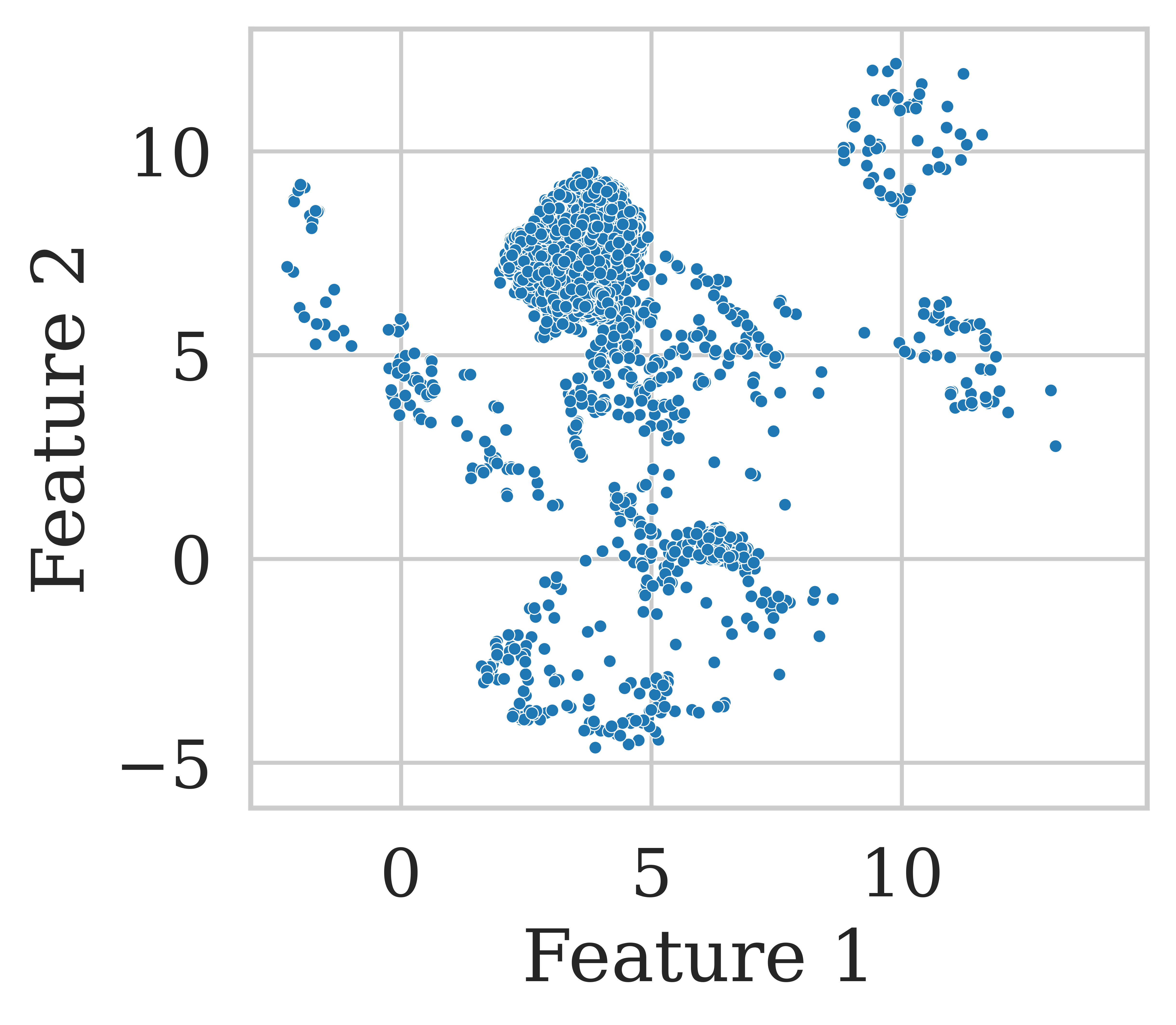
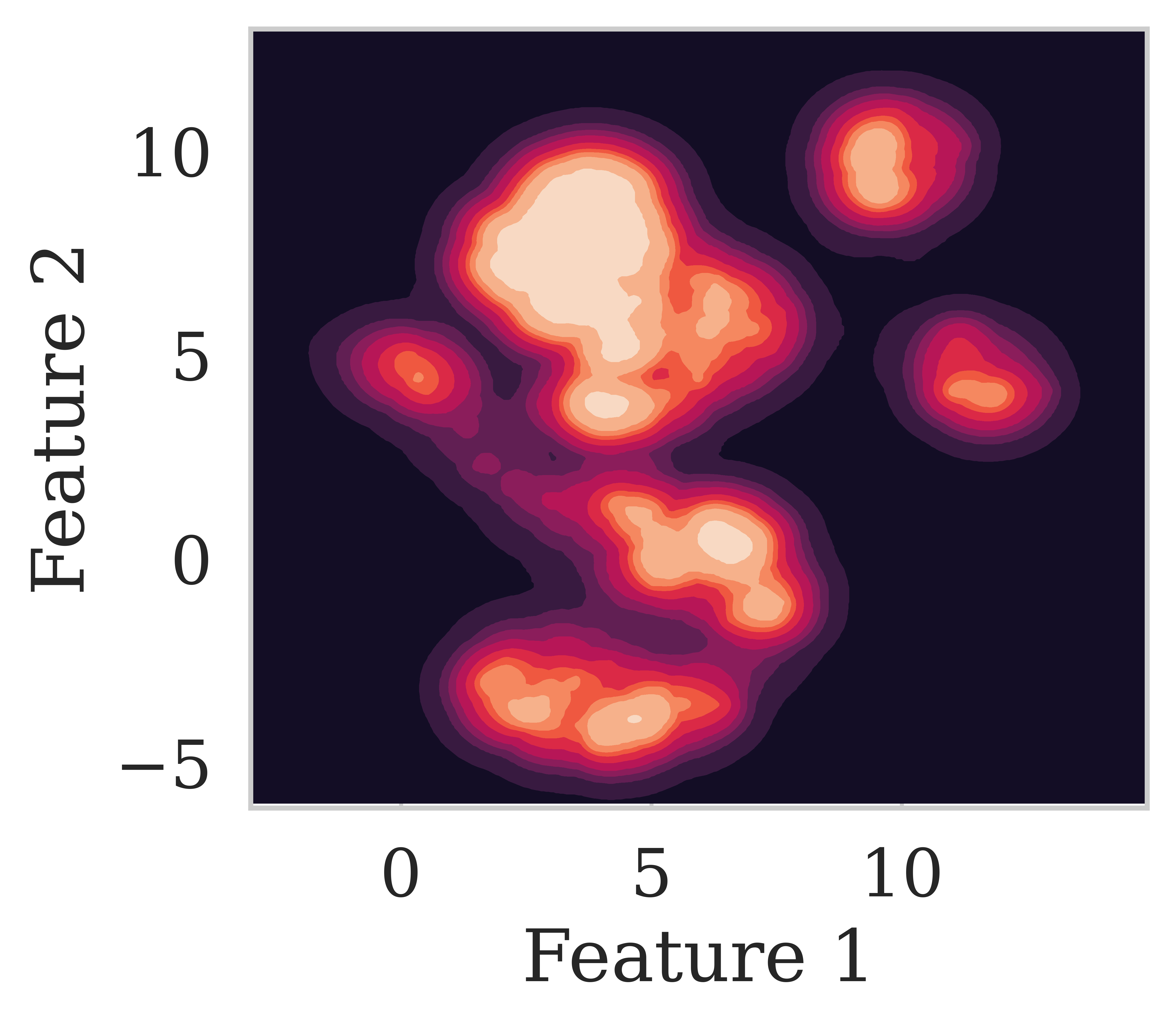
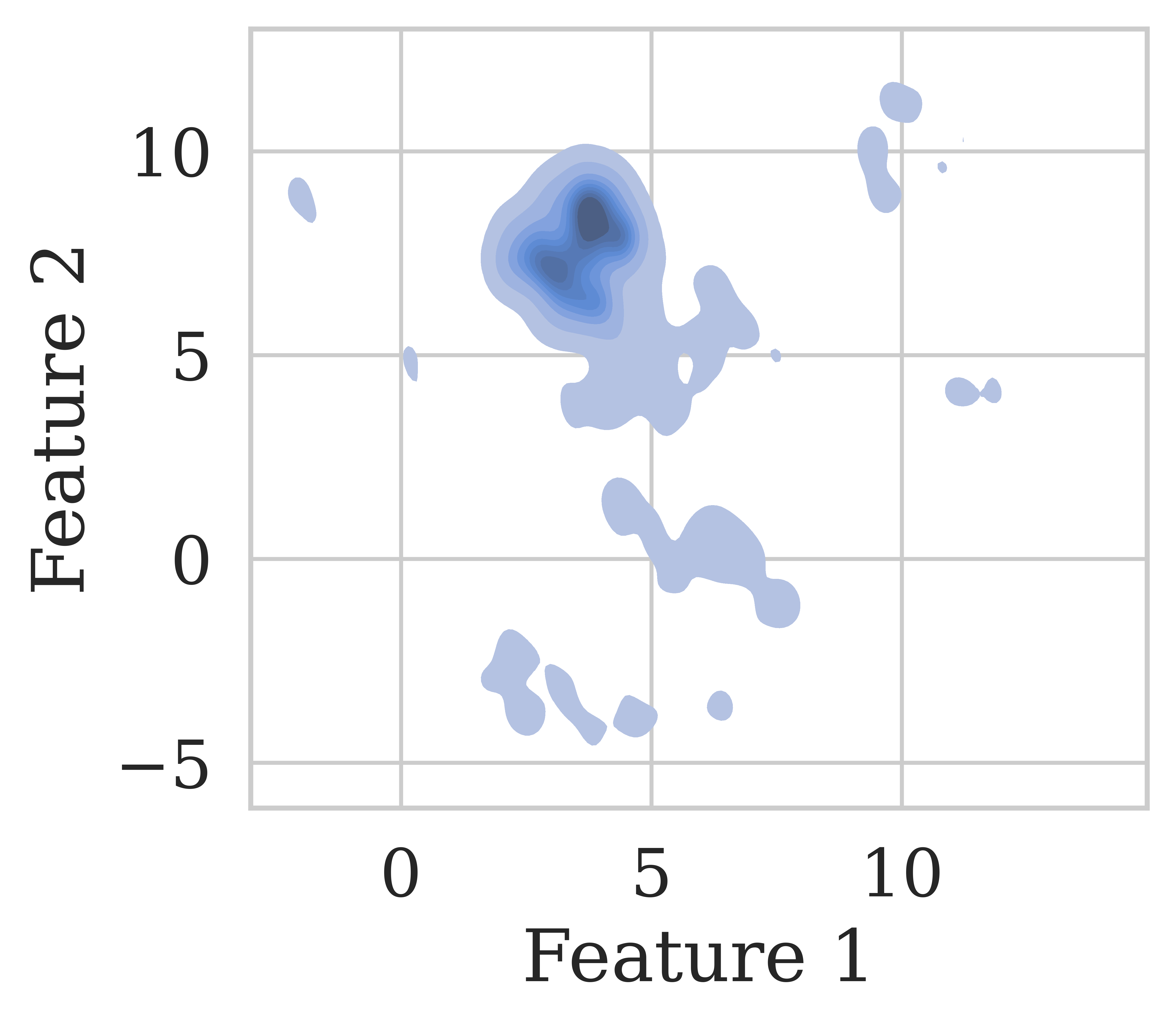
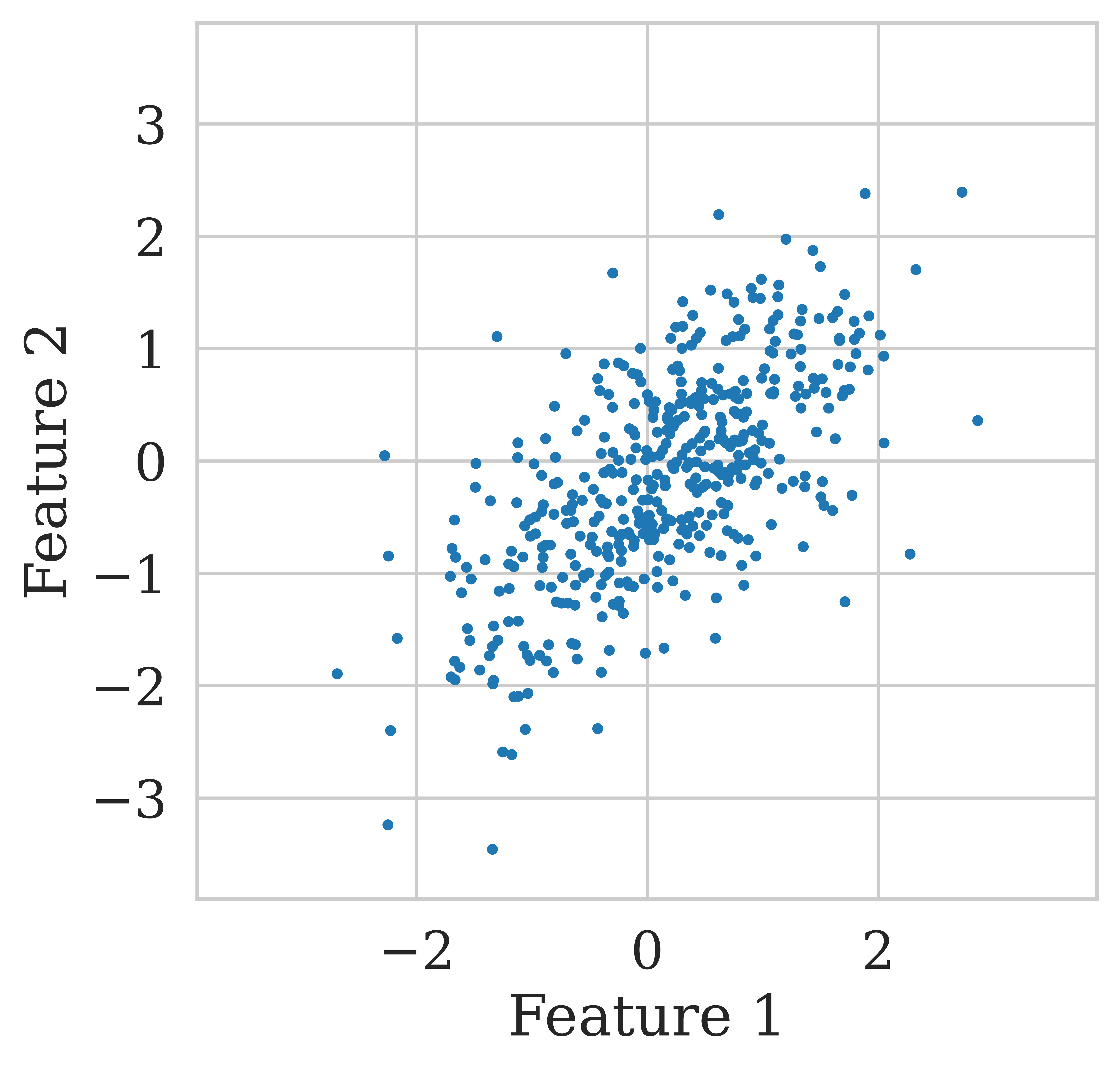
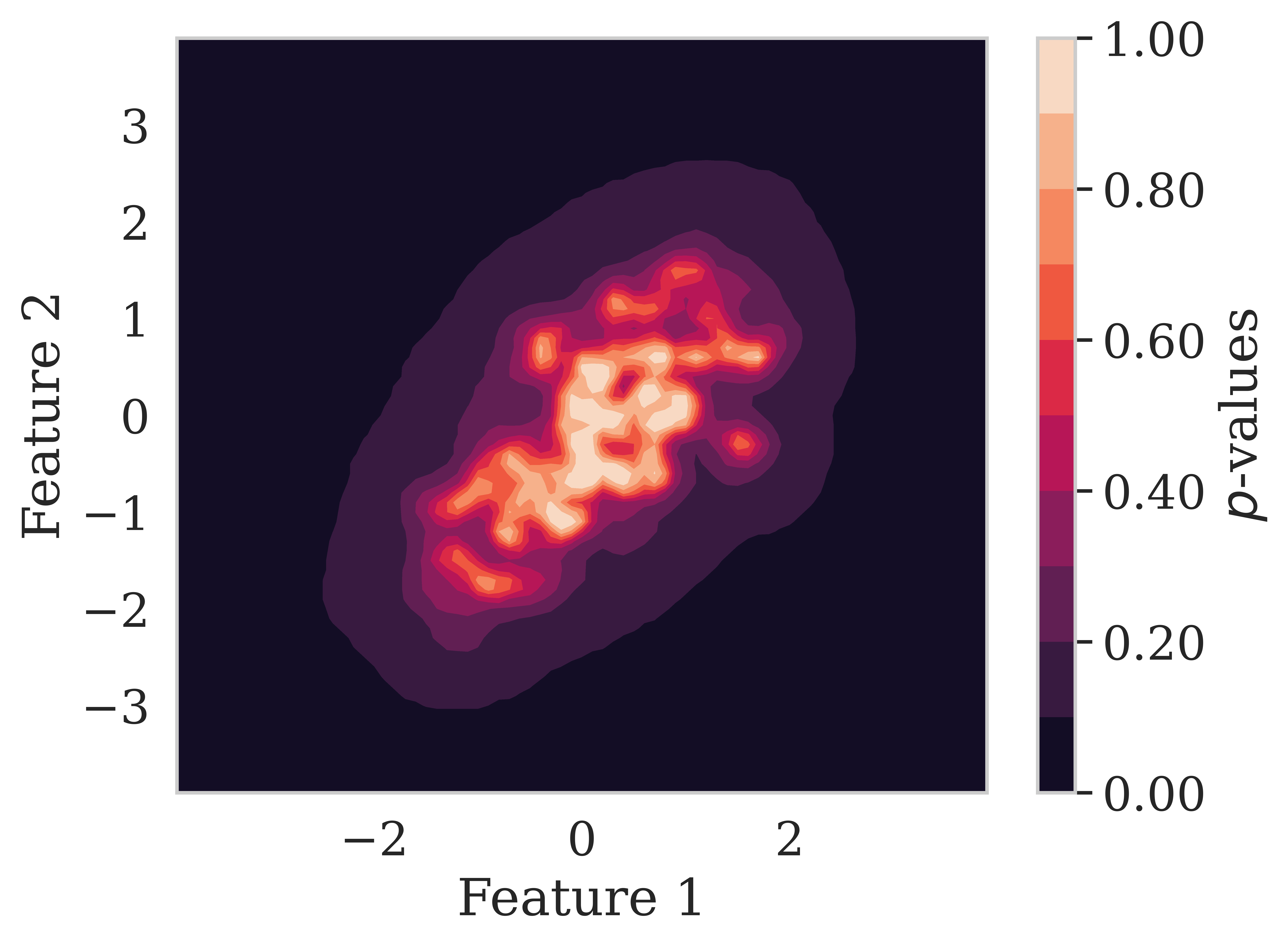
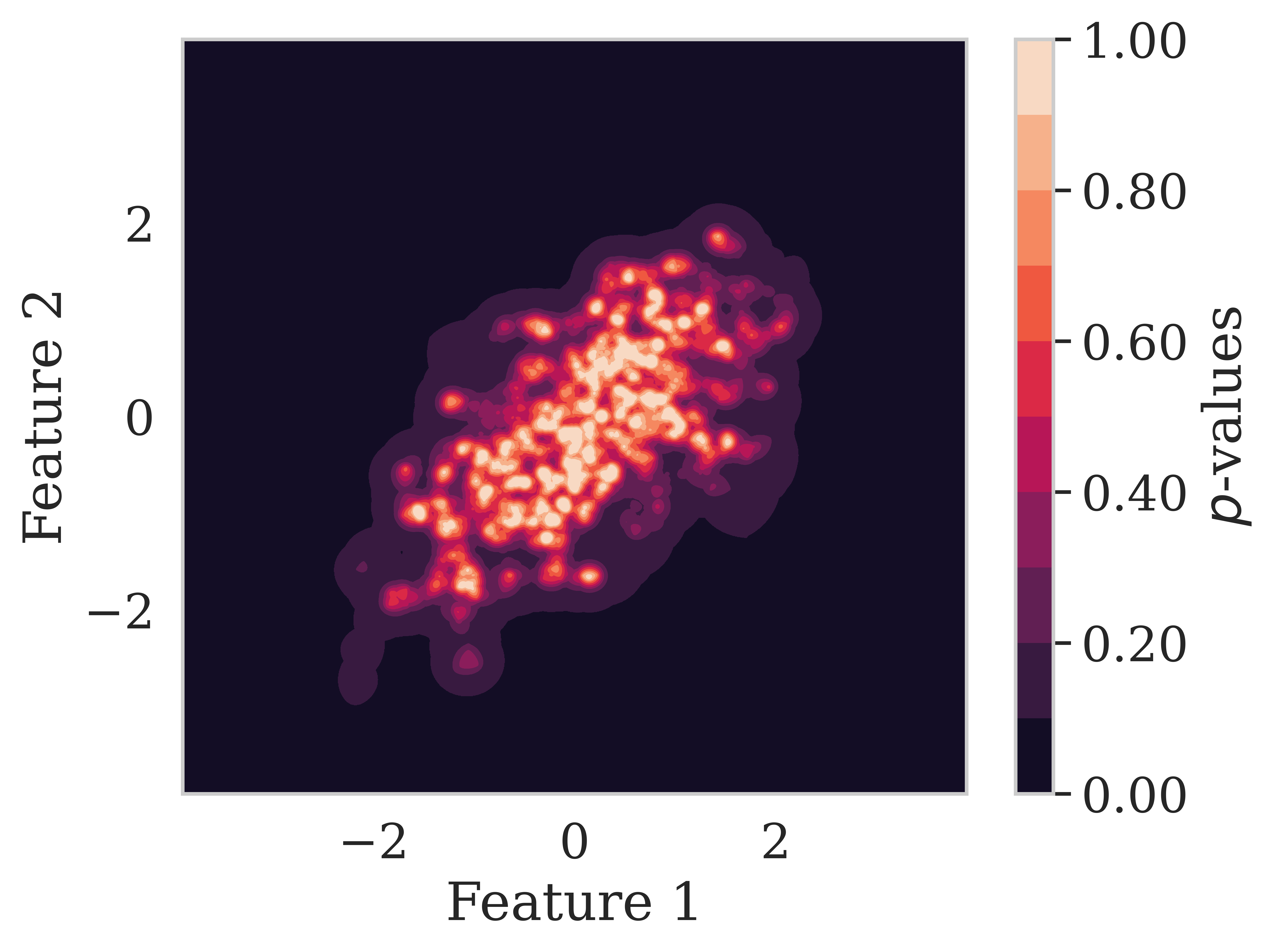
To address this challenge, we have designed a unique confident data synthesis algorithm based on a novel extension of the Conformal Prediction framework [6]. Inspired by Cherubin et al.’s innovative conformal clustering paper [7], we rely on the confidence of feature space regions to guide our data generation. Figure 1 illustrates the effect of our confidence estimation approach on the feature space compared to traditional density estimation. By limiting synthesis to the high-confidence regions, we statistically guarantee the generated data’s quality to a user-specified level. Section 1.1 details our contributions in more depth and describes the article’s structure.

(a) Original samples.

(b) Confidence regions.

(c) Density estimation.

Figure 1: Visualisation of two techniques to identify feature space regions from which data is synthesised (Figures 1(b) and 1(c)). Compared to traditional density estimation of the samples, our proposed conformal algorithm determines statistically guaranteed high-confidence regions based on a user-selected confidence threshold. The larger the threshold is, the narrower the confidence regions are, and the higher the synthesised samples’ quality is guaranteed to be.

1.1 Contributions

In this article, we propose conformalised data synthesis to reliably improve Deep Learning prediction performance on small and imbalanced datasets. Our algorithm’s statistical quality guarantees stem from uncertainty quantification founded on hypothesis testing. To the best of our knowledge, this is the first extension of the foundational Conformal Prediction confidence framework to data generation.

Inspired by the innovative conformal clustering work presented in [7], our algorithm relies on the confidence of feature space regions to reliably synthesise new, high-quality data points. Our three key contributions are:

• We incorporate ground-truth labels, making the confidence modelling process supervised,

• We identify label-conditional confidence regions in the feature space,

• And, most decisively, the confidence regions are an intermediate stage from which we synthesise new data points.

In the following sections, we will discuss the context and motivation of our data synthesis solution (Section 2); Present the design, inspiration, and theoretical foundation of our algorithm (Sections 3 and 4); And systematically evaluate the empirical advantages of our proposal on carefully selected real-world datasets of varying difficulty (Section 5).

2 Related work in data synthesis

The core concept of data synthesis is to generate previously unseen data points from an existing dataset automatically. The most popular use cases are to fully replace a dataset with synthetic samples (e.g., to address privacy concerns) [8, 9, 10], and to improve model inference with synthetic samples [11, 12, 13]. The latter is achieved by extending the training set with new samples in keeping with the original data to support model learning.

In more detail, a successfully trained classification model $h_{\theta}$ will have learned a close distribution estimation of the classes $\mathbf{Y}$ in the feature space $\mathbf{X}$, P$(Y|X)$ [14]. In other words, it will map latent variable relationships, and therefore certain feature space regions, to a particular class $y\in\mathbf{Y}$:

$$h_{\theta}(\mathbf{X})\approx\mathbf{Y}.$$ (1)

The more densely a class $y$ is represented in a region during training, the more it will be reinforced in the model’s feature space representation. However, if there are too few training samples, the model is underfit and will have learned a skewed representation of the dataset [15]. Unfortunately, collecting more data to increase the sample size is difficult in many real-world situations. Prohibitors include the high cost of data collection, low data availability, and the lack of expertise for ground-truth labelling [16].

Generative Adversarial Networks (GANs) are the most popular and ubiquitous synthesis technique used to address this concern. Introduced in [17], GANs encapsulate a zero-sum game between two models. The generator attempts to fool the discriminator with new samples synthesised from random noise. Simultaneously, the discriminator attempts to distinguish between original and generated samples. Over many training iterations, the generator’s output becomes more and more realistic [18]. However, the final synthesised output is fundamentally difficult to evaluate because there is no inherent quality metric for the GAN’s distributional fit [19, 20, 21]. We must rely on purely qualitative metrics and empirical results to estimate the samples’ quality, which may be problematic for high-risk domains such as healthcare, finance, and security [22].

Nonetheless, multiple approaches have been developed that show improved performance with empirical measures of confidence. For example, [23] interpreted the probabilistic output of the GAN’s generator and discriminator as a confidence measure. Based on this information, the synthetic samples were filtered for high scores, and empirical results for facial emotion recognition showed minor improvements. In a similar vein, [24] developed a difficulty-aware attention mechanism based on the model’s confidence for medical image segmentation. Their aim was to improve overall performance by reducing the training weights of easy samples based on a ‘confidence’ Convolutional Neural Network (CNN). The authors estimated the trustworthiness of image segments with the CNN’s confidence maps and thereby took local confidence into account. In contrast, [25] developed a sophisticated confidence model to generate pseudo-healthy images of skin lesions. Using a GAN, the authors generated subject-specific healthy images paired with a pathological sample to support classification performance. As part of the framework, they included a confidence check such that only segments with a confidence greater than a pre-defined threshold were considered for prediction.

While each of these examples improved prediction performance on specific datasets and tasks, there were no quality guarantees since the confidence measures were empirically derived from probabilistic neural network outputs. In contrast, theoretically supported confidence frameworks such as Conformal Prediction have an enormous potential to increase trust in synthesised data. However, to the best of our knowledge, Conformal Prediction has not previously been utilised for data synthesis. Apart from conformal clustering (discussed in Section 3.3), the closest related work is presented in [26]. The authors proposed the conformal framework for semi-supervised learning. In particular, Inductive Conformal Prediction was used to measure the quality of augmented samples. As a first step, the highest-confidence original samples were pre-filtered for augmentation. After augmentation, the highest-credibility adjusted samples were retained to extend the training dataset. The proposal was tested on a small dataset for herbal medicine classification, and the resulting prediction performance improved on traditional augmentation techniques. The downside was the high computational efficiency of the approach, which was further improved in [27].

As the foundation of our confident synthesis proposal, Section 3 further discusses the Conformal Prediction confidence framework in more depth.

3 Conformal Prediction background

How confident are we that a model’s prediction is correct? This is the core question uncertainty quantification techniques such as Conformal Prediction attempt to answer. To contextualise our conformal synthesis proposal (Section 4), we introduce the conformal framework (Section 3.1) and present relevant variants (Section 3.2).

3.1 The conformal framework

Conformal Prediction is a foundational confidence framework that measures the uncertainty of individual model predictions. Based on hypothesis testing, the confidence measures are statistically supported to a user-specified significance level. Under minimal exchangeability assumptions, this validity property guarantees that prediction mistakes are made up to a maximum error rate $\epsilon$ [28].

Conformal Prediction acts as a wrapper to any underlying point prediction model, making it a highly versatile confidence solution [29]. To achieve the validity property, the model’s point predictions are transformed into a prediction set $\Gamma$ including all plausible labels $y\in\mathbf{Y}$. Label inclusion is driven by the significance-level $\epsilon$, making the prediction sets $\epsilon$-dependent [30]. An error is defined as a prediction set missing a sample’s true label $y^{*}$. Due to the hypothesis testing background, the probability of a mistake being made on each sample $i$ is capped at $\epsilon$, subject to statistical fluctuations (Equation 2). By the law of large numbers, the overall probability of an error occurring approaches $\epsilon$ with increasing predictions, while the individual error probability is unchanged [31]:

$$P\left(y_{i}^{*}\notin\Gamma_{i}^{\epsilon}\right)\leq\epsilon,$$ (2)

$$\lim_{i\to\infty}\text{ avg }P\left(y_{i}^{*}\notin\Gamma_{i}^{\epsilon}\right)\approx\epsilon.$$ (3)

This strong validity guarantee is achieved through a careful construction of the prediction sets $\Gamma^{\epsilon}$. Given the original training set $Z_{train}=\Set{i=1,\ldots,n}{\left(x_{i},\text{ }y_{i}^{*}\right)}$ with samples $x\in\mathbf{X}$ and true labels $y^{*}\in\mathbf{Y}$, a test sample $x_{n+1}$’s plausibility is evaluated through extension with each possible label $y\in\mathbf{Y}$ [32]. To measure the likelihood of the postulated label given the original data, a non-conformity measure $A$ evaluates a test extension’s ‘strangeness’ with an underlying point prediction model trained on the original data:

$$\alpha^{y}=A\left(x,\text{ }y\right),\qquad\forall\quad y\in\mathbf{Y}.$$ (4)

An example of a straightforward non-conformity measure is based on the Nearest Neighbour scheme. The non-conformity score $\alpha$ measures an extended sample’s similarity to the training data by taking the sum of its $k$ nearest neighbours of the same class $y$. The larger $\alpha$ is, the further away the test sample $x$ is from a class $y$, and the less likely it is that $y$ is a plausible label [33]:

$$A(x,y)=\sum\min_{k}\text{dist}\left(\Set{i=1,\ldots,n}{y_{i}=y}\right).$$ (5)

Given the a test sample’s non-conformity scores $\alpha_{n+1}^{y}$, we may calculate the probability of each label $y$ being the true label $y_{n+1}^{*}$ via $p$-values [34]. Note that through the hypothesis testing background, all true $p$-values $p^{y^{*}}$ are automatically guaranteed to be uniformly distributed [35]:

$$p_{n+1}^{y}=\frac{\#\Set{i=1,\ldots,n,n+1}{\alpha^{y^{*}}_{i}\leq\alpha_{n+1}^{y}}}{\#\Set{i=1,\ldots,n,n+1}{i}},$$ (6)

$$p^{y^{*}}\in\mathcal{U}_{[0,1]}.$$ (7)

Finally, the prediction sets $\Gamma^{\epsilon}$ are constructed by including all labels $y$ whose confidence levels exceed the significance level $\epsilon$:

$$\Gamma^{\epsilon}=\Set{y\in\mathbf{Y}}{p^{y}>\epsilon}.$$ (8)

The larger $\epsilon$ is, the narrower the prediction set becomes, and the more likely it is that a sample’s true label $y^{*}$ is not included. Therefore, the trade-off between low error rates and precise prediction sets must be carefully balanced. The optimal classification prediction set includes exactly one label [36]. Interested readers are referred to [37] for conformal regression prediction.

3.2 Conformal Prediction variants

Though Conformal Prediction has numerous advantages, the original framework presented in Section 3.1 also comes with challenges. Consequently, variants have been proposed in the literature to counteract the drawbacks. Here, we focus on the most relevant variants to this work: Inductive Conformal Prediction and Mondrian Inductive Conformal Prediction.

As the name suggests, Inductive Conformal Prediction (ICP) adjusts the conformal learning scheme from the original transductive approach to an inductive version [38]. Without adjustment, Conformal Prediction is an online framework that requires retraining the models for every new test sample. By setting aside a dedicated, static collection of training samples, the inductive variant requires only one training iteration. Therefore, to prepare for ICP, we split the original training set $Z_{train}=\Set{i=1,...,n}{\left(x_{i},\text{ }y^{*}_{i}\right)}$ into the training proper and calibration sets $Z_{prop}=\Set{i=1,...,m}{\left(x_{i},\text{ }y^{*}_{i}\right)}$ and $Z_{calib}=\Set{i=m+1,...,n}{\left(x_{i},\text{ }y^{*}_{i}\right)}$. Given these new subsets, the non-conformity measure’s underlying algorithm is trained on $Z_{prop}$ instead of $Z_{train}$. Furthermore, the $p$-values are calculated using only the calibration set’s non-conformity scores $\alpha^{y^{*}}$:

$$p^{y}_{n+1}=\frac{\#\Set{i=m+1,\ldots,n,n+1}{\alpha^{y^{*}}_{i}\leq\alpha^{y}_{n+1}}}{\#\Set{i=m+1,\ldots,n,n+1}}.$$ (9)

This clear separation of the original data significantly reduces the algorithm’s computational complexity while maintaining guaranteed validity [39].

Building on ICP, the Mondrian Inductive Conformal Prediction (MICP) variant extends the validity property to conditional validity [40]. Without this adjustment, Conformal Prediction’s guarantees are valid over all predictions, but not necessarily per class. For example, ‘difficult’ samples part of a minority class may average higher error rates than ‘easier’ samples [41]. MICP circumvents this limitation by redefining the $p$-value equation as label-conditional [42]:

$$p^{y}_{n+1}=\frac{\#\Set{i=m+1,\ldots,n,n+1}{y^{*}_{i}=y,\text{ }\alpha^{y^{*}}_{i}\leq\alpha^{y}_{n+1}}}{\#\Set{i=m+1,\ldots,n,n+1}{y^{*}_{i}=y}},$$ (10)

$$P\left(y^{*}\notin\Gamma^{\epsilon}\mid y^{*}=y\right)\approx\epsilon,\qquad\forall\quad y\in\mathbf{Y}.$$ (11)

So far, Conformal Prediction was presented in the context of prediction tasks. Section 3.3 discusses an extension to clustering that inspired our proposed algorithm.

3.3 Conformal feature space confidence

Conformal Prediction was originally developed to measure confidence and provide performance guarantees for prediction tasks. However, the framework has since been extended to a variety of application domains, and the one most relevant to this article is unsupervised clustering.

Introduced in [7], conformal clustering is founded on measuring the conformal confidence of each point in a feature space. A grid of points represented the feature space with equal spacing to make the task discrete. By treating each grid point as a test sample, Cherubin et al. measured their unsupervised similarity to the observed training data with conformal $p$-values (Section 3.1). All grid points with $p>\epsilon$ were considered part of the clusters, where $\epsilon$ was a user-specified threshold between 0 and 1. The clusters themselves were defined via the neighbouring rule: two grid points were part of the same cluster if they were neighbours. Therefore, in addition to setting the confidence threshold, $\epsilon$ may be considered as a regularisation factor of the clusters’ connectedness. The smaller $\epsilon$ was, the more connected the high-confidence grid points were, and the fewer distinct clusters were formed.

Building on this work, Nouretdinov et al. further underpinned the understanding of conformal clustering in [43]. The authors extended the approach to develop multi-level conformal clustering, introducing a dendrogram construction similar to traditional hierarchical clustering methods. Additionally, a new technique for identifying out-of-distribution anomalies was established by testing whether new samples fell within a conformal cluster.

For the purpose of our proposed synthesis algorithm, the conformal clustering concept of measuring feature space confidence is particularly interesting. For a successful synthesis, we would expect the new samples to fall within the original data distribution. By limiting synthesis to high-confidence feature space regions, anomalies should be minimised to a user-specified level. With this inspiration, Section 4 introduces our proposed confident data synthesis algorithm.

4 Conformalised data synthesis

In this section, we propose a unique data synthesis algorithm that introduces statistical confidence to the data generation process. The basis of our confidence measure is the foundational Conformal Prediction framework, traditionally used for prediction and distribution testing tasks (Section 3). Our work presents a novel extension of the conformal technique to data generation, a previously unexplored domain. After examining our proposal’s implications for the synthesised data (Section 4.1), we comprehensively discuss our algorithm’s design, theoretical guarantees, and practical characteristics (Section 4.2).

4.1 Implications for data generation

Inspired by the innovative conformal clustering work presented in [7] (Section 3.3), our novel conformal data synthesis algorithm relies on the confidence of feature space regions to generate high-quality data points reliably. By limiting synthesis to the high-confidence regions, we statistically guarantee the generated data’s quality to a user-specified significance level $\epsilon$. Consequently, unlike traditional synthetic data generation techniques (Section 2), our conformal synthesis algorithm models a selective distribution of the original dataset.

The confidence regions are identified by comparing the relative differences in label-conditional non-conformity scores. Therefore, the definition of the non-conformity function significantly impacts how the original data’s distribution is modelled. This flexibility is an inherent advantage of the Conformal Prediction framework and allows adjustments to be made that best suit the dataset and classification task for improved performance. For example, we could prioritise maintaining intra-class relationships by incorporating distances between classes or reducing noise by lowering outliers’ importance.

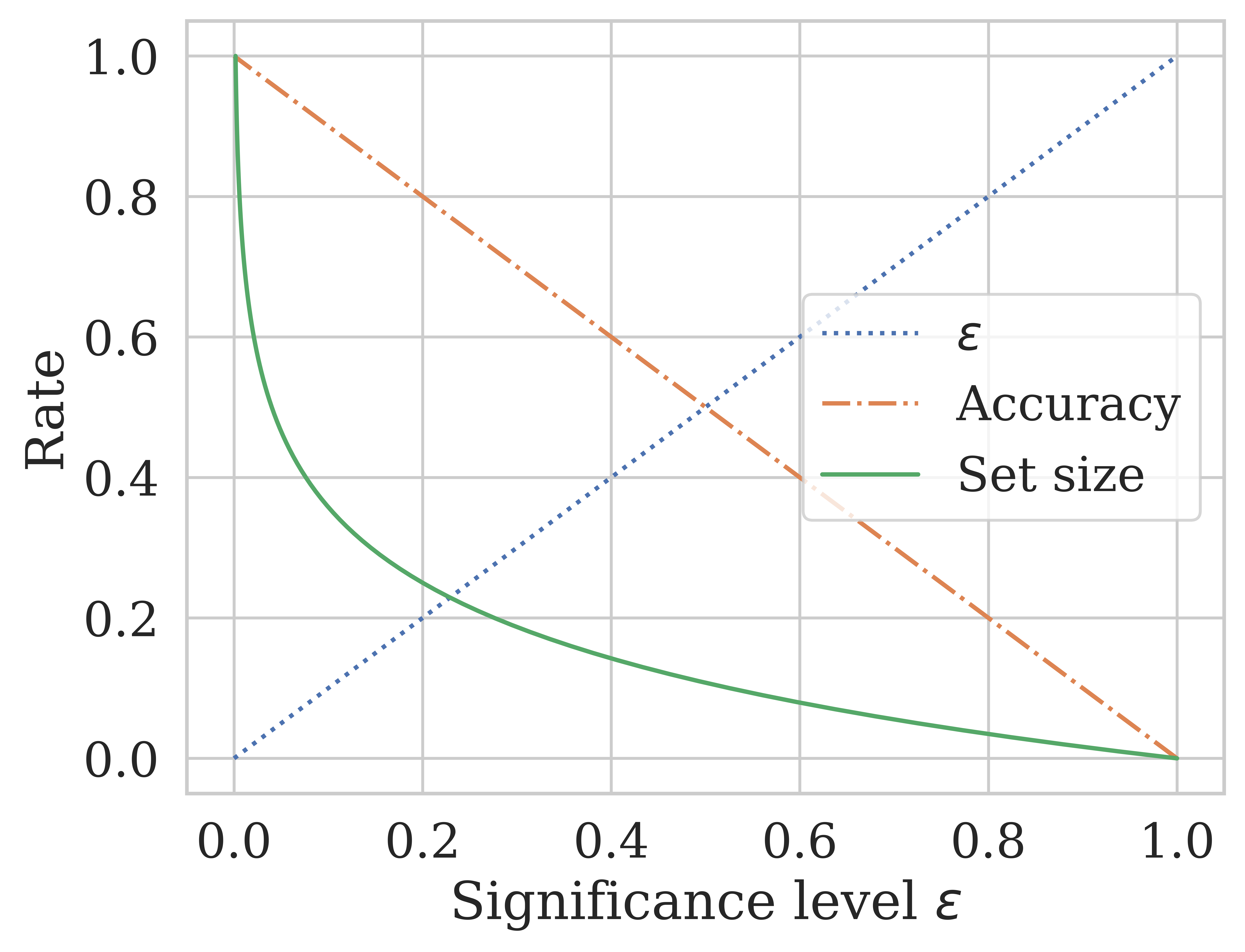
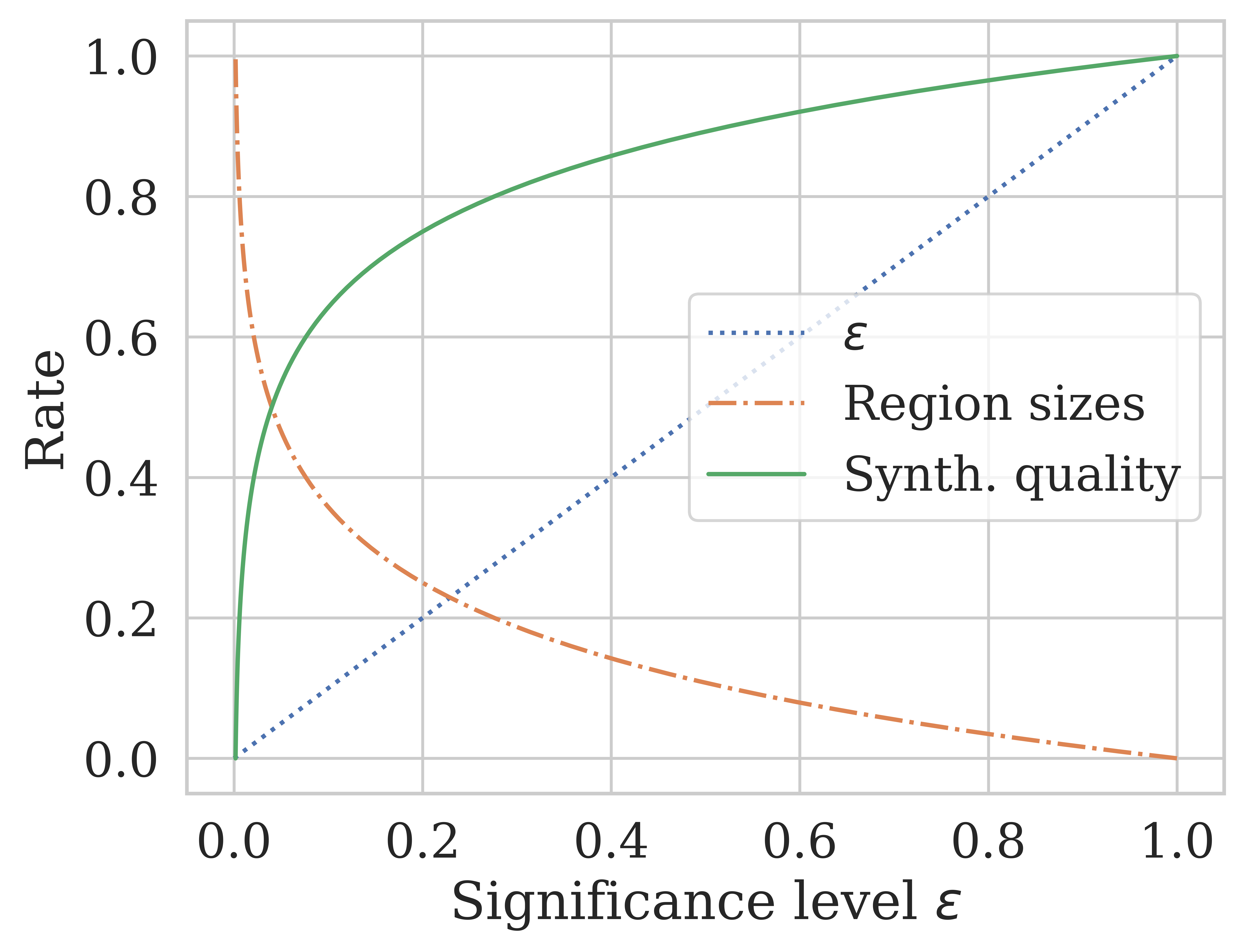
Driven by the data generation domain, we redefine what we understand as an error. For a traditional Conformal Prediction task, an error is defined as the absence of a sample’s true label from its prediction set. The significance level $\epsilon$ regulates the trade-off between our desire for narrow prediction sets and ensuring a sample’s true label is still included. However, for confident data synthesis, our priority is to identify and reinforce the most representative feature space regions for Deep Learning training. Consequently, an error is defined as the inclusion of non-representative areas in the high-confidence regions. Effectively, the significance level’s desirability is inverted. The larger $\epsilon$ is, the more tightly controlled the confidence regions are, and the more we exclude low-confidence synthetic data. In other words, we re-interpret $\epsilon$ as the generated data’s quality or closeness to the original data. Figure 2 visualises $\epsilon$’s effect.

(a) Conformal Prediction classification.

(b) Conformal synthesis.

Figure 2: Visualisation of the $\epsilon$ trade-off between conformal accuracy and precision. Traditional conformal classification prefers smaller $\epsilon$ to optimise prediction sets. In contrast, conformal synthesis relies on large $\epsilon$ to more carefully control confidence region sizes and, consequently, the synthesised samples’ quality.

With this understanding of our proposal’s implications, Section 4.2 details the algorithm’s steps and characteristics.

4.2 Proposed algorithm

Algorithm 1 illustrates the logical flow of our proposed algorithm. Given a feature space $\mathbf{X}\in\mathcal{R}^{d}$, we construct a grid point representation $\mathbf{G}^{\gamma}\in\mathcal{R}^{d}$ of $\mathbf{X}$ with grid step $\gamma$ such that all observed samples $x\in\mathbf{X}$ fall within its boundaries. $\mathbf{X}_{grid}$ represents the collection of all grid points in $\mathbf{G}^{\gamma}$ (3). To prepare for Inductive Conformal Prediction, the training data $Z_{train}=\left(\left(x_{1},y_{1}\right),\ldots,\left(x_{n},y_{n}\right)\right)$ with $x\in\mathbf{X}$ and $y\in\mathbf{Y}$ is split into the training proper and calibration subsets $Z_{prop}=\left(z_{1},\ldots,z_{m}\right)$ and $Z_{calib}=\left(z_{m+1},\ldots,z_{n}\right)$. Then, we calculate the non-conformity scores $\alpha^{y}_{calib}$ of each point in the calibration set (4 and 5). We rely on a neighbour-based non-conformity measure $A$, defined in Equation 5 in Section 3.1.

Algorithm 1 Logical flow of the proposed conformal synthesis algorithm. Section 3 defines the non-conformity measure $A$ (Equation 5), the $p$-value formula (Equation 10), and how the training set $Z_{train}$ is split (Section 3.2).

1:Non-conformity measure $A$, grid step $\gamma$, significance level $\epsilon$, training set $Z_{train}=\left(x\in\mathbf{X},\text{ }y\in\mathbf{Y}\right)$

2:$\textbf{X}\in\mathcal{R}^{d},\text{ }\textbf{Y}\in\mathcal{N},\text{ }0\leq\epsilon\leq 1$

3:$\mathbf{X}_{grid}\Leftarrow\mathbf{G}^{\gamma}\in\mathbf{X}$

4:$Z_{prop},Z_{calib}\Leftarrow\text{split}\left(Z_{train}\right)$

5:$\alpha^{y}_{calib}\Leftarrow A\left(Z_{calib}\right)$

6:for $y\in\textbf{Y}$ do

7:     $\alpha^{y}_{grid}\Leftarrow A\left(\left(\mathbf{X}_{grid},\text{ }y\right)\right)$

8:     $p^{y}_{grid}\Leftarrow\text{calculate\_p\_values}\left(\alpha^{y}_{calib},\text{ }\alpha^{y}_{grid}\right)$

9:     $\mathbf{R}_{y}^{\epsilon}\Leftarrow\Set{x_{grid}\in\mathbf{X}_{grid}}{p^{y}_{grid}>\epsilon}$

10:end for

11:$Z_{syn}\Leftarrow\Set{\left(x_{grid}\in\mathbf{X}_{grid},\text{ }y\in\textbf{Y}\right)}{x_{grid}\in\mathbf{R}_{y}^{\epsilon}}$

7, 8 and 9 contain the core of our confident data synthesis logic. To synthesise high-quality data points, we must first evaluate the confidence of each point in the feature space, represented by $\mathbf{X}_{grid}$. In Conformal Prediction terminology, we are treating the grid points as test samples, extending them with each possible class label $y\in\mathbf{Y}$. Given the label-conditional non-conformity scores $\alpha^{y}_{grid}$, we calculate $p^{y}_{grid}$ following the Mondrian Inductive Conformal scheme (Equation 10 in Section 3.2). The $p$-values represent each grid point’s likelihood of being assigned class $y$, assuming it is indeed representative of class $y$. In other words, these $p$-values establish our confidence in a region’s representation of a particular class. The threshold for the label-conditional confidence regions $\mathbf{R}_{y}^{\epsilon}$ is the user-selected significance-level $\epsilon$. With this information, all grid points falling into the high-confidence regions $\mathbf{R}_{y}^{\epsilon}$ are sampled as synthetic data points $Z_{syn}$ with their matching class label $y$ (11). Note that synthetic data points $x_{syn}$ in overlapping high-confidence regions are extended and included in $Z_{syn}$ multiple times, once for each relevant class (e.g., when classes overlap in the feature space).

Derived from the validity property of Conformal Prediction (Theorem 1), we can make quality guarantees about our synthetic data’s distributional fit of the original dataset (Lemma 2 and Theorem 3).

Theorem 1.

Traditional Conformal Prediction automatically satisfies the validity property of its prediction sets. The probability of a true label $y^{*}$ being excluded from the $\epsilon$-dependent prediction set $\Gamma^{\epsilon}$ is at most $\epsilon$ (interested readers are referred to [44] for the full proof):

$$\Gamma^{\epsilon}=\Set{y\in\mathbf{Y}}{p^{y}>\epsilon},$$ (12)

$$\text{P}\left(y^{*}\notin\Gamma^{\epsilon}\right)\leq\epsilon.$$ (13)

Lemma 2.

Using Equation 12, the class-conditional high-confidence regions $\mathbf{R}_{y}^{\epsilon}$ may be redefined as the set of grid points $x_{grid}$ whose prediction sets $\Gamma^{\epsilon}$ include the class $y$:

$$\mathbf{R}_{y}^{\epsilon} =\Set{x_{grid}\in\mathbf{X}_{grid}}{p^{y}_{grid}>\epsilon},$$ (14)

$$=\Set{x_{grid}\in\mathbf{X}_{grid}}{y\in\Gamma^{\epsilon}}.$$ (15)

Theorem 3.

Building on Theorem 1 and Lemma 2, feature space points that are representative of a class $x^{y^{*}}_{grid}$ will be included in the high confidence regions $\mathbf{R}_{y}^{\epsilon}$ with a guaranteed probability of up to $1-\epsilon$:

$$\text{P}\left(y^{*}\notin\Gamma^{\epsilon}\right)=\text{P}\left(x^{y^{*}}_{grid}\notin\mathbf{R}_{y}^{\epsilon}\right),$$ (16)

$$\text{P}\left(x^{y^{*}}_{grid}\notin\mathbf{R}_{y}^{\epsilon}\right)\leq\epsilon,$$ (17)

$$\text{P}\left(x^{y^{*}}_{grid}\in\mathbf{R}_{y}^{\epsilon}\right)\geq 1-\epsilon.$$ (18)

Regarding practical properties, the algorithmic complexity is strongly influenced by the Inductive Conformal Prediction variant [45]. Assuming the underlying algorithm’s training and application complexities $U_{t}$ and $U_{a}$, the number of original training samples $n$, the number of calibration samples $m$, and the number of grid points $g$, the algorithmic complexity can be described as:

$$\Theta\left(m\cdot U_{t}+\left(n-m+g\right)\cdot U_{a}\right).$$ (19)

The largest individually contributing step is evaluating the per-class confidences of each point in the grid space (7 and 8 in Algorithm 1). However, due to the inductive variant, this step is fully parallelisable both within and between classes. Furthermore, as long as the original data set is unchanged, the grid’s $p$-values may be reused to generate confidence regions for any significance level $\epsilon$. Finally, the proposed algorithm’s parameters may strongly influence the synthesised output and are investigated in depth in Section 5.2.

In summary, our proposed conformal algorithm is a unique approach to introduce statistical confidence to the data synthesis process. Motivated by previous work, we build on the Conformal Prediction framework to support our confidence measure with hypothesis testing and guarantee synthesis quality. With this background, Section 5 investigates our algorithm’s empirical results on real-world datasets.

5 Empirical results

In this section, we comprehensively evaluate our proposed algorithm’s performance on real-world data. In particular, we investigated the following research questions:

• What influence do the conformal synthesis parameters have on the synthesised data? (Section 5.2)

• To what degree does conformal synthesis improve Deep Learning performance on small and large datasets? (Section 5.3.1)

• How effective is conformal synthesis at equalising Deep Learning performance on highly imbalanced classes? (Section 5.3.2)

• Can we successfully improve the quality of a dataset with overlapping classes by extending it with synthetic data points? (Section 5.3.3)

• How accurately can we replace a real-world dataset with entirely synthetic examples? (Section 5.3.4)

5.1 Experimental setup

We carried out a rigorous empirical evaluation of the synthetic data points produced by our proposed conformal synthesis algorithm (Section 4.2). Because the expected use case is to bolster datasets with few samples for Machine Learning, we evaluated the quality of our generated data by measuring the performance of a Deep Learning model trained on it.

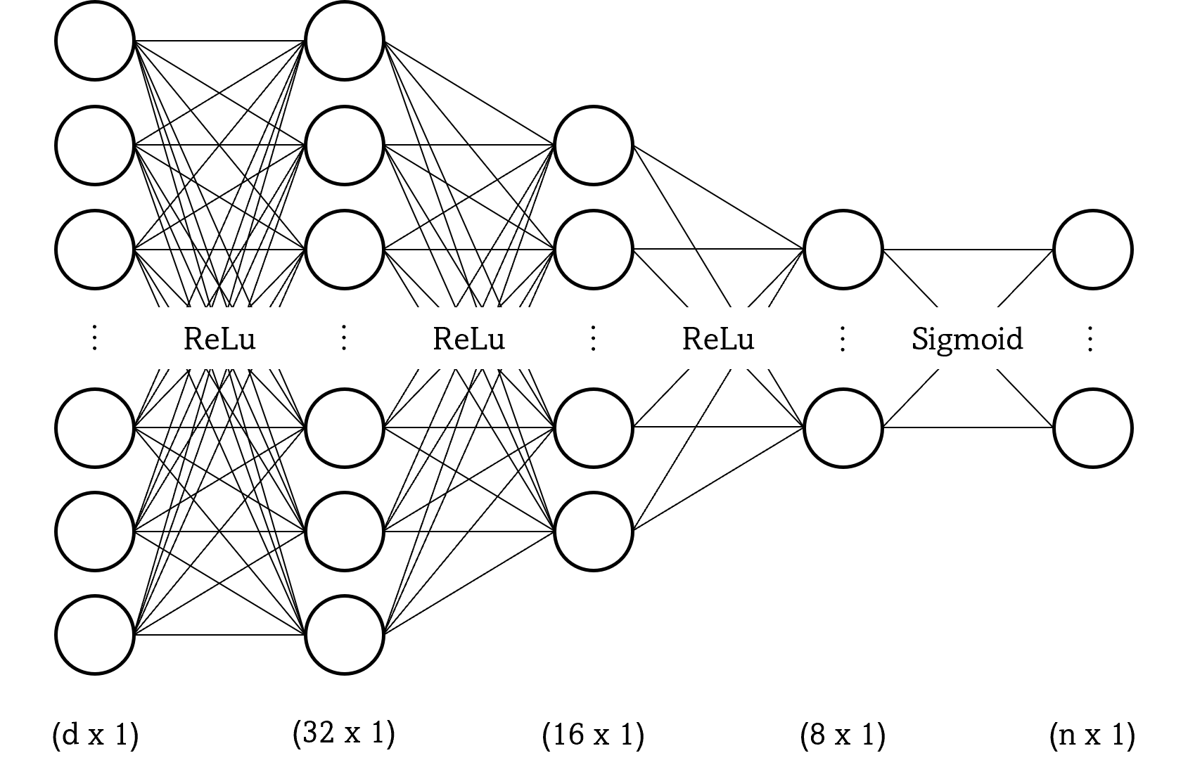
We chose a feedforward neural network with three hidden layers for the model, as shown in Figure 3. The model’s architecture and parameters were chosen for their versatility and robustness to ensure a good baseline performance on all five selected datasets. The activation functions are the popular ReLu function and the Sigmoid function for a classification output. The number of output nodes was adjusted based on the evaluated dataset’s number of classes. The model was trained for ten epochs with early stopping enabled in all trials.

Figure 3: The Deep Learning model architecture used in all trials. Design decisions were made to improve the versatility for different real-world datasets and the robustness of the results. The input layer size $d$ and output layer size $n$ are driven by the dataset’s dimensionality and number of classes.

Our primary performance metrics were the total and per-class F₁-scores. Unlike alternatives like accuracy and ROC-AUC, the F₁-score is robust against dataset imbalances. The per-class $F^{c}_{1}$ is defined as the harmonic mean of precision $P^{c}$ and recall $R^{c}$, which in turn are calculated from the true positive $TP$, the false positive $FP$, and the false negative $FN$ rates:

$$P^{c} =\frac{TP}{TP+FP},$$ (20)

$$R^{c} =\frac{TP}{TP+FN},$$ (21)

$$\text{F}^{c}_{1} =2\cdot\frac{P^{c}\cdot R^{c}}{P^{c}+R^{c}}.$$ (22)

To ensure that the results were representative regardless of variance in the model’s training, we repeated each experiment five times and reported the macro-average of all per-class scores:

$$P =\frac{\sum_{c\in C}P^{c}}{|C|},$$ (23)

$$R =\frac{\sum_{c\in C}R^{c}}{|C|},$$ (24)

$$\text{F}_{1} =\frac{\sum_{c\in C}\text{F}^{c}_{1}}{|C|}.$$ (25)

For a meaningful comparison of the Deep Learning model’s performance on the original data vs our synthesised data, each trial was evaluated on the same test set. Figure 4 illustrates in more detail how the data was split and the evaluated training data configurations.

Figure 4: The proposed conformal synthesis algorithm aims to improve the quality of the training data. To robustly evaluate our proposal’s performance, we compare a Deep Learning model’s results on the same test set when trained on the original training set Train${}_{\text{orig}}$, the set of synthetic samples Train${}_{\text{syn}}$, and their combination, the extended training set Train${}_{\text{ext}}$.

5.2 Illustrating the parameters’ influence

We employed a simple toy dataset to demonstrate the influence of our proposed data synthesis algorithm’s three parameters: the grid step $\gamma$, the significance level $\epsilon$, and the number of original training samples $n$.

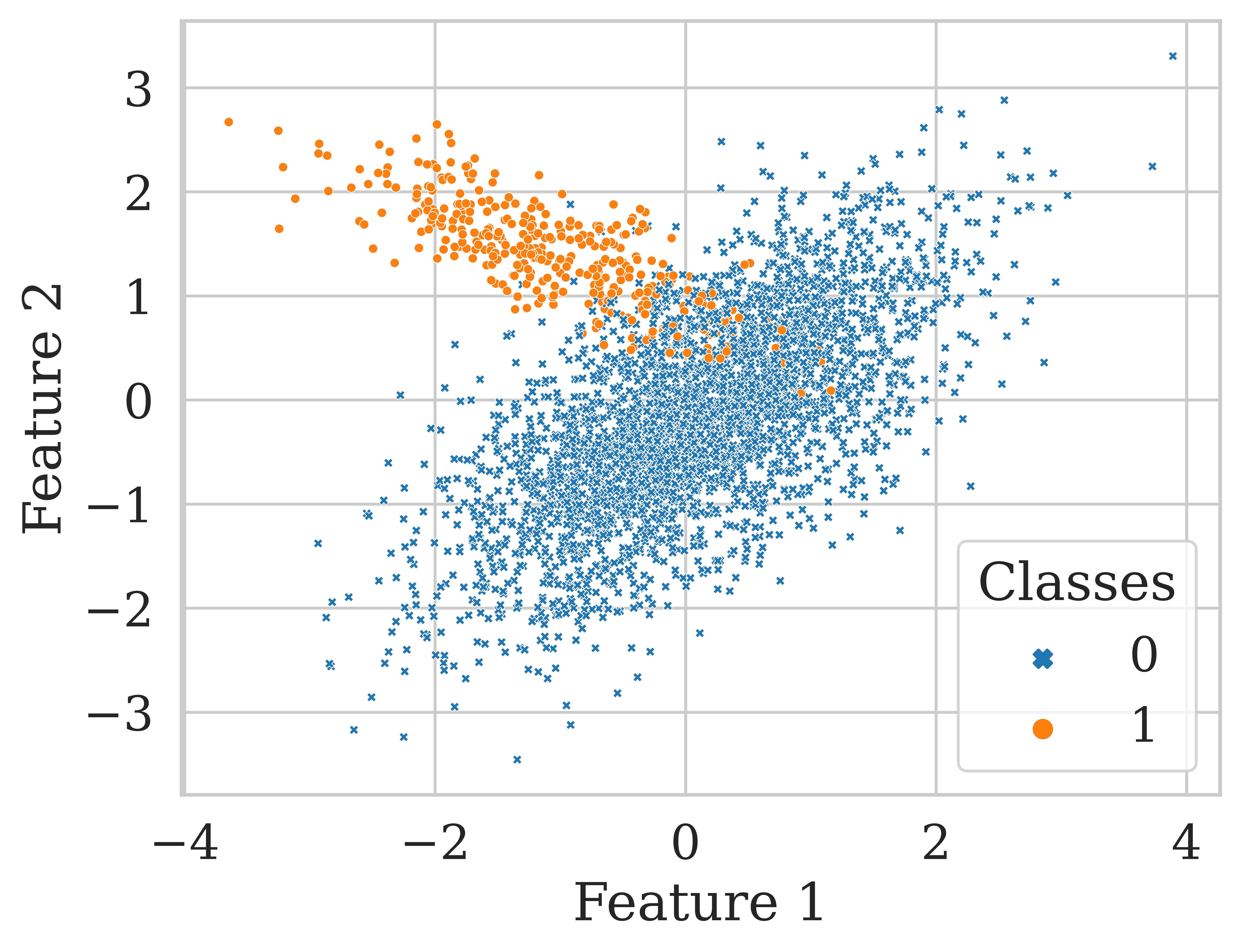
Visualised in Figure 5, the 2-dimensional classification dataset was generated with 4,000 samples and a 1:9 class imbalance. The two classes show a slight overlap in the feature space to make the classification task more challenging, but with an otherwise relatively clear class distinction. We limited the training set to 1,000 samples to simulate a small dataset, and the remaining 3,000 samples were used to robustly evaluate the Deep Learning model’s performance (architecture and training details are given in Section 5.1).

Figure 5: A straightforward 2-dimensional toy dataset used to illustrate the influence of the proposed algorithm’s parameters.

5.2.1 Grid step $\gamma$

The grid step $\gamma$ defines the resolution of our feature space, bounded by the minima and maxima of the original dataset’s features. Each grid point may be thought of as a potential synthetic sample with label-conditional $p$-values, which are tested against the significance level $\epsilon$. Therefore, the smaller $\gamma$ is, the more synthetic data points will be sampled from our high-confidence feature space regions, as shown in Figure 6. A higher density of synthetic samples is desirable because Deep Learning models tend to generalise better with larger training sets. However, the trade-off is higher required computing power, as each grid point must be evaluated per class. In areas where the classes’ high-confidence regions overlap (most likely due to non-linearly separable classes in the original dataset), both classes are assigned the same synthetic samples.

(a) $\gamma=0.1$.

(b) $\gamma=0.05$.

Figure 6: Effects of the grid step $\gamma$ on the feature space’s resolution. The points in the graphs represent the grid points that fall into the outlined high-confidence regions ($\epsilon=0.8$). A smaller $\gamma$ means that a higher density of synthetic samples may be generated from the same high-confidence regions.

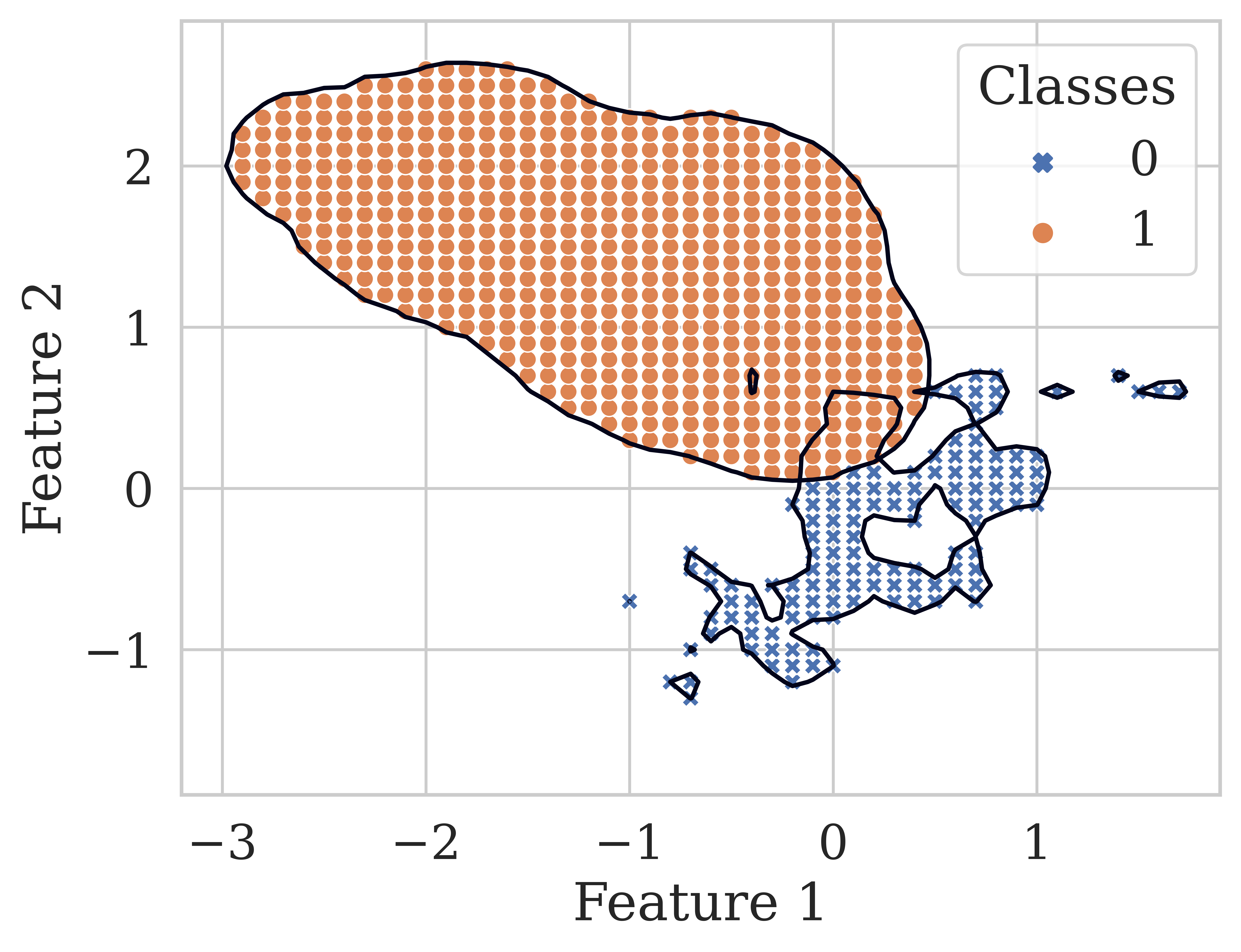
Table 1 shows these effects on our toy dataset. Varying only $\gamma$ while holding the other parameters steady, we found that the number of synthetic samples generated from the exact same high-confidence regions significantly increased with a decrease in the grid step. Consequently, the same Deep Learning model’s generalisation performance increased by 30%: from F₁ = 55% when trained on the dataset extended with $\gamma=0.1$, to F₁ = 85% when trained on the dataset extended with $\gamma=0.005$. Additionally to the improved generalisation, the reduction of the F₁-score’s standard deviation by a factor of 10 indicates that the models were trained more robustly. In particular, Recall scores were significantly increased due to the stronger representation of the minority class with an increased sample count.

Table 1: Mean Deep Learning prediction results with varying grid step $\gamma$. The grid step defines the resolution of the feature space grid. The smaller $\gamma$ is, the more synthetic samples are generated. Consequently, the model’s generalisation is significantly improved. The model was trained on the original and extended training sets ($\epsilon=0.9$, $n=100$).

	Training samples			F1-score		Precision		Recall
$\mathbf{\gamma}$	orig.	syn.	ext.	Trainorig	Trainext	Trainorig	Trainext	Trainorig	Trainext
0.1	100	387	487	0.59 (.10)	0.55 (.22)	0.71 (.20)	0.63 (.06)	0.65 (.15)	0.77 (.14)
0.05	100	1525	1625	0.59 (.10)	0.74 (.06)	0.71 (.20)	0.71 (.04)	0.65 (.15)	0.87 (.03)
0.005	100	152628	152728	0.59 (.10)	0.85 (.01)	0.71 (.20)	0.82 (.01)	0.65 (.15)	0.90 (.00)

5.2.2 Significance level $\epsilon$

Inherited from the Conformal Prediction framework, the significance level $\epsilon$ is a central parameter of our proposed algorithm. With it, a user may set the statistically guaranteed minimum confidence threshold for data synthesis. Given the $p$-values of each point in the feature space grid, we identify the per-class high-confidence regions where $p>\epsilon$.

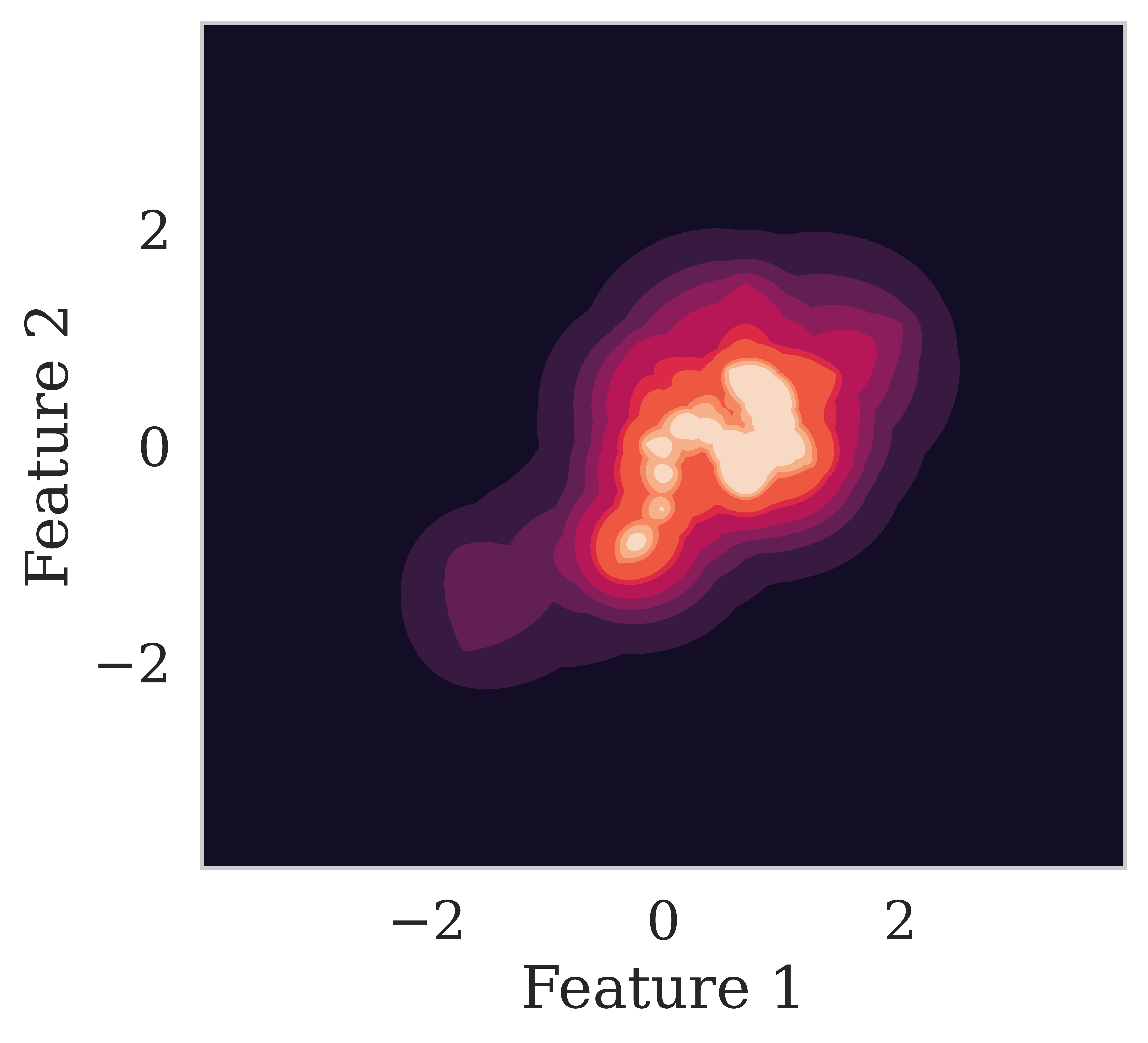
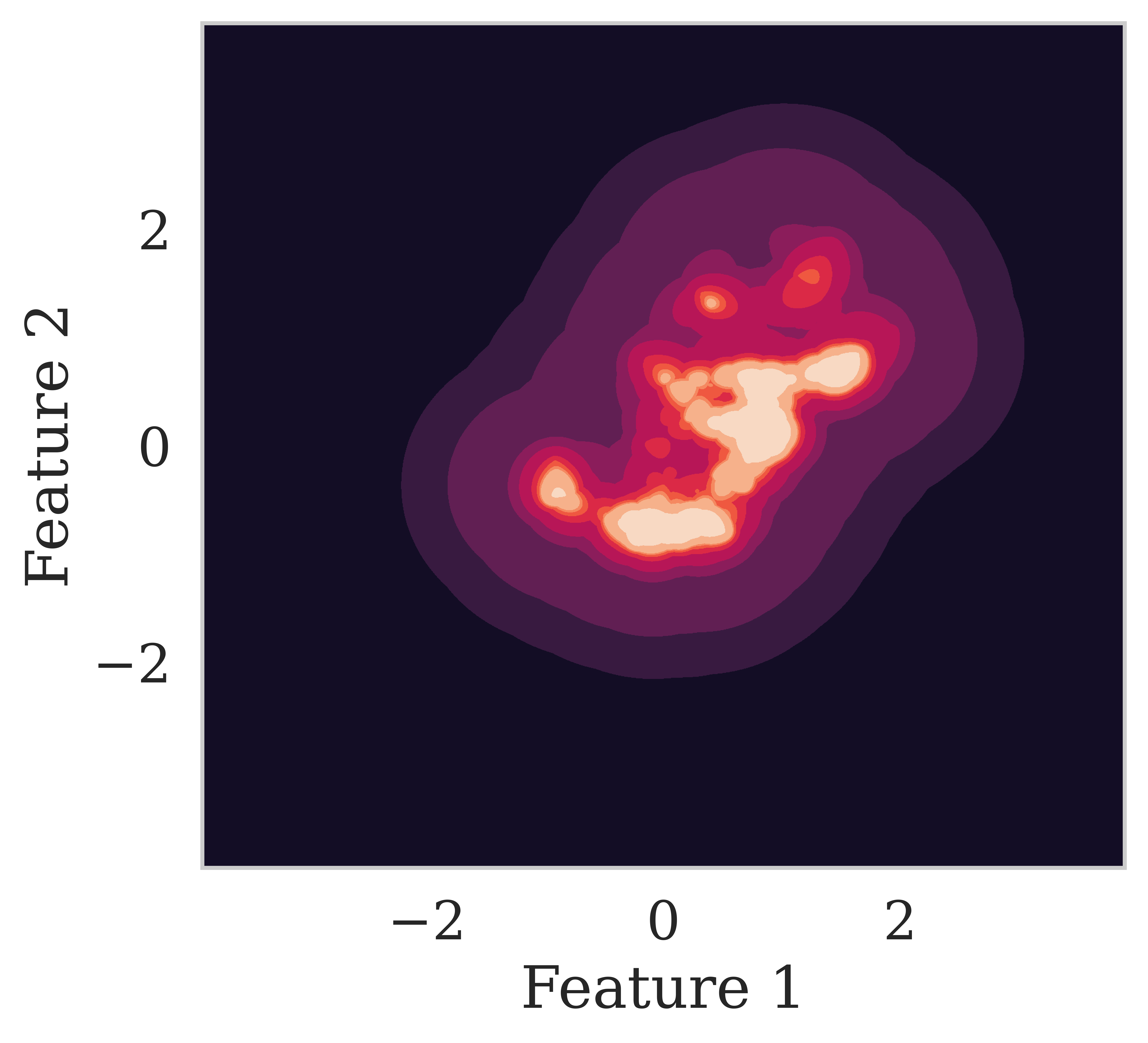
Compared to traditional Conformal Prediction, we reinterpret $\epsilon$ as the synthetic data’s closeness to the original distribution (Section 4.1). The larger $\epsilon$ is, the more carefully we control the high-confidence regions, tightening them around the existing data points. For example, we may choose a higher significance level to give less importance to outliers. Alternatively, a lower significance level for a dataset with low variance would lead to a larger number of synthetic samples without introducing as much noise. In general, larger $\epsilon$ are desirable because they limit data synthesis to the more clearly representative feature space regions, as visualised in Figure 7.

(a) Original training samples.

(b) Feature space $p$-values.

Figure 7: Effects of the significance level $\epsilon$ on the feature space’s confidence regions. The figures show class 0 of the toy dataset. Synthetic samples are generated from high-confidence regions, defined as $p>\epsilon$. The larger $\epsilon$ is, the more controlled the high-confidence regions are around the original training samples.

The effects on Deep Learning performance are illustrated in Table 2. Even though increasing the significance level shrunk the high-confidence regions (and consequently the number of generated synthetic samples) dramatically, Deep Learning performance improved significantly. This is because the quality of the synthetic samples was increased, strengthening the classes’ representations in the prediction model (from 59% on the original dataset to 88% F₁-score with $\epsilon=0.95$).

Table 2: Mean Deep Learning prediction results with varying significance level $\epsilon$. The larger $\epsilon$ was, the smaller the confidence regions were, and the fewer synthetic samples were generated. However, the quality of the synthetic samples increased in inverse proportion, significantly improving the model’s learning. Training was carried out on the original and extended training sets ($\gamma=0.005$, $n=100$).

	Training samples			F1-score		Precision		Recall
$\mathbf{\epsilon}$	orig.	syn.	ext.	Trainorig	Trainext	Trainorig	Trainext	Trainorig	Trainext
0.80	100	369584	369684	0.59 (.10)	0.68 (.01)	0.71 (.20)	0.66 (.00)	0.65 (.15)	0.86 (.01)
0.90	100	152628	152728	0.59 (.10)	0.85 (.01)	0.71 (.20)	0.82 (.01)	0.65 (.15)	0.90 (.00)
0.95	100	56746	56846	0.59 (.10)	0.88 (.01)	0.71 (.20)	0.85 (.01)	0.65 (.15)	0.90 (.00)

5.2.3 Original training sample count $n$

To synthesise new data points with our proposed algorithm, we must first identify the feature space’s high-confidence regions. The more representative the original training points are, the more precisely we can identify the most informative regions for data synthesis and the higher the quality of the synthetic points will be. In practice, we may assume that the larger the original dataset is, the more prediction performance improvement we will achieve. This relationship is illustrated in Figure 8 and Table 3. With an increase in the number of original training samples $n$, the confidence regions of the feature space became sharper, and the F₁-score of the predictive model increased significantly from 51% on the original dataset to 79% on the extended dataset with only $n=50$. Increasing the number of training samples to $n=1000$ showed a significant boost to the F₁ performance, with the original 79% jumping to 91% on our extended dataset. In particular, Recall was the most improved component ($R=90-93$%), indicating that the models learned a significantly stronger representation of the minority class with as little as 50 original samples spread across both classes.

(a) $n=50$.

(b) $n=100$.

(c) $n=1000$.

Figure 8: Effects of the original training sample count $n$ on the feature space’s confidence regions. With the increase of $n$, our proposed algorithm could more precisely identify high-confidence regions ($p>\epsilon$). The narrower regions resulted in fewer but higher-quality synthetic samples.

Table 3: Mean Deep Learning prediction results with varying number of original training samples $n$. Larger values for $n$ resulted in narrower high-confidence regions and fewer synthetic samples. However, the synthesised samples were of significantly higher quality and led to larger increases in performance. The training was carried out on the original and extended training sets ($\epsilon=0.9$, $\gamma=0.005$).

	Training samples			F1-score		Precision		Recall
$\mathbf{n}$	orig.	syn.	ext.	Trainorig	Trainext	Trainorig	Trainext	Trainorig	Trainext
50	50	391,189	391,239	0.51 (.14)	0.79 (.24)	0.68 (.21)	0.74 (.01)	0.61 (.11)	0.90 (.01)
100	100	152,628	152,728	0.59 (.10)	0.85 (.01)	0.71 (.20)	0.82 (.01)	0.65 (.15)	0.90 (.00)
1,000	1,000	116,655	117,655	0.79 (.18)	0.91 (.01)	0.87 (.23)	0.84 (.00)	0.76 (.15)	0.93 (.00)

5.2.4 Bringing everything together

After investigating the three parameters of our conformal synthesis algorithm individually, this section illustrates the interactions between the grid step $\gamma$, the significance $\epsilon$, and the number of original training samples $n$. All three influence the core of our algorithm, identifying the high-confidence feature space regions. More specifically, they control both the quantity and quality of the synthetic samples Train${}_{\text{syn}}$ by widening or narrowing the confidence regions in their own way. Consequently, the extended training set Train${}_{\text{ext}}$ is defined by the parameter values as well as the underlying original dataset.

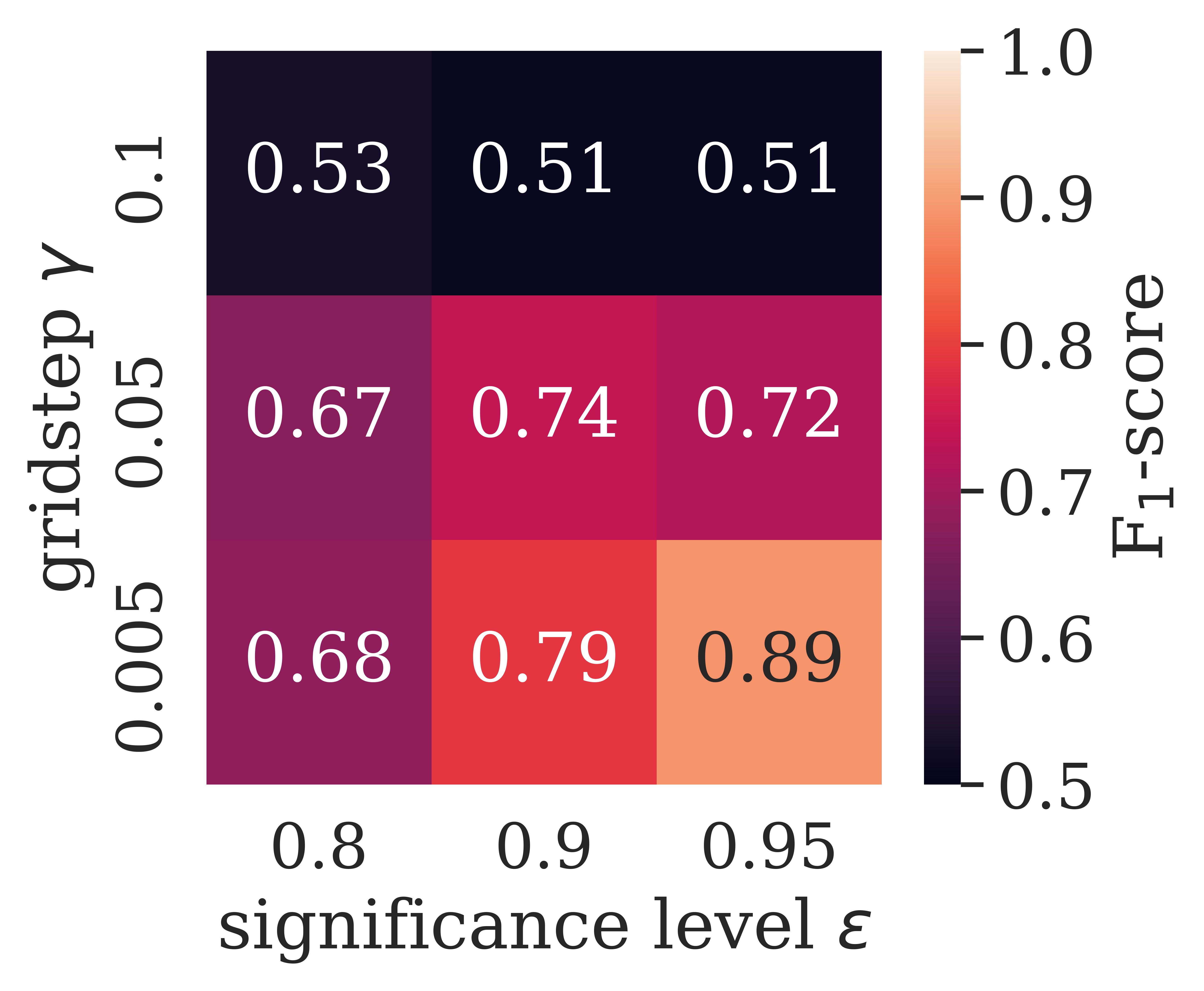
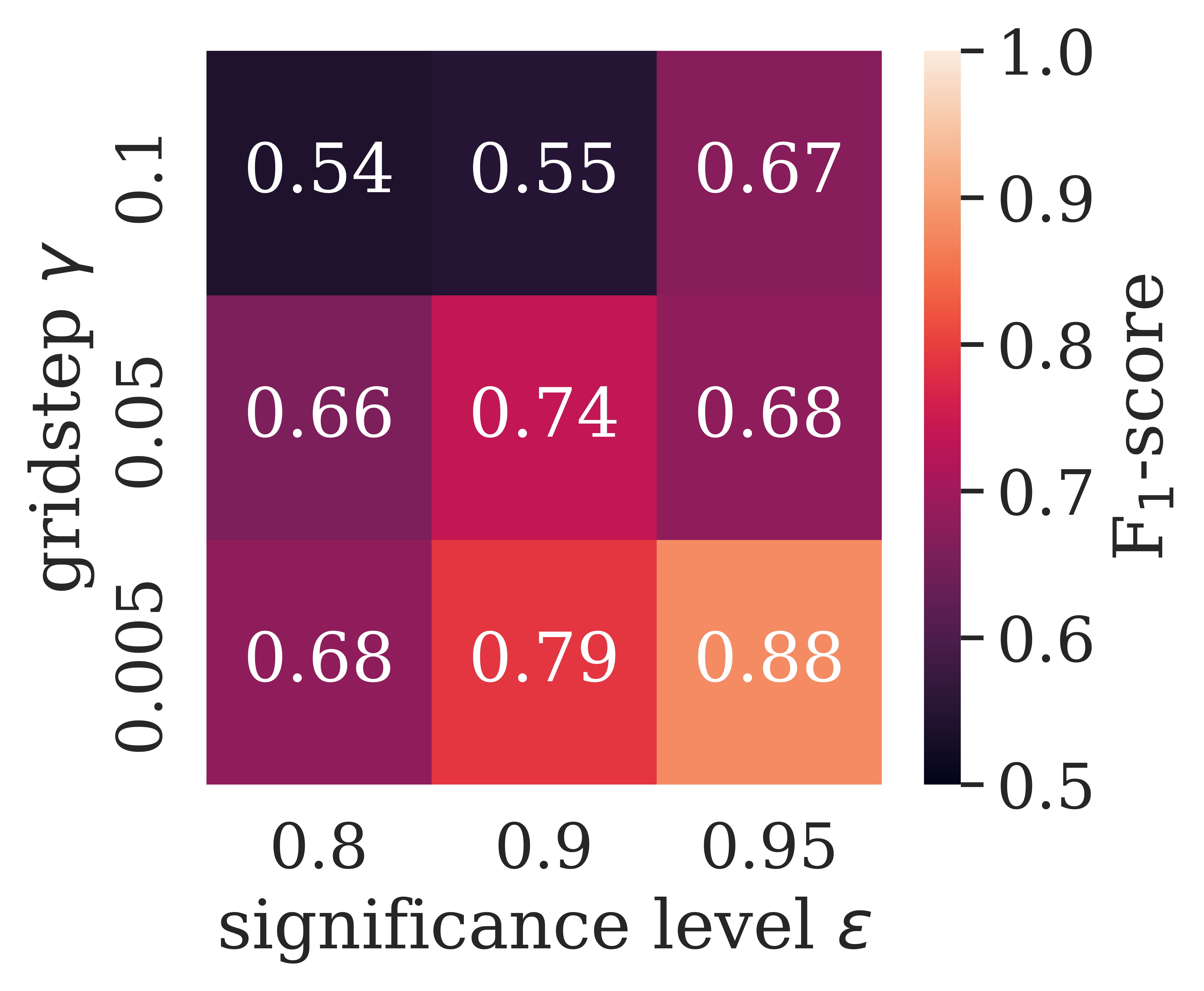
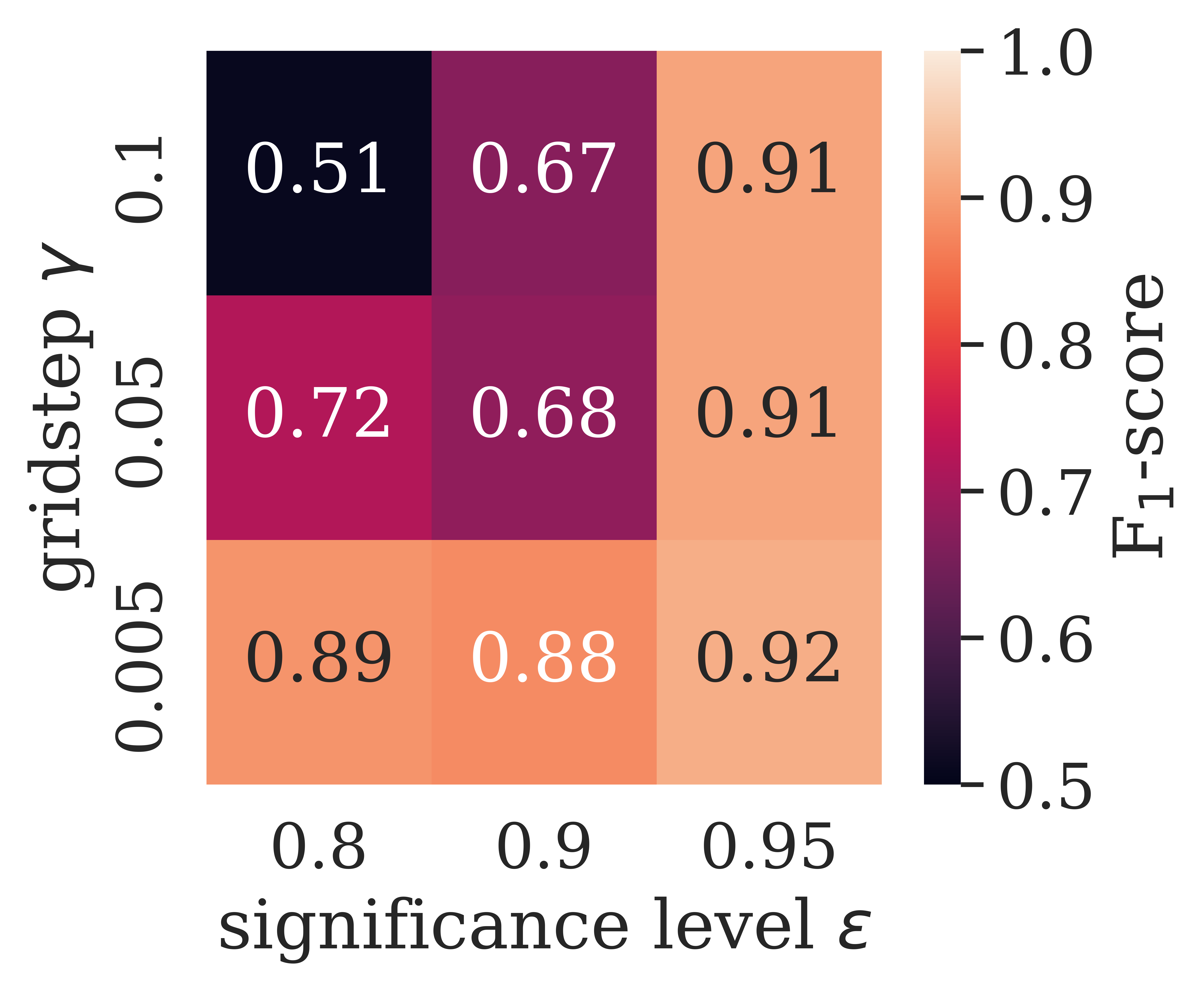
Figure 9 shows a heat map of the F₁-scores achieved by a Deep Learning model trained on the extended dataset Train${}_{\text{ext}}$. Interestingly, we observed a clear pattern with the changing parameters. The results consistently increased with the following:

• A smaller grid step $\gamma$, leading to a higher resolution of the feature space;

• A larger significance level $\epsilon$, which tightens the high-confidence feature space regions;

• And a larger number of original training points $n$, allowing for more precise modelling of the feature space confidence.

Evaluating the results of the optimal extended training set Train${}_{\text{ext}}$ ($\gamma=0.005$, $\epsilon=0.95$) for different sizes of Train${}_{\text{orig}}$, we found that our synthesised results successfully and significantly increased Deep Learning prediction by strengthening the model’s generalisation performance. The F₁-score was increased by 38% for $n=50$ (51% to 89%), by 34% for $n=100$ (59% to 88%), and by 13% for $n=1000$ (from 79% to 92%). The smaller the original dataset, the more impact synthetic samples had. However, the more original samples were available, the higher the best F₁-score could reach. Importantly, there was no detriment to extending a training set with our proposed algorithm. Because of the statistical quality guarantees, Train${}_{\text{ext}}$ set performed at least as well as Train${}_{\text{orig}}$ in the worst-case scenario and significantly better in the best-case scenario.

(a) $n=50$.

(b) $n=100$.

(c) $n=1000$.

Figure 9: Overview of Deep Learning results on the extended training sets synthesised with varying parameters. Each square represents the model’s mean F₁-score on the same original test set. Results followed a similar pattern, improving with smaller grid steps $\gamma$, larger significance levels $\epsilon$, and larger original training sample counts $n$.

Now that we have systematically and comprehensively evaluated a simple toy dataset, we turn to real-world datasets to verify our proposed conformal synthesis algorithm. The following algorithm parameter choices were informed by insights gained in this section.

5.3 Evaluating real-world datasets

To assess the practical benefits of our conformal synthesis algorithm, we tested its application to four realistic benchmark datasets. The datasets were carefully selected to showcase our algorithm’s range on some of the most prevalent data challenges limiting Machine Learning implementations: Low sample count, class imbalance and overlap, and data privacy.

Following the details laid out in Section 5.1, we measured the success of our algorithm by comparing the prediction results of a feedforward neural network trained on the original data Train${}_{\text{orig}}$ and our extended data Train${}_{\text{ext}}$ on the same test set. The optimal parameters for data synthesis were identified in Section 5.2. Note that we use UMAP [46] to reduce all datasets’ dimensions to two features for visualisation purposes. However, our proposed algorithm is compatible with any size dimensional input.

5.3.1 Small dataset

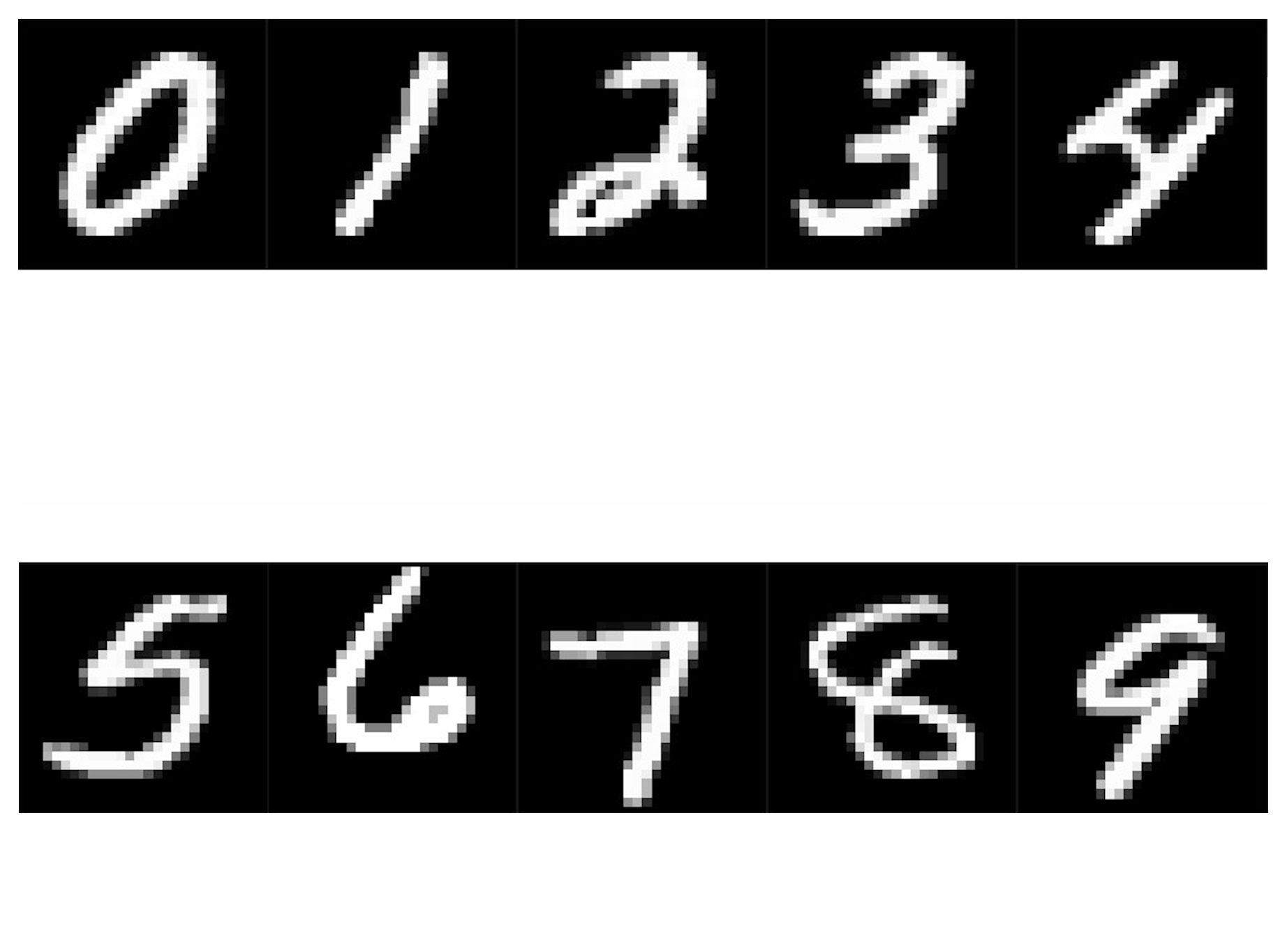
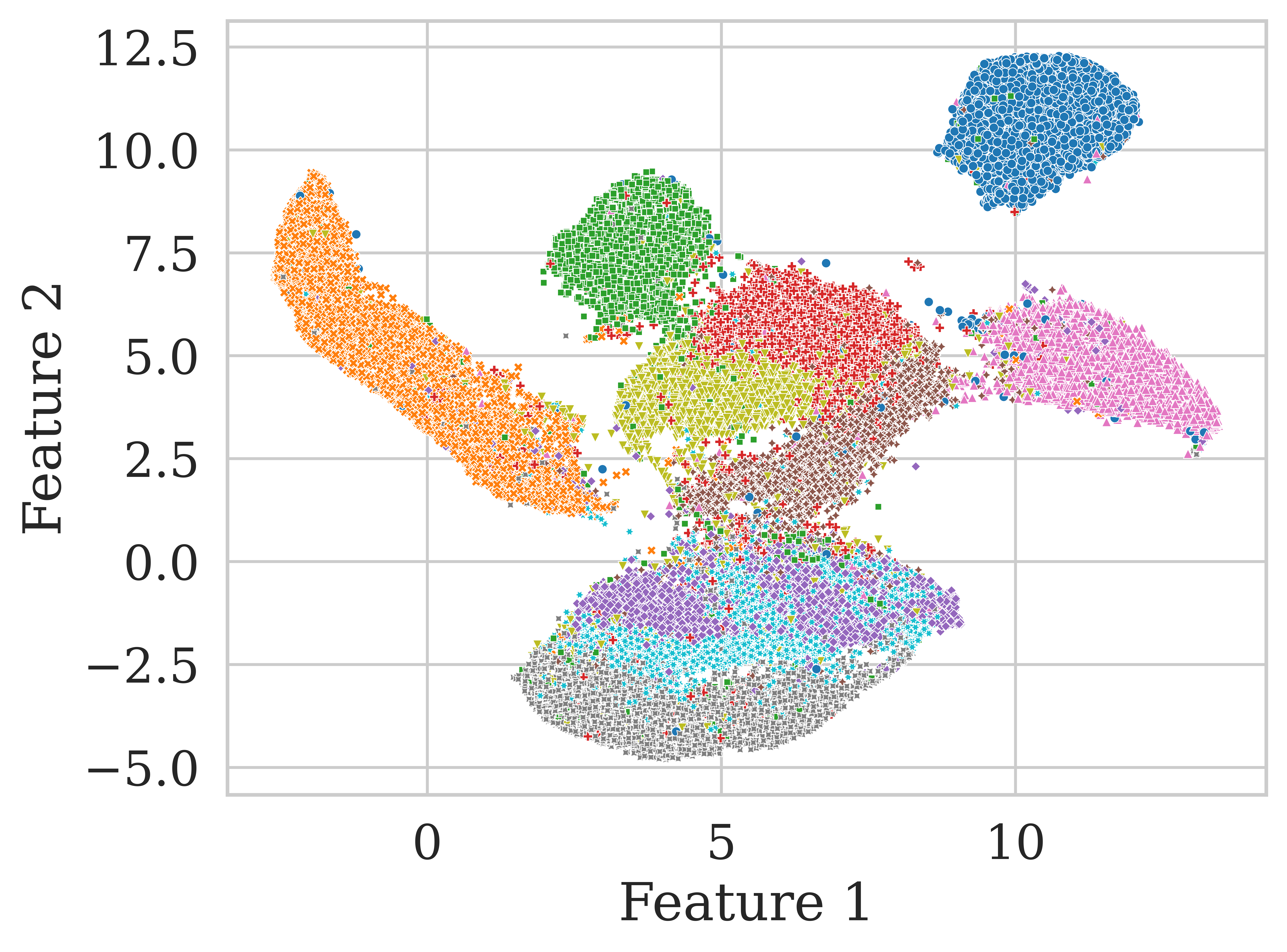
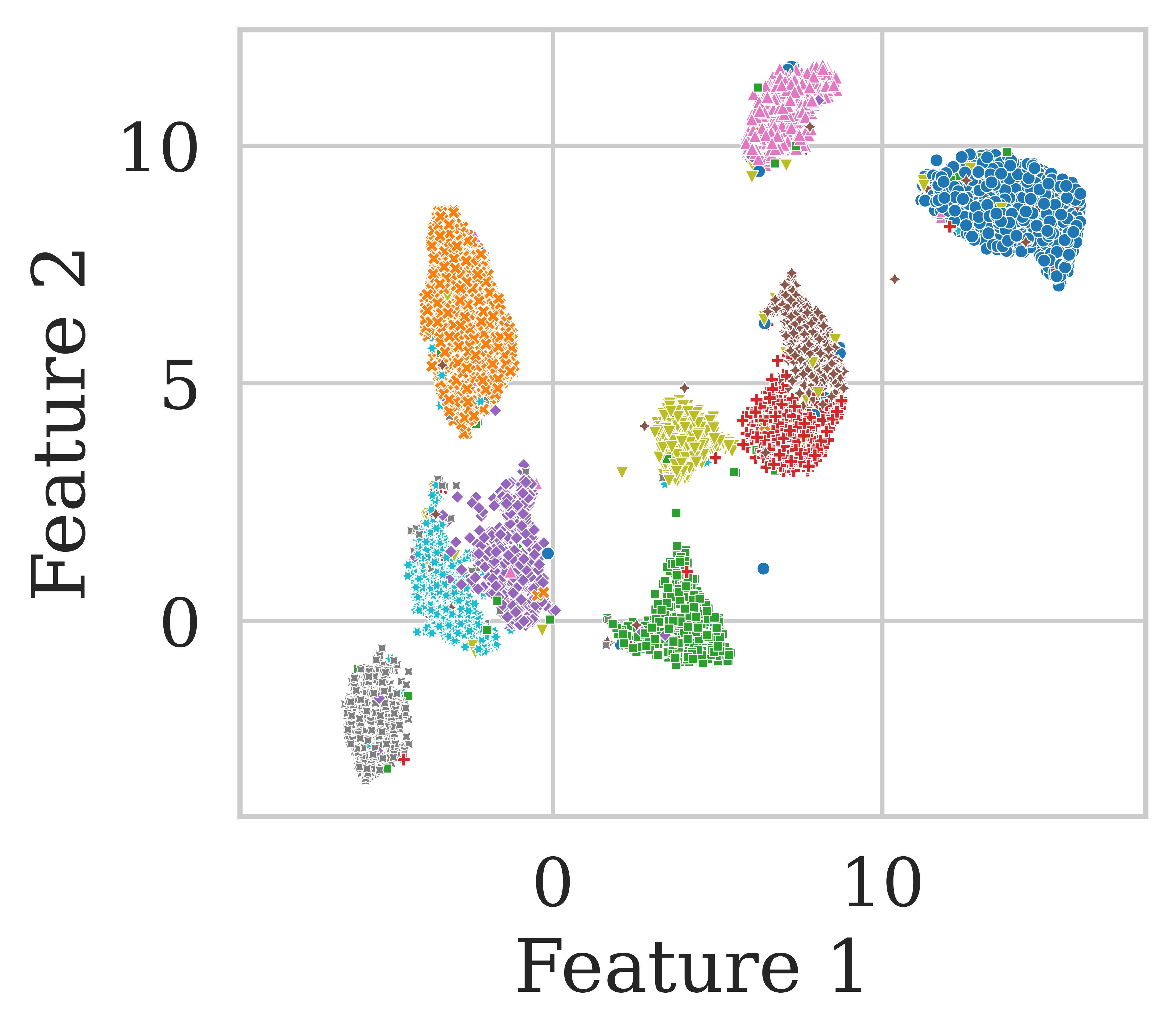
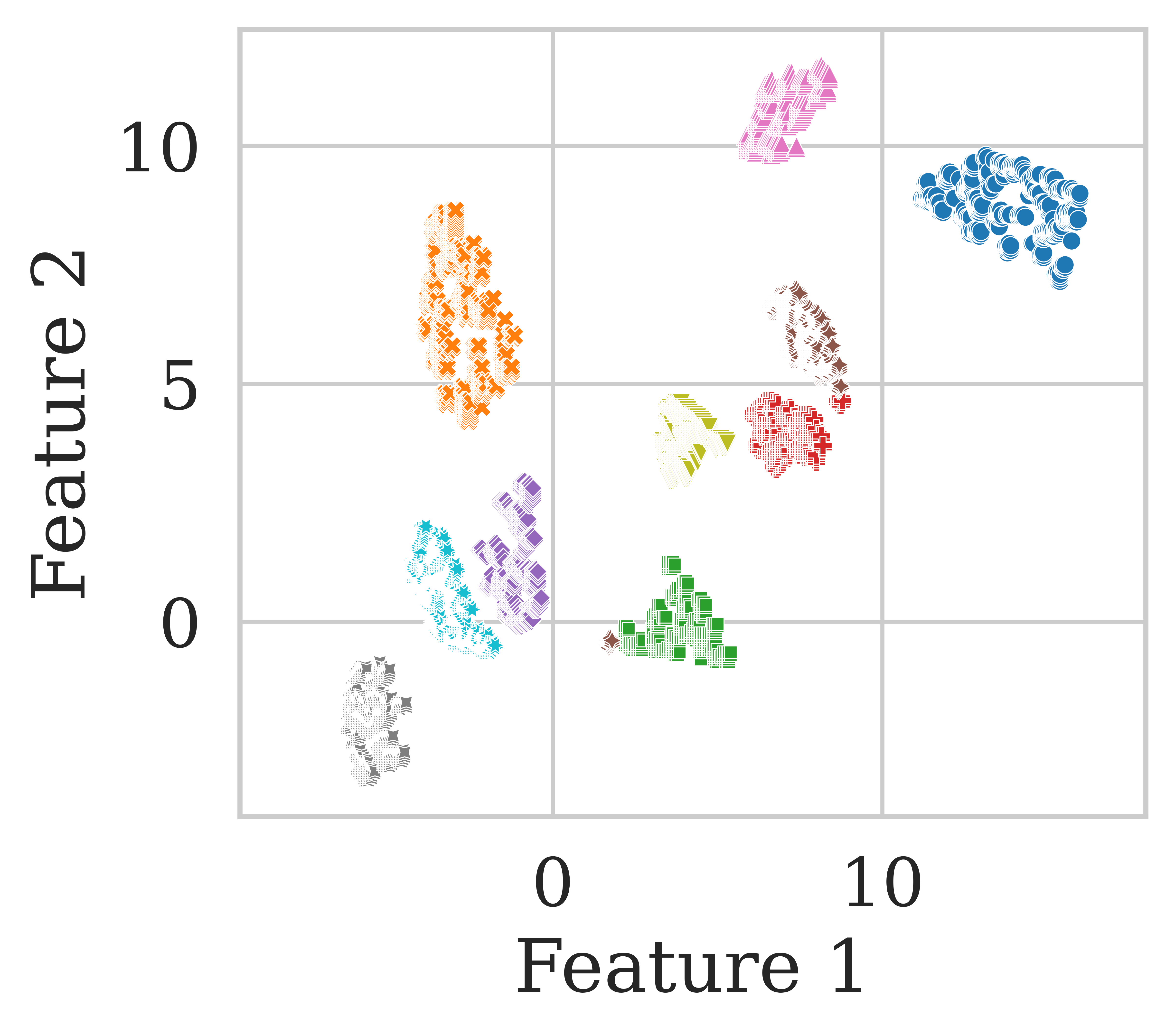
Low sample counts are a ubiquitous challenge in Deep Learning, often caused by the difficulties and costs of data collection. To simulate a low training sample count, we used the popular MNIST dataset [47]. With 70,000 original samples, we could carry out an in-depth investigation of our algorithm’s benefits across a range of dataset sizes. Figure 10(a) presents a selection of samples from the 0–9 handwritten digits contained in the dataset. Each 28x28 pixel image was scaled to $(0,1)$ and reduced to two dimensions to enable 2D visualisation. Figure 10(b) shows the samples’ distribution in the feature space after pre-processing. While some classes are very clearly linearly separated, most are adjacent with limited overlap. Overall, the number of samples is relatively balanced per class.

(a) Handwritten digit samples.

(b) Pre-processed samples.

Figure 10: The MNIST dataset of handwritten digits. Each image was reduced to two dimensions with UMAP before model training. Most classes (differentiated by colour and marker) are adjacent with some overlap, making class separation challenging.

The core purpose of our proposed algorithm is to support Deep Learning generalisation by extending datasets with synthetic training samples. To showcase our approach’s benefits across varying original set-sizes Train${}_{\text{orig}}$, we synthesised new data points for dataset subsets, as shown in Table 4. Generally, the more original training points were available, the smaller the number of synthesised samples was, caused by more precise (and therefore more narrow) confidence regions.

Table 4: Original and synthesised sample counts. The larger the original dataset was, the more narrow and precise the confidence regions were, and the fewer new sample points were synthesised. The conformal parameters $\epsilon=0.95$ and $\gamma=0.005$ were identified in Section 5.2.

Subset	Test	Trainorig	Trainsyn	Trainext
$D_{\mathbf{{300}}}$	10,000	300	1,348,009	1,348,309
$D_{\mathbf{{1000}}}$	10,000	1,000	1,136,407	1,137,407
$D_{\mathbf{{10000}}}$	10,000	10,000	1,828,567	1,838,567
$D_{\mathbf{{60000}}}$	10,000	60,000	1,091,878	1,151,878

Table 5 showcases our results with varying training set sizes. In each trial, we evaluated the mean F₁-score, Precision, and Recall of five models trained on Train${}_{\text{orig}}$ and Train${}_{\text{ext}}$ on the same original test set. Starting with the original training samples, the models performed very poorly on low training sample counts as expected (under 30% F₁-score for D₃₀₀ and D₁₀₀₀). The score increased up to 82% with the maximum number of training samples (D₆₀₀₀₀). In contrast, our synthetic dataset extension surpassed that performance from 1,000 original training samples. With only 300 original samples, our algorithm synthesised samples that improved model performance from 17% to 79% F₁-score. While the rate of improvement decreased with increasing training samples, our extended Train${}_{\text{ext}}$ consistently outperformed all Train${}_{\text{orig}}$, reaching a maximum of 84% on the full dataset. Because the classes were roughly equally balanced in the original dataset, this increase was caused by Precision and Recall improving in equal measure.

Table 5: MNIST mean Deep Learning results with varying Train${}_{\text{orig}}$ size. We report the mean performance across five trials. As the number of original samples increased, so did the models’ performance, although at different rates. The Precision and Recall scores stayed level with each other, implying that synthesis successfully maintained the class’ original balance.

	F1-score		Precision		Recall
Subset	Trainorig	Trainext	Trainorig	Trainext	Trainorig	Trainext
$D_{\mathbf{{300}}}$	0.17 (0.05)	0.79 (0.01)	0.17 (0.04)	0.80 (0.00)	0.25 (0.08)	0.80 (0.00)
$D_{\mathbf{{1000}}}$	0.26 (0.04)	0.83 (0.00)	0.27 (0.04)	0.83 (0.00)	0.36 (0.04)	0.82 (0.00)
$D_{\mathbf{{10000}}}$	0.76 (0.04)	0.83 (0.01)	0.76 (0.01)	0.84 (0.01)	0.74 (0.02)	0.83 (0.01)
$D_{\mathbf{{60000}}}$	0.82 (0.00)	0.84 (0.00)	0.84 (0.01)	0.84 (0.00)	0.83 (0.00)	0.84 (0.00)

From these results, we deduce that our synthesis algorithm can successfully identify high-confidence class regions of the feature space with very few original training samples. So few, in fact, that a neural network could not robustly identify class patterns without extension. This makes our proposal highly advantageous for Deep Learning, as its synthesised samples allow for significantly improved model generalisation without requiring additional data collection.

5.3.2 Imbalanced data

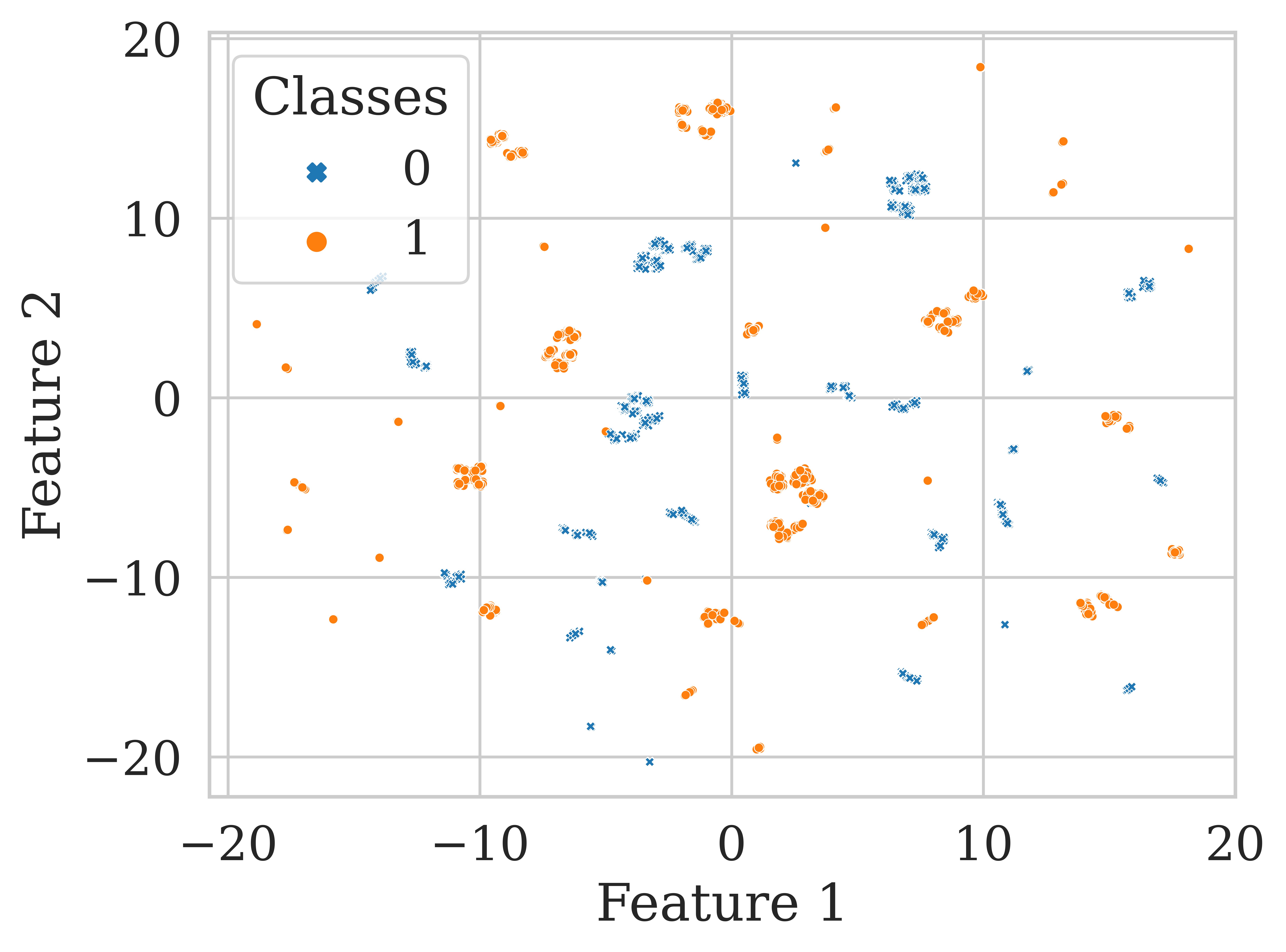
Class imbalances are a frequent and often inevitable occurrence in real-world datasets due to the underlying population’s unequal distribution (e.g., healthy vs disease). Even if the total number of available samples is large, the minority class’s under-representation may lead to skewed results. To illustrate the effects of imbalance on model performance and the combating benefits of our data synthesis algorithm, we use the MSHRM benchmark dataset [48]. MSHRM contains records of around 5,500 samples separated into edible (class 0) and poisonous (class 1) mushrooms. The pre-processing steps include replacing categorical variables with dummies and reducing the samples to two dimensions with UMAP (Figure 11).

Figure 11: The MSHRM dataset. Originally roughly equally distributed, we artificially sub-sample the data to simulate class imbalances of varying severity for synthesis (Table 6).

Once again, we simulated different levels of class imbalance by sub-sampling the original dataset (1:1, 1:2, 1:4, 1:10). Table 6 contains the tested subsets and their per-class sample counts. Worth noting is that the level of imbalance has a drastic impact on the number and class distribution of our synthetic samples, far out-reaching the class ratio of Train${}_{\text{orig}}$ (e.g., $D_{1:9}$ with 1:9 original vs 1:1310 synthetic samples).

Table 6: MSHRM sample counts with varying imbalance, differentiated by class. The original data’s imbalance significantly impacted the balance of the synthetic samples. The larger the imbalance was, the more samples were synthesised for the minority class.

	Test	Trainorig			Trainsyn			Trainext
Subset	$\mathbf{\sum}$	0	1	$\mathbf{\sum}$	0	1	$\mathbf{\sum}$	0	1	$\mathbf{\sum}$
$D_{\mathbf{{1:1}}}$	2,681	2,613	2,830	5,443	958	996	1,954	3,571	3,826	7,397
$D_{\mathbf{{1:2}}}$	2,681	1,392	2,827	4,219	1,939	665	2,604	3,331	3,492	6,823
$D_{\mathbf{{1:4}}}$	2,681	708	2,831	3,539	10,884	283	11,167	11,592	3,114	14,706
$D_{\mathbf{{1:9}}}$	2,681	314	2,829	3,143	363,101	277	363,378	363,415	3,106	366,521

(a) Train${}_{\text{orig}}$.

(b) Train${}_{\text{ext}}$.

Figure 12: Mean Deep Learning performance on the MSHRM dataset with varying class imbalance. Performance on the original dataset decreased significantly with increasing imbalance. Conversely, performance improved on the extended training set because the number of synthetic samples increased exponentially (Table 6).

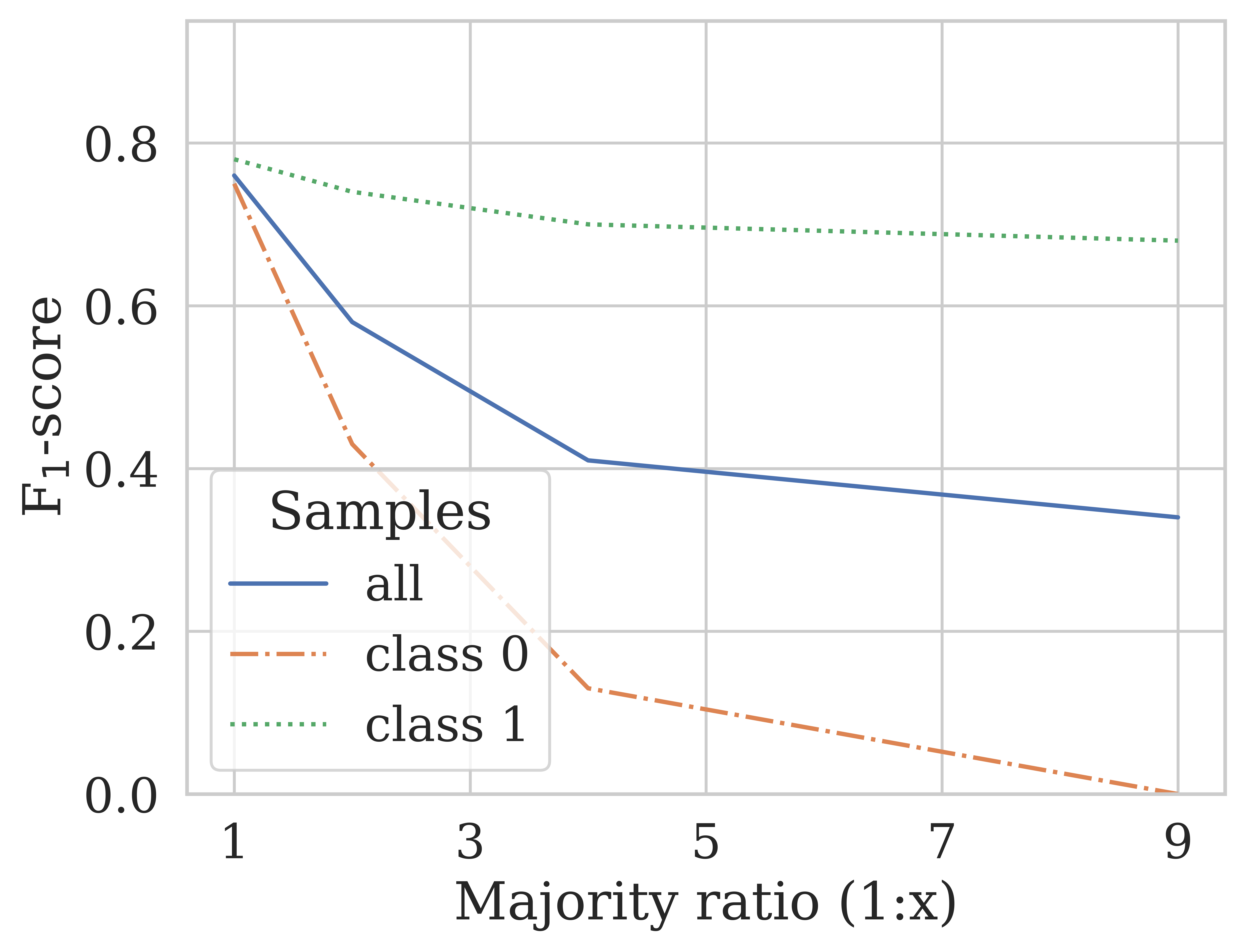
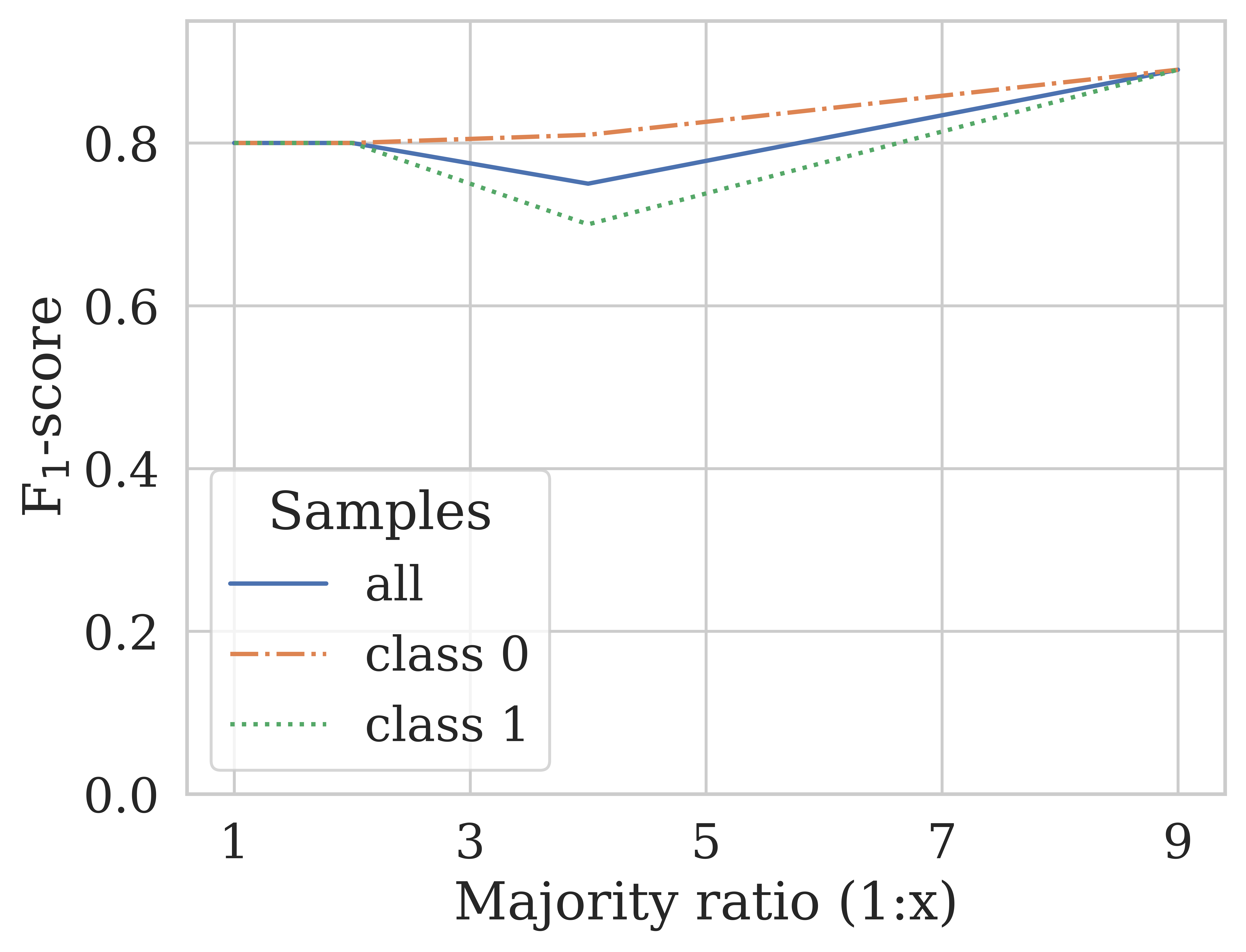
The Deep Learning results are shown in Figure 12. As expected, model performance on Train${}_{\text{orig}}$ decreased severely with the increasing imbalance (76%–34%), mainly due to the F₁-score on the minority class 0, which drops from 75% to 0%. In contrast, the model’s overall F₁-score increased with a larger class imbalance from 80% to 89%. To understand this surprising trend, we refer back to Table 6. The likely cause is that the number of synthetic samples Train${}_{\text{syn}}$ generated for the largest imbalance $D_{1:9}$ was about 150 times larger than when the classes were balanced ($D_{1:1}$). Interestingly, even though the synthetic samples reintroduced the class imbalance (albeit with class 1 now as the majority class), the imbalance was not represented in the final F₁-score (89% overall and per class).

Further investigating this tendency in Table 7, we examined the results of synthesising samples for both classes (Train${}_{\text{ext}}$), compared to only extending the minority class 0 (Train${}_{\text{ext0}}$). Consistently, we found that over-supporting the minority class with synthetic samples did not have the same negative performance impacts as the original imbalance had. In fact, with larger imbalances ($D_{1:4}$, $D_{1:9}$), extending the minority class benefited the overall mean F₁-score by 1–4%.

Table 7: MSHRM mean Deep Learning results with varying class imbalance. We report the mean F₁-score of five trials. Using the synthetic samples in training improved the overall performance significantly, reaching a maximum increase when the imbalance was the largest. The conformal synthesis parameters $\epsilon=0.95$ and $\gamma=0.005$ were identified in Section 5.2.

		F1-score
Class	Subset	Trainorg	Trainext	Trainext0
0 and 1	$D_{\mathbf{{1:1}}}$	0.76 (0.05)	0.80 (0.05)	0.73 (0.09)
	$D_{\mathbf{{1:2}}}$	0.58 (0.03)	0.80 (0.05)	0.78 (0.08)
	$D_{\mathbf{{1:4}}}$	0.41 (0.10)	0.75 (0.11)	0.78 (0.03)
	$D_{\mathbf{{1:9}}}$	0.34 (0.00)	0.89 (0.01)	0.90 (0.01)
0	$D_{\mathbf{{1:1}}}$	0.75 (0.07)	0.80 (0.05)	0.78 (0.04)
	$D_{\mathbf{{1:2}}}$	0.43 (0.05)	0.80 (0.06)	0.79 (0.07)
	$D_{\mathbf{{1:4}}}$	0.13 (0.17)	0.81 (0.06)	0.81 (0.02)
	$D_{\mathbf{{1:9}}}$	0.00 (0.00)	0.89 (0.01)	0.90 (0.01)
1	$D_{\mathbf{{1:1}}}$	0.78 (0.04)	0.80 (0.05)	0.68 (0.14)
	$D_{\mathbf{{1:2}}}$	0.74 (0.01)	0.80 (0.04)	0.76 (0.09)
	$D_{\mathbf{{1:4}}}$	0.70 (0.02)	0.70 (0.15)	0.74 (0.04)
	$D_{\mathbf{{1:9}}}$	0.68 (0.00)	0.89 (0.02)	0.90 (0.01)

5.3.3 Overlapping classes

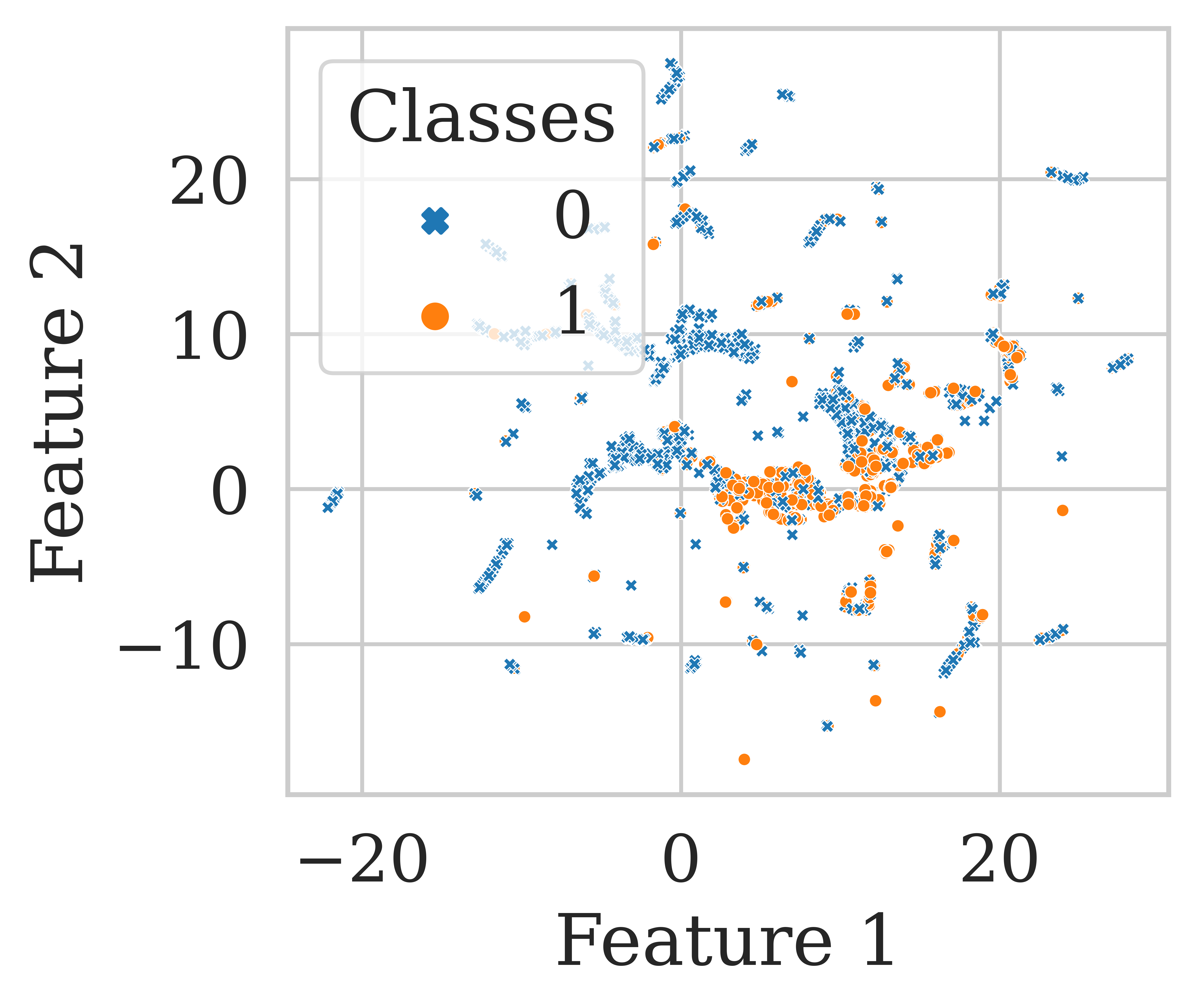
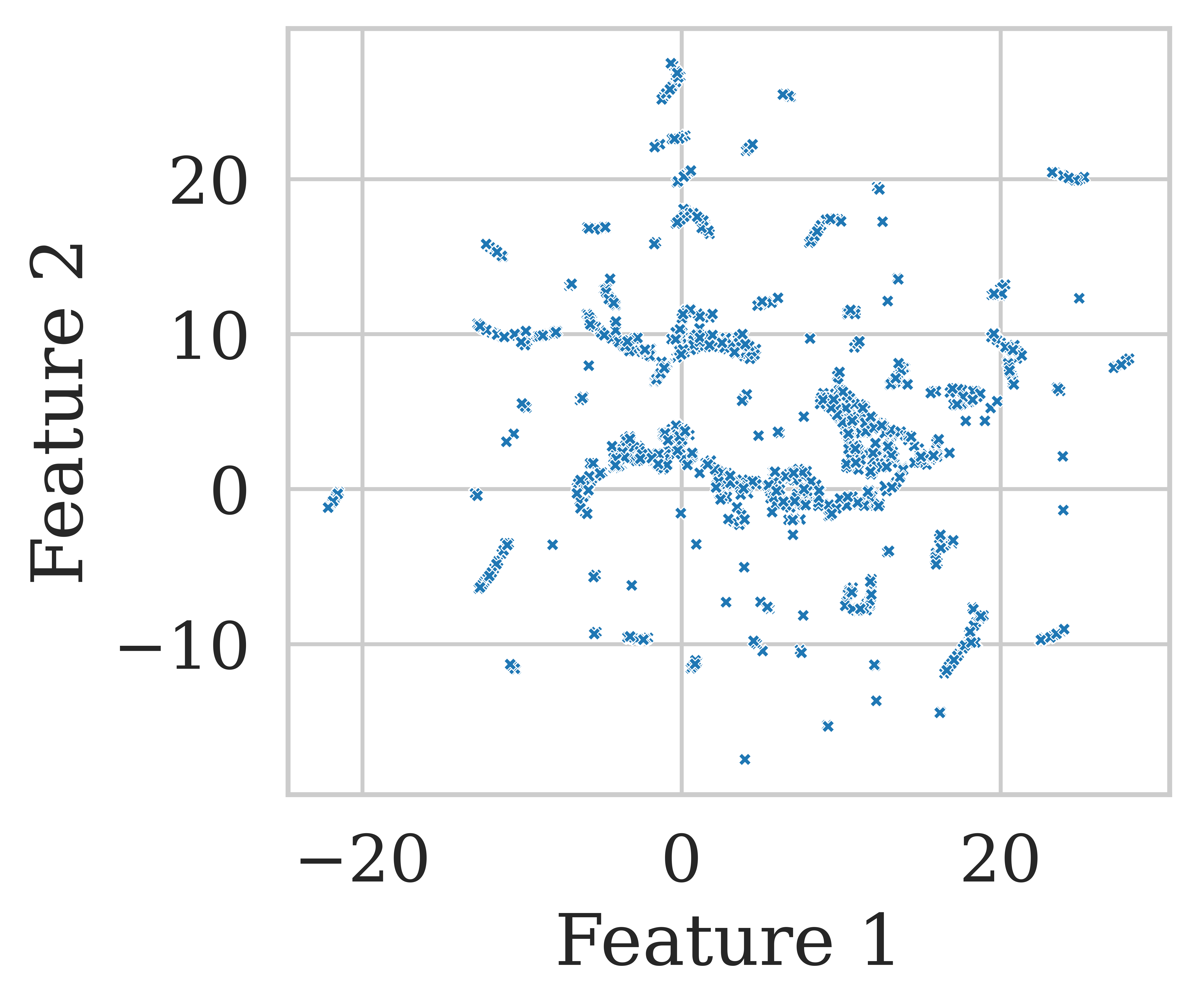
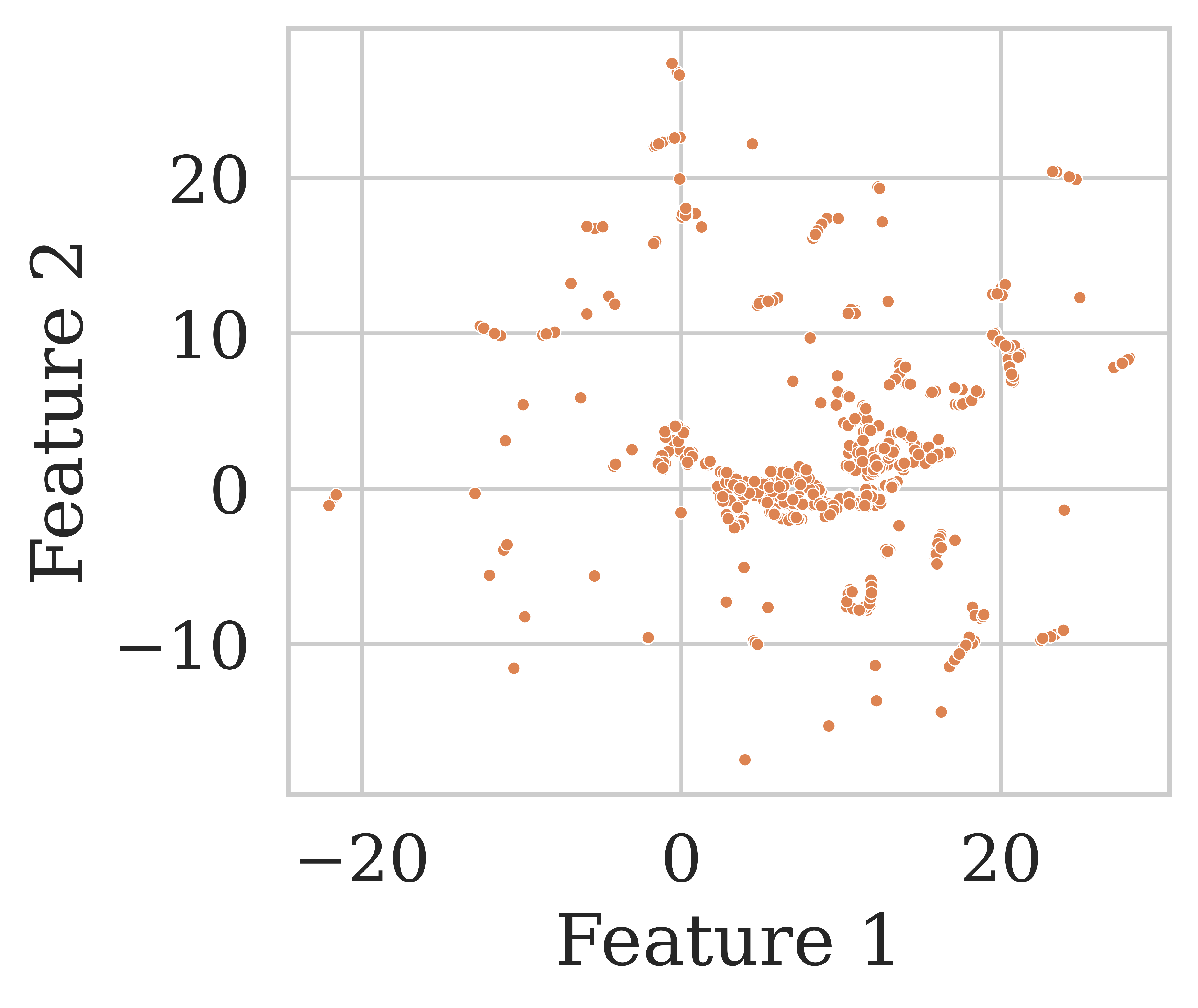
Deep Learning modelling of prediction tasks relies on the separability of the classes. However, real-world datasets often do not have clear separation due to sample noise and uninformative features. We demonstrate the advantages of our proposed algorithm in these cases on the WINE benchmark dataset [49], where we classify whether a sample represents white (class 0) or red (class 1) wine based on chemical measurements. As shown in Figure 13, this “difficult” dataset has no class separability, with both classes overlapping quite significantly in the feature space. Consequently, the high-confidence regions for data synthesis overlap as well. Because of its difficulty, we encourage a larger set of synthetic samples by lowering $\epsilon$ from $0.95$ to $0.9$. Table 8 records the evaluated original and synthetic sample counts.

(a) All classes.

(b) Class 0.

(c) Class 1.

Figure 13: The WINE dataset shows significant class overlap in the feature space. Consequently, the high-confidence regions identified by our synthesis algorithm were also overlapped. The non-separability of the classes made accurate predictions challenging.

Table 8: WINE original and synthetic sample counts. While synthesis generally maintains the class’s non-separability, significantly increasing the number of available training samples may nonetheless support Deep Learning generalisation. Therefore, the significance level $\epsilon$ was reduced to 0.9 to encourage additional synthetic samples by widening the confidence regions ($\gamma=0.005$).

Subset	Test	Trainorig	Trainsyn	Trainext
$D\mathbf{{}_{orig}}$	2,145	4,352	—	—
$D\mathbf{{}_{ext}}$	2,145	4,352	130,693	135,045

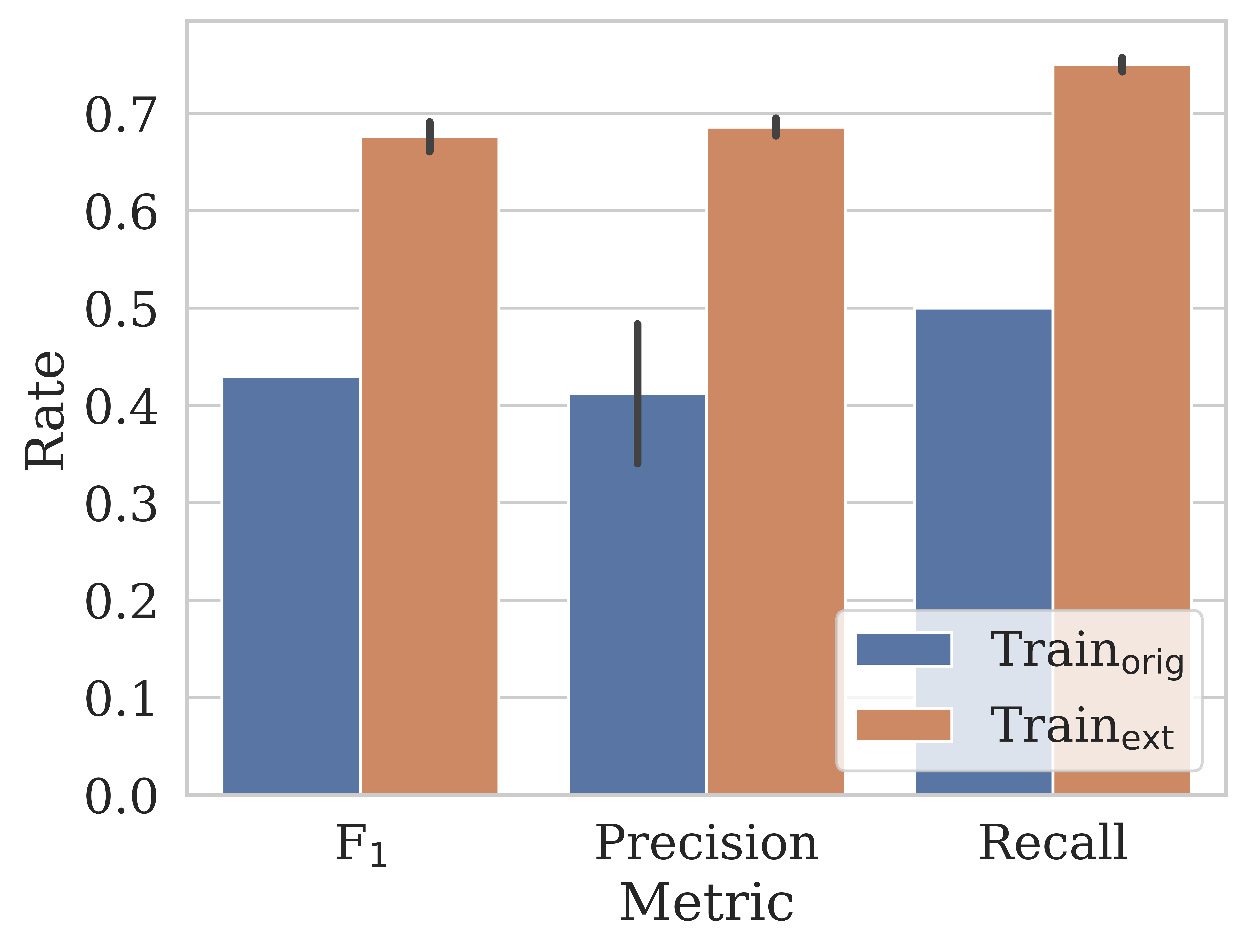
Figure 14 visualises the performance of five models trained on the original Train${}_{\text{orig}}$ and the extended Train${}_{\text{ext}}$ datasets. Compared to the 43% F₁-score achieved on the original data, including the synthesised data for training increases the performance by 25% to a total of 68%. Precision and Recall confirm that the model’s ability to identify relevant samples was strengthened. In summary, even though our proposed algorithm did not increase the linear separability of the classes, it nonetheless significantly improved the model’s performance. The model’s learning was supported through the synthesis of a large number of new training samples.

Figure 14: Mean Deep Learning performance on the WINE dataset. The error bars show the standard deviation. Even though synthesis did not improve the classes’ separability, the large quantity of additional samples significantly improved the models’ generalisation.

5.3.4 Synthetic replacement

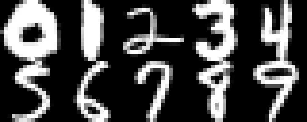
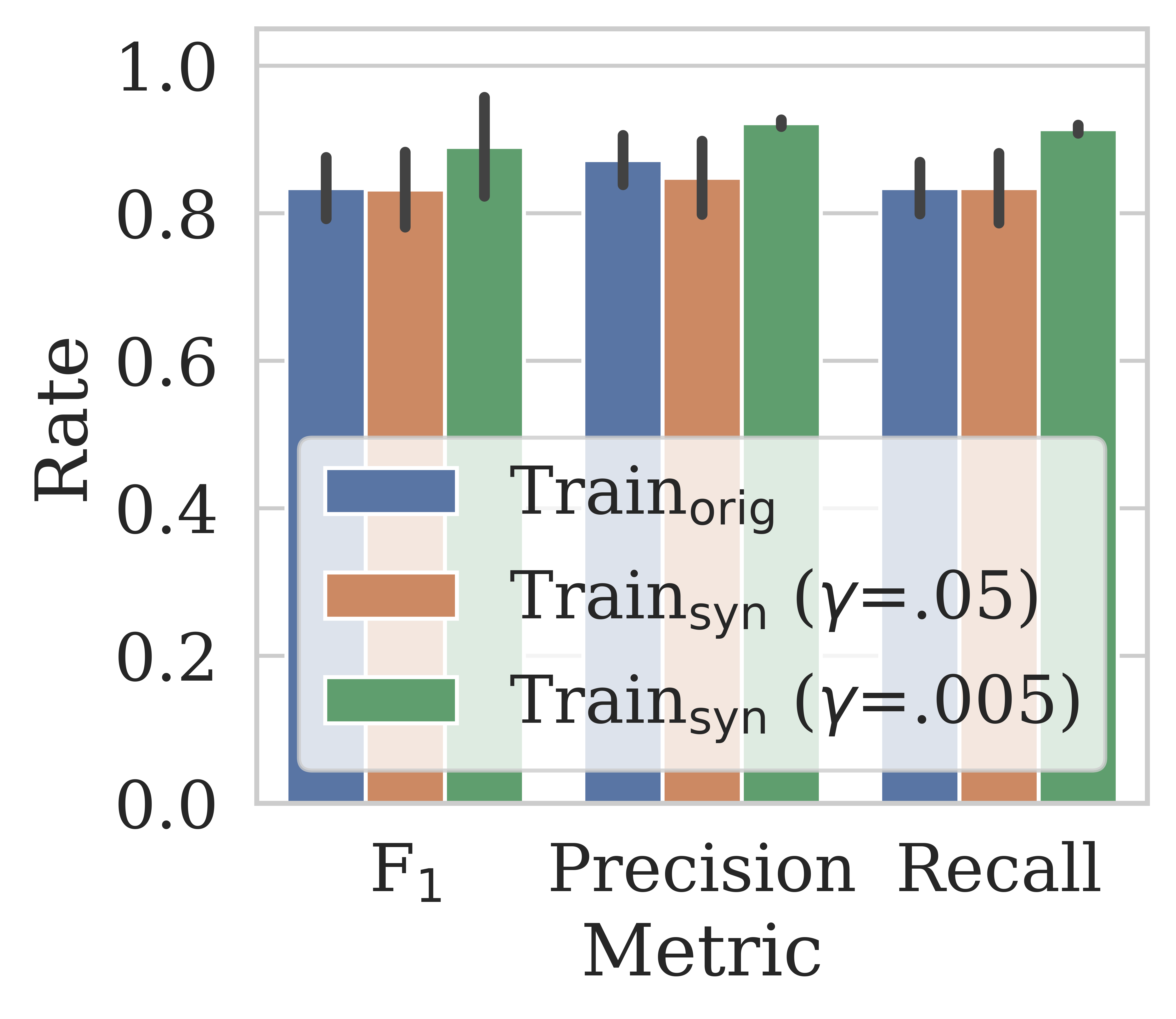
As a final show of our algorithm’s ability to accurately synthesise new samples, we tested a full synthetic replacement of the original dataset for Deep Learning training. This type of synthesis has many real-world applications, for example to maintain data privacy when publicly releasing sensitive data. The experiments were carried out on the USPS dataset of digits scanned from envelopes by the U.S Postal Service [50], shown in Figure 15. We evaluated two synthetic datasets: One of a roughly similar size as the original and one with the number of samples increased 10-fold. The original and synthetic sample counts are listed in Table 9.

Figure 16 summarises the results of the full synthetic replacement. Both synthetic training sets ($\gamma=0.05,0.005$) performed at least as well as Train${}_{\text{orig}}$ on the original test set. With the decrease of $\gamma$ to 0.005, we achieved an even higher score, raising the mean F₁-score by 6%, from 83% to 89%. Precision and Recall indicate that our synthesis algorithm preserved the original classes’ balance, allowing models trained on the synthetic datasets to maintain or strengthen their ability to identify relevant samples.

Figure 15: USPS handwritten digits dataset. Each sample contains one grey-scale digit in a 16x16 format.

Table 9: Original and synthetic sample counts of the USPS dataset. We tested two scenarios of full synthetic replacement: One of roughly similar size and one with significantly increased sample counts. The size of Train${}_{\text{syn}}$ was controlled by varying the grid step $\gamma$ ($\epsilon=0.95$).

Subset	$\mathbf{\gamma}$	Test	Trainorig	Trainsyn
$D_{\mathbf{{orig}}}$	—	2,007	7,291	—
$D_{\mathbf{{0.05}}}$	0.05	2,007	7,291	5,694
$D_{\mathbf{{0.005}}}$	0.005	2,007	7,291	569,711

(a) Train${}_{\text{orig}}$ points per class.

(b) Train${}_{\text{syn}}$ points per class.

(c) DL results.

Figure 16: USPS results of two full synthetic replacements, one of roughly the same size as the original dataset ($\gamma=0.05$), and one increased 10-fold ($\gamma=0.005$). The mean and standard deviation Deep Learning results of five iterations are reported. The models trained on the synthetic data matched or improved performance, indicating that our conformal algorithm successfully maintained the samples’ distribution and strengthened the learned representations.

6 Conclusion and future work

In conclusion, we have presented a unique conformal data synthesis algorithm that introduces statistical guarantees to the data generation process. Limiting our data synthesis to high-confidence regions of the feature space guarantees the synthetic data’s quality to a user-specified significance level. Based on the foundational Conformal Predication framework, we supported our novel proposal with theoretical proofs. Additionally, we presented comprehensive empirical results on five benchmark datasets, demonstrating our algorithm’s advantages for a variety of ubiquitous real-world challenges:

• Synthesising high-quality data to significantly boost the sample size of small datasets, as well as correcting class imbalances,

• Supporting a model’s learned feature space representations of non-separable classes,

• And replacing an entire dataset with synthetic samples to preserve data privacy, maintaining the data’s distribution for Deep Learning performance.

While our proposed algorithm is capable of synthesising any data with high quality, generating associated ground truths is currently limited to classification labels and may be an interesting avenue for further extension. Additionally, examining the effects of different non-conformity measures used to evaluate confidence may lead to further performance improvements in the future.

Declarations

• Competing interests: The authors declare that they have no conflict of interest.

• Funding: No funding was received for conducting this study.

• Author contributions: All authors contributed to the study’s conception and design. J.M. carried out the experimentation, performed the analysis, and drafted the manuscript under K.N.’s supervision. All authors critically reviewed and approved the final manuscript.

• Availability of data and materials: The benchmark datasets evaluated in this article are available from the UCI Machine Learning repository (MNIST dataset [51], Mushroom dataset [52], Wine dataset [53]) and from Kaggle (USPS dataset [54]).

• Code availability: The implementation and results are available at https://github.com/juliameister/conformal-data-synthesis.

References

- \bibcommenthead
- Brigato and Iocchi [2021] Brigato, L., Iocchi, L.: A close look at Deep Learning with small data. In: 2020 25th International Conference on Pattern Recognition (ICPR), pp. 2490–2497. IEEE, New York (2021). https://doi.org/10.1109/ICPR48806.2021.9412492 . https://ieeexplore.ieee.org/document/9412492/
- Moreno-Barea et al. [2020] Moreno-Barea, F.J., Jerez, J.M., Franco, L.: Improving classification accuracy using data augmentation on small data sets. Expert Systems with Applications 161(0957-4174), 113696 (2020) https://doi.org/10.1016/j.eswa.2020.113696
- Sarker [2021] Sarker, I.H.: Deep Learning: A comprehensive overview on techniques, taxonomy, applications and research directions. SN Computer Science 2(6), 420 (2021) https://doi.org/10.1007/s42979-021-00815-1
- Zhuang et al. [2019] Zhuang, P., Schwing, A.G., Koyejo, O.: FMRI data augmentation via synthesis. In: 2019 IEEE 16th International Symposium on Biomedical Imaging (ISBI 2019), vol. 2019-April, pp. 1783–1787. IEEE, New York (2019). https://doi.org/10.1109/ISBI.2019.8759585 . https://ieeexplore.ieee.org/document/8759585/
- Liu et al. [2022] Liu, S., Jiang, H., Wu, Z., Li, X.: Data synthesis using deep feature enhanced Generative Adversarial Networks for rolling bearing imbalanced fault diagnosis. Mechanical Systems and Signal Processing 163, 108139 (2022) https://doi.org/10.1016/j.ymssp.2021.108139
- Shafer and Vovk [2008] Shafer, G., Vovk, V.: A tutorial on Conformal Prediction. Journal of Machine Learning Research 9(3), 371–421 (2008)
- Cherubin et al. [2015] Cherubin, G., Nouretdinov, I., Gammerman, A., Jordaney, R., Wang, Z., Papini, D., Cavallaro, L.: Conformal clustering and its application to botnet traffic. In: 2015 Statistical Learning and Data Sciences (SLDS): Lecture Notes in Computer Science, vol. 9047, pp. 313–322. Springer, Cham (2015). https://doi.org/10.1007/978-3-319-17091-6_26 . https://link.springer.com/10.1007/978-3-319-17091-6_26
- Li et al. [2020] Li, Q., Zheng, Z., Wu, F., Chen, G.: Generative Adversarial Networks-based privacy-preserving 3D reconstruction. In: 2020 IEEE/ACM 28th International Symposium on Quality of Service (IWQoS), pp. 1–10. IEEE, New York (2020). https://doi.org/10.1109/IWQoS49365.2020.9213037 . https://ieeexplore.ieee.org/document/9213037/
- Yoon et al. [2020] Yoon, J., Drumright, L.N., Schaar, M.: Anonymization through data synthesis using Generative Adversarial Networks (ADS-GAN). IEEE Journal of Biomedical and Health Informatics 24(8), 2378–2388 (2020) https://doi.org/10.1109/JBHI.2020.2980262
- Thambawita et al. [2021] Thambawita, V., Isaksen, J.L., Hicks, S.A., Ghouse, J., Ahlberg, G., Linneberg, A., Grarup, N., Ellervik, C., Olesen, M.S., Hansen, T., Graff, C., Holstein-Rathlou, N.-H., Strümke, I., Hammer, H.L., Maleckar, M.M., Halvorsen, P., Riegler, M.A., Kanters, J.K.: DeepFake electrocardiograms using Generative Adversarial Networks are the beginning of the end for privacy issues in medicine. Scientific Reports 11(1), 21896 (2021) https://doi.org/10.1038/s41598-021-01295-2
- Muramatsu et al. [2020] Muramatsu, C., Nishio, M., Goto, T., Oiwa, M., Morita, T., Yakami, M., Kubo, T., Togashi, K., Fujita, H.: Improving breast mass classification by shared data with domain transformation using a Generative Adversarial Network. Computers in Biology and Medicine 119, 103698 (2020) https://doi.org/10.1016/j.compbiomed.2020.103698
- Salazar et al. [2021] Salazar, A., Vergara, L., Safont, G.: Generative Adversarial Networks and Markov Random Fields for oversampling very small training sets. Expert Systems with Applications 163, 113819 (2021) https://doi.org/10.1016/j.eswa.2020.113819
- Koshino et al. [2021] Koshino, K., Werner, R.A., Pomper, M.G., Bundschuh, R.A., Toriumi, F., Higuchi, T., Rowe, S.P.: Narrative review of Generative Adversarial Networks in medical and molecular imaging. Annals of Translational Medicine 9(9), 821–821 (2021) https://doi.org/10.21037/atm-20-6325
- Bashir et al. [2020] Bashir, D., Montañez, G.D., Sehra, S., Segura, P.S., Lauw, J.: An information-theoretic perspective on overfitting and underfitting. In: AI 2020: AI 2020: Advances in Artificial Intelligence vol. 12576 LNAI, pp. 347–358. Springer, Cham (2020). https://doi.org/10.1007/978-3-030-64984-5_27 . https://link.springer.com/10.1007/978-3-030-64984-5_27
- Bejani and Ghatee [2021] Bejani, M.M., Ghatee, M.: A systematic review on overfitting control in shallow and deep Neural Networks. Artificial Intelligence Review 54(8), 6391–6438 (2021) https://doi.org/10.1007/s10462-021-09975-1
- Whang et al. [2023] Whang, S.E., Roh, Y., Song, H., Lee, J.-G.: Data collection and quality challenges in Deep Learning: A data-centric AI perspective. The VLDB Journal 32(4), 791–813 (2023) https://doi.org/10.1007/s00778-022-00775-9
- Goodfellow et al. [2020] Goodfellow, I., Pouget-Abadie, J., Mirza, M., Xu, B., Warde-Farley, D., Ozair, S., Courville, A., Bengio, Y.: Generative Adversarial Networks. Communications of the ACM 63(11), 139–144 (2020) https://doi.org/10.1145/3422622 arXiv:1406.2661
- Kammoun et al. [2022] Kammoun, A., Slama, R., Tabia, H., Ouni, T., Abid, M.: Generative Adversarial Networks for face generation: A survey. ACM Computing Surveys 55(5), 1–37 (2022) https://doi.org/10.1145/3527850
- Borji [2022] Borji, A.: Pros and cons of GAN evaluation measures: New developments. Computer Vision and Image Understanding 215, 103329 (2022) https://doi.org/10.1016/j.cviu.2021.103329
- Navidan et al. [2021] Navidan, H., Moshiri, P.F., Nabati, M., Shahbazian, R., Ghorashi, S.A., Shah-Mansouri, V., Windridge, D.: Generative Adversarial Networks (GANs) in networking: A comprehensive survey and evaluation. Computer Networks 194, 108149 (2021) https://doi.org/10.1016/j.comnet.2021.108149 arXiv:2105.04184
- Brophy et al. [2023] Brophy, E., Wang, Z., She, Q., Ward, T.: Generative Adversarial Networks in time series: A systematic literature review. ACM Computing Surveys 55(10), 1–31 (2023) https://doi.org/10.1145/3559540
- Saxena and Cao [2022] Saxena, D., Cao, J.: Generative Adversarial Networks (GANs): Challenges, solutions, and future directions. ACM Computing Surveys 54(3), 1–42 (2022) https://doi.org/10.1145/3446374
- Bhattarai et al. [2020] Bhattarai, B., Baek, S., Bodur, R., Kim, T.-K.: Sampling strategies for GAN synthetic data. In: ICASSP 2020 - 2020 IEEE International Conference on Acoustics, Speech and Signal Processing (ICASSP), vol. 2020-May, pp. 2303–2307. IEEE, New York (2020). https://doi.org/10.1109/ICASSP40776.2020.9054677 . https://ieeexplore.ieee.org/document/9054677/
- Nie and Shen [2020] Nie, D., Shen, D.: Adversarial confidence learning for medical image segmentation and synthesis. International Journal of Computer Vision 128(10-11), 2494–2513 (2020) https://doi.org/10.1007/s11263-020-01321-2
- Du et al. [2022] Du, Y., Quan, Q., Han, H., Zhou, S.K.: Semi-supervised pseudo-healthy image synthesis via confidence augmentation. In: 2022 IEEE 19th International Symposium on Biomedical Imaging (ISBI), vol. 2022-March, pp. 1–4. IEEE, New York (2022). https://doi.org/%****␣sn-article.bbl␣Line␣475␣****10.1109/ISBI52829.2022.9761522 . https://ieeexplore.ieee.org/document/9761522/
- Liu et al. [2021] Liu, L., Zhan, X., Wu, R., Guan, X., Wang, Z., Zhang, W., Pilanci, M., Wang, Y., Luo, Z., Li, G.: Boost AI power: Data augmentation strategies with unlabeled data and Conformal Prediction, A case in alternative herbal medicine discrimination with electronic nose. IEEE Sensors Journal 21(20), 22995–23005 (2021) https://doi.org/10.1109/JSEN.2021.3102488
- Liu et al. [2022] Liu, L., Zhan, X., Yang, X., Guan, X., Wu, R., Wang, Z., Luo, Z., Wang, Y., Li, G.: CPSC: Conformal Prediction with shrunken centroids for efficient prediction reliability quantification and data augmentation, A case in alternative herbal medicine classification with electronic nose. IEEE Transactions on Instrumentation and Measurement 71, 1–11 (2022) https://doi.org/10.1109/TIM.2021.3134321
- Angelopoulos et al. [2020] Angelopoulos, A., Bates, S., Malik, J., Jordan, M.I.: Uncertainty sets for image classifiers using Conformal Prediction. In: ICLR 2021 - 9th International Conference on Learning Representations. OpenReview, ??? (2020). https://openreview.net/forum?id=eNdiU_DbM9
- Zhang et al. [2021] Zhang, J., Norinder, U., Svensson, F.: Deep Learning-based Conformal Prediction of toxicity. Journal of Chemical Information and Modeling 61(6), 2648–2657 (2021) https://doi.org/10.1021/acs.jcim.1c00208
- Messoudi et al. [2020] Messoudi, S., Rousseau, S., Destercke, S.: Deep Conformal Prediction for robust models. In: Communications in Computer and Information Science, vol. 1237 CCIS, pp. 528–540. Springer, Cham (2020). https://doi.org/10.1007/978-3-030-50146-4_39 . http://link.springer.com/10.1007/978-3-030-50146-4_39
- Zhan et al. [2020] Zhan, X., Wang, Z., Yang, M., Luo, Z., Wang, Y., Li, G.: An electronic nose-based assistive diagnostic -prototype for lung cancer detection with Conformal Prediction. Measurement 158, 107588 (2020) https://doi.org/10.1016/j.measurement.2020.107588
- Meister et al. [2023] Meister, J.A., Nguyen, K.A., Kapetanakis, S., Luo, Z.: A novel Deep Learning approach for one-step Conformal Prediction approximation. Annals of Mathematics and Artificial Intelligence (2023) https://doi.org/10.1007/s10472-023-09849-y
- Ndiaye [2022] Ndiaye, E.: Stable Conformal Prediction sets. In: Proceedings of Machine Learning Research, vol. 162, pp. 16462–16479. PMLR, Norfolk (2022). https://proceedings.mlr.press/v162/ndiaye22a.html
- Meister [2020] Meister, J.A.: Conformal Predictors for detecting harmful respiratory events. Msc dissertation, Royal Holloway, University of London (2020). https://doi.org/10.13140/RG.2.2.28575.02728/1
- Sesia and Romano [2021] Sesia, M., Romano, Y.: Conformal Prediction using conditional histograms. In: Advances in Neural Information Processing Systems, vol. 34, pp. 6304–6315. Curran Associates, Inc., New York (2021). https://proceedings.neurips.cc/paper_files/paper/2021/hash/31b3b31a1c2f8a370206f111127c0dbd-Abstract.html
- Vovk et al. [2016] Vovk, V., Fedorova, V., Nouretdinov, I., Gammerman, A.: Criteria of efficiency for Conformal Prediction. In: Lecture Notes in Computer Science, vol. 9653, pp. 23–39. Springer, Cham (2016). https://doi.org/10.1007/978-3-319-33395-3_2 . http://link.springer.com/10.1007/978-3-319-33395-3_2
- Johansson et al. [2014] Johansson, U., Boström, H., Löfström, T., Linusson, H.: Regression Conformal Prediction with random forests. In: Machine Learning, vol. 97, pp. 155–176. Springer, Cham (2014). https://doi.org/10.1007/s10994-014-5453-0 . http://link.springer.com/10.1007/s10994-014-5453-0
- Matiz and Barner [2020] Matiz, S., Barner, K.E.: Conformal Prediction based active learning by linear regression optimization. Neurocomputing 388, 157–169 (2020) https://doi.org/10.1016/j.neucom.2020.01.018
- Zhang et al. [2020] Zhang, M., Wang, Y., Zhang, W., Yang, M., Luo, Z., Li, G.: Inductive Conformal Prediction for silent speech recognition. Journal of Neural Engineering 17(6), 066019 (2020) https://doi.org/10.1088/1741-2552/ab7ba0
- Boström et al. [2021] Boström, H., Johansson, U., Löfström, T.: Mondrian conformal predictive distributions. In: Proceedings of the Tenth Symposium on Conformal and Probabilistic Prediction and Applications, vol. 152, pp. 24–38. PMLR, Norfolk (2021). https://proceedings.mlr.press/v152/bostrom21a.html
- Ashby et al. [2022] Ashby, A.E., Meister, J.A., Nguyen, K.A., Luo, Z., Gentzke, W.: Cough-based COVID-19 detection with audio quality clustering and confidence measure based learning. In: Johansson, U., Boström, H., Nguyen, K.A., Luo, Z., Carlsson, L. (eds.) Proceedings of Machine Learning Research, vol. 179, pp. 129–148. PMLR, Norfolk (2022). https://proceedings.mlr.press/v179/ashby22a.html
- Xi et al. [2022] Xi, Z., Chen, H., Chen, X., Yao, W.: Mondrian Conformal Prediction of boosting for swarm behavior recognition. In: 2022 IEEE International Conference on Unmanned Systems (ICUS), pp. 1–6. IEEE, New York (2022). https://doi.org/10.1109/ICUS55513.2022.9986989 . https://ieeexplore.ieee.org/document/9986989/
- Nouretdinov et al. [2020] Nouretdinov, I., Gammerman, J., Fontana, M., Rehal, D.: Multi-level Conformal Clustering: A distribution-free technique for clustering and anomaly detection. Neurocomputing 397, 279–291 (2020) https://doi.org/10.1016/j.neucom.2019.07.114
- Vovk et al. [2022] Vovk, V., Gammerman, A., Shafer, G.: Algorithmic Learning in a Random World, Second Edition vol. 29, pp. 1–476. Springer, Cham (2022). https://doi.org/10.1007/978-3-031-06649-8 . https://link.springer.com/10.1007/978-3-031-06649-8
- Papadopoulos et al. [2007] Papadopoulos, H., Vovk, V., Gammerman, A.: Conformal prediction with neural networks. In: 19th IEEE International Conference on Tools with Artificial Intelligence (ICTAI 2007), vol. 2, pp. 388–395. IEEE, New York (2007). https://doi.org/10.1109/ICTAI.2007.47 . http://ieeexplore.ieee.org/document/4410411/
- McInnes et al. [2018] McInnes, L., Healy, J., Saul, N., Großberger, L.: UMAP: Uniform manifold approximation and projection. Journal of Open Source Software 3(29), 861 (2018) https://doi.org/10.21105/joss.00861
- LeCun et al. [1998] LeCun, Y., Bottou, L., Bengio, Y., Haffner, P.: Gradient-based learning applied to document recognition. Proceedings of the IEEE 86(11), 2278–2323 (1998) https://doi.org/10.1109/5.726791
- Lincoff [1983] Lincoff, G.H.: The audubon society field guide to north american mushrooms. Mycologia 75(3), 574 (1983) https://doi.org/10.2307/3792705
- Cortez et al. [2009] Cortez, P., Cerdeira, A., Almeida, F., Matos, T., Reis, J.: Modeling wine preferences by data mining from physicochemical properties. Decision Support Systems 47(4), 547–553 (2009) https://doi.org/10.1016/j.dss.2009.05.016
- Hull [1994] Hull, J.J.: A database for handwritten text recognition research. IEEE Transactions on Pattern Analysis and Machine Intelligence 16(5), 550–554 (1994) https://doi.org/10.1109/34.291440
- LeCun et al. [2021] LeCun, Y., Bottou, L., Bengio, Y., Haffner, P.: MNIST database of handwritten digits (2021). https://doi.org/10.24432/C53K8Q . https://archive.ics.uci.edu/dataset/683/mnist+database+of+handwritten+digits
- Schlimmer [1987] Schlimmer, J.: Mushroom dataset (1987). https://doi.org/10.24432/C5959T . https://archive.ics.uci.edu/dataset/73/mushroom
- Cortez et al. [2009] Cortez, P., Cerdeira, A., Almeida, F., Matos, T., Reis, J.: Wine quality dataset (2009). https://doi.org/10.24432/C56S3T . https://archive.ics.uci.edu/dataset/186/wine+quality
- Hull [1994] Hull, J.J.: USPS dataset (1994). https://www.kaggle.com/datasets/bistaumanga/usps-dataset Accessed 2023-11-08