Single and Multi-Objective Optimization Benchmark Problems Focusing on Human-Powered Aircraft Design

Abstract

This paper introduces a novel set of benchmark problems aimed at advancing research in both single and multi-objective optimization, with a specific focus on the design of human-powered aircraft. These benchmark problems are unique in that they incorporate real-world design considerations such as fluid dynamics and material mechanics, providing a more realistic simulation of engineering design optimization. We propose three difficulty levels and a wing segmentation parameter in these problems, allowing for scalable complexity to suit various research needs. The problems are designed to be computationally reasonable, ensuring short evaluation times, while still capturing the moderate multimodality of engineering design problems. Our extensive experiments using popular evolutionary algorithms for multi-objective problems demonstrate that the proposed benchmarks effectively replicate the diverse Pareto front shapes observed in real-world problems, including convex, linear, concave, and inverted triangular forms. The benchmark problems’ source codes are publicly available for wider application in the optimization research community.

I Introduction

Various methods for black-box optimization, such as evolutionary algorithms and Bayesian optimization, are widely used in diverse fields such as engineering design, facility operation, material development, drug discovery, and machine learning. The landscapes of objective functions in these applications have also become increasingly diverse. Focusing on engineering design optimization, their objective functions often results in moderate multimodality due to the influence of governing equations, such as partial differential equations.

On the other hand, the development and evaluation of algorithms in black-box optimization typically rely on artificial benchmark problems, which are described by mathematical equations. These benchmark problems have a significant influence on the research direction of algorithms. In single-objective optimization benchmarks, fundamental functions like the Sphere function or the Rastrigin function and composite functions created by combining them [1] are commonly used. In multi-objective optimization, some benchmark problems include fundamental functions similar to those used in single-objective optimization [2, 3], as these functions determine the convergence towards the Pareto front. However, these fundamental functions are often divided into two categories: those with simple unimodal landscapes (e.g., Sphere, Ellipsoid) and those with complex landscapes exhibiting exponential growth of local optima with increasing dimensions (e.g., Rastrigin, Styblinski-Tang). Benchmark problems with moderate multimodality, similar to those encountered in engineering design optimization, are available only in limited dimensions.

Besides, many multi-objective benchmark problems possess unique characteristics that differ from real-world problems, leading to concerns about overfitting algorithms to these benchmarks [4]. Ishibuchi et al. [5] pointed out that many artificial benchmark problems do not have unique optimal solutions for each objective function, and in three-objective problems, the Pareto front forms a triangle. To address this issue, benchmark problems like Minus-DTLZ and Minus-WFG [4], which form Pareto fronts resembling inverted triangles commonly observed in real problems, have gained popularity. Hamada [6] defined simple problems as those where both the design space and objective space distributions of Pareto-optimal solutions are topologically equivalent to a simplex. It has been confirmed that most of the artificial benchmark problems are not simple problems, as some of their objective functions depend on only one design variables.

In recent years, practical benchmark problems based on real-world problems have been used as alternatives to these artificial benchmark problems [7, 8]. However, such benchmark problems are often limited to relatively low dimensions, typically around 10 dimensions, and most problems are usable only in a pre-defined dimension. In the case of hyperparameter tuning in deep learning, problems with variable dimensions or high dimensions have been proposed, but the landscapes can be complex even in low dimensions. Additionally, they often require computationally expensive numerical simulations [9, 10, 11], which can limit the number of function evaluations.

Therefore, benchmark problems with moderate multimodality that mimic engineering design optimization and allow dimensionality changes while keeping evaluation costs low are scarce. Setting up appropriate benchmark problems under these conditions can be challenging.

In this paper, we propose single and multi-objective benchmark problems related to the fluid and structural design of human-powered aircraft (HPA), that emulate engineering design optimization. The objective functions and constraints are influenced by integral equations from fluid dynamics and differential equations from material mechanics. These benchmark problems are expected to share similar characteristics with actual engineering design optimization while maintaining short evaluation times. Furthermore, by altering the definition of design variables, we provide three difficulty levels and allow dimensionality changes through parameter adjustments, making them scalable problems. Python source codes for the benchmark problems are available from GitHub.

II Requirements for Creating Benchmark Problems

When creating benchmark problems, it is important to consider not only their similarity to real-world problems but also their convenience for benchmarking purposes. Below, we outline the requirements for creating benchmark problems in this paper:

1. Design problems to be scalable, allowing for variations in difficulty level and the dimensionality of design variables.

2. Ensure that the design space with low-difficulty level is a subset of that with high-difficulty level, enabling the comparison of optimal solutions across different difficulty levels.

3. Provide multi-objective problems with diverse Pareto front (PF) shapes, including inverted triangle PF.

4. Make use of penalty methods to transform constrained real-world problems into unconstrained ones, enabling their use as unconstrained benchmark problems.

5. Ensure similarity to real-world engineering design problems by calculating objective functions based on governing equations and constraints.

6. Ensure moderate multimodality where surrogate models are applicable

7. Construct problems with sets of objective functions influenced by a large number of design variables for the majority of cases, without ruling out the possibility of the simple problem.

8. Ensure that each solution evaluation takes less than 0.2 [s], allowing sufficient number of function evaluations for benchmark.

III Benchmark Problem Definition

III-A Definition of Variables for HPA Design

An HPA gains propulsion by the pilot pedaling like a bicycle to rotate a propeller, as depicted in Fig. 1. It typically has a wing span of 20-35 [m], comparable to that of a passenger aircraft, yet its mass is only about 25-35 [kg]. Wings of HPA are typically made of foam and balsa wood, covered with heat-shrinkable film, and supported by carbon fiber reinforced plastic (CFRP) pipe frameworks. In this paper, we assume this structural configuration for defining the design optimization problem.

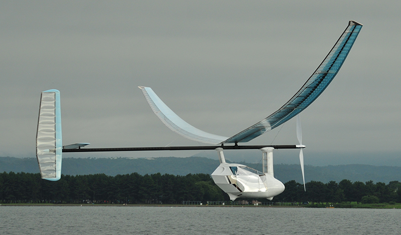
Figure 1: Human-powered aircraft in flight.

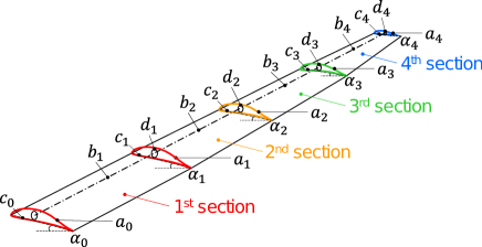
Figure 2: Variables defining the main wing shape.

The variables defining the main wing shape are based on dividing the right wing into $n$ segments, defined by $(n+1)$ cross-sections, as shown in Fig. 2 for the case where $n=4$. The variables include $a_{i}$ for airfoil choice, $b_{i}$ for the length of each segment, $c_{i}$ for the chord length, $\alpha_{i}$ for the angle of attack, and $d_{i}$ for the diameter of the CFRP pipe forming the main spar. These variables are real-valued. Within each segment, the airfoil, chord length, and angle of attack have a distribution based on linear interpolation of values at both cross-sections. The diameter of the CFRP pipe is uniform and defined by $d_{i}$. The airfoil $a_{i}\in[0,3]$ corresponds to well-known HPA airfoils named DAE11, DAE21, DAE31, and DAE41 when taking integer values ${0,1,2,3}$, respectively. For non-integer values, the performance parameters (lift-curve slope, zero-lift angle, drag coefficient, and thickness ratio) are linearly interpolated between $\lfloor a_{i}\rfloor$ and $\lceil a_{i}\rceil$. This interpolation is also applied within each segment.

Variables related to the stacking sequence of the CFRP pipe forming the main spar for segment $i$ are defined by Fig. 3. The CFRP pipe is manufactured by laminating sheets of material called prepregs, which consist of carbon fibers aligned in a specific direction, at angles (orientation angles) that match the expected loads. The CFRP pipe of diameter $d_{i}$ for segment $i$ consists of fixed 4 full-circumference laminates and variable $m$ flange laminates. $m$ varies depending on the optimization problem while Fig. 3 shows an example configuration for $m=4$. In the cross-sectional view, the black area represents the full-circumference laminates, while the red, green, orange, and blue areas represent the flange laminates. The stacking sequence of the CFRP pipe includes three layers of full-circumference laminates with orientation angles of $90\mathrm{°}$/$+45\mathrm{°}$/$-45\mathrm{°}$, $m$ layers of flange laminates with an orientation angle of $0\mathrm{°}$, and one layer of full-circumference laminate with an orientation angle of $90\mathrm{°}$. The wing span direction corresponds to an orientation angle of $0\mathrm{°}$, and the circumferential direction corresponds to an orientation angle of $90\mathrm{°}$. However, for the segment $\lfloor n/2\rfloor+1$, $+45\mathrm{°}$/$-45\mathrm{°}$ is replaced with $+30\mathrm{°}$/$-30\mathrm{°}$. The variables related to the stacking sequence include the starting and ending points $s_{i,j}$ and $e_{i,j}$, and the width $w_{i,j}$ for each of the $j\in{1,\cdots,m}$ flange laminates. $s_{i,j}$ and $e_{i,j}$ are non-dimensional position on the spanwise coordinate where the $(i-1)$ and $i$-th cross-sections are defined as 0 and 1, respectively. Note that for manufacturing reasons, $s_{i,j}\leq s_{i,j+1}$, $e_{i,j}\geq e_{i,j+1}$, and $w_{i,j}<w_{i,j+1}$. These constraints are automatically satisfied based on the definition of the design variables.

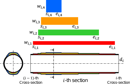
Figure 3: Variables defining the stacking sequence of CFRP pipes.

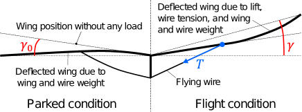
Figure 4: Relationship between wing deflection at parked and flight conditions, dihedral angle, and tension force of the flying wire.

Other variables include the dihedral angle at the wing root $\gamma_{0}$, the tension force $T$ of the flying wire, and the payload $W_{p}$. Fig. 4 illustrates the deflection curve of the main wing when viewed from the front at both parked and flight conditions. By varying $\gamma_{0}$, it is possible to adjust the dihedral angle at the wingtip $\gamma$ during flight, considering the need to provide clearance between the wing and the ground at the parked condition. The flying wire is introduced to relieve some of the bending moment due to lift during flight, thus reducing the weight of the inner CFRP pipes compared to when no flying wire is used. Payload $W_{p}$ represents the mass of cargo or passengers carried by the HPA. These three variables are included as variables in some problems.

III-B Design Variables

The design variables ${\bf x}$ for the benchmark problem change with the level of difficulty in the problem. Therefore, we denote the design variables at three difficulty levels as ${\bf x}_{l}$ for $l\in\{0,1,2\}$. By applying different variable transformations to ${\bf x}_{l}$ based on the level of difficulty, we obtain the variables for defining wing design described in the previous subsection.

III-B1 Difficulty Level $l=0$

In this case, the design variables include segment lengths $b_{i}$, chord lengths $c_{i}$, an angle of attack at wing root $\alpha_{0}$, washout angles $\dot{\alpha_{i}}$, a dihedral angle at wing root $\gamma_{0}$, wire tension $T$, payload $W_{p}$, and the reduction coefficients for reference strains at flight and parked conditions, $r_{0}$ and $r_{1}\in(0,1]$. Note that depending on the problem, $\gamma_{0}$, $T$, and $W_{p}$ may be treated as constants. For $l=0$, airfoil $a_{i}$ is considered a constant, and the diameter of the CFRP pipe $d_{i}$ is defined as $d_{i}=\min_{\tilde{y_{i}}}t(\tilde{y_{i}})c(\tilde{y_{i}})$, where $t(\tilde{y_{i}})$ and $c(\tilde{y_{i}})$ are functions that linearly interpolate wing thickness and chord length in the wing span direction within the $i$th segment using $\tilde{y_{i}}\in[0,1]$ as the non-dimensional spanwise coordinate.

The angle of attack $\alpha_{i}$ at each cross-section is transformed from $\alpha_{0}$ and $\dot{\alpha_{i}}$ as follows:

$$\alpha_{i}=\alpha_{0}+\sum_{i^{\prime}=1}^{i}\dot{\alpha_{i^{\prime}}}$$ (1)

The variables $s_{i,j}$, $e_{i,j}$, and $w_{i,j}$ for each segment are greedily optimized to satisfy constraint $g_{1,i}^{\prime}(\tilde{y_{i}},{\bf x}_{l})<0$ with the use of $r_{0}$ and $r_{1}$:

$$g_{1,i}^{\prime}(\tilde{y_{i}},{\bf x}_{l})=\frac{n_{m}n_{s}}{\epsilon_{u}}\max\left[\frac{\epsilon_{0}(\tilde{y_{i}},{\bf x}_{l})}{r_{0}},\frac{\epsilon_{1}(\tilde{y_{i}},{\bf x}_{l})}{r_{1}}\right]-1$$ (2)

where, $n_{m}=1.5$, $n_{s}=2$, and $\epsilon_{u}=0.0027$ are constants representing load factor, safety factor, and reference strain. $\epsilon_{0}(\tilde{y_{i}},{\bf x}_{l})$ and $\epsilon_{1}(\tilde{y_{i}},{\bf x}_{l})$ are absolute values of compressive strains on the outer surface of CFRP pipe at $\tilde{y_{i}}$ at flight and stationary conditions, respectively.

The flange laminates are optimized using Algorithm 1. $\Delta w$ represents the minimum increment of the laminate width, set to 2 [mm] in this paper for manufacturing convenience. By applying Algorithm 1 in order from the main spar near the wingtip ($i=n$), $s_{i,j}$, $e_{i,j}$, and $w_{i,j}$ are determined to satisfy the strength constraint. To ensure that the design space for $l=0,1$ is included in that for $l=2$, lines 17-26 in Algorithm 1 is applied to align one end of each laminate with the section boundary (pipe end). Smaller values of $r_{0}$ and $r_{1}$ increase the stiffness of the main spar and make it easier to find solutions that satisfy deflection constraints.

Algorithm 1 Flange laminate optimization

0:  $i,\ m,\ r_{0},\ r_{1},\ \Delta w,\ {\bf x}_{l}$

0:  $s_{i,j},\ e_{i,j},\ w_{i,j}\ (j=1,2,\cdots,m)$

1:  Initialize $i$-th beam: $s_{i,j}=0,\ e_{i,j}=1,\ w_{i,1}=\pi d_{i}/12,\ w_{i,j+1}=w_{i,j}+\Delta w,\ \Delta\phi=0$

2:  Evaluate $g_{1,i}^{\prime}(\tilde{y_{i}},{\bf x}_{l})$

3:  while $\exists\tilde{y_{i}}\in[0,1],\ g_{1,i}^{\prime}(\tilde{y_{i}},{\bf x}_{l})>0$ do

4:     $\Delta\phi\leftarrow\Delta\phi+\pi/180$

5:     $w_{i,1}=\left(\pi/6+\Delta\phi\right)d_{i}/2,\ w_{i,j+1}=w_{i,j}+\Delta w$

6:     Evaluate $g_{1,i}^{\prime}(\tilde{y_{i}},{\bf x}_{l})$

7:  end while

8:  for $j=m:1$ do

9:     Evaluate $g_{1,i}^{\prime}(\tilde{y_{i}},{\bf x}_{l})$ with $e_{i,j}=0$

10:     $s_{i,j}=\min(\tilde{y_{i}}\in[0,1]\mid g_{1,i}^{\prime}(\tilde{y_{i}},{\bf x}_{l})>0)$

11:     $e_{i,j}=\max(\tilde{y_{i}}\in[0,1]\mid g_{1,i}^{\prime}(\tilde{y_{i}},{\bf x}_{l})>0)$

12:     if $j<m$ then

13:        $s_{i,j}\leftarrow\min(s_{i,j},s_{i,j+1})$

14:        $e_{i,j}\leftarrow\max(e_{i,j},e_{i,j+1})$

15:     end if

16:  end for

17:  $S_{i}=\sum_{j=1}^{m}s_{i,j}$, $E_{i}=\sum_{j=1}^{m}(1-e_{i,j})$

18:  if $S_{i}E_{i}>0$ then

19:     for $j=m:1$ do

20:        if $S_{i}>E_{i}$ then

21:           $e_{i,j}=1$

22:        else

23:           $s_{i,j}=0$

24:        end if

25:     end for

26:  end if

III-B2 Difficulty Level $l=1$

In addition to the design variables from level $l=0$, airfoil $a_{i}$ and the diameter reduction factor $\tilde{d_{i}}\in(0,1]$ for the CFRP pipe are included as design variables for level $l=1$. The diameter of the CFRP pipe is defined as $d_{i}=\tilde{d_{i}}\min_{\tilde{y_{i}}}t(\tilde{y_{i}})c(\tilde{y_{i}})$. The flange laminates $s_{i,j}$, $e_{i,j}$, and $w_{i,j}$ are optimized in the same way as for level $l=0$ using Algorithm 1. However, the reduction factors $r_{0,i}$ and $r_{1,i}$ for each segment vary, and they are used as design variables instead of $r_{0}$ and $r_{1}$.

III-B3 Difficulty Level $l=2$

In level $l=2$, flange laminates $s_{i,j}$, $e_{i,j}$, and $w_{i,j}$ are determined with different way from level $l=1$. The design variables consist of the change in length and width between each layer of flange laminate $\dot{l}_{i,j}$ and $\dot{w}_{i,j}$ and the spanwise reference position $\xi_{i}\in[0,1]$. The flange laminate is defined using the following equations:

$$l_{i,j}=\max\left(0,\;1-\sum_{j^{\prime}=1}^{j}\dot{l}_{i,j^{\prime}}\right)$$ (3)

$$\tilde{\xi_{i}}=\text{round}\left(\frac{1}{1+\exp(-50(\xi_{i}-0.5))},\;4\right)$$ (4)

$$s_{i,j}=\tilde{\xi_{i}}(1-l_{i,j})$$ (5)

$$e_{i,j}=\tilde{\xi_{i}}+l_{i,j}(1-\tilde{\xi_{i}})$$ (6)

$$w_{i,j}=\frac{\pi d_{i}}{12}-\Delta w+\sum_{j^{\prime}=1}^{j}\dot{w}_{i,j^{\prime}}$$ (7)

Equation 4 uses a sigmoid function and rounding to convert $\xi_{i}$ to $\tilde{\xi_{i}}$, which improves the probability that each laminate connects to one end of the CFRP pipe and leads to a reasonable design.

III-C Objective Functions and Constraints

Each benchmark problem is constructed by selecting a subset of the fundamental 11 objective functions, $f_{i}$, and 5 constraint conditions, $g_{i}\leq 0$, as shown in Table I. The functions $P$, $D$, $V$, $\Phi$, $E$, $W_{0}$, and $B$ represent the required power, drag, cruise speed, twist angle at wingtip, wing efficiency, empty weight, and wing span, respectively. The variables $\delta$ and $\delta_{park}$ denote the wingtip displacement (positive upwards) at flight and parked conditions, relative to the wing root height. $\epsilon_{max}$ represents the maximum strain in CFRP pipes at both parked and flight conditions, and $\gamma$ represents the dihedral angle at wingtip at the flight condition. Additionally, $\eta=0.85\times 0.95$ is the product of propeller and drivetrain efficiency, $\gamma_{u}=$$$ is maximum dihedral angle, $P_{max}=400$ [W] is maximum required power, and $V_{min}=7.3$ [m/s] is the minimum cruise speed. Since $V$, $E$, and $W_{p}$ are functions to be maximized, a negative sign is applied to $f_{3}$, $f_{6}$, and $f_{11}$ to convert them into minimization problems.

TABLE I: Fundamental functions and penalty weights for unconstrained problmes.

Function	Unit	Weight
$f_{1}=P({\bf x}_{l})=D({\bf x}_{l})V({\bf x}_{l})/\eta$	W	$v_{1}=10$
$f_{2}=D({\bf x}_{l})$	N	$v_{2}=1$
$f_{3}=-V({\bf x}_{l})$	m/s	$v_{3}=1$
$f_{4}=\max(|\delta({\bf x}_{l})|,|\delta_{park}({\bf x}_{l})|)$	m	$v_{4}=0.5$
$f_{5}=\Phi({\bf x}_{l})$	deg	$v_{5}=0.1$
$f_{6}=-E({\bf x}_{l})$	-	$v_{6}=0.1$
$f_{7}=W_{0}({\bf x}_{l})$	kg	$v_{7}=1$
$f_{8}=B=2\sum_{i=1}^{n}b_{i}$	m	$v_{8}=1$
$f_{9}=\alpha_{0}$	deg	$v_{9}=1$
$f_{10}=T$	N	$v_{10}=200$
$f_{11}=-W_{p}$	kg	$v_{11}=10$
$g_{1}=n_{m}n_{s}\epsilon_{max}({\bf x}_{l})/\epsilon_{u}-1$	-	$w_{1}=10$
$g_{2}=B(\sin{\gamma({\bf x}_{l})}-\sin{\gamma_{u}})/2$	m	$w_{2}=2$
$g_{3}=-\delta_{park}({\bf x}_{l})$	m	$w_{3}=2$
$g_{4}=P({\bf x}_{l})-P_{max}$	W	$w_{4}=0.1$
$g_{5}=1-(V({\bf x}_{l})/V_{min})^{3}$	-	$w_{5}=10$

Many of the objective functions and constraints are functions of most elements in ${\bf x}_{l}$. However, the wing efficiency $E$ for $f_{6}$ depends only on the variables related to the wing shape: airfoil $a_{i}$, section length $b_{i}$, chord length $c_{i}$, and angle of attack $\alpha_{i}$. $f_{8}$ is the sum of $b_{i}$, while $f_{9}$ through $f_{11}$ are specific design variables themselves. Additionally, functions that have the dihedral angle at wing root $\gamma_{0}$ as a variable are limited to $f_{4}$, $g_{2}$, and $g_{3}$, and only functions $f_{4}$ and $g_{2}$ have all elements in ${\bf x}_{l}$ as variables.

The objective functions and constraints are evaluated by solving integral equations based on lifting line theory and differential equations for deflection based on beam-column theory. Computational grids with $N_{aero}=50$ and $N_{struc}=301$ points are used for solving these equations, respectively.

III-D Definition of Each Problem

By selecting a subset of functions from Table I, we define 3 single-objective problems and 17 multi-objective problems. Each problem has three levels of difficulty, resulting in a total of 60 benchmark problems. The benchmark problems proposed in this paper are denoted as HPA$MNL$-$l$, where $M$ is the number of objective functions, $N$ is the number of inequality constraints (excluding box constraints), $L$ is the problem ID, and $l$ is the difficulty level, which may be omitted if irrelevant. The wing segmentation number $n$ is a parameter that increases or decreases the problem dimension, and in this paper, we set $n=4$. $n$ should be an even number to obtain a realistic design.

TABLE II: Objective Functions, Constraints, Design Variables, and Problem Dimension in $n=4$.

Problem

$f_{1}$

$f_{2}$

$f_{3}$

$f_{4}$

$f_{5}$

$f_{6}$

$f_{7}$

$f_{8}$

$f_{9}$

$f_{10}$

$f_{11}$

$g_{1}$

$g_{2}$

$g_{3}$

$g_{4}$

$g_{5}$

$\gamma_{0}$

$T$

$W_{p}$

$m$

$|{\bf x}_{0}|$

$|{\bf x}_{1}|$

$|{\bf x}_{2}|$

HPA131, 101

✓

✓

✓

✓

✓

10

17

32

108

HPA142, 102

✓

✓

✓

20

16

31

187

HPA143, 103

✓

✓

✓

✓

✓

✓

✓

20

18

33

189

HPA241, 201

✓

✓

✓

✓

✓

✓

✓

✓

10

18

33

109

HPA222, 202

✓

✓

✓

✓

20

16

31

187

HPA233, 203

✓

✓

✓

✓

✓

✓

✓

✓

20

19

34

190

HPA244, 204

✓

✓

✓

✓

✓

✓

✓

✓

20

18

33

189

HPA245, 205

✓

✓

✓

✓

✓

✓

✓

✓

20

18

33

189

HPA341, 301

✓

✓

✓

✓

✓

✓

✓

✓

✓

10

18

33

109

HPA322, 302

✓

✓

✓

✓

✓

20

16

31

187

HPA333, 303

✓

✓

✓

✓

✓

✓

✓

✓

✓

20

19

34

190

HPA344, 304

✓

✓

✓

✓

✓

✓

✓

✓

✓

20

18

33

189

HPA345, 305

✓

✓

✓

✓

✓

✓

✓

✓

✓

20

18

33

189

HPA441, 401

✓

✓

✓

✓

✓

✓

✓

✓

✓

✓

20

18

33

189

HPA422, 402

✓

✓

✓

✓

✓

✓

20

16

31

187

HPA443, 403

✓

✓

✓

✓

✓

✓

✓

✓

✓

✓

20

18

33

189

HPA541, 501

✓

✓

✓

✓

✓

✓

✓

✓

✓

✓

✓

20

18

33

189

HPA542, 502

✓

✓

✓

✓

✓

✓

✓

✓

✓

✓

✓

✓

20

19

34

190

HPA641, 601

✓

✓

✓

✓

✓

✓

✓

✓

✓

✓

✓

✓

20

18

33

189

HPA941, 901

✓

✓

✓

✓

✓

✓

✓

✓

✓

✓

✓

✓

✓

✓

✓

✓

20

19

34

190

In Table II, we present the objective functions, constraints, and the design variables used for each problem, as well as the maximum number of layers in CFRP flange laminates, $m$, and the dimension of design variables $|{\bf x}_{l}|$ when $n=4$ for each difficulty level. The dimension of the design variables varies with $n$, $m$, and $k$ as follows: $|{\bf x}_{0}|=3n+4+k$, $|{\bf x}_{1}|=7n+3+k$, and $|{\bf x}_{2}|=(2m+6)n+3+k$, where $k$ is the number of variables used among $\gamma_{0}$, $T$, and $W_{p}$ listed in Table II. In unconstrained problems with $N=0$, we modify the objective functions $f_{i}$ as $f_{i}^{\prime}$ using the penalty coefficients $v_{i}$ and $w_{j}$ from Table I as:

$$f_{i}^{\prime}=f_{i}+\max\left(0,\;v_{i}\sum_{j\in\mathcal{G}}w_{j}g_{j}\right)$$ (8)

where, $\mathcal{G}\subset\{1,2,3,4,5\}$ is a set composed of constraint numbers used in each problems from Table II.

IV Numerical Experiment

IV-A Setups

We conducted experiments on a total of 60 unconstained HPA problems with Eq. 8 as objective functions because most widely available evolutionary algorithms and Bayesian optimization methods lack sufficient support for handling constraints. The lower and upper bounds of the design variables are shown in Table III where $g$ [m/s] is the gravitational acceleration, while all design variables have been normalized to the range [0,1] in the implementation.

IV-A1 Single-Objective Problems

We employed algorithms from the black-box optimization libraries pymoo[12], BoTorch[13], and Optuna™[14]. From pymoo, we utilized four evolutionary algorithms, namely covariance matrix adaptation evolution strategy (CMA-ES)[15], particle swarm optimization (PSO), differential evolution (DE), and genetic algorithm (GA), with default settings for parameters except for the population size. From BoTorch, we utilized Bayesian optimization methods, namely Gaussian process regression (GPR) with q-expected improvement (GP-qEI) [16], and trust region Bayesian optimization (TuRBO)[17]. Optuna™provided the tree-structured Parzen estimator (TPE)[18].

In all algorithms, the population size and the number of initial sample points were set to 20, the maximum function evaluation was set to 1,000, the number of independent runs was set to 11. The batch size (number of additional sample points at each iteration) of GP-qEI and TuRBO was set to 5 to reduce the computational cost for GPR. In TPE, one sample point was added in each iteration. Other parameters were set to the default values in each library.

IV-A2 Multi-Objective Problems

For multi-objective HPA problems, we employed six algorithms for pymoo: non-dominated sorting genetic algorithm II (NSGA-II) [19] and III (NSGA-III) [20], multi-objective evolutionary algorithm based on decomposition (MOEA/D) [21], S-metric selection evolutionary multi-objective optimisation algorithm (SMS-EMOA) [22], reference vector guided evolutionary algorithm (RVEA) [23], and adaptive geometry estimation based many-objective Evolutionary algorithm II (AGE-MOEA-II) [24]. In all algorithms, the population size was set to $40M$, where $M$ is the number of objective functions, and the maximum function evaluation was set to 72,000 for problems with $l=0,1$, and 216,000 for problems with $l=2$. Reference vectors for NSGA-III, MOEA/D, RVEA are generated by the Riesz s-Energy method [25] implemented in pymoo, and the number of vectors is the same as the population size. As pointed out by He et al. [26], objective function normalization was employed for MOEA/D, SMS-EMOA, and RVEA to improve their performance. The normalization method was the same as that implemented for SMS-EMOA in pymoo. Other parameters were set to the default values in pymoo.

We conducted 11 independent runs and calculated the $\text{IGD}^{+}$ for the normalized objective functions. The reference points for $\text{IGD}^{+}$ were selected from non-dominated solutions (NDSs) obtained by hot-started above six algorithms where initial population consists of NDSs from all cold-started runs across problems and difficulty levels. The normalization of the objective functions also used the Utopia and Nadir points from the reference points of $\text{IGD}^{+}$.

TABLE III: Upper and Lower Bounds for Design Variables.

$l$	${\bf x}_{l}$	Dimension	Min.	Max.	Unit
0,1,2	$b_{i}$	$n$	$8/n$	$20/n$	m
	$c_{i}$	$n+1$	0.4	1.5	m
	$\alpha_{0}$	1	4	7	deg
	$\dot{\alpha_{i}}$	$n$	$-8/n$	0	deg
	$\gamma_{0}$	1	0	4	deg
	$T$	1	0	$135g$	N
	$W_{p}$	1	0	60	kg
1,2	$a_{i}$	$n+1$	0	3	-
	$\tilde{d_{i}}$	$n$	0.8	1	-
0	$r_{0}$	1	0.01	1	-
	$r_{1}$	1	0.01	1	-
1	$r_{0,i}$	$n$	0.01	1	-
	$r_{1,i}$	$n$	0.01	1	-
2	$\dot{l}_{i,j}$	$mn$	0	1	-
	$\dot{w}_{i,j}$	$mn$	0.002	0.26	m
	$\xi_{i}$	$n$	0	1	-

IV-B Pareto Front Shapes

The $\text{IGD}^{+}$ reference points for two-objective and three-objective problems are shown in Fig. 6. While many problems have convex PF, HPA203 and 303 have linear PF and HPA205 and 305 have concave PF in particular cross-sections. When HPA305 is sliced parallel to the $f_{10}$ axis, a PF shape similar to HPA205 appears. HPA304 forms an inverted triangular PF. In HPA302, there is a strong positive correlation between $f_{4}$ and $f_{5}$, causing a partially degenerated PF near the minimum values of these objectives. In HPA problems, the PFs of higher-difficulty level dominate those of lower-difficulty level since the design space of higher-difficulty level includes that of lower-difficulty levels.

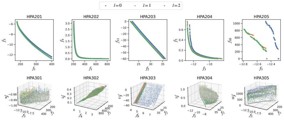
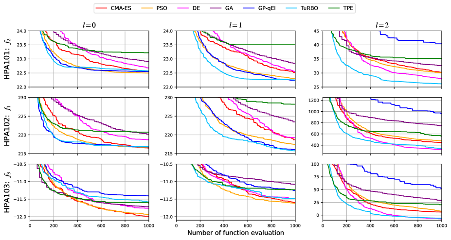
Figure 5: Pareto Front Shapes with Reference Points for $\text{IGD}^{+}$ in Each Difficulty Level.

Figure 6: Histories of objective function values.

IV-C Results

IV-C1 Single-Objective Problems

For each algorithm, Fig. 6 presents the averaged results over 11 runs of the best objective function values at each point up to 1,000 function evaluations. It should be noted that while the vertical axes for $l=0,1$ are the same for each problem, the axis for $l=2$ differs.

In HPA101-0,1 and HPA102-0,1, algorithms such as TuRBO, GP-qEI, and PSO demonstrated consistently high performance across a broad range. These algorithms are widely utilized in computationally expensive problems [27, 28], typically involving a maximum of 100 to 1,000 function evaluations. This suggests similarities between these benchmark problems and real-world problems. The effective application of algorithms incorporating GPR indicates that HPA problems likely exhibit moderate multimodality, as intended. Conversely, HPA103-0,1 exhibited distinct characteristics compared to HPA101-0,1 and HPA102-0,1, with PSO, CMA-ES, and DE achieving favorable outcomes, while GP-qEI and TuRBO showed only moderate success. This suggests that these problems might pose challenges for surrogate model approximation.

For problems at difficulty level $l=2$, TuRBO, specifically designed for high-dimensional problems, generally outperformed others, with DE and CMA-ES following. In contrast, GP-qEI exhibited poorer performance due to the high dimensionality. Interestingly, TPE demonstrated performance comparable to TuRBO up to the 100th function evaluation.

Additionally, the design space of problems at difficulty level $l=1$ includes that of $l=0$, and similarly, $l=2$ includes the space of $l=1$. However, the results obtained suggest that in some instances, lower difficulty levels $l$ might yield superior outcomes. This implies that simplifying problems, particularly when the number of evaluations is limited, could be an effective strategy for attaining better solutions in real-world problemss.

IV-C2 Multi-Objective Problems

Table IV presents the mean $\text{IGD}^{+}$ in 11 runs for each algorithm. AGE-MOEA-II achieves the smallest $\text{IGD}^{+}$ across 17 problems, including 14 many-objective problems. NAGA-II (smallest $\text{IGD}^{+}$ across 13 problems) and SMS-EMOA (smallest $\text{IGD}^{+}$ across 11 problems) exhibit superior performance in two and three-objective problems, respectively. To evaluate the overall performance of the algorithms, we computed a geometric mean of mean $\text{IGD}^{+}$ in Table IV. AGE-MOEA-II, SMS-EMOA, and NSGA-II show the best three geometric mean of $\text{IGD}^{+}$. On the other hand, MOEA/D exhibits the largest $\text{IGD}^{+}$ in most problems although objective function normalization was employed. RVEA also shows modest performance while it achieves the smallest $\text{IGD}^{+}$ in across 5 problems.

In each problem, the $\text{IGD}^{+}$ values for $l=2$ are significantly higher than for $l=1$. Despite both $l=1$ and $l=2$ problems having nearly identical PFs, as shown in Fig. 6, it suggests that the six algorithms did not obtain well-converged and diverse NDSs for the $l=2$ problems due to their high dimensionality. Fig. 7 shows NDSs obtained by NSGA-II at the median $\text{IGD}^{+}$ runs in the two-objective problems for each difficulty level. Both convergence and diversity are not sufficient for the $l=2$ problems.

Additionally, HPA204 and 205 are hard to optimize even for $l=0,1$ especially near the extreme solution for $f_{3}$ because solutions around $f_{3}$ minimum have different features in design variables from those around the other side. Such solutions were easily obtained by extending the number of objective functions from HPA204 to HPA304 and from HPA205 to HPA305. Fig. 8 shows NDSs for HPA204 and 205 obtained by SMSEMOA at the median $\text{IGD}^{+}$ runs in HPA304 and 305, respectively. Solving two-objective problems as if they were three-objective problems, similar to the approach of transforming a single-objective problem into a multi-objective one as discussed in [29], improves the diversity of NDSs as compared to the case shown in Fig. 7.

Table IV also includes the mean evaluation time of objective functions when generating 1,000 random solutions for each problem. The CPU used for calculations was the AMD Ryzen 5 3400G 3.70GHz. In all problems, the evaluation time per solution is within 0.15 seconds, and 10,000 solutions can be evaluated within 25 minutes. For problems with $l=0$ and $l=1$, where multiple strength evaluations are performed during the flange laminate optimization with Algorithm 1, the evaluation time is approximately three times longer than that of $l=2$ problems.

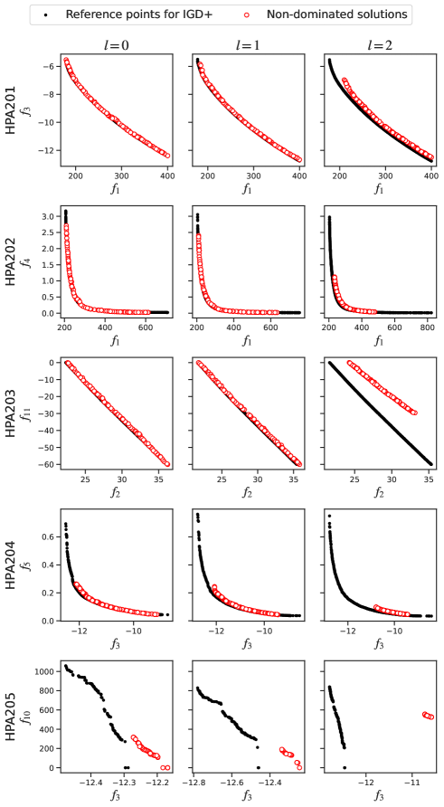
Figure 7: Non-dominated solutions obtained by NSGA-II at the median $\text{IGD}^{+}$ runs in the two-objective problems.

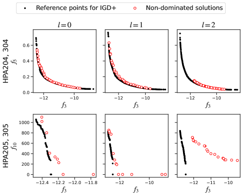
Figure 8: Non-dominated solutions obtained by SMSEMOA at the median $\text{IGD}^{+}$ runs in HPA304 and 305, projected into corresponding two-objective problems.

TABLE IV: Mean $\text{IGD}^{+}$ and mean evaluation time per solution. The background colors indicate the relative magnitudes of $\text{IGD}^{+}$ for each problem, with the smallest $\text{IGD}^{+}$ in each problem highlighted in bold.

V Summary

We proposed a set of single and multi-objective optimization benchmark problems focusing on human-powered aircraft design. Each problem can be adjusted in difficulty across three levels by modifying the definition of design variables, and the dimension of design variables can be further increased or decreased through a wing segmentation parameter. In multi-objective problems, their Pareto fronts exhibit diverse shapes, including the inverted triangle frequently observed in real-world problems, as well as convex, linear, concave, and partially degenerated forms. By applying representative evolutionary algorithms and Bayesian optimization methods to these benchmark problems, we confirmed that they likely exhibit moderate multimodality of engineering design problems and existing algorithms rarely yield well-converged and diverse non-dominated solutions in the high-difficulty level.

References

- [1] X. Li, K. Tang, M.N. Omidvar, Z. Yang, K. Qin, and H. China, “Benchmark functions for the CEC 2013 special session and competition on large-scale global optimization,” echnical Report, Evolutionary Computation and Machine Learning Group, RMIT University, 2013.
- [2] E. Zitzler, K. Deb, and L. Thiele, “Comparison of multiobjective evolutionary algorithms: empirical results,” Evol. Comput., vol. 8, no. 2, pp. 173–195, 2000.
- [3] K. Deb, L. Thiele, M. Laumanns, E. Zitzler, “Scalable test problems for evolutionary multiobjective optimization,” Evolutionary Multiobjective Optimization, pp. 105–145, 2005.
- [4] H. Ishibuchi, Y. Setoguchi, H. Masuda, and Y. Nojima, “Performance of Decomposition-Based Many-Objective Algorithms Strongly Depends on Pareto Front Shapes,” IEEE Trans. Evol. Comput., vol. 21, no. 2, pp. 169–190, 2017.
- [5] H. Ishibuchi, L. He, and K. Shang, “Regular Pareto Front Shape is not Realistic,” Proc. IEEE Congr. Evol. Comput., pp. 2034–2041, 2019.
- [6] N. Hamada, “Simple Problems: the Simplicial Gluing Structure of Pareto Sets and Pareto Fronts,” Proc. Genetic Evol. Comput. Conf., pp. 315–316, 2017.
- [7] R. Tanabe and H. Ishibuchi, “An easy-to-use real-world multi-objective optimization problem suite,” Appl. Soft Comput., vol. 89, pp. 106078, 2020.
- [8] Z. Wang, C. Gehring, P. Kohli, and S. Jegelka, “Batched large-scale Bayesian optimization in high-dimensional spaces,” Proc. Int. Conf. Artificial Intelligence and Statistics, pp. 745–754, 2018.
- [9] S.J. Daniels, A.AM Rahat, R.M. Everson, G.R. Tabor, and J.E. Fieldsend, “A suite of computationally expensive shape optimisation problems using computational fluid dynamics,” Proc. Int. Conf. Parallel Problem Solving from Nature, pp. 745–754, 2018.
- [10] V. Volz, B. Naujoks, P. Kerschke, and T. Tušar, “Single-and multi-objective game-benchmark for evolutionary algorithms,” Proc. Genetic Evol. Comput. Conf, pp. 647–655, 2019.
- [11] C. He, Y. Tian, H. Wang, and Y. Jin, “A repository of real-world datasets for data-driven evolutionary multiobjective optimization,” Complex Intell. Syst., vol. 6, pp. 189–197, 2020.
- [12] J. Blank and K. Deb, “Pymoo: multi-objective optimization in python,” IEEE Access, vol. 8, pp. 89497–89509, 2020.
- [13] M. Balandat, B. Karrer, D. Jiang, S. Daulton, B. Letham, A.G. Wilson, and E. Bakshy, “BoTorch: a framework for efficient Monte-Carlo Bayesian optimization,” Proc. Advances in Neural Information Processing Systems, vol. 33, pp. 21524–21538, 2020.
- [14] T. Akiba, S. Sano, T. Yanase, T. Ohta, and M. Koyama, “Optuna: a next-generation hyperparameter optimization framework,” Proc. ACM SIGKDD Int. Conf. Knowledge Discovery & Data Mining, pp. 2623–2631, 2019.
- [15] N. Hansen and A. Ostermeier, “Completely derandomized self-adaptation in evolution strategies,” Evol. Comput., vol. 9, no. 2, pp. 159–195, 2001.
- [16] J.T. Wilson, R. Moriconi, F. Hutter, and M.P. Deisenroth, “The reparameterization trick for acquisition functions,” arXiv preprint arXiv:1712.00424, 2017.
- [17] D. Eriksson, M. Pearce, J. Gardner, R.D. Turner, and M. Poloczek, “Scalable global optimization via local Bayesian optimization,” Proc. Advances in Neural Information Processing Systems, vol. 32, 2019.
- [18] J. Bergstra, R. Bardenet, Y. Bengio and B. Kégl, “Algorithms for hyper-parameter optimization,” Proc. Advances in Neural Information Processing Systems, vol. 24, 2011.
- [19] K. Deb, A. Pratap, S. Agarwal, and T. Meyarivan, “A fast and elitist multiobjective genetic algorithm: NSGA-II,” IEEE Trans. Evol. Comput., vol. 6, no. 2, pp. 182–197, 2002.
- [20] K. Deb and H. Jain, “An evolutionary many-objective optimization algorithm using reference-point—based nondominated sorting approach, part I: solving problems with box constraints,” IEEE Trans. Evol. Comput., vol. 18, no. 4, pp. 577–601, 2014.
- [21] Q. Zhang and H. Li, “MOEA/D: a multiobjective evolutionary algorithm based on decomposition,” IEEE Trans. Evol. Comput., vol. 11, no. 6, pp. 712–731, 2007.
- [22] N. Beume, B. Naujoks, and M. Emmerich, “SMS-EMOA: multiobjective selection based on dominated hypervolume,” Eur. J. Oper. Res., vol. 181, no. 3, pp. 1653–1669, 2007.
- [23] R. Cheng, Y. Jin, M. Olhofer, and B. Sendhoff, “A reference vector guided evolutionary algorithm for many-objective optimization,” IEEE Trans. Evol. Comput., vol. 20, no. 5, pp. 773–791, 2016.
- [24] A. Panichella, “An improved Pareto front modeling algorithm for large-scale many-objective optimization,” Proc. Genetic Evol. Comput. Conf., pp. 565–573, 2022.
- [25] D.P. Hardin and E.B. Saff, “Minimal Riesz energy point configurations for rectifiable d-dimensional manifolds,” Adv.Math., vol. 193, no. 1, pp. 174-204, 2005.
- [26] L. He, Y. Nan H. Ishibuchi, and D. Srinivasan, “Effects of Objective Space Normalization in Multi-Objective Evolutionary Algorithms on Real-World Problems,” Proc. Genetic Evol. Comput. Conf, pp. 670–678, 2023.
- [27] N. Namura, K. Shimoyama, S. Obayashi, Y. Ito, S. Koike, and K. Nakakita, “Multipoint design optimization of vortex generators on transonic swept wings,” J. Aircraft., vol. 56, no. 4, pp. 1291–1302, 2019.
- [28] C. Sun and Y. Jin, R. Cheng, J. Ding, and J. Zeng, “Surrogate-assisted cooperative swarm optimization of high-dimensional expensive problems,” IEEE Trans. Evol. Comput., vol. 21, no. 4, pp. 644–660, 2017.
- [29] J.D. Knowles, R.A. Watson, and D.W. Corne, “Reducing local optima in single-objective problems by multi-objectivization,” in Proc. Int. Conf. Evol. Multi-Criterion Optim., pp. 269–283, 2001.