Revisiting RXTE observations of MXB 0656–072 during the type I outbursts in 2007–2008

Abstract

We report on the timing characteristics of MXB 0656–072 throughout its 2007–2008 type I outbursts utilising RXTE/PCA and Fermi/GBM data. Using pulse timing technique, we explore the spin frequency evolution of the source during this interval. Subsequently, by examining the torque–luminosity relation, we show that the overall frequency evolution is substantially in line with the Ghosh–Lamb model. Furthermore, the residuals of the spin frequencies do not exhibit clear orbital modulations, which possibly indicate that the system is observed on a relatively top view. In the RXTE/PCA observations, the pulsed emission is found to be disappearing below $\sim$$5\times 10^{36}$ erg s^-1, whereas the profiles maintain stability above this value within our analysis timeframe. In addition, we incorporate two novel methods along with the conventional Deeter method in order to generate higher-resolution power density spectra (PDS). A red noise pattern in the PDSs is also verified in these new methods, common in disk-fed sources, with a steepness of $\Gamma\sim-2$, reaching saturation at a time-scale of $\sim$150 d. Considering the models for spectral transitions, we discuss the possible scenarios for the dipolar magnetic field strength of MXB 0656–072 and its coherence with deductions from the cyclotron resonance scattering feature (CRSF).

1 Introduction

MXB 0656–072 is a transient BeXRB system consisting of a neutron star with a spin period of 160.7 s (Morgan et al., 2003) and a O9.7Ve spectral type donor star (Pakull et al., 2003). Despite being among the earliest transients discovered (Clark et al., 1975), this source still stands as a relatively less explored member. Following its discovery, MXB 0656–072 entered a state of quiescence, only to rebrighten in 2003 during a two-month outburst episode between October and December. Analysis of RXTE data by (McBride et al., 2006b) classified the outburst as type II (see e.g. Reig, 2011, for a review about BeXRBs), revealing a cyclotron resonance scattering feature (CRSF) at $\sim$33 keV, and implying a magnetic field strength of $\sim$$3.7\times 10^{12}$ G. Furthermore, they estimated a distance of 3.9$\pm$0.1 kpc using optical observations. However, the source is reported to be at a distance of 5.7$\pm$0.5 kpc in the Gaia Early Data Release 3 (EDR3) catalogue (Source ID: 3052677318793446016), which is not entirely consistent with the aforementioned value (Gaia Collaboration et al., 2016, 2021).

The second, and the most recent, reappearance of MXB 0656–072 lasted for about one year. The source exhibited a series of X-ray bursts between 2007 November and 2008 November, as observed by INTEGRAL (Kreykenbohm et al., 2007), RXTE (Pottschmidt et al., 2007), Swift (Kennea et al., 2007), and Fermi . During the series of type I outbursts, RXTE/PCA–HEXTE spectra show a CRSF at the luminosity of $\sim$$6.6\times 10^{36}$ erg s^-1 (for 3.9 kpc) in the 3–22 keV energy band (Yan et al., 2012). Through analysis of Swift/BAT and RXTE/ASM data, Yan et al. (2012) deduced an orbital period of $\sim$101.2 d; nevertheless, the specific orbital parameters characterising the system are yet to be established. Their analysis highlighted that the spectra are best described by an absorbed low-energy cut-off power law, accompanied by a CRSF at $\sim$30 keV and an iron line at $\sim$6.4 keV. Furthermore, Nespoli et al. (2012) probed the multiwavelength variability of the transient system MXB 0656–072. In addition to studies on outbursts, MXB 0656–072 is also studied in its quiescence phase using data from Chandra observatory (Tsygankov et al., 2017) and most recently from NuSTAR (Raman et al., 2023).

This paper focuses on the examination of timing and pulse variability of MXB 0656–072 throughout its 2007–2008 outburst. The structure of the paper is as follows: In Section 2, the data and the associated reduction tools used in this study are detailed. Section 3 outlines the methodology and the results of pulse timing and torque-luminosity analysis, followed by a comprehensive investigation of timing noise behaviour of the source in Section 4. Finally, in Section 5, we discuss the physical interpretations of our results within the context of prior research findings.

2 Data

Our study concentrates on the series of type I outbursts of MXB 0656–072 during 2007–2008. The outburst sequence was extensively monitored with RXTE/PCA (Jahoda et al., 1996) across the observation sets P93032 and P93423. The RXTE monitoring campaign, started on 2007 November 14 and ended on 2008 November 18, consists of 172 individual observations. Typical exposures varied between 0.5 and 28 ks throughout these observations.

Analysis of the RXTE/PCA observations are performed using the heasoft v6.31 software. Data filtering included conditions, such as elevation angle higher than 10 degrees, source offset below 0.02%, and electron contamination under 0.1. Additionally, to enhance the signal-to-noise ratio, data collected within 30 minutes of the South Atlantic Anomaly peak were excluded.

Utilising the GoodXenon mode events, we generate a light curve with a 0.125 s time resolution in the 3–20 keV energy band. Since there are different numbers of proportional counter units (PCUs) active during each observation, we use the CORRECTLC command to adjust the count rates to reflect the simultaneous operation of all five PCUs. Finally, the photon arrival times of the light curve are corrected to the barycenter for the timing analysis.

With the aim of measuring the flux level of each observation, we further extract the spectrum for each observation using only PCU2 top layer data in standard2f mode. We used EPOCH 5C model for background generation; and we used the bright background model unless the source count rate drops below <40 cts/s/PCU as suggested by the RXTE team. In the 3–20 keV energy range, each spectrum is modelled with an absorbed power law to measure the unabsorbed flux levels in the given range. We also add a Gaussian line to the model to represent the iron line emission when it is statistically significant. Resulting 3–20 keV flux measurements are then converted to the luminosity, assuming a distance of 5.7 kpc.

3 Pulse Timing and Torque–Luminosity Relation

We start by calculating a nominal spin frequency through folding the barycenter-corrected RXTE/PCA light curve at statistically independent trial frequencies (Leahy et al., 1983). Next, we fold the light curve at the nominal spin period to generate 20-phase-bin pulse profiles for each observation. In cases where the time difference between consecutive observations is less than 1 day, we merge them together and extract a combined pulse profile. To determine the time of arrivals (TOAs) of the pulses, each profile is transformed into a Fourier harmonic representation and cross-correlated (Deeter & Boynton, 1985) with the template profile which is chosen as the one with the highest $\chi^{2}$ among them.

The observed pulsed emission profiles during this interval possess a single-peaked shape. We represent the 3D plot of the normalised pulses sorted by RXTE/PCA count rates in Figure 1. The pulse profiles do not exhibit a significant evolution over either luminosity or time. The only exception is that we cannot observe any pulsed emission in the last few RXTE/PCA observations during which the source luminosity drops below $\sim$$5\times 10^{36}$ erg s^-1. It should be noted that the source emission stays in the order of 10^36-37 erg s^-1 within the data set in our analysis, and the deduced interpretations are made accordingly.

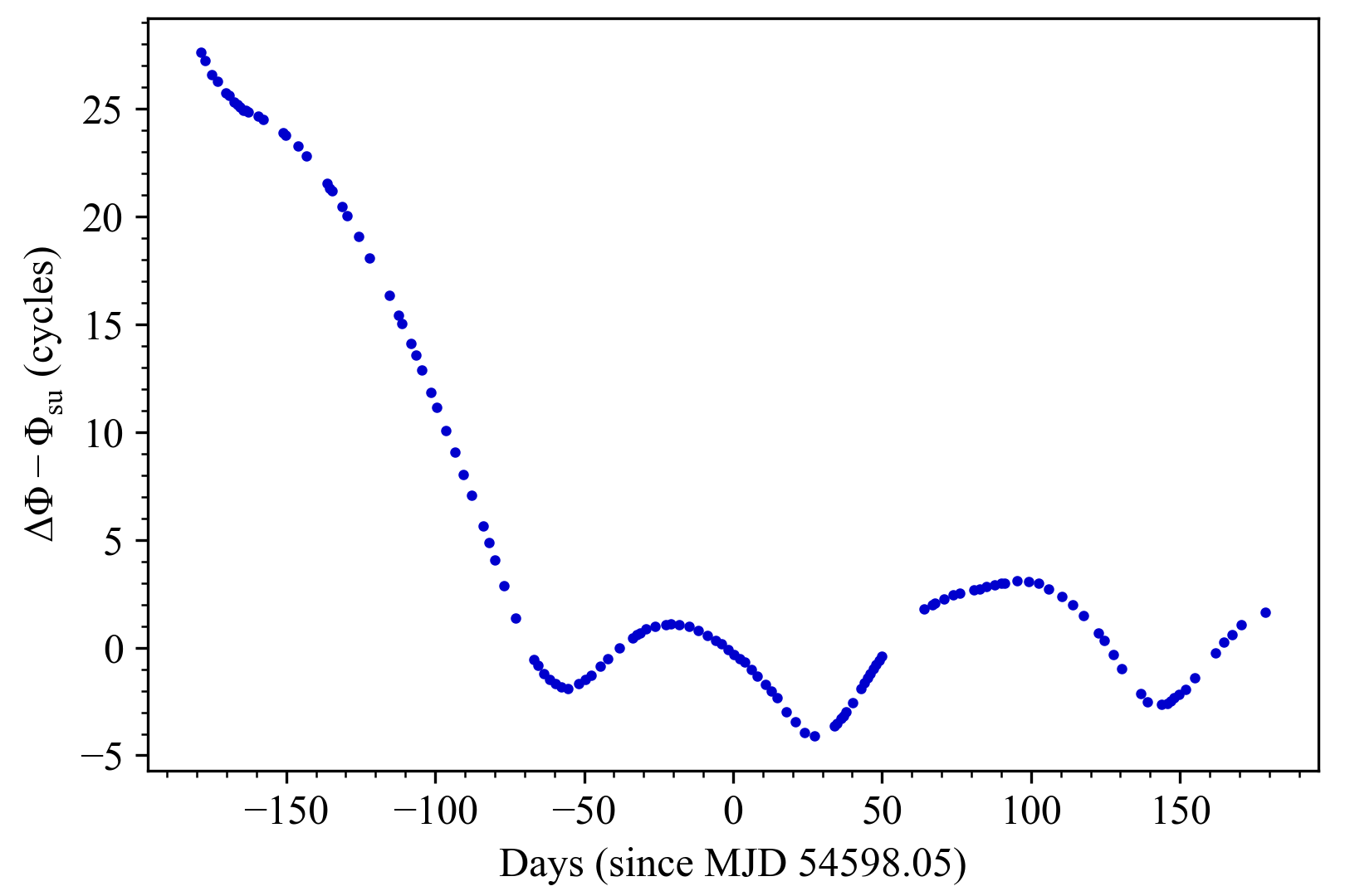
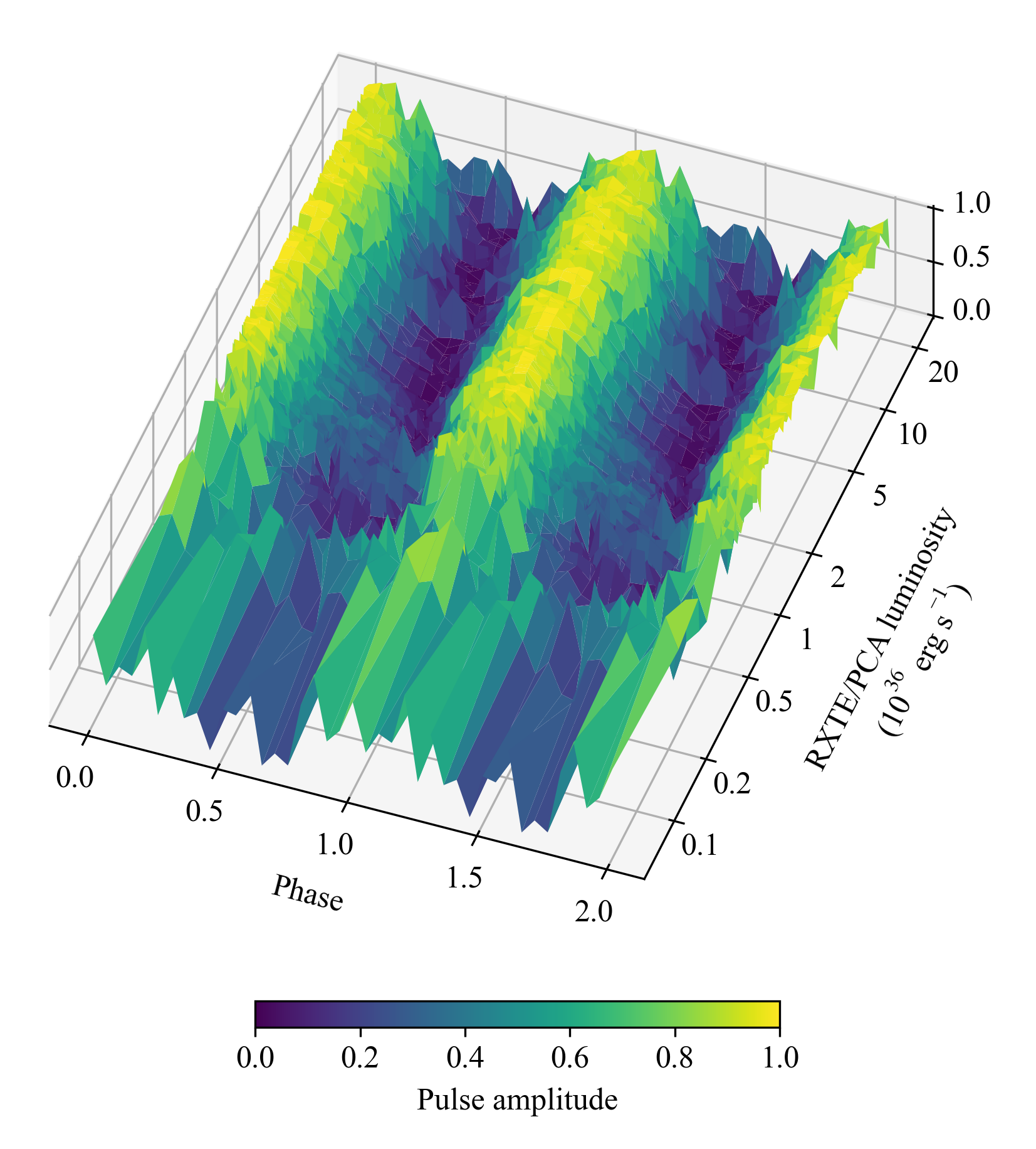
Figure 1: Left-hand panel: The pulse TOAs obtained from the RXTE/PCA observations after the removal of the overall spin-up trend (see text). Right-hand panel: Pulse profile evolution of MXB 0656–072, sorted by 3-20 keV RXTE/PCA luminosity. In order to improve legibility, the pulse profiles have been normalised to [0, 1] range and displayed for two complete cycles.

As the source continues to accrete, the pulse TOAs rapidly drift, especially due to enhanced accretion episodes at the type I outbursts within the analysis interval. Therefore, we represent the pulse TOAs after the removal of the overall spin-up trend, $\Phi_{\mathrm{su}}$, starting at Epoch = MJD 54598.05, with $\nu=6.27128(6)$ mHz and $\dot{\nu}=1.14(2)\times 10^{-12}$ Hz s^-1. Noting the complex time evolution of the pulse TOAs even after elimination of the spin-up trend (Figure 1), we do not characterise them with high-order polynomials to specify a phase-coherent timing solution. Instead, we directly convert them into spin frequency measurements by fitting linear functions to every sequential TOA triplet. The slope of these linear functions are utilised to calculate the frequency corrections at the middle times of TOA triplets by $\delta\nu=\delta\phi/\delta t$ over the spin-up trend mentioned above. The resulting spin frequency history generated from the RXTE/PCA observations is illustrated in Figure 3 together with the Fermi/GBM measurements. The uncertainties of the frequency measurements are evaluated from the $1\sigma$ error ranges of the slope obtained during the fitting; and the horizontal uncertainties reflect the time range of TOA triplets contained therein.

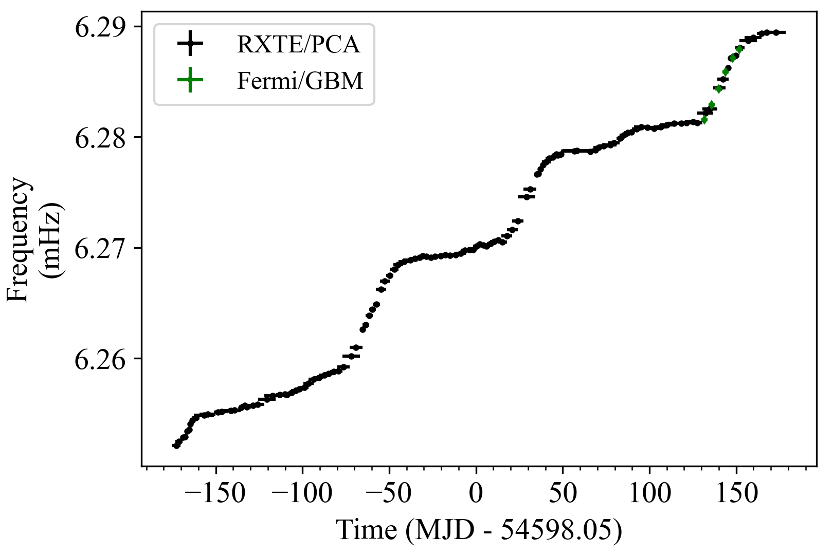
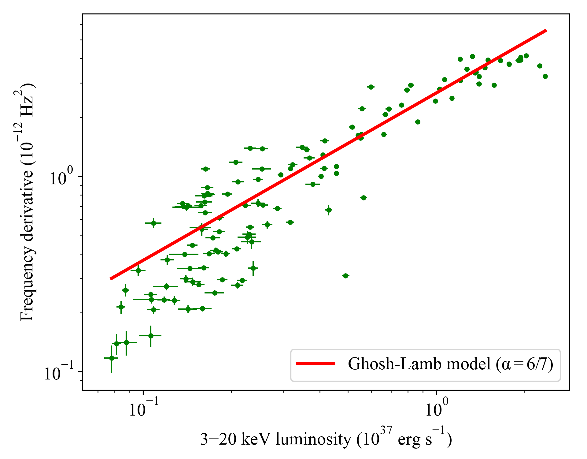
Figure 2: Left-hand panel: The spin frequency history of MXB 0656–072 obtained with RXTE/PCA (black points, this work) and Fermi/GBM (green diamonds). Right-hand panel: The distribution of spin-up rate measurements as a function of 3–20 keV RXTE/PCA luminosity of MXB 0656–072. The red line describes the best fit of the model.

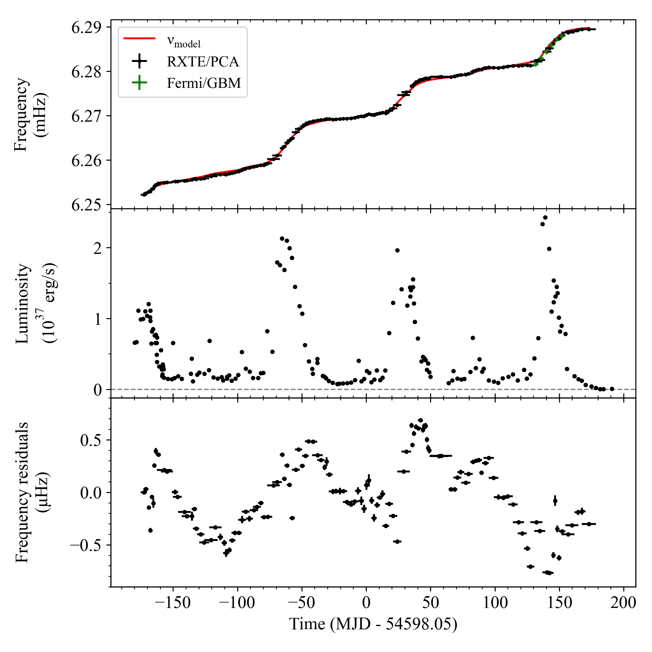
Figure 3: Upper panel: Frequency measurements of MXB 0656–072 with RXTE/PCA (black) and Fermi/GBM (green). The solid red line represents the intrinsic spin frequency model obtained through the $\dot{\nu}$–$L$ relation. Middle panel: 3–20 keV RXTE/PCA flux evolution. Lower panel: The spin frequency residuals after subtracting $\nu_{\textrm{model}}$ from the frequency measurements.

As it can be seen from Figure 1, MXB 0656–072 always spins up during the year, covered by the observations analysed in our study. Even though the spin frequencies seem to modulate at the suggested orbital period ($\sim$101.2 days; Yan et al., 2012) over a general spin-up trend, they should be examined with caution. The spin-up rate enhancements correspond to the bursting episodes, yet the spin-up trend still persists at rather quiescent episodes between the type I outbursts. Thus, we examine the intrinsic spin frequency evolution due to the torque exerted on the pulsar via accretion. The spin frequency derivatives are calculated first, using sequential linear fits to $\sim$20-day-long segments in the frequency history in a similar procedure as described above. Next, a linear spline interpolation of the RXTE/PCA flux evolution is used in order to estimate the flux range corresponding to the intervals where the spin frequency derivatives are measured. The distribution of measured spin-up rates with respect to the flux exhibits a clear correlation (see Figure 2), as expected from torque models (e.g., Ghosh & Lamb (1979); Lovelace et al. (1995); Kluźniak & Rappaport (2007)). Considering the Ghosh–Lamb model, the correlation is modelled with a power law relation (i.e., $\dot{\nu}_{12}=\beta\,L^{6/7}_{37}$). The best fit yields $\beta=2.42(6)$ (1$\sigma$ confidence level). Then, the intrinsic spin frequency evolution, which originates from the accretion, is constructed as (Serim et al., 2022):

$$\nu_{\mathrm{model}}(t)=\nu_{0}+\int_{t_{0}}^{t_{f}}\beta L(t^{\prime})^{6/7}dt^{\prime}$$ (1)

where $t_{0}$ and $t_{f}$ denote the start and end times of the data set, and $\nu_{0}$ is the spin frequency at $t_{0}$. Figure 3 displays the intrinsic spin frequency evolution in concert with the measured frequency set and its residuals. The residuals possess some structural variations; however, they do not seem to exhibit a clear sign for modulation due to orbital motion. Consequently, we are not able to constrain the orbital parameters of MXB 0656–072 with this data set.

4 Timing Noise Phenomenon

Timing noise is defined as the stochastic wandering in the residuals after fitting the data with an appropriate model. There are different metrics to interpolate the timing noise amplitudes of pulsars (e.g., see Deeter & Boynton, 1985; Arzoumanian et al., 1994; Shannon & Cordes, 2010; Lower et al., 2020; Jones et al., 2023), and although there are numerous studies focusing on theoretical framework of underlying physical processes (e.g., see Meyers et al., 2021a; Meyers et al., 2021b; Antonelli et al., 2023; Vargas & Melatos, 2023, and references therein), the timing noise phenomenon is still poorly understood. In recent years, studies on timing noise have become especially important in the detection of gravitational waves (e.g., see Riles, 2023, and references therein). Time-dependent noise characteristics of a pulsar provide hints for ongoing physical processes specific to that pulsar. For example, in a binary system, timing noise at viscous time-scales are dominated by the torque fluctuations associated with accretion flow (Serim et al., 2023a). On the other hand, isolated pulsars are found to exhibit higher timing noise levels at lower characteristic ages and their timing noise behaviours are mostly associated with rotational instabilities and magnetospheric fluctuations (Hobbs et al., 2010; Çerri-Serim et al., 2019).

The spin frequency history of MXB 0656–072 obtained in this work has a data sampling rate of 1 measurement per $\sim$3 days. This is achieved through the comprehensive monitoring campaign conducted with RXTE/PCA, which provides an ideal input for timing noise analysis at moderate time-scales. In order to understand the timing noise behaviour of the source at different time-scales, three different techniques are employed. The first technique utilises the root mean square (rms) values of the residuals after eliminating a polynomial of order $m$ from the input data spanning a time coverage of $T_{max}$ (Boynton et al., 1972; Deeter, 1984; Cordes & Downs, 1985). In this case, the rms $\langle\sigma_{r}(m,T)\rangle$ values can be linked with a noise strength $S_{r}$ for an input data of duration $T$ using the expression:

$$S_{r}=\frac{\langle\sigma_{r}(m,T)\rangle}{\langle\sigma_{r}(m,1)\rangle_{u}}\frac{1}{T^{2r-1}}$$ (2)

where the subscript $r$ reflects the order of the red noise. The coefficient $\langle\sigma_{r}(m,1)\rangle_{u}$ contains appropriate normalisation factors for the unit timing noise strength $S_{r}$ on a unit time-scale $T=1$, which can be obtained via direct evaluations (Deeter, 1984, Table 1). Then, noise strength calculations are repeated for different time-scales (i.e., $T_{max}/2^{n}$ for $n=1,2,3...$); and they are logarithmically combined across each time-scale to acquire the corresponding power density estimate. This technique enables the construction of a computationally less expensive low-resolution power density spectra (PDS) for torque fluctuations. Afterwards, we further employ two new PDS generation techniques based on the temporal changes of the long-term noise strength estimators in the literature with an aim of improving the PDS resolution.

In the second technique, we employ the noise strength estimation method introduced by Arzoumanian et al. (1994), which utilises the timing parameters obtained by fitting the input TOA or frequency set for a certain time-scale. In this case, the noise strength amplitudes are approximated using the spin frequency and its second order derivative as:

$$\Delta(T)=\textrm{log}\bigg{(}\frac{|\ddot{\nu}|T^{3}}{6\nu}\bigg{)}$$ (3)

where $\ddot{\nu}$ represents the second derivative of the pulse frequency $\nu$. In the literature, this method is used to calculate the noise strengths of many pulsars at the same time-scale for comparison (e.g., Arzoumanian et al., 1994; Hobbs et al., 2010; Andersen et al., 2023; Zhou et al., 2023). The reference time-scale for such comparisons is usually set to 10⁸ s to examine long-term noise correlations (Arzoumanian et al., 1994), and hence the parameter is generally referred to as $\Delta_{8}$. In order to trace the temporal noise behaviour of the source with this method, we use 10^Δ as the noise amplitude metric on the time-scale T. The results are rescaled with a factor of $1.1\times 10^{-19}$ s^-4 by crossfitting the noise amplitudes obtained from the Deeter method, with the sole aim of comparing the PDS profiles.

The third technique we used for noise strength estimation is the $\sigma_{z}$ method developed by Matsakis et al. (1997). In this method, Allan variance of the residuals after the removal of the regular frequency evolution trend up to the $\ddot{\nu}$ term (with the polynomial description) is assumed to govern the timing noise. $\sigma_{z}$ can be calculated as below:

$$\sigma_{z}=\frac{2}{\sqrt{5}}\frac{\langle\sigma_{\ddot{\nu}}\rangle}{\nu}$$ (4)

In this notation, $\langle\sigma_{\ddot{\nu}}\rangle$ has correspondence to $\langle\sigma_{1}(2,T)\rangle$ in the above description for the Deeter method, with a time-scale-dependent renormalisation ratio of $2T\langle\sigma_{r}(m,1)\rangle_{u}/\sqrt{5}\nu$ for $\sigma_{z}$. Similar to $\Delta(T)$, $\sigma_{z}$ is also often used for investigating long-term correlations among large pulsar populations.

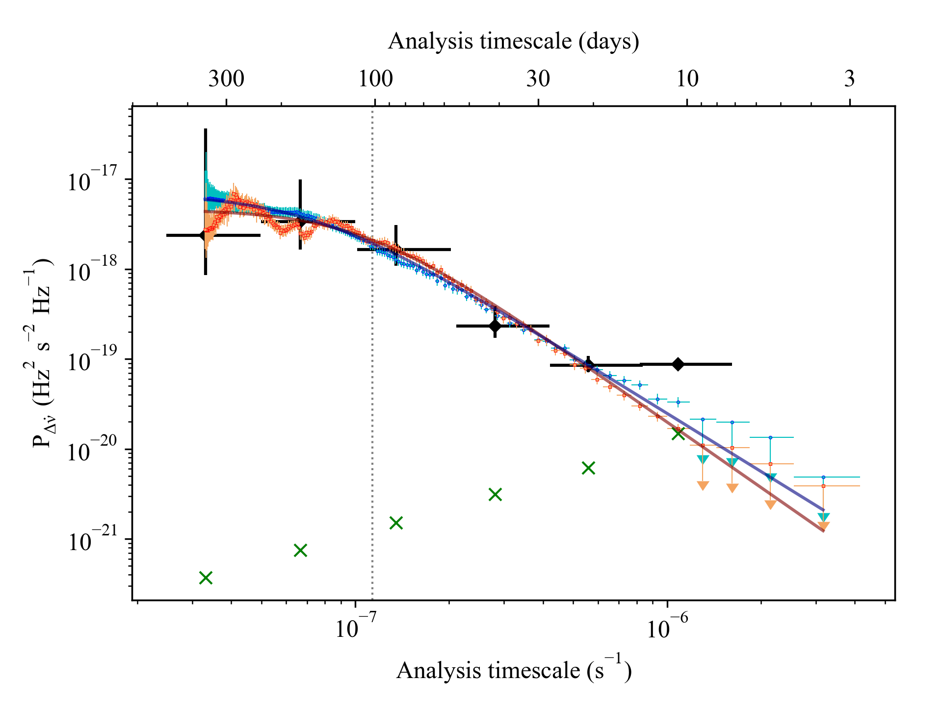
Figure 4: The PDS of the torque fluctuations of MXB 0656–072 obtained via Deeter method (black dots), Delta-parameter variation (orange dots) and $\sigma_{z}$-variation (blue dots). Dark red and dark blue lines represent the best fit model for Delta-parameter and $\sigma_{z}$ variations using the model described through Equation 6. The vertical dotted line indicates the orbital time-scale suggested by Yan et al. (2012).

To generate high-resolution PDSs for the latter two techniques, we calculate the noise strength amplitudes for temporal combinations in all of the possible time-scales allowed by the input frequency data set. In order to eliminate the possible outliers in the noise strength estimators, the estimators are filtered for valid fitting parameters. The estimators undergo additional screening for measuremental noise strength levels that are associated with the uncertainities $\sigma_{i}$ of the input data set. The measuremental noise strength level (MNS) in this case is calculated by:

$$\textrm{MNS}(T)=\frac{\sum_{i}^{N}\sigma_{i}^{2}}{NT\langle\sigma_{r}(m,1)\rangle_{u}}$$ (5)

where $N$ is the total number of measurements, and $\langle\sigma_{r}(m,1)\rangle_{u}$ is the normalisation factor described above. Then, the noise strength estimators are rebinned into power density estimators to construct the PDSs. As suggested by Matsakis et al. (1997), the uncertainty ranges ($\delta_{\pm}$) of the power density estimators can be obtained from $\chi^{2}$ distributions for $n$ degrees of freedom, which are specified by the number of noise estimations therein. However, this error estimate is only applicable for independent non-overlapping segments at low $n$ (Matsakis et al., 1997, see their Appendix A for details). The uncertainty ranges of the overlapping segments with a large number of measurements are dominated by the standard error ($SE$) of the noise estimations. Therefore, we used the combined error $\sqrt{\delta_{\pm}^{2}+SE^{2}}$ to approximate the propagating uncertainties of the power density estimators. Figure 4 illustrates the PDSs resulting from the aforementioned three distinct techniques.

All the generated PDSs exhibit consistency across various time-scales, with the exception of a slight difference at shorter time-scales ($\lesssim$20 days). In all cases, the presence of a red noise structure is clearly discernible, with a tendency to saturate at longer time-scales ($\gtrsim$150 days). This behavior is reminiscent of observations in 2S 1417–624 (Serim et al., 2022), Her X-1, and Cen X-3 (Bildsten et al., 1997; Serim et al., 2023a). The PDS continuum of MXB 0656–072 aligns with the generalized colored exponential shot noise model proposed by Burderi et al. (1997). As such, we model the PDSs of torque fluctuations ($P_{\Delta\dot{\nu}}$) following the equation presented by (Burderi et al., 1997; Serim et al., 2023a):

$$P_{\Delta\dot{\nu}}=\frac{S_{r}}{1+(\omega/\omega_{b})^{\Gamma}}.$$ (6)

In this equation, $\omega$ represents the analysis frequency, $\omega_{b}$ stands for the break frequency that is induced by the decay time-scale of exponential torque shots, and $\Gamma$ reflects the power law index that mediates the arbitrary slope triggered by the red noise process. The results of the model fitting for all the PDSs are depicted in Figure 4 and the corresponding parameters are provided in Table 1. Upon comparison, the latter two methods seem to provide an edge over the Deeter method: These methods yield PDSs with better resolution, particularly at higher frequencies. The PDS modeling reveals a power law index of $\sim$-2, implying that the red noise continuum possibly originates from a monochromatic shot noise sequence rather than a colored event sequence (i.e., torque events with varying time-scales).

Table 1: The parameters obtained from PDS modeling through Equation 6.

	$\Delta$-method	$\sigma_{z}$-method	Unit
$S_{r}$	$4.62(25)\times 10^{-18}$	$7.02(13)\times 10^{-18}$	Hz2 s-2 Hz-1
$\omega_{b}$	$1.05(7)\times 10^{-7}$	$7.21(15)\times 10^{-8}$	$s^{-1}$
$\Gamma$	-2.42(35)	-2.15(6)	-

5 Discussion and Conclusion

MXB 0656–072 is a relatively understudied member of the Be/X-ray binary class. We have revisited the type I outburst sequence that transpired during the period of 2007–2008, utilising observations from the RXTE/PCA instrument. The methodology employed in our analysis involves pulse timing, which enables us to determine the temporal evolution of the pulse frequency for the specified time interval. We discover a strong correlation between the spin frequency derivatives and source luminosity in the 3–20 keV band. Given the assumption that this luminosity in 3–20 keV band covers most of the bolometric luminosity in X-rays, the magnetic field strength can be estimated via torque models. For example, this estimation can be done through the use of the torque model introduced by Ghosh & Lamb (1979) via:

$$\dot{\nu}_{12}=1.4\mu_{30}^{2/7}n(\omega_{s})R_{6}^{6/7}M_{1.4}^{-3/7}I_{45}^{-1}L_{37}^{6/7}$$ (7)

where $\dot{\nu}$ is the spin-up rate, $\mu$ is the dipole moment, $n(\omega_{s})$ is the fastness parameter, $L$ is the bolometric X-ray luminosity, and $R$, $M$ and $I$ respectively denote the radius, mass and moment of inertia of the pulsar. Our best-fit torque-luminosity relation is represented by the equation $\dot{\nu}_{12}=2.42(6)\times L_{37}^{6/7}$ (assuming a distance of 5.7 kpc, as specified in Section 3). By employing typical neutron star parameters and the slow rotator approximation ($n(\omega_{s})\approx 1.4$), an estimation of the magnetic field strength of the source yields an approximate value of $4.2\times 10^{12}$ G. The calculated magnetic field strength is very close to, albeit slightly higher than, the values inferred from CRSF (Heindl et al., 2003). Nevertheless, it is crucial to note that the magnetic field strength calculations based on torque models are considerably affected by the luminosity of the source and, consequently, the estimated distance. Therefore, we also explore its coherence with alternative methodologies employed in the interpretation of magnetic field strength.

The first alternative estimation of the magnetic field strength relies on the CRSFs that MXB 0656–072 is known to exhibit within the energy interval of 30–36 keV, suggesting the presence of a dipolar magnetic field with an estimated strength of approximately $3.4-3.7\times 10^{12}$ G (Heindl et al., 2003; McBride et al., 2006a, b; Yan et al., 2012).

Considering another estimation, Nespoli et al. (2012) reported a potential flattening of the photon index above a luminosity threshold of $2.3\times 10^{37}$ erg s^-1, based on an assumed distance of 3.9 kpc. When adjusted for the Gaia EDR3 distance of 5.7 kpc, this luminosity corresponds to approximately $4.9\times 10^{37}$ erg s^-1. In other words, MXB 0656–072 exhibits an anti-correlative behaviour between photon index and luminosity when the latter is below $\sim$$4.9\times 10^{37}$ erg s^-1. The anti-correlation ceases beyond this luminosity threshold, resulting in photon indices becoming flattened (Nespoli et al., 2012). The critical luminosity at which spectral correlation turnover occurs can be considered as an onset for the transition from a pencil to a fan beam (e.g., Doroshenko et al., 2020; Serim et al., 2022; Rai et al., 2023; Mandal & Pal, 2023). Hence, the relationship between the critical luminosity and the magnetic field strength can be described as follows (Becker et al., 2012):

$$L_{\textrm{crit}}=1.5\times 10^{37}B_{12}^{16/15}\,\,\textrm{erg s}^{-1}.$$ (8)

Under the assumption that the aforementioned luminosity threshold corresponds to the critical luminosity for transition, the magnetic field strength can be obtained as $\sim$$3\times 10^{12}$ G.

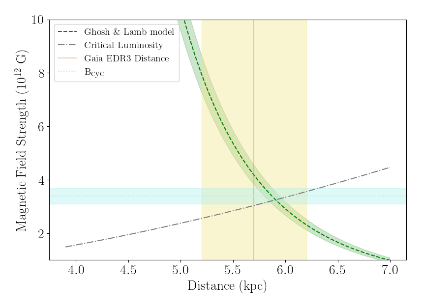
Figure 5: The magnetic field strength of MXB 0656–072 as a function of distance, deduced through various models. Shaded regions reflect the uncertainty range of measured/calculated parameters.

Even though there is a broad consensus in the magnetic field strength estimates, there is a slight discrepancy that might originate from the assumptions about distance (or bolometric luminosity). Therefore, we explore the dependency of magnetic field strengths on distance prescribed in Equation (7) and (8) in conjunction with the CSRF interpretation, presented in Figure 5. The figure illustrates that all models converge to the same region in the magnetic field strength vs. distance diagram. Hence, the distance of the system can be deduced to be $\sim$5.9 kpc, well within the uncertainty range of the Gaia distance estimate of $5.7\pm 0.5$ kpc. If that is the case, the magnetic field strength of MXB 0656–072 is expected to be approximately $3.3\times 10^{12}$ G, consistent with previous deductions based on CSRF (Yan et al., 2012).

It should be noted that the aforementioned interpretations are based on the assumption that the emission in the 3–20 keV range constitutes the majority of the bolometric luminosity. If this assumption leads to an underestimation of the source emission in higher energy bands, it is also viable to identify an alternative position on the magnetic field strength vs. distance diagram that coincides with the Gaia EDR3 distance and the B-field strength deduced from CSRF. Convergence at this specific position on the diagram requires that $\sim$92% of the bolometric luminosity is emitted in the 3–20 keV band.

Furthermore, we constructed and examined the long-term spin frequency evolution of the source over an almost one-year period. Overall, MXB 0656–072 undergoes spin-up during the type I outburst sequences that took place in 2007–2008. The trend in spin frequency can be accurately depicted by the intrinsic frequency evolution driven by accretion torques. Despite the structural variations in the residuals (see Figure 3, bottom panel), no distinct orbital modulation is evident. Hence, we are unable to uncover the orbital timing parameters from this data set. On the other hand, Yan et al. (2012) estimated the semimajor axis of the system as $253R_{\odot}$ by assuming an O9.7Ve companion of $20M_{\odot}$ and $15R_{\odot}$, considering its resemblance to A 0535+26. Given these assumptions, the semimajor axis of the system can be converted to 587 lt-s. Then, the maximum amplitude of frequency modulations $\delta\nu$ arising from orbital motion can be estimated as (Serim et al., 2017):

$$\delta\nu\sin i=\frac{2\pi}{P_{\textrm{orb}}}\frac{1}{P_{\textrm{spin}}}\frac{a}{c}\sin i$$ (9)

where $P_{\textrm{orb}}$ is the orbital period, $P_{\textrm{spin}}$ is the spin period, $a/c$ represents the semimajor axis, and $\sin i$ denotes inclination. By applying Equation (9), the maximum amplitude of frequency modulations can be derived as $\sim$2.6 $\mu$Hz. Nonetheless, the timing residuals in our analysis are constrained to an amplitude of $\sim$0.7 $\mu$Hz, suggesting that we are observing the system from a relatively "top view", with an inclination, $\sin i$, less than 0.27.

In addition, we performed an analysis of the PDS focusing on the variations in the spin frequency derivative of MXB 0656–072. Our investigation is centered on a robust spin frequency data set with measurements obtained every $\sim$3 days, gathered from new measurements acquired through our timing analysis of RXTE/PCA observations. Employing different methodologies, we generated three distinct PDS profiles to assess the temporal noise strength in the residuals. While the initial method involves the conventional Deeter method (Deeter, 1984); the other two methods ($\sigma_{z}$: Matsakis et al. 1997, $\Delta$-parameter: Arzoumanian et al. 1994), to the best of our knowledge, are first to be applied for detailed PDS extraction. The PDS profiles for MXB 0656–072 remain consistent across all these methods.

In a broader context, wind-fed sources exhibit a white noise pattern that is attributed to uncorrelated torque events produced by wind inhomogeneities. Typically, such wind-fed systems exhibit torque noise strengths within the range of $10^{-20}$–$10^{-18}$ Hz² s^-2 Hz^-1 (Bildsten et al., 1997). On the other hand, disc-fed sources rather exhibit a red noise pattern in their PDS in general, due to their torque evolution is being driven by a sequence of correlated events. Such red noise patterns generally evolve with $\omega^{-2}$ and reach saturation at long time-scales, potentially exceeding the viscous fluctuation time-scales in the disc (Içdem & Baykal, 2011). Analysis of PDS in such persistent systems with disc accretion indicates that their torque noise strengths typically reside between $10^{-21}$–$10^{-18}$ Hz² s^-2 Hz^-1 (Bildsten et al., 1997). The transient sources appear to share a similar nature in the PDS of torque fluctuations (Baykal et al., 2007; Serim et al., 2022), barring Swift J0243.6+6124, which stands out with a relatively steep PDS ($\sim$$\omega^{-3.36}$) and a presence of a white noise component at shorter time-scales (Serim et al., 2023b). Yet, the pronounced steepness in the PDS of Swift J0243.6+6124 is argued to stem from quadrupolar interactions occurring at elevated luminosities (Serim et al., 2023b). MXB 0656–072 exhibits a PDS profile akin to prior cases, such as Her X-1, Cen X-3 (Bildsten et al., 1997; Serim et al., 2023a), and 2S 1417–624 (Serim et al., 2022). It is characterised by a red noise component with a steepness of $\Gamma\sim-2$ reaching saturation over a time-scale of $\sim$150 days (see Table 1 for details). The measured torque noise strength values of MXB 0656–072 fall within the range of $1\times 10^{-20}$ to $7\times 10^{-18}$ Hz² s^-2 Hz^-1 across the analysis frequency span of $3.5\times 10^{-7}$ to $1\times 10^{-6}$ s^-1. This observed PDS profile is in line with the generalized colored exponential shot model (Burderi et al., 1997; Serim et al., 2023a), which characterizes an empirical model for the correlative sequence of events generated by accretion torques. Since the steepness of the PDS is roughly consistent with $\Gamma\sim-2$, the profile suggests a likelihood of a monochromatic sequence of torque events generated by stable disc accretion throughout the observed time frame.

The newly implemented methods also handle estimations of temporal noise strength across all possible combinations of time-scales within the input data, thereby providing improved PDS resolution, particularly at higher analysis frequencies. Despite our sampling rate remains restricted to 1 measurement per $\sim$3 days for MXB 0656–072, in principle, these methods have the potential to distinguish properties within PDS at higher analysis frequencies. Many studies in the literature focus on the theoretical aspects of the timing noise generation within a neutron star’s inner response under the influence of external torques (e.g., Alpar et al. (1986); Baykal et al. (1991); Baykal (1997); Gügercinoǧlu & Alpar (2017); Meyers et al. (2021a); Antonelli et al. (2023)). The expected timing noise contribution from the interior of a neutron star under such conditions is anticipated to be revealed at crust–core coupling time-scales, approximately spanning from 10 to 100 rotational periods (Sidery & Alpar, 2009). Therefore, the techniques introduced in this paper could potentially enable the investigation of the PDS structure at higher analysis frequencies, thus providing an avenue to study neutron star interior through timing noise, given that the data sampling rate is adequate.

Data Availability

The whole X-ray data used in this study is publicly available. NICER/XTI data can be obtained through the High Energy Astrophysics Science Archive Research Center website (https://heasarc.gsfc.nasa.gov). Fermi/GBM frequency measurements are available at GBM Accreting Pulsars Project website (https://gammaray.msfc.nasa.gov/gbm/science/pulsars.html).

References

- Alpar et al. (1986) Alpar M. A., Nandkumar R., Pines D., 1986, ApJ, 311, 197
- Andersen et al. (2023) Andersen B. C., et al., 2023, ApJ, 943, 57
- Antonelli et al. (2023) Antonelli M., Basu A., Haskell B., 2023, MNRAS, 520, 2813
- Arzoumanian et al. (1994) Arzoumanian Z., Nice D. J., Taylor J. H., Thorsett S. E., 1994, ApJ, 422, 671
- Baykal (1997) Baykal A., 1997, A&A, 319, 515
- Baykal et al. (1991) Baykal A., Alpar A., Kiziloglu U., 1991, A&A, 252, 664
- Baykal et al. (2007) Baykal A., Inam S. Ç., Stark M. J., Heffner C. M., Erkoca A. E., Swank J. H., 2007, MNRAS, 374, 1108
- Becker et al. (2012) Becker P. A., et al., 2012, A&A, 544, A123
- Bildsten et al. (1997) Bildsten L., et al., 1997, ApJS, 113, 367
- Boynton et al. (1972) Boynton P. E., Groth E. J., Hutchinson D. P., Nanos G. P. J., Partridge R. B., Wilkinson D. T., 1972, ApJ, 175, 217
- Burderi et al. (1997) Burderi L., Robba N. R., La Barbera N., Guainazzi M., 1997, ApJ, 481, 943
- Clark et al. (1975) Clark G. W., Schmidt G. D., Angel J. R. P., 1975, IAU Circ., 2843, 1
- Cordes & Downs (1985) Cordes J. M., Downs G. S., 1985, ApJS, 59, 343
- Deeter (1984) Deeter J. E., 1984, ApJ, 281, 482
- Deeter & Boynton (1985) Deeter J. E., Boynton P. E., 1985, in Hayakawa S. and Nagase F. Proc. Inuyama Workshop: Timing Studies of X-Ray Sources p.29, Nagoya Univ., Nagoya
- Doroshenko et al. (2020) Doroshenko V., et al., 2020, MNRAS, 491, 1857
- Gaia Collaboration et al. (2016) Gaia Collaboration et al., 2016, A&A, 595, A1
- Gaia Collaboration et al. (2021) Gaia Collaboration et al., 2021, A&A, 649, A1
- Ghosh & Lamb (1979) Ghosh P., Lamb F. K., 1979, ApJ, 234, 296
- Gügercinoǧlu & Alpar (2017) Gügercinoǧlu E., Alpar M. A., 2017, MNRAS, 471, 4827
- Heindl et al. (2003) Heindl W., Coburn W., Kreykenbohm I., Wilms J., 2003, The Astronomer’s Telegram, 200, 1
- Hobbs et al. (2010) Hobbs G., Lyne A. G., Kramer M., 2010, MNRAS, 402, 1027
- Içdem & Baykal (2011) Içdem B., Baykal A., 2011, A&A, 529, A7
- Jahoda et al. (1996) Jahoda K., Swank J. H., Giles A. B., Stark M. J., Strohmayer T., Zhang W., Morgan E. H., 1996, in Siegmund O. H., Gummin M. A., eds, Society of Photo-Optical Instrumentation Engineers (SPIE) Conference Series Vol. 2808, EUV, X-Ray, and Gamma-Ray Instrumentation for Astronomy VII. pp 59–70, doi:10.1117/12.256034
- Jones et al. (2023) Jones M. L., Kaplan D. L., McLaughlin M. A., Lorimer D. R., 2023, ApJ, 951, 20
- Kennea et al. (2007) Kennea J. A., Romano P., Pottschmidt K., Wilms J., Cummings J., Evans P., Burrows D. N., 2007, The Astronomer’s Telegram, 1293, 1
- Kluźniak & Rappaport (2007) Kluźniak W., Rappaport S., 2007, ApJ, 671, 1990
- Kreykenbohm et al. (2007) Kreykenbohm I., et al., 2007, The Astronomer’s Telegram, 1281, 1
- Leahy et al. (1983) Leahy D. A., Darbro W., Elsner R. F., Weisskopf M. C., Sutherland P. G., Kahn S., Grindlay J. E., 1983, ApJ, 266, 160
- Lovelace et al. (1995) Lovelace R. V. E., Romanova M. M., Bisnovatyi-Kogan G. S., 1995, MNRAS, 275, 244
- Lower et al. (2020) Lower M. E., et al., 2020, MNRAS, 494, 228
- Mandal & Pal (2023) Mandal M., Pal S., 2023, Journal of Astrophysics and Astronomy, 44, 60
- Matsakis et al. (1997) Matsakis D. N., Taylor J. H., Eubanks T. M., 1997, A&A, 326, 924
- McBride et al. (2006a) McBride V. A., Coburn W., Coe M. J., Kretschmar P., Kreykenbohm I., Rothschild R. E., Staubert R., Wilms J., 2006a, Advances in Space Research, 38, 2768
- McBride et al. (2006b) McBride V. A., et al., 2006b, A&A, 451, 267
- Meyers et al. (2021a) Meyers P. M., Melatos A., O’Neill N. J., 2021a, MNRAS, 502, 3113
- Meyers et al. (2021b) Meyers P. M., O’Neill N. J., Melatos A., Evans R. J., 2021b, MNRAS, 506, 3349
- Morgan et al. (2003) Morgan E., Remillard R., Swank J., 2003, The Astronomer’s Telegram, 199, 1
- Nespoli et al. (2012) Nespoli E., Reig P., Zezas A., 2012, A&A, 547, A103
- Pakull et al. (2003) Pakull M. W., Motch C., Negueruela I., 2003, The Astronomer’s Telegram, 202, 1
- Pottschmidt et al. (2007) Pottschmidt K., et al., 2007, The Astronomer’s Telegram, 1283, 1
- Rai et al. (2023) Rai B., Paul B., Tobrej M., Ghising M., Tamang R., Paul B. C., 2023, Journal of Astrophysics and Astronomy, 44, 39
- Raman et al. (2023) Raman G., Varun Pradhan P., Kennea J., 2023, arXiv e-prints, p. arXiv:2308.12498
- Reig (2011) Reig P., 2011, Ap&SS, 332, 1
- Riles (2023) Riles K., 2023, Living Reviews in Relativity, 26, 3
- Serim et al. (2017) Serim M. M., Şahiner Ş., Çerri-Serim D., İnam S. Ç., Baykal A., 2017, MNRAS, 469, 2509
- Serim et al. (2022) Serim M. M., Özüdoğru Ö. C., Dönmez Ç. K., Şahiner Ş., Serim D., Baykal A., İnam S. Ç., 2022, MNRAS, 510, 1438
- Serim et al. (2023a) Serim D., Serim M. M., Baykal A., 2023a, MNRAS, 518, 1
- Serim et al. (2023b) Serim M. M., Dönmez Ç. K., Serim D., Ducci L., Baykal A., Santangelo A., 2023b, MNRAS, 522, 6115
- Shannon & Cordes (2010) Shannon R. M., Cordes J. M., 2010, ApJ, 725, 1607
- Sidery & Alpar (2009) Sidery T., Alpar M. A., 2009, MNRAS, 400, 1859
- Tsygankov et al. (2017) Tsygankov S. S., Wijnands R., Lutovinov A. A., Degenaar N., Poutanen J., 2017, MNRAS, 470, 126
- Vargas & Melatos (2023) Vargas A. F., Melatos A., 2023, MNRAS, 522, 4880
- Yan et al. (2012) Yan J., Zurita Heras J. A., Chaty S., Li H., Liu Q., 2012, ApJ, 753, 73
- Zhou et al. (2023) Zhou S. Q., et al., 2023, MNRAS, 519, 74
- Çerri-Serim et al. (2019) Çerri-Serim D., Serim M. M., Şahiner Ş., Inam S. Ç., Baykal A., 2019, MNRAS, 485, 2