MLMC: Machine Learning Monte Carlo for Lattice Gauge Theory

Abstract

We present a trainable framework for efficiently generating gauge configurations, and discuss ongoing work in this direction. In particular, we consider the problem of sampling configurations from a 4D $SU(3)$ lattice gauge theory, and consider a generalized leapfrog integrator in the molecular dynamics update that can be trained to improve sampling efficiency. Code is available online at l2hmc-qcd.

1 Introduction

We would like to calculate observables $\mathcal{O}$:

$$\left\langle\mathcal{O}\right\rangle\propto\int\left[\mathcal{D}x\right]\,\mathcal{O}(x)\,\pi(x)$$ (1)

where $\pi(x)\propto e^{-\beta S(x)}$ is our target distribution. If these were independent, we could approximate the integral as $\left\langle\mathcal{O}\right\rangle\simeq\frac{1}{N}\sum_{n=1}^{N}\mathcal{O}(x_{n})$ with variance

$$\sigma_{\mathcal{O}}^{2}=\frac{1}{N}\,\mathrm{Var}\left[\mathcal{O}(x)\right]\Longrightarrow\sigma_{\mathcal{O}}\propto\frac{1}{\sqrt{N}}.$$ (2)

Instead, nearby configurations are correlated, causing us to incur a factor of $\tau_{\mathrm{int}}^{\mathcal{O}}$ in the variance expression

$$\sigma_{\mathcal{O}}^{2}=\frac{\tau_{\mathrm{int}}^{\mathcal{O}}}{N}\mathrm{Var}\left[\mathcal{O}(x)\right].$$ (3)

1.1 Hamiltonian Monte Carlo (HMC)

The typical approach [8, 9] is to use Hamiltonian Monte Carlo (HMC) algorithm for generating configurations distributed according to our target distribution $\pi(x)$. This can be done by sequentially constructing a chain of states $\{x_{0},\,x_{1},\,x_{2},\,\ldots,\,x_{i},\,\ldots,\,x_{n}\}$, such that, as $n\rightarrow\infty$:

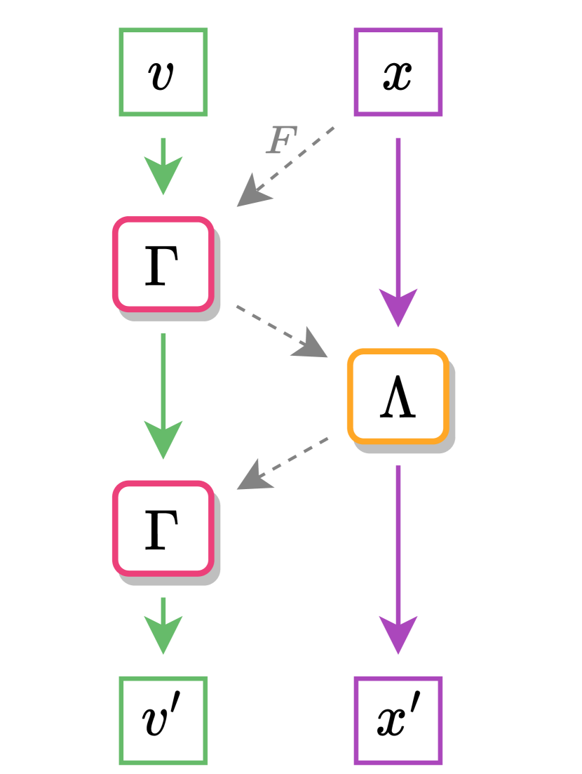
Figure 1: Leapfrog update.

$$\left\{x_{i},x_{i+1},x_{i+2},\ldots,x_{n}\right\}\sim\pi(x).$$ (4)

To do this, we begin by introducing a fictitious momentum $v\sim\mathcal{N}(0,1)$ normally distributed, independent of $x$. We can write the joint distribution $\pi(x,v)$ as

$$\pi(x,v) =\pi(x)\pi(v)\propto e^{-S(x)}e^{-\frac{1}{2}v^{T}v}$$ (5)

$$=e^{-\left[S(x)+\frac{1}{2}v^{T}v\right]}$$ (6)

We can evolve the Hamiltonian dynamics of the $(\dot{x},\dot{v})=(\partial_{v}H,-\partial_{x}H)$ system using operators $\Gamma:v\rightarrow v^{\prime}$ and $\Lambda:x\rightarrow x^{\prime}$. Explicitly, for a single update step of the leapfrog integrator:

$$\tilde{v} \coloneqq\Gamma(x,v)=v-\frac{\varepsilon}{2}F(x)$$ (7)

$$x^{\prime} \coloneqq\Lambda(x,\tilde{v})=x+\varepsilon\tilde{v}$$ (8)

$$v^{\prime} \coloneqq\Lambda(x^{\prime},\tilde{v})=\tilde{v}-\frac{\varepsilon}{2}F(x^{\prime}),$$ (9)

where we’ve written the force term as $F(x)=\partial_{x}S(x)$. Typically, we build a trajectory of $N_{\mathrm{LF}}$ leapfrog steps $(x_{0},v_{0})\rightarrow(x_{1},v_{1})\rightarrow\cdots\rightarrow(x^{\prime},v^{\prime}),$ and propose $x^{\prime}$ as the next state in our chain. This proposal state is then accepted according to the Metropolis-Hastings criteria [25]

$$A(x^{\prime}|x)=\mathrm{min}\left\{{1,\frac{\pi(x^{\prime})}{\pi(x)}\left|\frac{\partial x^{\prime}}{\partial x}\right|}\right\}.$$ (10)

2 Method

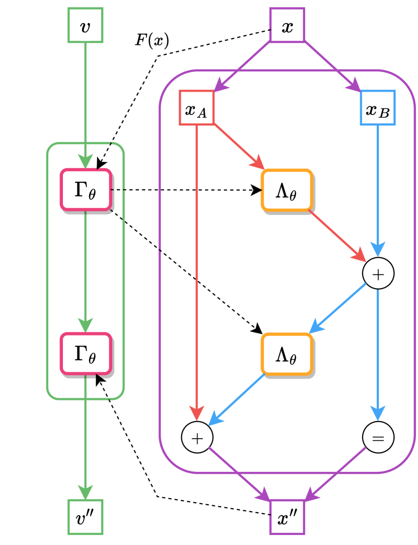
Figure 2: Generalized MD update.

Unfortunately, HMC is known to suffer from long auto-correlations and often struggles with multi-modal target densities. To combat this, we propose building on the approach from [10, 8, 9]. We introduce two (invertible) neural networks $\texttt{xNet}:(x,v)\rightarrow(\alpha_{x},\beta_{x},\gamma_{x})$, $\texttt{vNet}:(x,F)\rightarrow(\alpha_{v},\beta_{v},\gamma_{v})$.

Here, $\left(\alpha,\beta,\gamma\right)$ are all of the same dimensionality as $x$ and $v$, and are parameterized by a set of weights $\theta$. These network outputs $(\alpha,\beta,\gamma)$ are then used in a generalized MD update (as shown in Fig 2) via: where the superscript $\pm$ on $\Gamma^{\pm}_{\theta}$, $\Lambda^{\pm}_{\theta}$ correspond to the direction $d\sim\mathcal{U}(-1,+1)$ of the update.

To ensure that our proposed update remains reversible, we split the $x$ update into two sub-updates on complementary subsets ($x=x_{A}\cup x_{B}$):

$${v^{\prime}} ={\Gamma^{\pm}_{\theta}(x,v)}$$ (11)

$${x^{\prime}} =x_{B}+{\Lambda^{\pm}_{\theta}(x_{A},v^{\prime})}$$ (12)

$${x^{\prime\prime}} =x^{\prime}_{A}+{\Lambda^{\pm}_{\theta}(x^{\prime}_{B},v^{\prime})}$$ (13)

$${v^{\prime\prime}} ={\Gamma^{\pm}_{\theta}(x^{\prime\prime},v^{\prime})}$$ (14)

2.1 Algorithm

1. input: $x$

   • Re-sample $v\sim\mathcal{N}(0,1)$

   • Construct initial state $\xi\coloneqq(x,v)$

2. forward: Generate proposal $\xi^{\prime}$ by passing initial $\xi$ through $N_{\mathrm{LF}}$ leapfrog layers:

   $$\xi\xrightarrow[]{\mathrm{LF\,\,\,Layer}}\xi_{1}\rightarrow\cdots\rightarrow\xi_{N_{\mathrm{LF}}}=\xi^{\prime}\coloneqq(x^{\prime\prime},v^{\prime\prime})$$ (15)

   • Metropolis-Hastings accept / reject:

     $$A(\xi^{\prime}|\xi)=\mathrm{min}\left\{1,\frac{\pi(\xi^{\prime})}{\pi(\xi)}\left|\mathcal{J}\left(\xi^{\prime},\xi\right)\right|\right\},$$ (16)

     where $\left|\mathcal{J}(\xi^{\prime},\xi)\right|$ is the determinant of the Jacobian.

3. backward: (if training)

   • Evaluate the loss function $\mathcal{L}(\xi^{\prime},\xi)$ and back propagate

4. return: $x_{i+1}$

   • Evaluate MH criteria (Eq. 16) and return accepted config:

     $$x_{i+1}\leftarrow\begin{cases}x^{\prime\prime}\quad\text{w/ prob.}\quad A(\xi^{\prime}|\xi)\\ x\,\,\,\quad\text{w/ prob.}\quad 1-A(\xi^{\prime}|\xi)\end{cases}$$ (17)

3 Lattice Gauge Theories

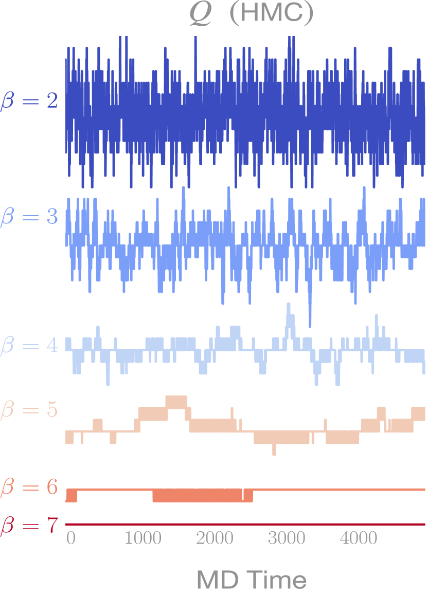
Figure 3: $\delta Q\rightarrow 0$ with increasing $\beta$ for the 2D $U(1)$ model. Image from [9].

3.1 2D $U(1)$ Model

We build upon the approach originally introduced in [17], which was successfully applied to the 2D $U(1)$ lattice gauge model in [10, 8, 9]. In particular, we are interested in measuring the (scalar) topological charge $Q\in\mathbb{Z}$ on the lattice. Since different lattice configurations with the same value of $Q$ are related by a gauge transformation, they do not meaningfully contribute to our statistics.

Because of this, we would like to generate configurations from different topological sectors (characterized by different values of $Q$) to reduce uncertainty in our statistical estimates. By repeating this procedure at increasing spatial resolution ($\beta\propto 1/a$), we are able to extrapolate our estimates to the continuum limit where they can be compared with experimental measurements. Current approaches such as HMC are known to suffer from auto-correlation times which scale exponentially in this limit, significantly limiting their effectiveness. This phenomenon can be seen in Fig 3, where fluctuations in the topological charge between sequential configurations (the tunneling rate) $\delta Q=|Q^{i+1}-Q^{i}|$ decreases as $\beta=2\rightarrow 3\rightarrow\cdots$, and disappear completely ($Q=\mathrm{const.}$) by $\beta=7$.

3.1.1 Results

Results for the 2D $U(1)$ model trained at $\beta=4$ in $\simeq 25$ minutes on a single NVIDIA A100 GPU, using l2hmc-qcd. We provide the full blue book Jupyter notebook containing the results in Fig 4.

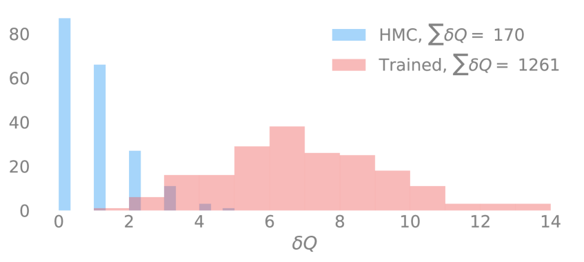
((a)) $\delta Q$ for trained model (red) vs HMC (blue).

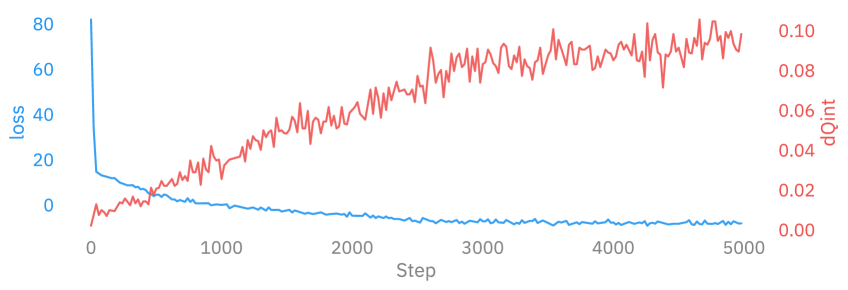
((b)) Loss (blue) and $\delta Q$ (red) during training

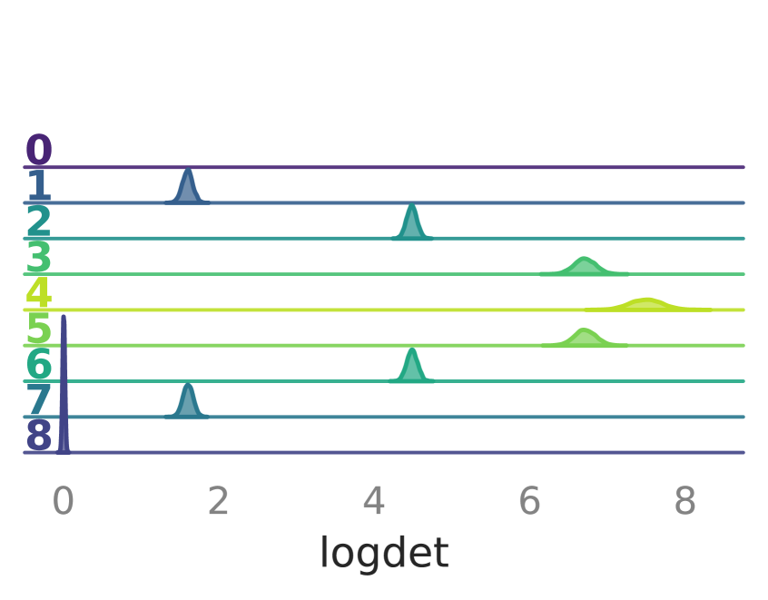
((c)) $|\mathcal{J}|$ vs LF step (trained)

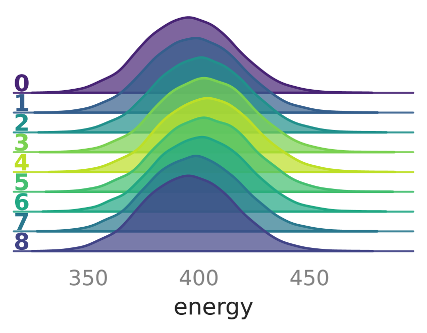
((d)) $H$ vs LF step (trained)

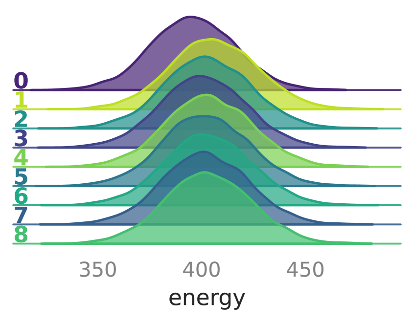
((e)) $H$ vs LF step (HMC)

Figure 4: Results from trained 2D $U(1)$ model at $\beta=4$. In 4(d) we see the energy $H$ increasing towards the middle of the trajectory, resulting in improved tunneling rate (larger $\delta Q$) in  4(a). blue book Jupyter notebook.

3.2 4D $SU(3)$ Model

We would like to generalize this approach to handle 4D $SU(3)$ link variables $U_{\mu}(n)\in SU(3)$:

$$U_{\mu}(n)=\exp\left[i\omega_{\mu}^{k}(n)\lambda^{k}\right]$$ (18)

where $\omega_{\mu}^{k}(n)\in\mathbb{R}$ and $\lambda^{k}$ are the generators of $SU(3)$. We consider the standard Wilson gauge action

$$S_{G} =-\frac{\beta}{6}\sum\mathrm{Tr}\left[U_{\mu\nu}(n)+U^{\dagger}_{\mu\nu}(n)\right],\quad\text{where}$$ (19)

$$U_{\mu\nu}(n) =U_{\mu}(n)U_{\nu}(n+\hat{\mu})U_{\mu}^{\dagger}(n+\hat{\nu})U^{\dagger}_{\nu}(n).$$ (20)

3.2.1 Generic MD Updates

As before, we introduce momenta $P_{\mu}(n)=P^{k}_{\mu}(n)\lambda^{k}$ conjugate to the real fields $\omega_{\mu}^{k}(n)$. We can write the Hamiltonian as

$$H[P,U]=\frac{1}{2}P^{2}+S_{G}[U]\Longrightarrow\kern 40.17522pt\kern-40.17522pt\fcolorbox{myGreen}{white}{\m@th$\displaystyle\frac{d\omega^{k}}{dt} = \frac{\partial H}{\partial P^{k}}$},\quad\kern 43.50854pt\kern-43.50854pt\fcolorbox{lfPurple}{white}{\m@th$\displaystyle\frac{dP^{k}}{dt} = - \frac{\partial H}{\partial\omega^{k}}$}.$$ (21)

To update the gauge field $U_{\mu}=e^{i\omega_{\mu}^{k}\lambda^{k}}$, write $\displaystyle\frac{d\omega^{k}}{dt}\lambda^{k}=P^{k}\lambda^{k}$ and discretize with step size $\varepsilon$: In this case, our $\texttt{pNet}:(U,F)=(\alpha_{P},\beta_{P},\gamma_{P})$. We can write the generalized momentum update as $P^{\pm}\coloneqq\Gamma_{\theta}^{\pm}(U,P)$, where:

1. forward, $(+)$:

   $$P^{+}\coloneqq\Gamma_{\theta}^{+}(U,P)=P\cdot e^{\frac{\varepsilon}{2}\alpha_{P}}-\frac{\varepsilon}{2}\left[F\cdot e^{\varepsilon\beta_{P}}+\gamma_{P}\right]$$ (33)

2. backward, $(-)$:

   $$P^{-}\coloneqq\Gamma_{\theta}^{-}(U,P)=e^{-\frac{\varepsilon}{2}\alpha_{P}}\cdot\left\{P+\frac{\varepsilon}{2}\left[F\cdot e^{\varepsilon\beta_{P}}+\gamma_{P}\right]\right\}.$$ (34)

By introducing the above modifications, we incur a factor of $\log\left|\frac{\partial P^{\pm}}{\partial P}\right|=\,\pm\,\frac{\varepsilon}{2}\sum\alpha_{P}$ in the Metropolis Hastings accept / reject $A(U^{\prime}|U)$, and the sum is taken over the full trajectory. Link Update Similarly to the momentum update, the outputs from our $\texttt{uNet}:(U,P)\rightarrow\left(\,\cdot\,,\beta_{U},\gamma_{U}\right)$ are used in the generalized link update $U^{\pm}\coloneqq\Lambda_{\theta}^{\pm}(U,P)=e^{i\varepsilon\tilde{P}^{\pm}}U$ (where $\tilde{P}^{\pm}\in\mathfrak{su(3)}$). Explicitly:

1. forward, $(+)$:

   $$U^{+}\coloneqq\Lambda^{+}_{\theta}(U,P)=e^{i\varepsilon\tilde{P}^{+}}U,\quad\text{with}\quad\tilde{P}^{+}=\left[P\cdot e^{\varepsilon\beta_{U}}+\gamma_{U}\right]$$ (35)

2. backward, $(-)$:

   $$U^{-}\coloneqq\Lambda^{-}_{\theta}(U,P)=e^{i\varepsilon\tilde{P}^{-}}U,\quad\text{with}\quad\tilde{P}^{-}=e^{-\varepsilon\beta_{U}}\cdot\left[P-\gamma_{U}\right]$$ (36)

3.3 Training

We construct a loss function using the expected squared charge difference

$$\mathcal{L}_{\theta}(U,U^{\prime})=\mathbb{E}\left[A(U^{\prime}|U)\,\cdot\delta^{2}_{Q}(U,U^{\prime})\right],$$ (37)

where $\delta^{2}_{Q}(U,U^{\prime})=|Q^{\prime}-Q|^{2}$ is the squared topological charge (see A.2) difference between the initial and proposal configurations.

3.4 Results

For the trained 2D $U(1)$ model (Fig 4), we see in Fig 4(c) that $\left|\mathcal{J}\right|$ increases towards the middle of the trajectory, allowing for the sampler to overcome the large energy barriers between different topological sectors. This results in a greater tunneling rate ($\delta Q$) when compared to generic HMC. Identical behavior is observed after a short training run for the 4D $SU(3)$ model, as shown in Fig 5.

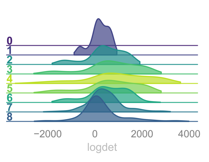
((a)) 100 train steps

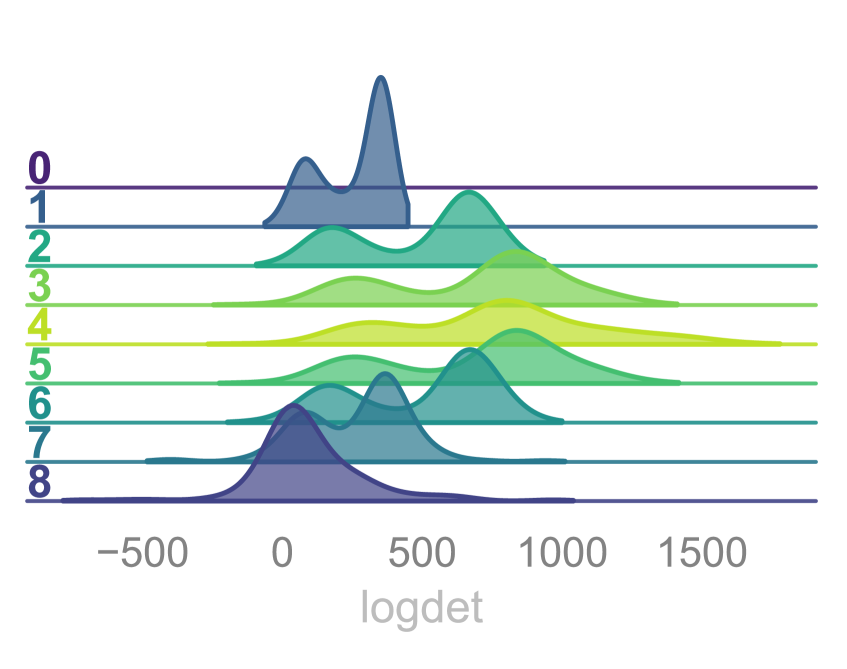
((b)) 500 train steps

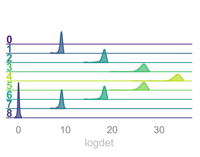
((c)) 1000 train steps

Figure 5: Evolution of $\left|\mathcal{J}\right|$ during the first 1000 training iterations for the 4D $SU(3)$ model.

4 Conclusion

In this work we’ve introduced a generalized MD update for generating 4D $SU(3)$ gauge configurations that can be trained to improve sampling efficiency. Note that this is a relatively simple proof of concept demonstrating how to construct such a sampler. In a future work we plan to further investigate (and quantify) the cost / benefit when compared to alternative approaches such as traditional HMC and purely generative (OT / KL-Divergence [2, 3, 4, 15]) based approaches.

5 Acknowledgements

This research used resources of the Argonne Leadership Computing Facility, which is a DOE Office of Science User Facility supported under Contract DE-AC02-06CH11357. This research was supported by the Exascale Computing Project (17-SC-20-SC), a collaborative effort of the U.S. Department of Energy Office of Science and the National Nuclear Security Administration.

Appendix A Appendix

A.1 Force Term

We can write the force term as

$$F=-\frac{1}{\lambda^{2}}\sum_{k}\lambda^{k}\,\mathrm{Tr}\left[i\left(UA-A^{\dagger}U^{\dagger}\right)\lambda^{k}\right]$$ (38)

where $A$ is the sum over staples

$$A=\sum_{\mu\neq\nu} U_{\mu}(x+\hat{\mu})\,U^{\dagger}_{\mu}(x+\hat{\nu})\,U^{\dagger}_{\nu}(x)$$ (39)

$$+\sum_{\mu\neq\nu}U_{-\nu}(x+\hat{\mu})\,U^{\dagger}_{\mu}(x-\hat{\nu})\,U^{\dagger}_{-\nu}(x).$$ (40)

Since, $i\left(UA-A^{\dagger}U^{\dagger}\right)\in\mathfrak{su}(3)$, we can write it in terms of the generators $\lambda^{k}$ as

$$\sum_{k}\lambda^{k}\,\mathrm{Tr}\left[\lambda^{k}\sum_{j}c_{j}\,\lambda^{j}\right] =\sum_{k}\sum_{j}c_{j}\,\lambda^{j}\,\mathrm{Tr}\left[\lambda^{k}\,\lambda^{j}\right]$$ (41)

$$=\frac{1}{2}\sum_{k}\sum_{j}c_{j}\,t^{k}\,\delta_{jk}$$ (42)

$$=\frac{1}{2}\sum_{k}c_{k}\,t^{k}$$ (43)

consequently, we can simplify the force term as

$$F[U]=-\frac{1}{2g^{2}}\,i\,\left(UA-A^{\dagger}U^{\dagger}\right).$$ (44)

A.2 Topological Charge $Q$

In lattice field theory, the topological charge $Q$ is defined as the 4D integral over spacetime of the topological charge density $q$. In the continuum,

$$Q =\int d^{4}xq(x),\text{ where }$$ (45)

$$q(x) =\frac{1}{32\pi^{2}}\epsilon_{\mu\nu\rho\lambda}\mathrm{Tr}\left\{F_{\mu\nu}F_{\rho\lambda}\right\}$$ (46)

On the lattice, we choose a discretization $q_{L}(x)$ such that $Q=a^{4}\sum_{x}q_{L}(x)$. The most obvious discretization of $q_{L}$ uses the $1\times 1$ plaquette $P_{\mu\nu}(x)$, and can be written as

$$q^{\mathrm{plaq}}_{L}(x)=\frac{1}{32\pi^{2}}\epsilon_{\mu\nu\rho\lambda}\mathrm{Tr}\left\{P_{\mu\nu}(x)P_{\rho\lambda}(x)\right\}$$ (47)

this has the advantage of being computationally inexpensive, but leads to lattice artifacts of order $\mathcal{O}(a^{2})$.

References

- [1] M. Abadi, A. Agarwal, P. Barham, E. Brevdo, Z. Chen, C. Citro, G. S. Corrado, A. Davis, J. Dean, M. Devin, S. Ghemawat, I. Goodfellow, A. Harp, G. Irving, M. Isard, Y. Jia, R. Jozefowicz, L. Kaiser, M. Kudlur, J. Levenberg, D. Mane, R. Monga, S. Moore, D. Murray, C. Olah, M. Schuster, J. Shlens, B. Steiner, I. Sutskever, K. Talwar, P. Tucker, V. Vanhoucke, V. Vasudevan, F. Viegas, O. Vinyals, P. Warden, M. Wattenberg, M. Wicke, Y. Yu, and X. Zheng. TensorFlow: Large-scale machine learning on heterogeneous distributed systems. URL http://arxiv.org/abs/1603.04467.
- Albergo et al. [a] M. Albergo, G. Kanwar, and P. Shanahan. Flow-based generative models for markov chain monte carlo in lattice field theory. 100(3):034515, a. ISSN 2470-0010, 2470-0029. doi: 10.1103/PhysRevD.100.034515. URL https://link.aps.org/doi/10.1103/PhysRevD.100.034515.
- Albergo et al. [b] M. S. Albergo, D. Boyda, D. C. Hackett, G. Kanwar, K. Cranmer, S. Racanière, D. J. Rezende, and P. E. Shanahan. Introduction to normalizing flows for lattice field theory, b. URL http://arxiv.org/abs/2101.08176.
- [4] D. Boyda, G. Kanwar, S. Racanière, D. J. Rezende, M. S. Albergo, K. Cranmer, D. C. Hackett, and P. E. Shanahan. Sampling using $SU(n)$ gauge equivariant flows. 103(7):074504. ISSN 2470-0010, 2470-0029. doi: 10.1103/PhysRevD.103.074504. URL http://arxiv.org/abs/2008.05456.
- [5] G. Cossu, P. Boyle, N. Christ, C. Jung, A. Jüttner, and F. Sanfilippo. Testing algorithms for critical slowing down. 175:02008. ISSN 2100-014X. doi: 10.1051/epjconf/201817502008. URL http://arxiv.org/abs/1710.07036.
- [6] L. Dinh, J. Sohl-Dickstein, and S. Bengio. Density estimation using real NVP. URL http://arxiv.org/abs/1605.08803.
- [7] M. Favoni, A. Ipp, D. I. Müller, and D. Schuh. Lattice gauge equivariant convolutional neural networks. 128(3):032003. ISSN 0031-9007, 1079-7114. doi: 10.1103/PhysRevLett.128.032003. URL http://arxiv.org/abs/2012.12901.
- Foreman et al. [a] S. Foreman, X.-Y. Jin, and J. C. Osborn. Deep learning hamiltonian monte carlo, a. URL http://arxiv.org/abs/2105.03418.
- Foreman et al. [b] S. Foreman, X.-Y. Jin, and J. C. Osborn. LeapfrogLayers: A trainable framework for effective topological sampling, b. URL http://arxiv.org/abs/2112.01582.
- [10] S. A. Foreman. Learning better physics: a machine learning approach to lattice gauge theory. URL https://iro.uiowa.edu/esploro/outputs/doctoral/9983776792002771.
- [11] A. Gelman and C. Pasarica. Adaptively scaling the metropolis algorithm using expected squared jumped distance. ISSN 1556-5068. doi: 10.2139/ssrn.1010403. URL http://www.ssrn.com/abstract=1010403.
- [12] W. K. Hastings. Monte carlo sampling methods using markov chains and their applications. 57(1):97–109. ISSN 1464-3510, 0006-3444. doi: 10.1093/biomet/57.1.97. URL https://academic.oup.com/biomet/article/57/1/97/284580.
- [13] M. Hoffman, P. Sountsov, J. V. Dillon, I. Langmore, D. Tran, and S. Vasudevan. NeuTra-lizing bad geometry in hamiltonian monte carlo using neural transport. URL http://arxiv.org/abs/1903.03704.
- [14] J. D. Hunter. Matplotlib: A 2d graphics environment. 9(3):90–95. ISSN 1521-9615. doi: 10.1109/MCSE.2007.55. URL http://ieeexplore.ieee.org/document/4160265/.
- [15] G. Kanwar, M. S. Albergo, D. Boyda, K. Cranmer, D. C. Hackett, S. Racanière, D. J. Rezende, and P. E. Shanahan. Equivariant flow-based sampling for lattice gauge theory. 125(12):121601. ISSN 0031-9007, 1079-7114. doi: 10.1103/PhysRevLett.125.121601. URL https://link.aps.org/doi/10.1103/PhysRevLett.125.121601.
- [16] R. Kumar, C. Carroll, A. Hartikainen, and O. Martin. ArviZ a unified library for exploratory analysis of bayesian models in python. 4(33):1143. ISSN 2475-9066. doi: 10.21105/joss.01143. URL http://joss.theoj.org/papers/10.21105/joss.01143.
- [17] D. Levy, M. D. Hoffman, and J. Sohl-Dickstein. Generalizing hamiltonian monte carlo with neural networks. URL http://arxiv.org/abs/1711.09268.
- [18] Z. Li, Y. Chen, and F. T. Sommer. A neural network MCMC sampler that maximizes proposal entropy. URL http://arxiv.org/abs/2010.03587.
- [19] M. Medvidovic, J. Carrasquilla, L. E. Hayward, and B. Kulchytskyy. Generative models for sampling of lattice field theories. URL http://arxiv.org/abs/2012.01442.
- [20] Y. Nagai and A. Tomiya. Gauge covariant neural network for 4 dimensional non-abelian gauge theory. URL http://arxiv.org/abs/2103.11965.
- [21] K. Neklyudov and M. Welling. Orbital MCMC. URL http://arxiv.org/abs/2010.08047.
- [22] K. Neklyudov, M. Welling, E. Egorov, and D. Vetrov. Involutive MCMC: a unifying framework. URL http://arxiv.org/abs/2006.16653.
- [23] F. Perez and B. E. Granger. IPython: A system for interactive scientific computing. 9(3):21–29. ISSN 1521-9615. doi: 10.1109/MCSE.2007.53. URL http://ieeexplore.ieee.org/document/4160251/.
- [24] D. J. Rezende, G. Papamakarios, S. Racanière, M. S. Albergo, G. Kanwar, P. E. Shanahan, and K. Cranmer. Normalizing flows on tori and spheres. URL http://arxiv.org/abs/2002.02428.
- [25] C. P. Robert. The metropolis-hastings algorithm. URL http://arxiv.org/abs/1504.01896.
- [26] S. Schaefer, R. Sommer, and F. Virotta. Investigating the critical slowing down of QCD simulations. In Proceedings of The XXVII International Symposium on Lattice Field Theory — PoS(LAT2009), page 032. Sissa Medialab. doi: 10.22323/1.091.0032. URL https://pos.sissa.it/091/032.
- [27] A. Sergeev and M. Del Balso. Horovod: fast and easy distributed deep learning in TensorFlow. URL http://arxiv.org/abs/1802.05799.
- [28] A. Tanaka and A. Tomiya. Towards reduction of autocorrelation in HMC by machine learning. URL http://arxiv.org/abs/1712.03893.
- [29] M. Waskom, O. Botvinnik, D. O’Kane, P. Hobson, S. Lukauskas, D. C. Gemperline, T. Augspurger, Y. Halchenko, J. B. Cole, J. Warmenhoven, J. De Ruiter, C. Pye, S. Hoyer, J. Vanderplas, S. Villalba, G. Kunter, E. Quintero, P. Bachant, M. Martin, K. Meyer, A. Miles, Y. Ram, T. Yarkoni, M. L. Williams, C. Evans, C. Fitzgerald, Brian, C. Fonnesbeck, A. Lee, and A. Qalieh. mwaskom/seaborn: v0.8.1 (september 2017). URL https://zenodo.org/record/883859.
- [30] A. Wehenkel and G. Louppe. You say normalizing flows i see bayesian networks. URL http://arxiv.org/abs/2006.00866.