Limit Order Book Dynamics and Order Size Modelling Using Compound Hawkes Process

Abstract.

Hawkes Process has been used to model Limit Order Book (LOB) dynamics in several ways in the literature however the focus has been limited to capturing the inter-event times while the order size is usually assumed to be constant. We propose a novel methodology of using Compound Hawkes Process for the LOB where each event has an order size sampled from a calibrated distribution. The process is formulated in a novel way such that the spread of the process always remains positive. Further, we condition the model parameters on time of day to support empirical observations. We make use of an enhanced non-parametric method to calibrate the Hawkes kernels and allow for inhibitory cross-excitation kernels. We showcase the results and quality of fits for an equity stock’s LOB in the NASDAQ exchange.

1. Introduction

The Hawkes process, known for its high adaptability, offers a more comprehensive point process methodology for modeling order book arrivals than the Poisson process and its variants, without the need to explicitly model individual traders’ behaviors in the market. Its capability to replicate microstructural details such as volatility clustering and correlated order flow makes it a suitable candidate for Limit Order Book (LOB) models. It is important to highlight that these point process models are mathematically descriptive, providing full transparency in their nature and thus are suitable for applications where black-box solutions are not preferred. In their comprehensive review and tutorial, Bacry et al. (Bacry et al., 2015) outlay the major ideas of the Hawkes Process, its mathematical theory, some of its crucial properties and finally applications including a detailed review over the Order Book models. Recently, state dependent Hawkes Process have been quite popular ((Morariu-Patrichi and Pakkanen, 2022), (Kirchner and Vetter, 2022), (Mucciante and Sancetta, 2023), (Wu et al., 2019)). However, as noted in (Rambaldi et al., 2017) and (Lu and Abergel, 2018b), individual order’s size is an important of aspect of the LOB which the Hawkes model alone is unable to capture.

1.1. Empirical Distributions of Order Sizes:

We show here in Figure 1 two trading weeks’ of data (10 dates) for Apple and plot the empirical histograms on a log-log scale. We only focus on top of the book cancels and limit orders. As Figures 1(a) and 1(b) show, the market orders and limit orders sizes have several spikes at round numbers indicating the preference of the traders. For example, we see more than 40% of the market orders and 60% of limit orders are of 100 size. Naturally, Cancel Orders’ sizes are capped at the size of an individual order. In fact we observe that outright cancels (i.e. full quantity of an order is cancelled) constitute 99.3% of all cancels.

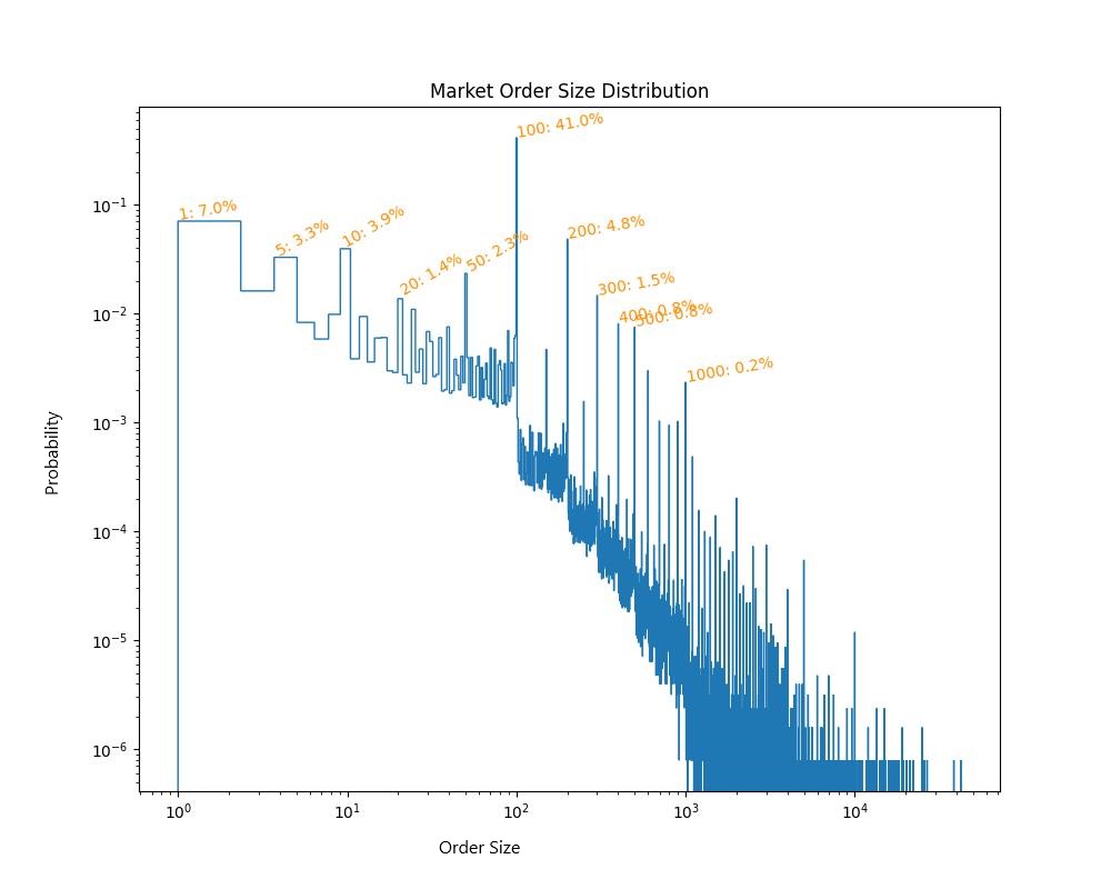
(a) Market Orders’ Size Distribution (log-log scale)

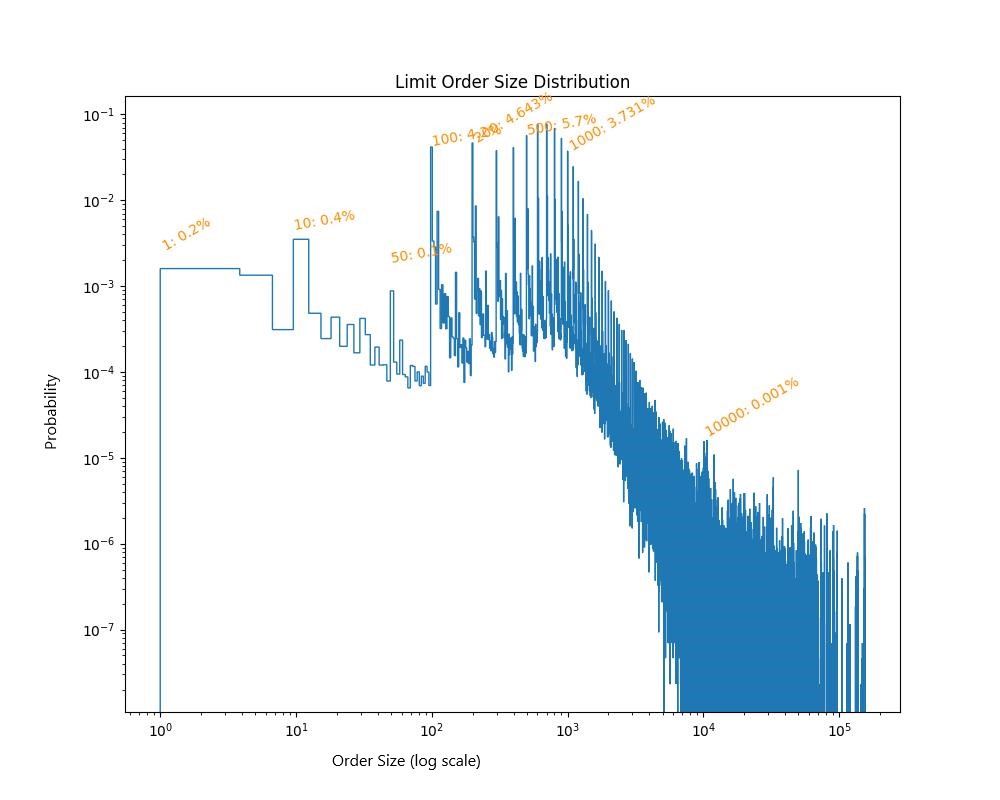
(b) Limit Orders’ Size Distribution (log-log scale)

Figure 1. Empirical Distribution of Order Sizes

1.2. Properties of the Order Book Dynamics:

There have been several variations to the Hawkes model to accommodate for certain properties of the order book in exchanges.

Prop 1: Bid-Ask Spread is always non-negative: The bid-ask spread can never be less than zero being an important one was tackled by using order arrival intensities dependent on spread-in-ticks by (Lee and Seo, 2022). Previously, Zheng et al. (Zheng et al., 2014) have used constrained Hawkes Process to control negative spreads.

Prop 2: Order intensities are dependent on time-of-day: It is well known that trading volumes follow an intraday seasonality which is observered to be stationary across multiple days. Naturally, we observe that the order intensities too exhibit this intraday seasonality (more in Section 2). Hawkes models have been adapted to account for the same in (Mucciante and Sancetta, 2023), (Prenzel et al., 2022), and (Kirchner and Vetter, 2022).

Prop 3: Cross-excitations can be inhibitory: As noted in (Lu and Abergel, 2018a), the cross-excitation of events need not necessarily always be catalyzing. For example, we observe that limit orders inside the spread and cancels at top at opposing sides of the book have inhibitory effects on each other. Generally modelling for this can introduce negative intensities in the point process. To avoid such complications, Lu et al. (Lu and Abergel, 2018a) propose to floor the total intensity of any element of the Hawkes process to zero.

In this work we show some lack of support for the hypothesis that the order arrival intensities are impacted by the past order sizes. Thus we conclude that the Compound Hawkes Process is a suitable candidate for the model. We then create a stationary distribution of the order sizes for each type of order which closely mimics the empirical distribution. This distribution is used to sample the order sizes in the compound Hawkes Process. We create a novel formulation of the Hawkes intensities which satisfies Properties 1, 2 and 3. In Section 3, we show the calibration results for the Apple Inc. stock by using Level 2 data in the NASDAQ exchange. We also provide an analysis for the quality of fit.

2. Methodology

We consider the task of modelling LOB’s current best bid and ask (i.e. Level 1 LOB). We note that since placing order in the spread is a common practice in equities, the reason being that the spread usually has many empty price levels to attract market participants to place a more aggressive order, the Hawkes formulation should contain modelling the intensity of the nearby empty levels as well. Hence we formulate the order book as a queueing system with six different queues which are $\{\text{ask}_{+1},\text{ask}_{0},\text{ask}_{-1},\text{bid}_{+1},\text{bid}_{0},\text{bid}_{-1}\}$.

Figure 2. Order Book Snapshot

Here $\text{ask}_{0}$ and $\text{bid}_{0}$ are the respective best ask and bid prices while the subscripts denote the price level distance in ticks from the best ask/bid. For eg. $\text{ask}_{+1}$ is the price level which is 1 tick more than $\text{ask}_{0}$. The $2\times 6$ vector of $((q^{(s)}_{k},s_{k})_{s\in\{\text{ask},\text{bid}\},k\in\{-1,0,+1\}})$, where $q^{(s)}_{k}$ denotes the queue size, is what we define as the state of the order book. The motivation to model just these six levels and not the entire order book is two-fold. Firstly, the question of parsimony becomes important when we model more levels than just these six. Secondly, we observe that the LOB state changes are generally events which move the prices by 1 tick. Indeed we observe, in our dataset, 97.4% of all in-spread orders occur 1-tick away from the best respective quote with mean being $1.035\pm 0.285$ ticks for 2 million samples, and 97.5% of all price changes have the next non-empty price level at 1-tick distance as well with the mean being $1.033\pm 0.283$ ticks.

Mechanical Constraints: Naturally, since $\text{ask}_{0}$ and $\text{bid}_{0}$ are the best ask and bid prices, the queue size at $\text{ask}_{-1}/\text{bid}_{+1}$ is zero. Therefore any incoming limit order at $\text{ask}_{-1}/\text{bid}_{+1}$ (i.e. an in-spread (IS) order) creates a new best ask/bid and so the LOB state transforms from

$$S:=\{ (q^{(\text{ask})}_{+1},\text{ask}_{+1}),(q^{(\text{ask})}_{0},\text{ask}_{0}),(0,\text{ask}_{-1}),$$

$$(0,\text{bid}_{+1}),(q^{(\text{bid})}_{0},\text{bid}_{0}),(q^{(\text{bid})}_{-1},\text{bid}_{-1})\}$$

to

$$S_{IS}=\{ (q^{(\text{ask})}_{0},\text{ask}_{0}),(q^{(\text{ask})}_{-1},\text{ask}_{-1}),(0,\text{ask}_{-2}),$$

$$(0,\text{bid}_{+1}),(q^{(\text{bid})}_{0},\text{bid}_{0}),(q^{(\text{bid})}_{-1},\text{bid}_{-1})\}$$

for an in-spread ask side limit order.

Note that it is possible that the spread is only 1-tick wide which would mean $\text{ask}_{-1}$ and $\text{bid}_{+1}$ coincides. There is also the possibility of zero spread in which case $\text{ask}_{-1}$ and $\text{bid}_{+1}$ do not exist. We will put some constraints on the Hawkes process intensities for these levels further in this section to account for these possibilities. On the other hand, if a queue-depletion (QD) event at best bid/ask happens (for eg, a large enough market order), the spread widens and therefore the state moves from $S$ to

$$S_{QD}=\{ (q^{(\text{ask})}_{+2},\text{ask}_{+2}),(q^{(\text{ask})}_{+1},\text{ask}_{+1}),(0,\text{ask}_{0}),$$

$$(0,\text{bid}_{+1}),(q^{(\text{bid})}_{0},\text{bid}_{0}),(q^{(\text{bid})}_{-1},\text{bid}_{-1})\}$$

for a queue-depleting ask side market order/cancel order. Here we observe an unknown quantity $q^{(\text{ask})}_{+2}$. We sample this unknown quantity from a stationary distribution calibrated from empirical data. Finally, we note that Market Orders can only occur at $\text{ask}_{0}/\text{bid}_{0}$ and $\text{ask}_{-1}/\text{bid}_{+1}$ cannot have Cancel Orders since by definition the quantity there is zero.

Compound Hawkes Process: A compound point process (CPP) $Z_{t}$ is defined as

(1) $$Z_{t}=\sum^{N(t)}_{i=1}Y_{i}$$

where $\{N(t):t\geq 0\}$ is the counting process associated with a point process $\{Y(t):t\geq 0\}$ with intensity $\lambda(t)$, and $Y_{i}\sim P_{\Theta}(Y_{i})$ is a random variable denoting the jump size with the corresponding $P_{\Theta}(Y_{i})$ being the jump size distribution. Compound Hawkes process (CHP) is a special case of the CPP where $N(t)$ is a counting process associated with a Hawkes Process. For a $d$-dimensional Hawkes process the intensity of the process $\lambda^{(i)}_{t}$ and the associated counting process $N^{(i)}_{t}$ for $i=1,\ldots,d$ is defined as:

(2) $$\lambda^{(i)}_{t}=\mu^{(i)}_{t}+\sum^{d}_{j=1}\sum_{t_{j}\in T_{j}}\phi^{(j\rightarrow i)}(t-t_{j})$$

where $T_{j}:=\{t_{j}:t_{j}\leq t\}$ denotes the set of past event times in the $j$ dimension of the Hawkes Process. Here, $\mu^{(i)}_{t}$ is the exogenous intensity of the $i$-th dimension and $\phi^{(j\rightarrow i)}(t-t_{j})$ is the excitation term from $j$-th dimension to $i$-th dimension. The excitation terms are a function of the time since the event (generally a decaying function in time like exponential decay or power law decay). An alternate but similar formulation is the following:

(3) $$\lambda^{(i)}_{t}=\mu^{(i)}_{t}+\sum^{d}_{j=1}\int^{t}_{0}\phi^{(j\rightarrow i)}(t-s)dN^{(j)}_{s}$$

Limit Order Book at Compound Hawkes Process: We define a 12D Compound Hawkes Process (in accordance with the mechanical constraints) for the 6 queues in the order book state where each dimension corresponds to the following event types:

$$\{LO_{\text{ask}_{+1}},CO_{\text{ask}_{+1}},LO_{\text{ask}_{0}},CO_{\text{ask}_{0}},MO_{\text{ask}_{0}},LO_{\text{ask}_{-1}},$$

$$LO_{\text{bid}_{+1}},LO_{\text{bid}_{0}},CO_{\text{bid}_{0}},MO_{\text{bid}_{0}},LO_{\text{bid}_{-1}},CO_{\text{bid}_{-1}}\}$$

where LO is Limit Order, CO is Cancel Order and MO is Market Order. Here each of the 12 event types’ order size ($\kappa^{(e)}$ for event $e$) is sample from their own specific calibrated distribution ($\Pi^{(e)}(\Theta)$). We postulate that the order intensities themselves are not impacted by the past order sizes but only the past order event-times as is the general assumption in Hawkes models applied to LOB data. We provide some weak evidence for this claim in the Appendix A. We note that our work on the distribution of order size closely follows the work by Lu et al. (Lu and Abergel, 2018b) however they make use of a Poisson model. Let us also mention that Abergel et al. (Abergel et al., 2016) too use parametric distributions for order sizes in the Hawkes Process model. For Cancel Order quantities, since we observe almost all cancels in empirical data are outright cancels, we draw randomly, with equal probability, from the available limit orders’ quantities in the queue. We thus create a CHP for the queue-sizes at the six queues of the LOB:

(4) $$q^{(s)}_{k}(t) =\sum_{e\in E^{(s)}_{k}}\sum^{N^{(e)}(t)}_{i}\kappa^{(e)}_{i}$$

(5) $$\kappa^{(e)}_{i} \sim\Pi^{(e)}(\Theta)$$

where $i=1,\ldots,N^{(e)}(t)$ and $E^{(s)}_{k}\text{is the set of eligible events for $s$ and $k$}$

To control the spread of the process (Prop 1), we formulate the intensities of $LO_{\text{ask}_{-1}}$ and $LO_{\text{bid}_{+1}}$ in the following manner as a function of the current spread-in-ticks ($s$). If $\psi^{(.)}_{t}$ represents the intensity (either exogenous or excitation), then,

(6) $$\psi^{(.)}_{t}(s)=(\psi^{(.)}_{t})s^{\beta};\beta>0,s\in\mathbb{N}$$

In this formulation we enforce the mechanical constraint if $s=0$, $\lambda^{LO_{\text{ask}_{-1}}}_{t}=\lambda^{LO_{\text{bid}_{+1}}}_{t}=0$ with an extra parameter $\beta$. We motivate the choice of a power law dependence of order intensity over spread in Appendix B.

We observe a strong dependence between the intensities $\lambda^{(.)}_{t}$ on the time of day of the trading day (Prop 2). There is a ”U”-shape of order intensities with respect to the time of day i.e. right after the open auction and before the close auction, the activity in the market is much higher than the middle of the day. This effect is observed for trading volumes in equities with a number of probable causes but the most commonly accepted one is that because auctions cause a halt in trading, this halt leads to increased activity. To maintain model parsimony, we bin the 6.5 hour trading day of NASDAQ into thirteen 30-minute bins (indexed by $Q_{t}\in\{1,2,...,13\}$) for $t$ being a time of day). We model the intensity as a separable function of time-of-day and the Hawkes Intensities:

(7) $$\lambda^{(i)}(Q_{t},t,s)=f(Q_{t})\times\lambda^{(i)}(t,s)$$

Finally, to make sure the inhibitory kernels do not create negative intensities, we floor the total excitation $\lambda^{(i)}(Q_{t},t,s)$ to zero.

Price Dynamics: The mid price ($P(t)$) dynamics after an event at $t$ at side $\zeta$ (and $\xi$ = +1 for $\zeta=$ ask and -1 for $\zeta=$ bid) is a jump process with jumps defined by :

$$P\left(t^{+}\right)-P(t)= -\frac{\eta}{2}\xi dN^{(IS)}(t)$$

$$+\frac{\eta}{2}\xi dN^{(CO)}(t)\mathbb{1}_{\{\#q_{0}^{(\zeta)}(t)=1\}}(t)$$

(8) $$+\frac{\eta}{2}\xi dN^{(MO)}(t)\mathbb{1}_{\{q^{(\zeta)}_{0}(t)\leq\kappa^{(MO_{\zeta_{0}})}(t)\}}(t)$$

where $\eta$ is the tick-size, $N^{(IS)}(t)$ is the counting process for IS orders, and $\#q_{0}^{(\zeta)}(t)$ denotes the number of individual limit orders in the queue.

Calibration: We follow the non-parametric method of calibration in (Kirchner, 2017) and take inspiration from (Bacry et al., 2016) to create a time grid at both linear and log scales to account for the slowness of the decay kernels. This method has the advantage of not having any priors on the shape of the kernels themselves (popular choices in the literature include exponential decay and power-law decay) since it is non-parametric. We fit parametric functions on each of these kernels on these point estimates and here we make use of power-law functions and exponential functions as the candidates. Unlike (Kirchner, 2017), however, we do not calibrate the parameters in 30-minute windows and average over a day’s 13 windows, but rather we use the entire day’s data to calibrate the parameters. We also modify the calibration methodology to account for the time-of-day dependence of the intensities as well as the spread dependent formulation we developed for in-spread queues. We add two constraints to the least squares problem (from the auto-regressive formulation of (Kirchner, 2017)). Firstly, we enforce the unidirectional shape of the Hawkes Kernels by constraining the point estimates to be uniform in sign (i.e., either all greater than 0 or all less than 0). Secondly, we constrain the integral of a Hawkes Kernel to be less than 1 to ensure the stability of the Hawkes Process. For the first constraint, we make use of the Hawkes Graph (Achab et al., 2018) which directly estimates the kernel norms matrix : $\boldsymbol{M}_{d\times d}$ (elements of which are defined as $M_{ij}=\int_{0}^{\infty}\phi^{j\rightarrow i}(s)ds$ which is the kernel norm of $\phi^{j\rightarrow i}(t)$ for $i,j\in\{1,...,d\}$) from the conditional probabilities of the 12D point process. Note that we purely use this method to identify whether a kernel is catalysing or inhibiting in nature (i.e. is the kernel norm positive or negative). Now for the second constraint, as noted in (Bacry et al., 2015), a Hawkes Process is stable if the maximum eigenvalue of the Kernel Norm matrix is $<1$. We postulate that the above formulation is an adequate linear approximation to the non-linear constraint of bounded eigenvalues. In practice, we do see the calibrated Hawkes Kernel to occasionally violate this non-linear constraint. We apply a heuristic of multiplying all the kernels by a regularizing term to cap the eigenvalue at $1$. We reserve the question of how this heuristic impacts the fit quality for future work.

We calibrate the data for several days individually and test the stationarity (by day) of the calibrated parameters. Since we do see stationarity in the kernel parameters over multiple days (Figure 4(b)), we conclude by using the parameters over multiple days for our final calibrated parameters’ estimation. We use a heuristic method to calibrate the order size distribution. A key observation is the preference of traders of round numbers in their order quantity. This is an important stylized fact of the order book dynamics so we make use of Dirac delta functions to add spikes in the distribution function to account for this. Finally, we use the thinning algorithm to simulate the order book from the calibrated parameters and provide some visualizations of the calibrated parameters in the following section along with the quality of fit results.

3. Results

3.1. Calibration of Hawkes Process:

We now show the observed intensities conditioned by time of day for a sample dimension (Market Orders at Ask) in Figure 3. We observe the common U-shape across all 12 dimensions. In Figure 4(a), we show the the norm of kernels $\boldsymbol{M}$, removing the time-of-day multiplier. The $x$ axis shows the excitor and $y$ axis is the excitee. We also show some sample fitted kernel shapes in Figure 4(b). As we can see here in the translucent blue lines, the kernel shapes fitted over multiple days are stable across days.

Since the number of excitation kernels in a 12D Hawkes Process are 12², in order to maintain model parsimony, we zero-out the effect of small cross-excitations such as Cancel Bid₀ $\rightarrow$ Limit Ask₀. We set the threshold to select kernels on the basis of their norms to 0.01 as it eliminates several cross-excitation terms to limit the number of kernels to 65.

Note that these estimated kernels are estimated in a non-parametric manner and hence need to be further fitted on a parametric function. We choose between the power-law kernel : $\phi(t)=\alpha(1+\gamma t)^{-\beta}$ and the exponential kernel : $\phi(t)=\alpha e^{-\beta t}$ to do the parametric fit by comparing the fit’s Akaike Information Criteria (AIC). We see that the power-law kernel is selected 100% of the time for this dataset. We show the fitted line in 4(b) in red. As we can see, the power law line fits the point estimates quite well. Indeed we see an average mean square fit error to be $\sim 10^{-3}$ . Another noteworthy aspect of the fitting results is the presence of inhibitory kernels.

Figure 3. Intensities conditioned by Time of Day : we report the average number of events per 30 min bin in a 6 month period

3.2. Calibration of Order Size Distributions

Following (Lu and Abergel, 2018a), we use Dirac delta at round numbers to account for the stylized facts we observe in Figure 1(a) and 1(b). We choose the set 1, 10, 50, 100, 200, 500 as the set of round numbers we wish to put spikes in the PDF at. The remainder of the PDF is modelled by a Geometric distribution. We fit this distribution using the maximum likelihood method. We show the final calibrated PDF (smoothened for illustration purposes) in Figure 5.

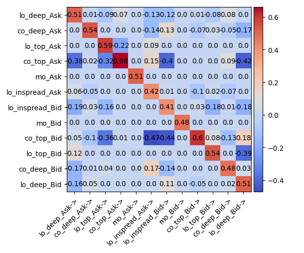
(a) Norms of Kernel

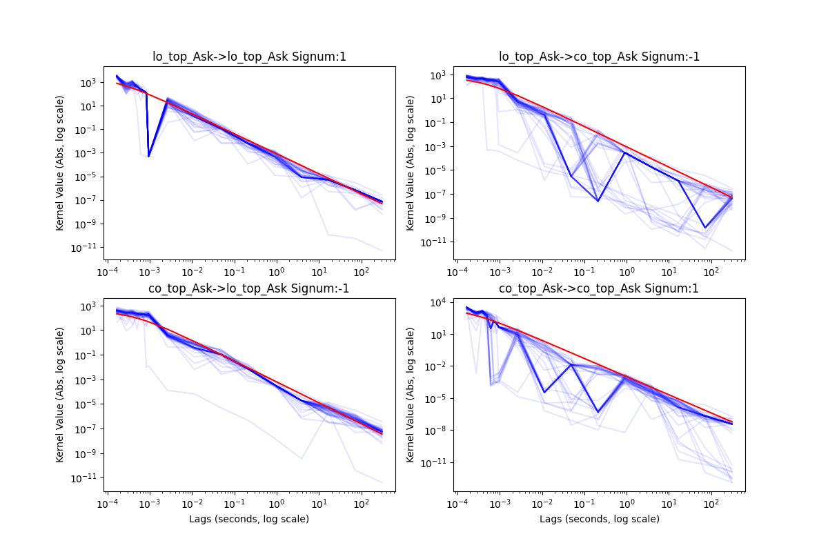
(b) Kernel Shape: non-parametric point estimates (blue) and parametric power-law fit (red) - (log-log scale)

Figure 4. Excitation Kernels

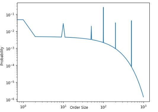
(a) Market Orders’ Size Distribution (log-log scale)

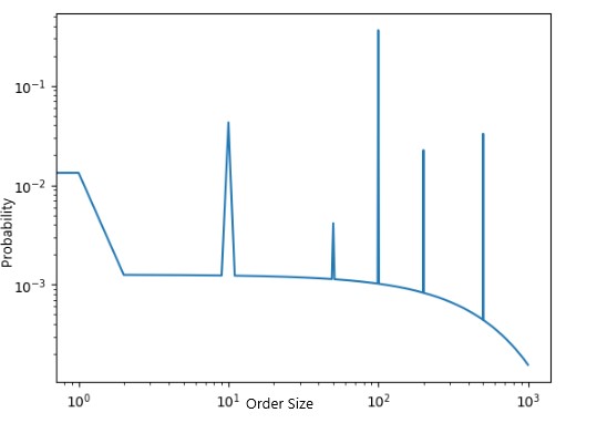
(b) Limit Orders’ Size Distribution (log-log scale)

Figure 5. Fitted Distribution of Order Sizes

3.3. Quality of fit metrics:

We present the quality of fit metrics in Figure 6. We perform a realism quality of fit by comparing some stylized facts of the simulated data to the empirical data. We make use of inter-event durations’ distributions, price change time distributions, signature plots, distribution of spread and returns, autocorrelation of returns and sample price paths as our set of stylized facts.

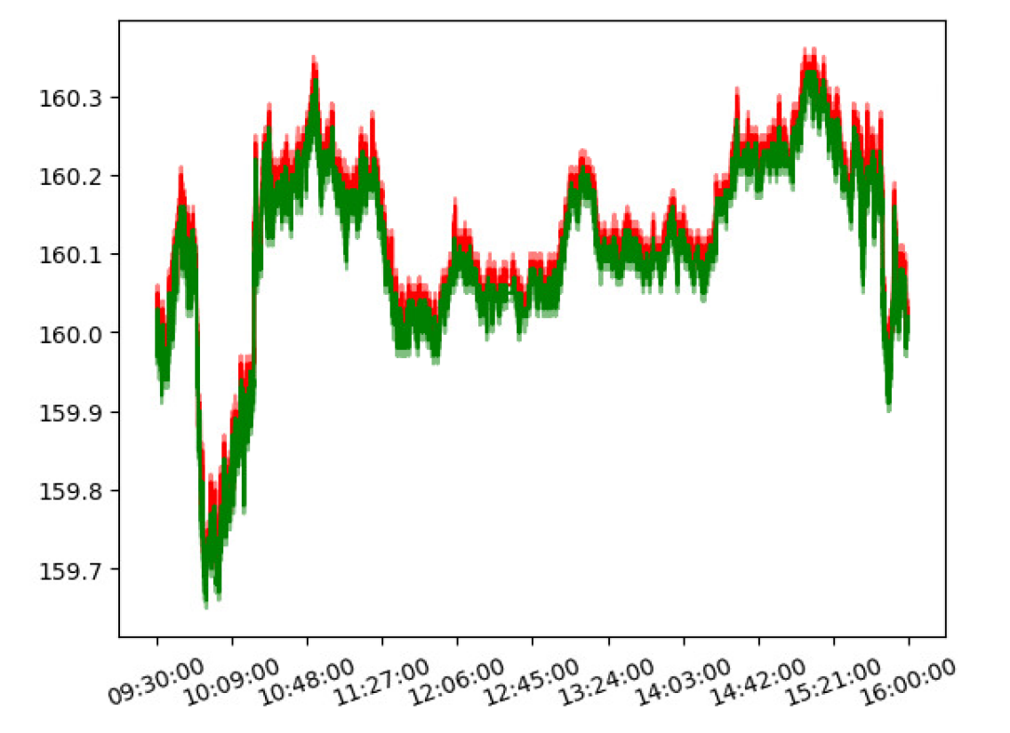
(a) Simulated LOB dynamics

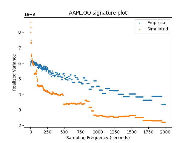
(b) Signature Plot - Simulated vs Empirical

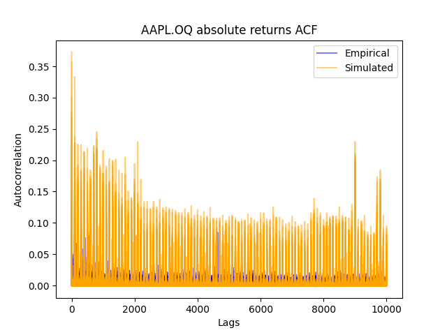
(c) Absolute Returns ACF - Simulated vs Empirical

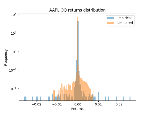
(d) Returns Distribution (log-scale) - Simulated vs Empirical

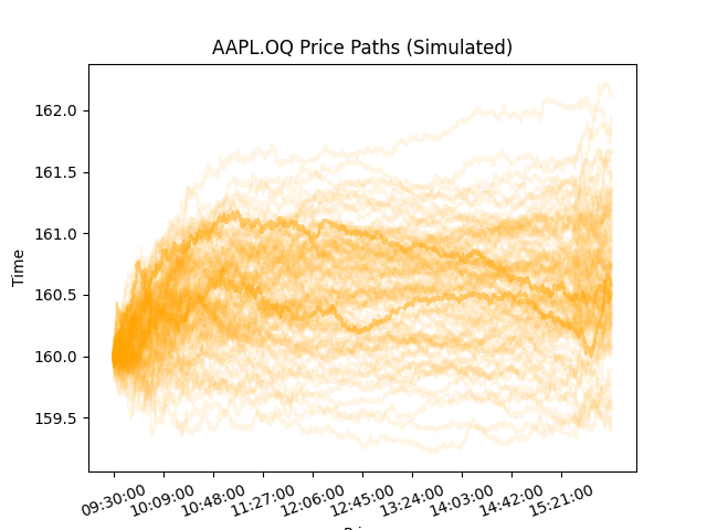
(e) Price Paths - Simulated

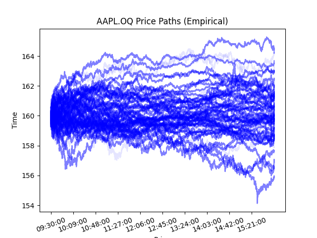
(f) Price Paths - Empirical

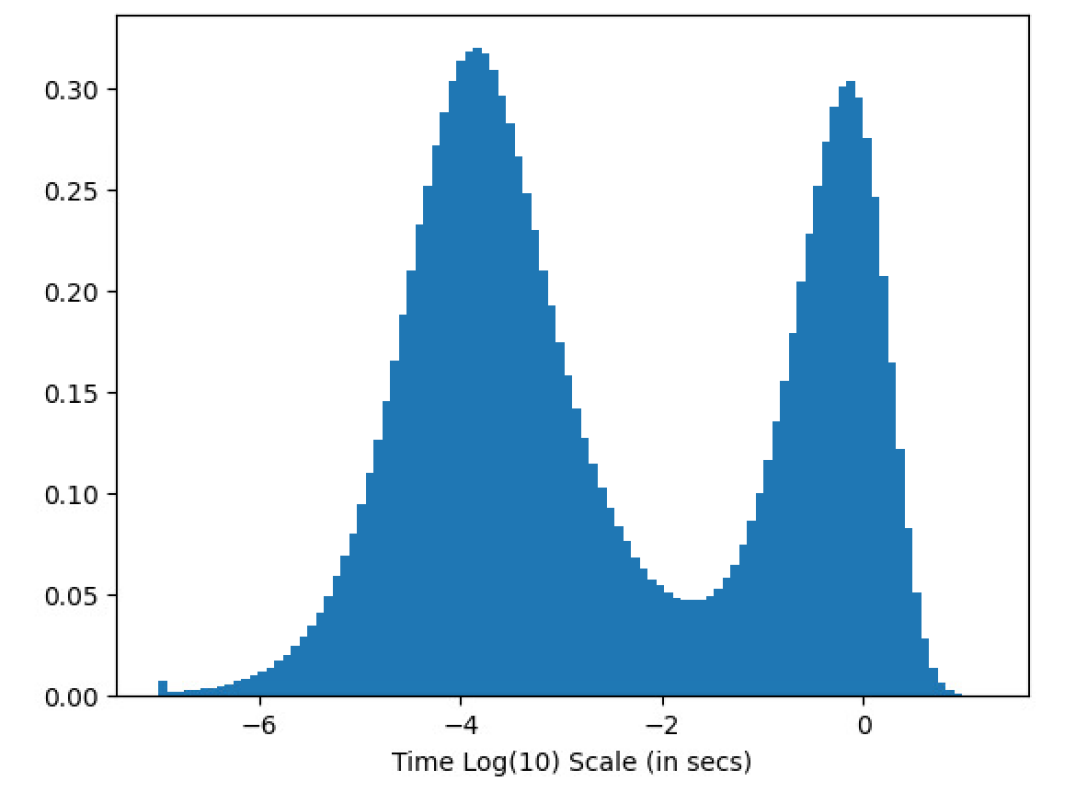
(g) Inter-arrival times - Simulated

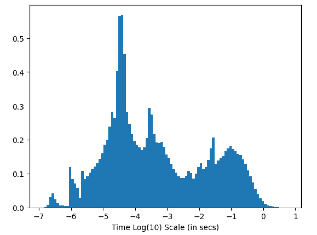
(h) Inter-arrival times - Empirical

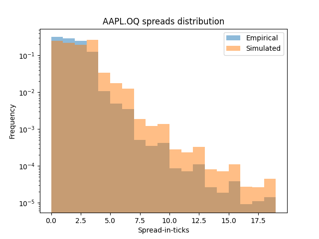
(i) Spread Distribution - Simulated vs Empirical

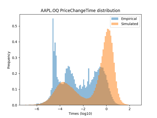
(j) Price Change Time - Simulated vs Empirical

Figure 6. Results

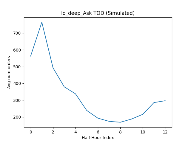
(a) LO(deep, ask)

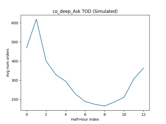
(b) CO(deep, ask)

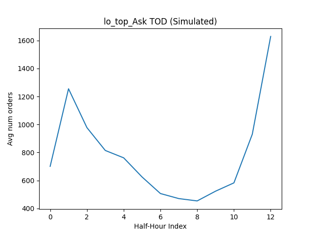
(c) LO(top, ask)

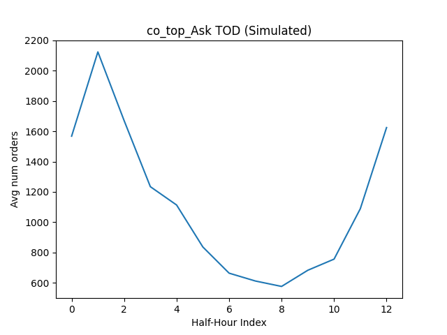
(d) CO(top)

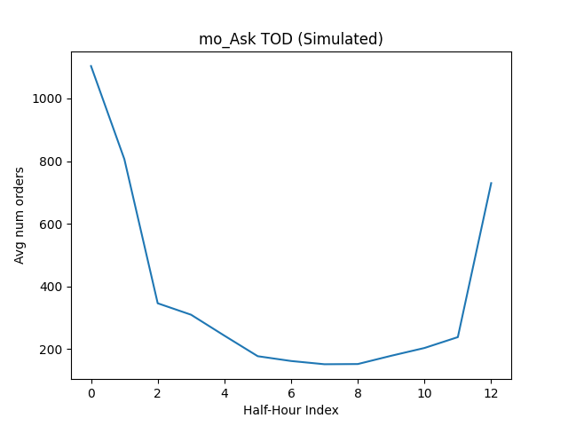
(e) MO(Ask)

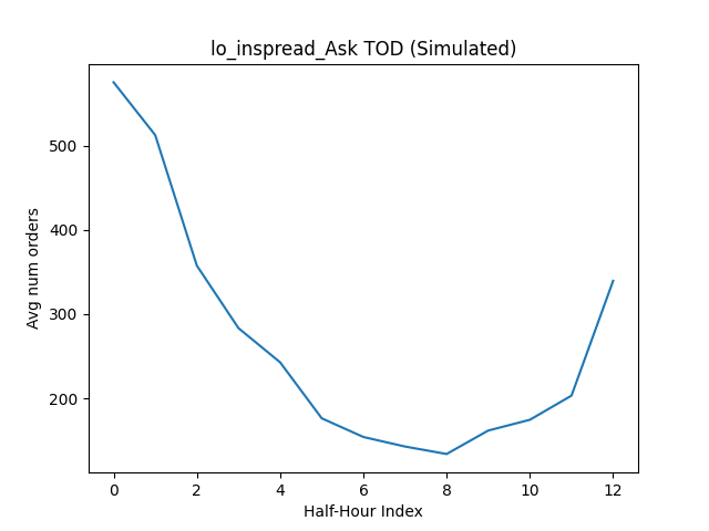
(f) LO(in-spread, Ask)

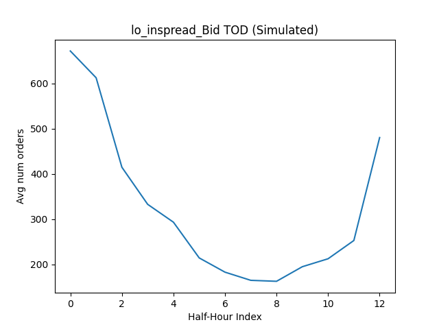
(g) LO(in-spread, Bid)

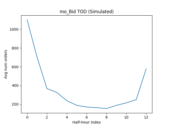
(h) MO(Bid)

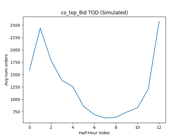
(i) CO(top, Bid)

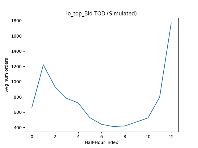
(j) LO(top, Bid)

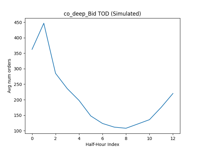
(k) CO(deep, Bid)

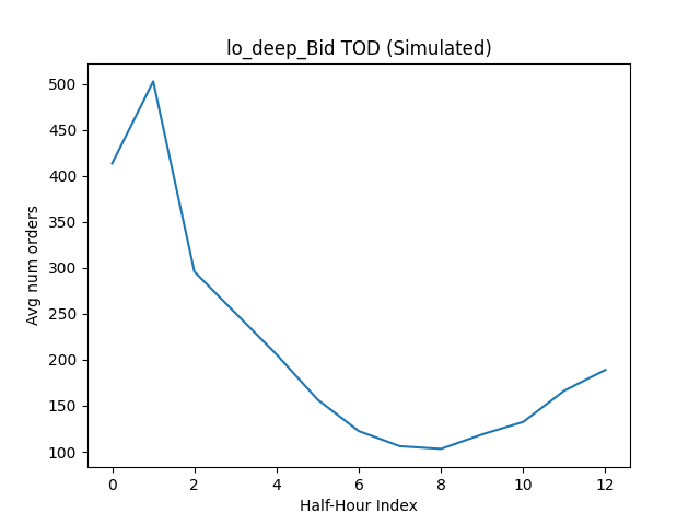
(l) LO(deep, Bid)

Figure 7. Time-of-day shape (simulated)

4. Conclusion & Future Work

We tackle the problem of simulating a realistic order book by using the Compound Hawkes Process. We particularly focus on building a simulator which is realistic in its order sizes and exhibits the mechanical constraints that a real order book has such as non-negative spreads and positive intensities. We further condition the intensities to be dependent on time-of-day in order for the simulator to not be ignorant of the increase in trading intensities around open and close auctions. Finally, we present a number of stylized facts to test the model’s efficacy against empirical observations. As we can see from Figure 6, the Hawkes Process is able to replicate the shape of the Signature Plot, the presence of long auto-correlations of absolute returns, the long tail of returns’ distribution as well as the two peaks in inter-order arrival times quite well. In addition to this, our particular formulation of the Hawkes Process, with its spread control formulation, is able to match the distribution of the empirical spreads quite well. Figure 7 depicts the efficacy of replicating the ”U”-shape dynamics of the order book events in our formulation.

In this formulation of the Hawkes Process, we assume nothing about the Price Process of the equity and rather let it rather emerge as a jump process by modest assumptions about the order flow itself. Our contributions can be enlisted as follows:

1. We propose a novel formulation of the Hawkes Process to maintain positive spread.

2. We augment the non-parameteric methods proposed in (Kirchner, 2017) to work with slow decaying kernels and to be more stable.

3. We make use of calibrated distributions for sampling the order sizes of the events rather than assuming unit order-size.

4. We formulate the in-spread order arrivals as a function of the current spread - utilizing the well known fact that spreads are mean-reverting.

Future directions of research includes testing this model on more equities, particularly tackle the problem of small-tick stocks which have a lower amount of information at the top two levels of the LOB which our model assumes. Though our formulation theoretically can work with small-tick stocks as well but since it limits its modelling to the top of the book, it will be unsuitable for small-tick stocks. We also plan to compare it against the baseline model of a constant order size Hawkes Process model. Further, the number of dimensions of this Hawkes Process is quite high, future research could be focused on simulating the order book with lesser number of dimensions.

5. Disclaimer

Opinions and estimates constitute our judgement as of the date of this Material, are for informational purposes only and are subject to change without notice. This Material is not the product of J.P. Morgan’s Research Department and therefore, has not been prepared in accordance with legal requirements to promote the independence of research, including but not limited to, the prohibition on the dealing ahead of the dissemination of investment research. This Material is not intended as research, a recommendation, advice, offer or solicitation for the purchase or sale of any financial product or service, or to be used in any way for evaluating the merits of participating in any transaction. It is not a research report and is not intended as such. Past performance is not indicative of future results. Please consult your own advisors regarding legal, tax, accounting or any other aspects including suitability implications for your particular circumstances. J.P. Morgan disclaims any responsibility or liability whatsoever for the quality, accuracy or completeness of the information herein, and for any reliance on, or use of this material in any way.

Important disclosures at: www.jpmorgan.com/disclosures

Appendix A Previous Order Sizes do not impact Future Order Arrival Rates

We calculate the next order intensity in our dataset for a past order size by counting the number of future events in a window of $t=0.01$sec. The joint scatter plot for Market Orders at Bid is shown in Figure 8(a). Qualitatively the distribution looks to be quite uniform. We make use of the Hoeffding Independence Test to calculate the distance between the observed joint distribution of these two random variables and the distribution if they were independent. The test statistic is observed to be $0.00068$ which is sufficiently low for us to conclude, albeit with weak evidence, that the two variables are independent. We observe similar scatter plots and Hoeffding statistics for all other events.

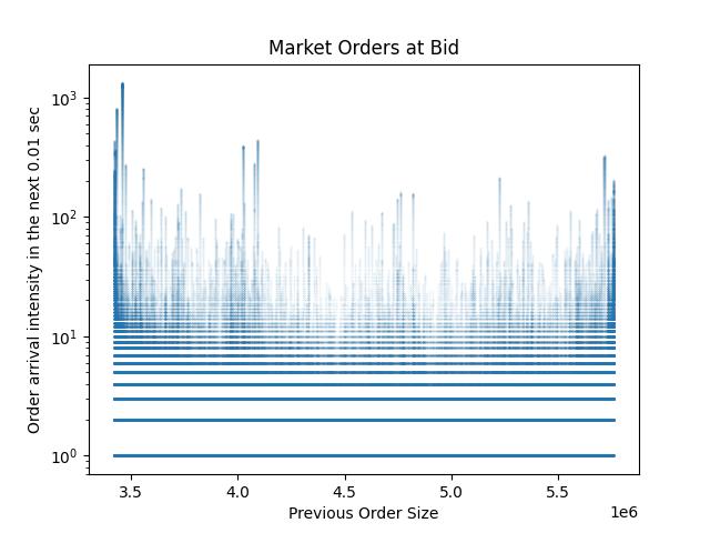
(a) Previous Order Size vs Future Arrival Rates

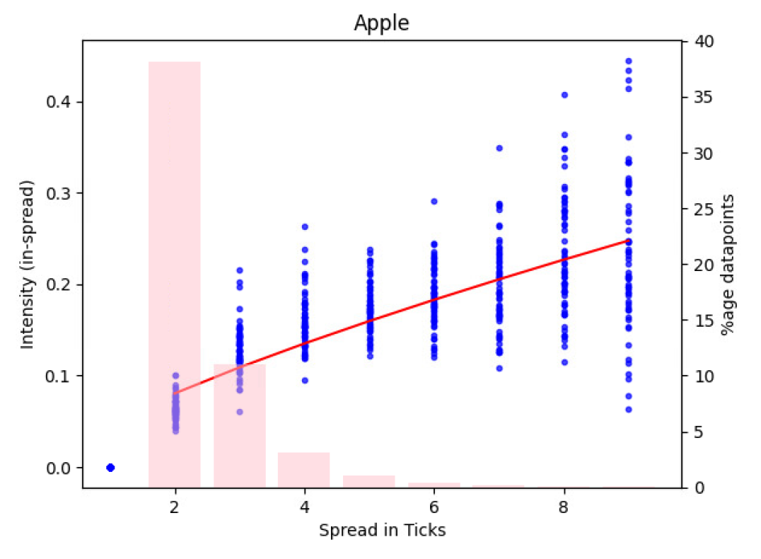
(b) In-Spread Arrival Rates vs Current Spread

Appendix B In-Spread order intensity depends on current spread

We plot the order intensity against the current spread-in-ticks in empirical data (3 months data) in Figure 8(b). Here we show a scatter plot since the intensities are approximated by the number of in-spread orders in the next 0.01 seconds and therefore are random. We show the distribution of data points in the translucent red bars. We fit a linear regressor on log-log transformation of these data points (excluding 0 and 1 spread) and find the best exponent to be $0.7479$. The red line in the plot shows the fitted line. We observe an $R^{2}$ of $0.85$ for this regression.

References

- (1)
- Abergel et al. (2016) Frédéric Abergel, Marouane Anane, Anirban Chakraborti, Aymen Jedidi, and Ioane Muni Toke. 2016. Limit Order Books. Cambridge University Press. https://doi.org/10.1017/CBO9781316683040
- Achab et al. (2018) Massil Achab, Emmanuel Bacry, Stéphane Gaïffas, Iacopo Mastromatteo, and Jean-François Muzy. 2018. Uncovering causality from multivariate Hawkes integrated cumulants. Journal of Machine Learning Research 18, 192 (2018), 1–28.
- Bacry et al. (2015) Emmanuel Bacry, Iacopo Mastromatteo, and Jean-François Muzy. 2015. Hawkes Processes in Finance. Market Microstructure and Liquidity 01, 01 (2015), 1550005. https://doi.org/10.1142/S2382626615500057 arXiv:https://doi.org/10.1142/S2382626615500057
- Bacry et al. (2016) Emmanuel Bacry, Thibault Jaisson, and Jean-François Muzy. 2016. Estimation of slowly decreasing hawkes kernels: application to high-frequency order book dynamics. Quantitative Finance 16, 8 (2016), 1179–1201.
- Kirchner and Vetter (2022) Matthias Kirchner and Silvan Vetter. 2022. Hawkes model specification for limit order books. The European Journal of Finance 28, 7 (2022), 642–662.
- Kirchner (2017) Matthias Kirchner. 2017. An estimation procedure for the Hawkes process. Quantitative Finance 17, 4 (2017), 571–595.
- Lee and Seo (2022) Kyungsub Lee and Byoung Ki Seo. 2022. Modeling Bid and Ask Price Dynamics with an Extended Hawkes Process and Its Empirical Applications for High-Frequency Stock Market Data. Journal of Financial Econometrics (2022), nbab029.
- Lu and Abergel (2018a) Xiaofei Lu and Frédéric Abergel. 2018a. High-dimensional Hawkes processes for limit order books: modelling, empirical analysis and numerical calibration. Quantitative Finance 18, 2 (2018), 249–264. https://doi.org/10.1080/14697688.2017.1403142 arXiv:https://doi.org/10.1080/14697688.2017.1403142
- Lu and Abergel (2018b) Xiaofei Lu and Frédéric Abergel. 2018b. Order-book modeling and market making strategies. Market Microstructure and Liquidity 4, 01n02 (2018), 1950003.
- Morariu-Patrichi and Pakkanen (2022) Maxime Morariu-Patrichi and Mikko S Pakkanen. 2022. State-dependent Hawkes processes and their application to limit order book modelling. Quantitative Finance 22, 3 (2022), 563–583.
- Mucciante and Sancetta (2023) Luca Mucciante and Alessio Sancetta. 2023. Estimation of an Order Book Dependent Hawkes Process for Large Datasets. arXiv preprint arXiv:2307.09077 (2023).
- Prenzel et al. (2022) Felix Prenzel, Rama Cont, Mihai Cucuringu, and Jonathan Kochems. 2022. Dynamic calibration of order flow models with generative adversarial networks. In Proceedings of the Third ACM International Conference on AI in Finance. 446–453.
- Rambaldi et al. (2017) Marcello Rambaldi, Emmanuel Bacry, and Fabrizio Lillo. 2017. The role of volume in order book dynamics: a multivariate Hawkes process analysis. Quantitative Finance 17, 7 (2017), 999–1020.
- Wu et al. (2019) Peng Wu, Marcello Rambaldi, Jean-François Muzy, and Emmanuel Bacry. 2019. Queue-reactive Hawkes models for the order flow. arXiv preprint arXiv:1901.08938 (2019).
- Zheng et al. (2014) Ban Zheng, François Roueff, and Frédéric Abergel. 2014. Ergodicity and scaling limit of a constrained multivariate Hawkes process. Post-Print hal-00777941. HAL. https://doi.org/10.1137/130912980