Agent Attention: On the Integration of Softmax and Linear Attention

Abstract

The attention module is the key component in Transformers. While the global attention mechanism offers high expressiveness, its excessive computational cost restricts its applicability in various scenarios. In this paper, we propose a novel attention paradigm, Agent Attention, to strike a favorable balance between computational efficiency and representation power. Specifically, the Agent Attention, denoted as a quadruple $(Q,A,K,V)$, introduces an additional set of agent tokens $A$ into the conventional attention module. The agent tokens first act as the agent for the query tokens $Q$ to aggregate information from $K$ and $V$, and then broadcast the information back to $Q$. Given the number of agent tokens can be designed to be much smaller than the number of query tokens, the agent attention is significantly more efficient than the widely adopted Softmax attention, while preserving global context modelling capability. Interestingly, we show that the proposed agent attention is equivalent to a generalized form of linear attention. Therefore, agent attention seamlessly integrates the powerful Softmax attention and the highly efficient linear attention. Extensive experiments demonstrate the effectiveness of agent attention with various vision Transformers and across diverse vision tasks, including image classification, object detection, semantic segmentation and image generation. Notably, agent attention has shown remarkable performance in high-resolution scenarios, owning to its linear attention nature. For instance, when applied to Stable Diffusion, our agent attention accelerates generation and substantially enhances image generation quality without any additional training. Code is available at https://github.com/LeapLabTHU/Agent-Attention.

1 Introduction

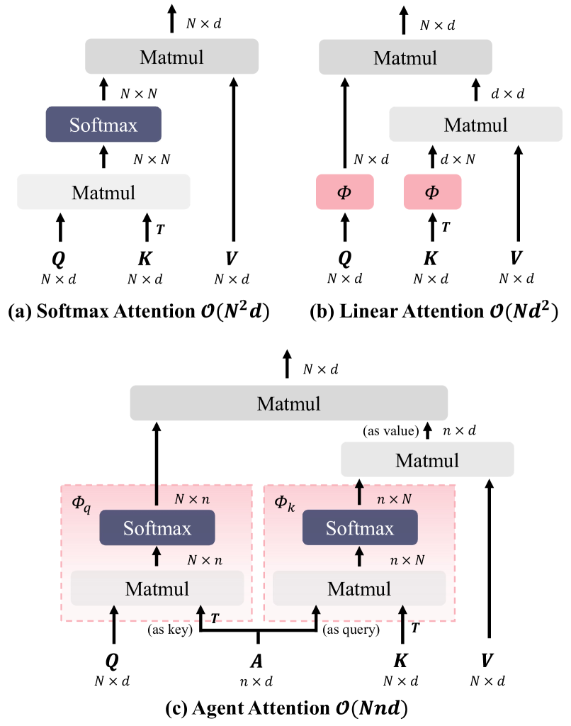
Figure 1: Difference between Softmax attention, Linear attention and Agent attention. Softmax attention computes the similarity between all query-key pairs, resulting in quadratic complexity. Linear attention applies mapping function $\phi(\cdot)$ to $Q$ and $K$ respectively to change the computation order, reducing complexity but suffering from insufficient expressive capability. Our Agent attention employs a small group of agent tokens to aggregate and broadcast global information, leading to an elegant integration of Softmax and linear attention and naturally enjoying the advantages of both high expressiveness and low computation complexity.

Originating from natural language processing, Transformer models have rapidly gained prominence in the field of computer vision in recent years, achieving significant success in image classification [13, 37, 15], object detection [39, 5], semantic segmentation [6, 43], and multimodal tasks [29].

Nevertheless, incorporating Transformers and self-attention into the visual domain presents formidable challenges. Modern Transformer models commonly employ Softmax attention [38], which computes the similarity between each query-key pair, resulting in quadratic computation complexity with respect to the number of tokens. As a result, directly applying Softmax attention with global receptive fields to the visual tasks can lead to unmanageable computational demands. To tackle this issue, existing works [39, 25, 41, 16, 50] attempt to reduce computation complexity by designing efficient attention patterns. As two representatives, Swin Transformer [25] reduces the receptive field and confines self-attention calculations to local windows. PVT [39] employs a sparse attention pattern to alleviate the computational burden by reducing the number of keys and values. Despite their effectiveness, these methods inevitably compromise the capability to model long-range relationships, and are still inferior to global self-attention.

In this paper, we innovatively introduce an additional set of tokens $A$ to the attention triplet $(Q,K,V)$, yielding a quadruplet attention paradigm $(Q,A,K,V)$, dubbed Agent Attention. As illustrated in Fig. 1(c), the resulting agent attention module is composed of two conventional Softmax attention operations. The first Softmax attention is applied to the triplet $(A,K,V)$, where the agent tokens $A$ serve as the queries to aggregate information from the value tokens $V$, with attention matrix calculated between $A$ and $K$. The second Softmax attention is performed on the triplet $(Q,A,V_{A})$, where $V_{A}$ is the result of the previous step, forming the final output of the proposed agent attention. Intuitively, the newly introduced tokens $A$ can be viewed as “agents” for the query tokens $Q$, as they directly collect information from $K$ and $V$, and then deliver the result to $Q$. The query tokens $Q$ no longer need to directly communicate with the original keys $K$ and values $V$. Hence we call the tokens $A$ the agent tokens.

Due to the intrinsic redundancy in global self-attention, the number of agent tokens can be designed to be much smaller than the number of query tokens. For example, we find that simply pooling the original query tokens to form the agent tokens works surprisingly well. This property endows agent attention with high efficiency, reducing the quadratic complexity (in the number of tokens) of Softmax attention to linear complexity. Meanwhile, the global context modelling capability is preserved. Interestingly, as illustrated in Fig. 1, the proposed agent attention can be viewed as a generalized from of linear attention, which explains how agent attention addresses the dilemma between efficiency and expressiveness from a novel perspective. In other words, agent attention seamlessly integrates Softmax and linear attention, and enjoys benefits from both worlds.

We empirically verify the effectiveness of our model across diverse vision tasks, including image classification, object detection, semantic segmentation and image generation. Our method yields substantial improvements in various tasks, particularly in high-resolution scenarios. Noteworthy, our agent attention can be directly plugged into pre-trained large diffusion models, and without any additional training, it not only accelerates the generation process, but also notably improves the generation quality.

2 Related Works

2.1 Vision Transformer

Since the inception of Vision Transformer [13], self-attention has made notable strides in the realm of computer vision. However, the quadratic complexity of the prevalent Softmax attention [38] poses a challenge in applying self-attention to visual tasks. Previous works proposed various remedies for this computational challenge. PVT [39] introduces sparse global attention, curbing computation cost by reducing the resolution of $K$ and $V$. Swin Transformer [25] restricts self-attention computations to local windows and employs shifted windows to model the entire image. NAT [16] emulates convolutional operations and calculates attention within the neighborhood of each feature. DAT [41] designs a deformable attention module to achieve a data-dependent attention pattern. BiFormer [50] uses bi-level routing attention to dynamically determine areas of interest for each query. GRL [21] employs a mixture of anchored stripe attention, window attention, and channel attention to achieve efficient image restoration.

However, These approaches inherently limit the global receptive field of self-attention or are vulnerable to specifically designed attention patterns, hindering their plug-and-play adaptability for general purposes.

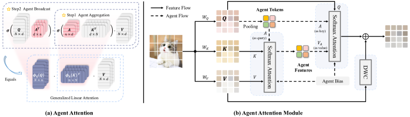
Figure 2: An illustration of our agent attention and agent attention module. (a) Agent attention uses agent tokens to aggregate global information and distribute it to individual image tokens, resulting in a practical integration of Softmax and linear attention. $\rm{\sigma}(\cdot)$ represents Softmax function. In (b), we depict the information flow of agent attention module. As a showcase, we acquire agent tokens through pooling. Subsequently, agent tokens are utilized to aggregate information from $V$, and $Q$ queries features from the agent features. In addition, agent bias and DWC are adopted to add positional information and maintain feature diversity.

2.2 Linear Attention

In contrast to the idea of restricting receptive fields, linear attention directly addresses the computational challenge by reducing computation complexity. The pioneer work [19] discards the Softmax function and replaces it with a mapping function $\phi$ applied to $Q$ and $K$, thereby reducing the computation complexity to $\mathcal{O}(N)$. However, such approximations led to substantial performance degradation. To tackle this issue, Efficient Attention [34] applies the Softmax function to both $Q$ and $K$. SOFT [27] and Nyströmformer [44] employ matrix decomposition to further approximate Softmax operation. Castling-ViT [45] uses Softmax attention as an auxiliary training tool and fully employs linear attention during inference. FLatten Transformer [14] proposes focused function and adopts depthwise convolution to preserve feature diversity.

While these methods are effective, they continue to struggle with the issue of limited expressive power of linear attention. In the paper, rather than enhancing Softmax or linear attention, we propose a novel attention paradigm which integrates these two attention types, achieving superior performance in various tasks.

3 Preliminaries

In this section, we first review the general form of self-attention in modern vision Transformers and briefly analyze the pros and cons of Softmax and linear attention.

3.1 General Form of Self-Attention

With an input of $N$ tokens represented as $x\in\mathbb{R}^{N\times C}$, self-attention can be formulated as follows in each head:

$$\begin{split}Q=xW_{Q},K=xW_{K},V=xW_{V},\\ O_{i}=\sum_{j=1}^{N}\ \frac{{\rm Sim}{\left(Q_{i},K_{j}\right)}}{\sum_{j=1}^{N}\ {\rm Sim}{\left(Q_{i},K_{j}\right)}}V_{j},\end{split}$$ (1)

where $W_{Q/K/V}\!\in\!\mathbb{R}^{C\times d}$ denote projection matrices, $C$ and $d$ are the channel dimension of module and each head, and ${\rm Sim}{\left(\cdot,\cdot\right)}$ represents the similarity function.

3.2 Softmax Attention and Linear Attention

When using ${\rm Sim}\left(Q,K\right)\!=\!{\rm exp}({QK^{T}}/{\sqrt{d}})$ in Eq. 1, it becomes Softmax attention [38], which has been highly successful in modern vision Transformer designs. However, Softmax attention compels to compute the similarity between all query-key pairs, resulting in $\mathcal{O}(N^{2})$ complexity. Consequently, using Softmax attention with a global receptive field leads to overwhelming computation complexity. To tackle this issue, previous works attempted to reduce the number of tokens $N$ by designing sparse global attention [39, 40] or window attention [25, 12] patterns. While effective, these strategies unavoidably compromise the self-attention’s capability for long-range modeling.

Comparably, linear attention [19] efficiently addresses the computation challenge with a linear complexity of $\mathcal{O}(N)$. Specifically, carefully designed mapping functions are applied to $Q$ and $K$ respectively, i.e., ${\rm Sim}\left(Q,K\right)=\phi(Q)\phi(K)^{T}$. This gives us the opportunity to change the computation order from $(\phi(Q)\phi(K)^{T})V$ to $\phi(Q)(\phi(K)^{T}V)$ based on the associative property of matrix multiplication. As illustrated in Fig. 1, by doing so, the computation complexity with respect to token number is reduced to $\mathcal{O}(N)$.

However, designing effective mapping function $\phi(\cdot)$ proves to be a nontrivial task. Simple functions [34] such as ReLU lead to significant performance drop, whereas more intricate designs [7] or matrix decomposition methods [27, 44] may introduce extra computation overhead. In general, current linear attention approaches are still inferior to Softmax attention, limiting their practical application.

4 Agent Transformer

As discussed in Sec. 3, Softmax and linear attention suffer from either excessive computation complexity or insufficient model expressiveness. Previous research commonly treated these two attention paradigms as distinct approaches and attempted to either reduce the computation cost of Softmax attention or enhance the performance of linear attention. In this section, we propose a new attention paradigm named Agent Attention, which practically forms an elegant integration of Softmax and linear attention, enjoying benefits from both linear complexity and high expressiveness.

4.1 Agent Attention

To simplify, we abbreviate Softmax and linear attention as:

$$\begin{split}O^{\rm S}\!=&\ {\rm\sigma}(QK^{T})V\triangleq{\rm Attn}^{\rm S}(Q,K,V),\\ O^{\rm\phi}\!=&\ \phi(Q)\phi(K)^{T}V\triangleq{\rm Attn}^{\rm\phi}(Q,K,V),\\ \end{split}$$ (2)

where $Q,K,V\in\mathbb{R}^{N\times C}$ denote query, key and value matrices and $\rm{\sigma}(\cdot)$ represents Softmax function. Then our agent attention can be written as:

$$\begin{split}O^{\rm A}=&\ \underbrace{{\rm Attn}^{\rm S}(Q,A,\underbrace{{\rm Attn}^{\rm S}(A,K,V)}_{\rm Agent\ Aggregation})}_{\rm Agent\ Broadcast}.\\ \end{split}$$ (3)

It is equivalent to:

$$\begin{split}O^{\rm A}=&\ {\rm\sigma}(QA^{T})\ {\rm\sigma}(AK^{T})\ V\\ =&\ {\phi}_{q}(Q){\phi}_{k}(K)^{T}V\\ =&\ \underbrace{{\rm Attn}^{\rm\phi_{q/k}}(Q,K,V)}_{\rm Generalized\ Linear\ Attn},\\ \end{split}$$ (4)

where $A\in\mathbb{R}^{n\times C}$ is our newly defined agent tokens.

As shown in Eq. 3 and Fig. 2(a), our agent attention consists of two Softmax attention operations, namely agent aggregation and agent broadcast. Specifically, we initially treat agent tokens $A$ as queries and perform attention calculations between $A$, $K$, and $V$ to aggregate agent features $V_{A}$ from all values. Subsequently, we utilize $A$ as keys and $V_{A}$ as values in the second attention calculation with the query matrix $Q$, broadcasting the global information from agent features to every query token and obtaining the final output $O$. In this way, we avoid the computation of pairwise similarities between $Q$ and $K$ while preserving information exchange between each query-key pair through agent tokens.

The newly defined agent tokens $A$ essentially serve as the agent for $Q$, aggregating global information from $K$ and $V$, and subsequently broadcasting it back to $Q$. Practically, we set the number of agent tokens $n$ as a small hyper-parameter, achieving a linear computation complexity of $\mathcal{O}(Nnd)$ relative to the number of input features $N$ while maintaining global context modeling capability.

Interestingly, as shown in Eq. 4 and Fig. 2(a), we practically integrate the powerful Softmax attention and efficient linear attention, establishing a generalized linear attention paradigm by employing two Softmax attention operations, with the equivalent mapping function defined as ${\phi}_{q}(Q)={\rm\sigma}(QA^{T}),{\phi}_{k}(K)={\left({\rm\sigma}(AK^{T})\right)}^{T}$.

In practice, agent tokens can be acquired through different methods, such as simply setting as a set of learnable parameters or extracting from input features through pooling. It is worth noticing that more advanced techniques like deformed points [41] or token merging [3] can also be used to obtain agent tokens. In this paper, we employ the simple pooling strategy to obtain agent tokens, which already works surprisingly well.

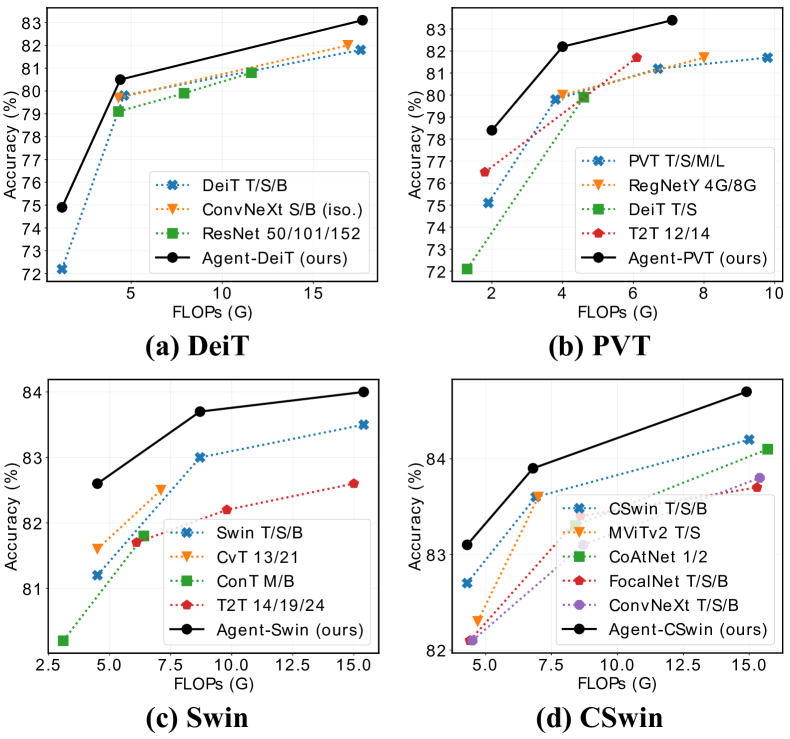
Method	Reso	#Params	FLOPs	Top-1
DeiT-T [37]	${224}^{2}$	5.7M	1.2G	72.2
Agent-DeiT-T	${224}^{2}$	6.0M	1.2G	74.9 (+2.7)
DeiT-S	${224}^{2}$	22.1M	4.6G	79.8
Agent-DeiT-S	${224}^{2}$	22.7M	4.4G	80.5 (+0.7)
PVT-T [39]	${224}^{2}$	13.2M	1.9G	75.1
Agent-PVT-T	${224}^{2}$	11.6M	2.0G	78.4 (+3.3)
PVT-S	${224}^{2}$	24.5M	3.8G	79.8
Agent-PVT-S	${224}^{2}$	20.6M	4.0G	82.2 (+2.4)
PVT-M	${224}^{2}$	44.2M	6.7G	81.2
Agent-PVT-M	${224}^{2}$	35.9M	7.0G	83.4 (+2.2)
PVT-L	${224}^{2}$	61.4M	9.8G	81.7
Agent-PVT-L	${224}^{2}$	48.7M	10.4G	83.7 (+2.0)
Swin-T [25]	${224}^{2}$	29M	4.5G	81.3
Agent-Swin-T	${224}^{2}$	29M	4.5G	82.6 (+1.3)
Swin-S	${224}^{2}$	50M	8.7G	83.0
Agent-Swin-S	${224}^{2}$	50M	8.7G	83.7 (+0.7)
Swin-B	${224}^{2}$	88M	15.4G	83.5
Agent-Swin-B	${224}^{2}$	88M	15.4G	84.0 (+0.5)
Swin-B	${384}^{2}$	88M	47.0G	84.5
Agent-Swin-B	${384}^{2}$	88M	46.3G	84.9 (+0.4)
CSwin-B [12]	${224}^{2}$	78M	15.0G	84.2
Agent-CSwin-B	${224}^{2}$	73M	14.9G	84.7 (+0.5)
CSwin-B	${384}^{2}$	78M	47.0G	85.4
Agent-CSwin-B	${384}^{2}$	73M	46.3G	85.8 (+0.4)

Figure 3: Comparison of different models on ImageNet-1K. See the full comparison table in Appendix.

4.2 Agent Attention Module

Agent attention inherits the merits of both Softmax and linear attention. In practical use, we further make two improvements to maximize the potential of agent attention.

Agent Bias. In order to better utilize positional information, we present a carefully designed Agent Bias for our agent attention. Specifically, inspired by RPE [33], we introduce agent bias within the attention calculation, i.e.,

$$\begin{split}O^{\rm A}\!=\ &{\rm\sigma}(QA^{T}\!\!+\!B_{2})\ {\rm\sigma}(AK^{T}\!\!+\!B_{1})\ V,\\ \end{split}$$ (5)

where $B_{1}\in\mathbb{R}^{n\times N},B_{2}\in\mathbb{R}^{N\times n}$ are our agent biases. For parameter efficiency, we construct each agent bias using three bias components rather than directly setting $B_{1},B_{2}$ as learnable parameters (see Appendix). Agent bias augments the vanilla agent attention with spatial information, helping different agent tokens to focus on diverse regions. As shown in Tab. 6, significant improvements can be observed upon the introduction of our agent bias terms.

Diversity Restoration Module. Although agent attention benefits from both low computation complexity and high model expressiveness, as generalized linear attention, it also suffers from insufficient feature diversity [14]. As a remedy, we follow [14] and adopt a depthwise convolution (DWC) module to preserve feature diversity.

Agent Attention Module. Building upon these designs, we propose a novel attention module named Agent Attention Module. As illustrated in Fig. 2(b), our module is composed of three parts, namely pure agent attention, agent bias and the DWC module. Our module can be formulated as:

$$\begin{split}O=&\ {\rm\sigma}(QA^{T}\!\!+\!B_{2})\ {\rm\sigma}(AK^{T}\!\!+\!B_{1})\ V+{\rm DWC}(V),\end{split}$$ (6)

where $Q,K,V\in\mathbb{R}^{N\times C}$,$\ B_{1}\!\in\!\mathbb{R}^{n\times N}$,$\ B_{2}\!\in\!\mathbb{R}^{N\times n}$ and $A=\ {\rm Pooling(Q)}\in\mathbb{R}^{n\times C}$.

Combining the merits of Softmax and linear attention, our module offers the following advantages:

(1) Efficient computation and high expressive capability. Previous work usually viewed Softmax attention and linear attention as two different attention paradigms, aiming to address their respective limitations. As a seamless integration of these two attention forms, our agent attention naturally inherits the merits of the two, enjoying both low computation complexity and high model expression ability at the same time.

(2) Large receptive field. Our module can adopt a large receptive field while maintaining the same amount of computation. Modern vision Transformer models typically resort to sparse attention [39, 40] or window attention [25, 12] to mitigate the computation burden of Softmax attention. Benefited from linear complexity, our model can enjoy the advantages of a large, even global receptive field while maintaining the same computation.

4.3 Implementation

Our agent attention module can serve as a plug-in module and can be easily adopted on a variety of modern vision Transformer architectures. As a showcase, we empirically apply our method to four advanced and representative Transformer models including DeiT [37], PVT [39], Swin [25] and CSwin [12]. We also apply agent attention to Stable Diffusion [30] to accelerate image generation. Detailed model architectures are shown in Appendix.

5 Experiments

To verify the effectiveness of our method, we conduct experiments on ImageNet-1K classification [9], ADE20K semantic segmentation [49], and COCO object detection [22]. Additionally, we integrate agent attention into the state-of-the-art generation model, Stable Diffusion [30]. Furthermore, we construct high-resolution models with large receptive fields to maximize the benefits of agent attention. In addition, sufficient ablation experiments are conducted to show the effectiveness of each design.

5.1 ImageNet-1K Classification

ImageNet [9] comprises 1000 classes, with 1.2 million training images and 50,000 validation images. We implement our module on four representative vision Transformers and compare the top-1 accuracy on the validation split with various state-of-the-art models.

Training settings are shown in Appendix.

Results. As depicted in Fig. 3, substituting Softmax attention with agent attention in various models results in significant performance improvements. For instance, Agent-PVT-S surpasses PVT-L while using just 30% of the parameters and 40% of the FLOPs. Agent-Swin-T/S outperform Swin-T/S by 1.3% and 0.7% while maintaining similar FLOPs. These results unequivocally prove that our approach has robust advantages and is adaptable to diverse architectures.

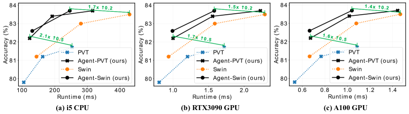
Figure 4: Accuracy-Runtime curve on ImageNet. Runtime is tested with image resolution 224×224.

(a) Mask R-CNN Object Detection on COCO
Method	FLOPs	Sch.	APb	AP${}^{b}_{\text{50}}$	AP${}^{b}_{\text{75}}$	APm	AP${}^{m}_{\text{50}}$	AP${}^{m}_{\text{75}}$
PVT-T	240G	1x	36.7	59.2	39.3	35.1	56.7	37.3
Agent-PVT-T	230G	1x	41.4	64.1	45.2	38.7	61.3	41.6
PVT-S	305G	1x	40.4	62.9	43.8	37.8	60.1	40.3
Agent-PVT-S	293G	1x	44.5	67.0	49.1	41.2	64.4	44.5
PVT-M	392G	1x	42.0	64.4	45.6	39.0	61.6	42.1
Agent-PVT-M	400G	1x	45.9	67.8	50.4	42.0	65.0	45.4
PVT-L	494G	1x	42.9	65.0	46.6	39.5	61.9	42.5
Agent-PVT-L	510G	1x	46.9	69.2	51.4	42.8	66.2	46.2
Swin-T	267G	1x	43.7	66.6	47.7	39.8	63.3	42.7
Agent-Swin-T	276G	1x	44.6	67.5	48.7	40.7	64.4	43.4
Swin-T	267G	3x	46.0	68.1	50.3	41.6	65.1	44.9
Agent-Swin-T	276G	3x	47.3	69.5	51.9	42.7	66.4	46.2
Swin-S	358G	1x	45.7	67.9	50.4	41.1	64.9	44.2
Agent-Swin-S	364G	1x	47.2	69.6	52.3	42.7	66.6	45.8
(b) Cascade Mask R-CNN Object Detection on COCO
Method	FLOPs	Sch.	APb	AP${}^{b}_{\text{50}}$	AP${}^{b}_{\text{75}}$	APm	AP${}^{m}_{\text{50}}$	AP${}^{m}_{\text{75}}$
Swin-T	745G	1x	48.1	67.1	52.2	41.7	64.4	45.0
Agent-Swin-T	755G	1x	49.2	68.6	53.2	42.7	65.6	45.9
Swin-T	745G	3x	50.4	69.2	54.7	43.7	66.6	47.3
Agent-Swin-T	755G	3x	51.4	70.2	55.9	44.5	67.6	48.4
Swin-S	837G	3x	51.9	70.7	56.3	45.0	68.2	48.8
Agent-Swin-S	843G	3x	52.6	71.3	57.1	45.5	68.9	49.2
Swin-B	981G	3x	51.9	70.5	56.4	45.0	68.1	48.9
Agent-Swin-B	990G	3x	52.6	71.1	57.1	45.3	68.6	49.2

Table 1: Results on COCO dataset. The FLOPs are computed over backbone, FPN and detection head with an input resolution of 1280$\times$800. We appropriately increase the number of agent tokens in downstream tasks to better model high-resolution images.

Inference Time. We further conduct real speed measurements by deploying the models on various devices. As Fig. 4 illustrates, our models attain inference speeds 1.7 to 2.1 times faster on the CPU while simultaneously improving performance. On RTX3090 GPU and A100 GPU, our models also achieve 1.4x to 1.7x faster inference speeds.

5.2 Object Detection

COCO [22] object detection and instance segmentation dataset has 118K training and 5K validation images. We apply our model to RetinaNet [23], Mask R-CNN [17] and Cascade Mask R-CNN [4] frameworks to evaluate the performance of our method. A series of experiments are conducted utilizing both 1x and 3x schedules with different detection heads. As depicted in Tab. 1, our model exhibits consistent enhancements across all configurations. Agent-PVT outperforms PVT models with an increase in box AP ranging from +3.9 to +4.7, while Agent-Swin surpasses Swin models by up to +1.5 box AP. These substantial improvements can be attributed to the large receptive field brought by our design, demonstrating the effectiveness of agent attention in high-resolution scenarios.

5.3 Semantic Segmentation

Semantic Segmentation on ADE20K
Backbone	Method	FLOPs	#Params	mIoU	mAcc
PVT-T	S-FPN	158G	17M	36.57	46.72
Agent-PVT-T	S-FPN	147G	15M	40.18	51.76
PVT-S	S-FPN	225G	28M	41.95	53.02
Agent-PVT-S	S-FPN	211G	24M	44.18	56.17
PVT-L	S-FPN	420G	65M	43.49	54.62
Agent-PVT-L	S-FPN	434G	52M	46.52	58.50
Swin-T	UperNet	945G	60M	44.51	55.61
Agent-Swin-T	UperNet	954G	61M	46.68	58.53

Table 2: Results of semantic segmentation. The FLOPs are computed over encoders and decoders with an input image at the resolution of 512$\times$2048. S-FPN is short for SemanticFPN [20] model.

ADE20K [49] is a well-established benchmark for semantic segmentation which encompasses 20K training images and 2K validation images. We apply our model to two exemplary segmentation models, namely SemanticFPN [20] and UperNet [42]. The results are presented in Tab. 2. Remarkably, our Agent-PVT-T and Agent-Swin-T achieve +3.61 and +2.17 higher mIoU than their counterparts. The results show that our model is compatible with various segmentation backbones and consistently achieves improvements.

5.4 Agent Attention for Stable Diffusion

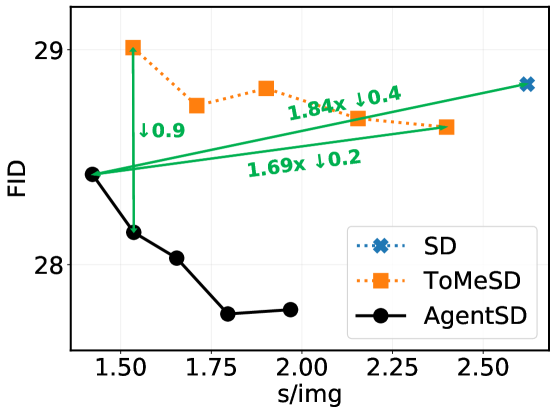
Figure 5: Quantitative Results of Stable Diffusion, ToMeSD and our AgentSD. For ToMeSD, we take the merging ratios $\{0.1,0.2,0.3,0.4,0.5\}$ to construct five different models. Furthermore, we apply agent attention to each ToMeSD model to obtain the corresponding AgentSD model.

The advent of diffusion models makes it possible to generate high-resolution and high-quality images. However, current diffusion models mainly use the original Softmax attention with a global receptive field, resulting in huge computation cost and slow generation speed. In the light of this, we apply our agent attention to Stable Diffusion [30], hoping to improve the generation speed of the model. Surprisingly, after simple adjustments, the Stable Diffusion model using agent attention, dubbed AgentSD, shows a significant improvement in generation speed and produces even better image quality without any extra training.

Applying agent attention to Stable Diffusion. We practically apply agent attention to ToMeSD model [1]. ToMeSD reduces the number of tokens before attention calculation in Stable Diffusion, enhancing generation speed. Nonetheless, the post-merge token count remains considerable, resulting in continued complexity and latency. Hence, we replace the Softmax attention employed in ToMeSD model with our agent attention to further enhance speed. We experimentally find that when producing agent tokens through token merging [3], our agent attention can be directly applied to Stable Diffusion and ToMeSD model without any extra training. However, we are unable to apply the agent bias and DWC in this way. As a remedy, we make two simple adjustments to the agent attention, which are described in detail in Appendix. In addition, we get a significant boost by applying agent attention during early diffusion generation steps and keeping the later steps unchanged.

Quantitative Results. We follow [1] and quantitatively compare AgentSD with Stable Diffusion and ToMeSD. As displayed in Fig. 5, ToMeSD accelerates Stable Diffusion while maintaining similar image quality. AgentSD not only further accelerates ToMeSD but also significantly enhances image generation quality. Specifically, while maintaining superior image generation quality, AgentSD achieves 1.84x and 1.69x faster generation speeds compared to Stable Diffusion and ToMeSD, respectively. At an equivalent generation speed, AgentSD produces samples with a 0.9 lower FID score compared to ToMeSD. See the experimental details and full comparison table in Appendix.

Figure 6: Samples generated by Stable Diffusion, ToMeSD ($r=40\%$) and AgentSD ($r=40\%$). The prompt is “A high quality photograph of a {cls}.”.

Visualization. We present some visualizations in Fig. 6. AgentSD noticeably reduces ambiguity and generation errors in comparison to Stable Diffusion and ToMeSD. For instance, in the first column, Stable Diffusion and ToMeSD produce birds with one leg and two tails, while AgentSD’s sample does not exhibit this issue. In the third column, when provided with the prompt “A high quality photo of a mitten.”, Stable Diffusion and ToMeSD erroneously generate a cat, whereas AgentSD produces the correct image.

AgentSD for finetuning. We apply agent attention to SD-based Dreambooth [31] to verify its performance under finetuning. When finetuned, agent attention can be integrated into all diffusion generation steps, reaching 2.2x acceleration in generation speed compared to the original Dreambooth. Refer to Appendix for details.

5.5 Large Receptive Field and High Resolution

Large Receptive Field. Modern vision Transformers often confine self-attention calculation to local windows to reduce computation complexity, such as Swin [25]. In Tab. 3, we gradually enlarge the window size of Agent-Swin-T, ranging from $7^{2}$ to $56^{2}$. Clearly, as the receptive field expands, the model’s performance consistently improves. This indicates that while the window attention pattern is effective, it inevitably compromises the long-range modeling capability of self-attention and remains inferior to global attention. Due to the linear complexity of agent attention, we can benefit from a global receptive field while preserving identical computation complexity.

	Window	FLOPs	#Param	Acc.	Diff.
Agent-Swin-T	$7^{2}$	4.5G	29M	82.0	-0.6
	${14}^{2}$	4.5G	29M	82.2	-0.4
	${28}^{2}$	4.5G	29M	82.4	-0.2
	${56}^{2}$	4.5G	29M	82.6	Ours
Swin-T	$7^{2}$	4.5G	29M	81.3	-1.3

Table 3: Ablation on window size based on Agent-Swin-T.

Method	Reso	#Params	Flops	Top-1
DeiT-B [37]	${224}^{2}$	86.6M	17.6G	81.8
DeiT-S	${416}^{2}$	22.2M	18.8G	82.9 (+1.1)
Agent-DeiT-B	${224}^{2}$	87.2M	17.6G	82.0 (+0.2)
Agent-DeiT-S	${448}^{2}$	23.1M	17.7G	83.1 (+1.3)
PVT-L [39]	${224}^{2}$	61.4M	9.8G	81.7
PVT-M	${256}^{2}$	44.3M	8.8G	82.2 (+0.5)
Agent-PVT-L	${224}^{2}$	48.7M	10.4G	83.7 (+2.0)
Agent-PVT-M	${256}^{2}$	36.1M	9.2G	83.8 (+2.1)
Swin-B [25]	${224}^{2}$	88M	15.4G	83.5
Swin-S	${288}^{2}$	50M	14.7G	83.7 (+0.2)
Agent-Swin-B	${224}^{2}$	88M	15.4G	84.0 (+0.5)
Agent-Swin-S	${288}^{2}$	50M	14.6G	84.1 (+0.6)

Table 4: Scaling up by increasing resolution. All these models are trained for 300 epochs from scratch.

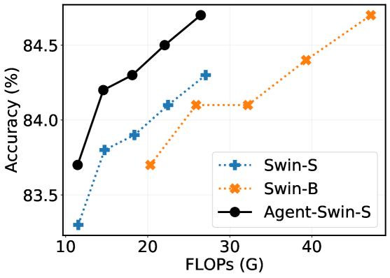
Figure 7: Increasing resolution to $\{256^{2},288^{2},320^{2},352^{2},$ $384^{2}\}$. All these models are finetuned for 30 epochs from the corresponding $224^{2}$ resolution models.

High Resolution. Limited by the quadratic complexity of Softmax attention, current vision Transformer models usually scale up by increasing model depth and width. Building on insights from [36], we discover that enhancing resolution might be a more effective approach for scaling vision Transformers, particularly those employing agent attention with global receptive fields. As shown in Tab. 4, Agent-DeiT-B achieves a 0.2 accuracy gain compared to DeiT-B, whereas Agent-DeiT-S at $448^{2}$ resolution attains an accuracy of 83.1 with only a quarter of the parameters. We observed analogous trends when scaling the resolution of Agent-PVT-M and Agent-Swin-S. In Fig. 7, we progressively increase the resolution of Agent-Swin-S, Swin-S, and Swin-B. It is evident that in high-resolution scenarios, our model consistently delivers notably superior outcomes.

5.6 Comparison with Other Linear Attention

(a) Comparison on DeiT-T Setting
Linear Attention	FLOPs	#Param	Acc.
Hydra Attn [2]	1.1G	5.7M	68.3
Efficient Attn [34]	1.1G	5.7M	70.2
Linear Angular Attn [45]	1.1G	5.7M	70.8
Focused Linear Attn [14]	1.1G	6.1M	74.1
Ours	1.2G	6.0M	74.9
(b) Comparison on Swin-T Setting
Linear Attention	FLOPs	#Param	Acc.
Hydra Attn [2]	4.5G	29M	80.7
Efficient Attn [34]	4.5G	29M	81.0
Linear Angular Attn [45]	4.5G	29M	79.4
Focused Linear Attn [14]	4.5G	29M	82.1
Ours	4.5G	29M	82.6

Table 5: Comparison of different linear attention designs on DeiT-Tiny and Swin-Tiny structures.

We conduct a comparison of our agent attention with other linear attention methods using DeiT-T and Swin-T. As depicted in Tab. 5, substituting the Softmax attention employed by DeiT-T and Swin-T with various linear attention methods usually results in notable performance degradation. Remarkably, our models outperform all other methods as well as the Softmax baseline.

5.7 Ablation Study

In this section, we ablate the key components in our agent attention module to verify the effectiveness of these designs. We report the results on ImageNet-1K classification based on Agent-Swin-T.

	FLOPs	#Param	Acc.	Diff.
Vanilla Linear Attention	4.5G	29M	77.8	-4.8
Agent Attention	4.5G	29M	79.0	-3.6
$+$  Agent Bias	4.5G	29M	81.1	-1.5
$+$  DWC	4.5G	29M	82.6	Ours
Swin-T	4.5G	29M	81.3	-1.3

Table 6: Ablation on each module of agent attention.

Agent attention, agent bias and DWC. We first assess the effectiveness of our agent attention’s three key designs. We substitute Softmax attention in Swin-T with vanilla linear attention, followed by a gradual introduction of agent attention, agent bias, and DWC to create Agent-Swin-T. As depicted in Tab. 6, the inclusion of these three designs led to respective accuracy gains of 1.2, 2.1, and 1.5.

	FLOPs	#Param	Acc.	Diff.
Static Agent	4.5G	29M	82.2	-0.4
Dynamic Agent	4.5G	29M	82.6	Ours
Swin-T	4.5G	29M	81.3	-1.3

Table 7: Ablation on the type of agent tokens.

The type of agent tokens. As discussed in Sec. 4.1, agent tokens can be acquired through various methods. As a showcase, we roughly categorize agent tokens into two types: static and dynamic. The former sets agent tokens as learnable parameters, while the latter uses pooling to acquire agent tokens. As illustrated in Tab. 7, dynamic agent tokens yield better results.

Num of Agent Tokens				FLOPS	#Param	Acc.	Diff.
Stage1	Stage2	Stage3	Stage4
49	49	49	49	4.7G	29M	82.6	-0.0
9	16	49	49	4.5G	29M	82.6	Ours
9	16	25	49	4.5G	29M	82.2	-0.4
4	9	49	49	4.5G	29M	82.4	-0.2
Swin-T				4.5G	29M	81.3	-1.3

Table 8: Ablation on the number of agent tokens.

Ablation on number of agent tokens. The model’s computation complexity can be modulated by varying the number of agent tokens. As shown in Tab. 8, we observe that judiciously reducing the number of agent tokens in the model’s shallower layers has no adverse effect on performance. However, reducing agent tokens in deeper layers results in performance degradation.

Stages w/ Agent Attn				FLOPS	#Param	Acc.	Diff.
Stage1	Stage2	Stage3	Stage4
$\checkmark$				4.5G	29M	81.7	-0.9
$\checkmark$	$\checkmark$			4.5G	29M	81.8	-0.8
$\checkmark$	$\checkmark$	$\checkmark$		4.5G	29M	82.6	Ours
$\checkmark$	$\checkmark$	$\checkmark$	$\checkmark$	4.5G	29M	82.5	-0.1
Swin-T				4.5G	29M	81.3	-1.3

Table 9: Ablation on applying agent attention module on different stages of the Swin-T structure.

Agent attention at different stages. We substitute Softmax attention with our agent attention at different stages. As depicted in Tab. 9, substituting the first three stages results in a performance gain of 1.3, while replacing the final stage marginally decreases overall accuracy. We attribute this outcome to the larger resolutions in the first three stages, which are more conducive to agent attention module with a global receptive field.

6 Conclusion

This paper presents a new attention paradigm dubbed Agent Attention, which is applicable across a variety of vision Transformer models. As an elegant integration of Softmax and linear attention, agent attention enjoys both high expressive power and low computation complexity. Extensive experiments on image classification, semantic segmentation, and object detection unequivocally confirm the effectiveness of our approach, particularly in high-resolution scenarios. When integrated with Stable Diffusion, our agent attention accelerates image generation and substantially enhances image quality without any extra training. Due to its linear complexity with respect to the number of tokens and its strong representation power, agent attention may pave the way for challenging tasks with super long token sequences, such as video modelling and multi-modal foundation models.

Appendix

A. Composition of Agent Bias

As mentioned in the main paper, to better utilize positional information, we present a carefully designed Agent Bias for our agent attention, i.e.,

$$\begin{split}O^{\rm A}\!=\ &{\rm\sigma}(QA^{T}\!\!+\!B_{2})\ {\rm\sigma}(AK^{T}\!\!+\!B_{1})\ V,\\ \end{split}$$ (7)

where $B_{1}\in\mathbb{R}^{n\times N},B_{2}\in\mathbb{R}^{N\times n}$ are our agent biases. For parameter efficiency, we construct each agent bias using three bias components rather than directly setting $B_{1},B_{2}$ as learnable parameters. For instance, values in $B_{1}$ are derived from column bias $B_{1c}\in\mathbb{R}^{n\times 1\times w}$, row bias $B_{1r}\in\mathbb{R}^{n\times h\times 1}$ and block bias $B_{1b}\in\mathbb{R}^{n\times h_{0}\times w_{0}}$, where $h,w$ are the height and width of feature map or attention window, while $h_{0},w_{0}$ are predefined hyperparameters much smaller than $h,w$. During the computation of attention weights, $B_{1c},B_{1r},B_{1b}$ are resized to $B^{\prime}_{1c},B^{\prime}_{1r},B^{\prime}_{1b}\in\mathbb{R}^{n\times h\times w}$ by repeating or interpolating, and $B_{1}=(B^{\prime}_{1c}+B^{\prime}_{1r}+B^{\prime}_{1b}).{\rm reshape}(n,N)$ is used as the full agent bias.

B. Agent Attention for Stable Diffusion

B.1. Adjustments

As discussed in the main paper, when producing agent tokens through token merging, our agent attention can be directly applied to the Stable Diffusion model without any extra training. However, we are unable to apply the agent bias and DWC without training. As a remedy, we make two simple adjustments to the agent attention. On the one hand, we change our agent attention module from

$$\begin{split}O=&\ {\rm\sigma}(QA^{T}\!\!+\!B_{2})\ {\rm\sigma}(AK^{T}\!\!+\!B_{1})\ V+{\rm DWC}(V),\end{split}$$ (8)

to

$$\begin{split}O=&\ {\rm\sigma}(QA^{T})\ {\rm\sigma}(AK^{T})\ V+kV,\end{split}$$ (9)

where $k$ is a predefined hyperparameter. On the other hand, compared to the original softmax attention, the two softmax attention operations of agent attention may result in smoother feature distribution without training. In the light of this, we slightly increase the scale used for the second Softmax attention, i.e., agent broadcast.

B.2. Experiment Details

To quantitatively compare AgentSD with Stable Diffusion and ToMeSD, we follow [1] and employ Stable Diffusion v1.5 to generate 2,000 $512^{2}$ images of ImageNet-1k [9] classes, featuring two images per class, using 50 PLMS [24] diffusion steps with a cfg scale [11] of 7.5. Subsequently, we calculate FID [18] scores between these 2,000 samples and 50,000 ImageNet-1k validation examples, employing [32]. To assess speed, we calculate the average generation time of all 2,000 samples on a single RTX4090 GPU.

Complete quantitative results are presented in Tab. 10. Compared to SD and ToMeSD, our AgentSD not only accelerates generation and reduces memory usage, but also significantly improves image generation quality.

Method	r	FID	s/img	GB/img
SD [30]	0	28.84	2.62	3.13
ToMeSD [1]	0.1	28.64	2.40	2.55
	0.2	28.68	2.15	2.03
	0.3	28.82	1.90	2.09
	0.4	28.74	1.71	1.69
	0.5	29.01	1.53	1.47
	0.1	27.79	1.97	1.77
	0.2	27.77	1.80	1.60
AgentSD	0.3	28.03	1.65	2.05
	0.4	28.15	1.54	1.55
	0.5	28.42	1.42	1.21

Table 10: Quantitative Results of Stable Diffusion, ToMeSD and our AgentSD. GB/img is measured as the total memory usage change when increasing batch size by 1.

B.3. Ablation

We further ablate the adjustments we made when applying agent attention to Stable Diffusion. As evident in Tab. 11 and Tab. 12, both adjustments to agent attention enhance the quality of AgentSD generation. Tab. 13 demonstrates that applying agent attention in the early stages yields substantial performance enhancements.

$k$	0	0.025	0.075	0.15
FID	28.80	28.67	28.42	28.61

Table 11: Ablation on factor $k$ of Eq. 9.

Scale	$d^{-0.5}$	$d^{-0.25}$	$d^{-0.15}$	$d^{-0.05}$
FID	28.86	28.64	28.42	28.60

Table 12: Ablation on scale used for the second Softmax attention.

Steps	early 20%	early 40%	early 60%	early 80%
FID	28.58	28.42	28.83	29.77
s/img	1.50	1.42	1.39	1.34

Table 13: Ablation on how many diffusion steps to apply agent attention.

B.4. AgentSD for finetuning

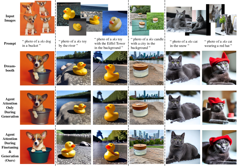
Figure 8: Samples generated by Dreambooth and our Agent Dreambooth with the same seed. In the second-to-last line, we apply agent attention to all diffusion steps only during generation, leading to a slight decline in image quality as expected. In the last row, agent attention is incorporated into all steps in both finetuning and generation, resulting in a 2.2x speedup without compromising image quality. Zoom in for best view.

Our agent attention module is also applicable in finetuning scenarios. To verify this, we select subject-driven task as an example and apply agent attention to SD-based Dreambooth [31]. We experimentally find that finetuning enables the integration of the agent attention module into all diffusion generation steps, reaching 2.2x acceleration in generation speed compared to the original Dreambooth without sacrificing image quality. Additionally, time and memory cost during finetuning can be reduced as well.

Task and baseline. The diffusion subject-driven generation task entails maintaining the appearance of a given subject while generating novel renditions of it in different contexts, e.g., generating a photo of your pet dog dancing. Dreambooth [31] effectively addresses this task by finetuning a pretrained text-to-image diffusion model, binding a unique identifier with the given subject. Novel images of the subject can then be synthesized with the unique identifier.

Applying agent attention to Dreambooth. As previously discussed, Dreambooth[31] involves an additional finetuning process. We explore two approaches to applying agent attention to Dreambooth: (1) applying it only during generation and (2) applying it during both finetuning and generation. The first method is the same as the AgentSD detailed in the main paper, where we commonly apply agent attention to the early 40% of generation steps, achieving around a 1.7x speedup (merging ratio $r=0.4$). However, applying agent attention to more diffusion steps for further acceleration leads to a decrease in image details and quality, as shown in Tab. 13 and the penultimate line of Fig. 8. Conversely, adopting the second approach, where the agent attention module is applied to all steps in both finetuning and generation, results in a 2.2x speedup in generation without sacrificing performance. Additionally, both time and memory costs in finetuning are reduced by around 15%, enabling model finetuning with less than 12GB of GPU memory in approximately 7 minutes on a single RTX4090 GPU. The last row in Fig. 8 shows the results of this setting.

Dataset and experiment details. We adopt the dataset provided by Dreambooth [31], which comprises 30 subjects of 15 different classes. It features live subjects and objects captured in various conditions, environments, and angles. We employ pretrained Stable Diffusion v1.5 and apply agent attention to all diffusion generation steps. The merging ratio $r$ is set to 0.4, $k$ is set to 0.075 and the scale for the second softmax attention is set to $d^{-0.15}$. We finetune all models for 800 iterations with a learning rate of 1e-6, utilizing 8-bit AdamW [10] as the optimizer. We follow [31] and select sks as the unique identifier for all settings. Novel synthesized images are sampled using the DDIM [35] sampler with 100 generation steps on a single RTX4090 GPU.

Visualization and discussion. Synthesized subject-driven images are shown in Fig. 8. We make two key observations: (1) Dreambooth with agent attention applied during finetuning and generation equals or surpasses the baseline Dreambooth in terms of fidelity and editability, and (2) employing agent attention during finetuning further enhances the fidelity and detail quality of synthesized images, enabling us to apply agent attention to all diffusion steps for more speedup. For the first observation, the first column shows that our method ensures the synthesized dog’s color aligns more consistently with input images compared to the original Dreambooth and maintains comparable editability. For the second observation, comparing the last two rows of the third column reveals that applying agent attention to all diffusion steps without finetuning yields a blurry image, whereas our method produces a clearer and sharper depiction of the duck toy. Additionally, in the fifth column, our method accurately generates the cat’s eyes, whereas agent attention without finetuning fails in this aspect.

C. Dataset and Training Setup

C.1. ImageNet

Training settings. To ensure a fair comparison, we train our agent attention model with the same settings as the corresponding baseline model. Specifically, we employ AdamW [26] optimizer to train all our models from scratch for 300 epochs, using a cosine learning rate decay and 20 epochs of linear warm-up. We set the initial learning rate to $1\times{10}^{-3}$ for a batch size of 1024 and linearly scale it w.r.t. the batch size. Following DeiT [37], we use RandAugment [8], Mixup [47], CutMix [46], and random erasing [48] to prevent overfitting. We also apply a weight decay of 0.05. To align with [12], we incorporate EMA [28] into the training of our Agent-CSwin models. For finetuning at larger resolutions, we follow the settings in [25, 12] and finetune the models for 30 epochs.

Method	Reso	#Params	Flops	Top-1
DeiT-T [37]	${224}^{2}$	5.7M	1.2G	72.2
Agent-DeiT-T	${224}^{2}$	6.0M	1.2G	74.9 (+2.7)
DeiT-S	${224}^{2}$	22.1M	4.6G	79.8
Agent-DeiT-S	${224}^{2}$	22.7M	4.4G	80.5 (+0.7)
DeiT-B [37]	${224}^{2}$	86.6M	17.6G	81.8
Agent-DeiT-B	${224}^{2}$	87.2M	17.6G	82.0 (+0.2)
Agent-DeiT-S	${448}^{2}$	23.1M	17.7G	83.1 (+1.3)
PVT-T [39]	${224}^{2}$	13.2M	1.9G	75.1
Agent-PVT-T	${224}^{2}$	11.6M	2.0G	78.4 (+3.3)
PVT-S	${224}^{2}$	24.5M	3.8G	79.8
Agent-PVT-S	${224}^{2}$	20.6M	4.0G	82.2 (+2.4)
PVT-M	${224}^{2}$	44.2M	6.7G	81.2
Agent-PVT-M	${224}^{2}$	35.9M	7.0G	83.4 (+2.2)
PVT-L	${224}^{2}$	61.4M	9.8G	81.7
Agent-PVT-L	${224}^{2}$	48.7M	10.4G	83.7 (+2.0)
Agent-PVT-M	${256}^{2}$	36.1M	9.2G	83.8 (+2.1)
Swin-T [25]	${224}^{2}$	29M	4.5G	81.3
Agent-Swin-T	${224}^{2}$	29M	4.5G	82.6 (+1.3)
Swin-S	${224}^{2}$	50M	8.7G	83.0
Agent-Swin-S	${224}^{2}$	50M	8.7G	83.7 (+0.7)
Swin-B	${224}^{2}$	88M	15.4G	83.5
Agent-Swin-B	${224}^{2}$	88M	15.4G	84.0 (+0.5)
Agent-Swin-S	${288}^{2}$	50M	14.6G	84.1 (+0.6)
Swin-B	${384}^{2}$	88M	47.0G	84.5
Agent-Swin-B	${384}^{2}$	88M	46.3G	84.9 (+0.4)
CSwin-T [12]	${224}^{2}$	23M	4.3G	82.7
Agent-CSwin-T	${224}^{2}$	21M	4.3G	83.1 (+0.4)
CSwin-S	${224}^{2}$	35M	6.9G	83.6
Agent-CSwin-S	${224}^{2}$	33M	6.8G	83.9 (+0.3)
CSwin-B [12]	${224}^{2}$	78M	15.0G	84.2
Agent-CSwin-B	${224}^{2}$	73M	14.9G	84.7 (+0.5)
CSwin-B	${384}^{2}$	78M	47.0G	85.4
Agent-CSwin-B	${384}^{2}$	73M	46.3G	85.8 (+0.4)

Table 14: Comparisons of agent attention with other vision transformer backbones on the ImageNet-1K classification task.

(a) Mask R-CNN Object Detection on COCO
Method	FLOPs	Sch.	APb	AP${}^{b}_{\text{50}}$	AP${}^{b}_{\text{75}}$	APm	AP${}^{m}_{\text{50}}$	AP${}^{m}_{\text{75}}$
PVT-T	240G	1x	36.7	59.2	39.3	35.1	56.7	37.3
Agent-PVT-T	230G	1x	41.4	64.1	45.2	38.7	61.3	41.6
PVT-S	305G	1x	40.4	62.9	43.8	37.8	60.1	40.3
Agent-PVT-S	293G	1x	44.5	67.0	49.1	41.2	64.4	44.5
PVT-M	392G	1x	42.0	64.4	45.6	39.0	61.6	42.1
Agent-PVT-M	400G	1x	45.9	67.8	50.4	42.0	65.0	45.4
PVT-L	494G	1x	42.9	65.0	46.6	39.5	61.9	42.5
Agent-PVT-L	510G	1x	46.9	69.2	51.4	42.8	66.2	46.2
Swin-T	267G	1x	43.7	66.6	47.7	39.8	63.3	42.7
Agent-Swin-T	276G	1x	44.6	67.5	48.7	40.7	64.4	43.4
Swin-T	267G	3x	46.0	68.1	50.3	41.6	65.1	44.9
Agent-Swin-T	276G	3x	47.3	69.5	51.9	42.7	66.4	46.2
Swin-S	358G	1x	45.7	67.9	50.4	41.1	64.9	44.2
Agent-Swin-S	364G	1x	47.2	69.6	52.3	42.7	66.6	45.8
Swin-S	358G	3x	48.5	70.2	53.5	43.3	67.3	46.6
Agent-Swin-S	364G	3x	48.9	70.9	53.6	43.8	67.9	47.3
(b) Cascade Mask R-CNN Object Detection on COCO
Method	FLOPs	Sch.	APb	AP${}^{b}_{\text{50}}$	AP${}^{b}_{\text{75}}$	APm	AP${}^{m}_{\text{50}}$	AP${}^{m}_{\text{75}}$
Swin-T	745G	1x	48.1	67.1	52.2	41.7	64.4	45.0
Agent-Swin-T	755G	1x	49.2	68.6	53.2	42.7	65.6	45.9
Swin-T	745G	3x	50.4	69.2	54.7	43.7	66.6	47.3
Agent-Swin-T	755G	3x	51.4	70.2	55.9	44.5	67.6	48.4
Swin-S	837G	3x	51.9	70.7	56.3	45.0	68.2	48.8
Agent-Swin-S	843G	3x	52.6	71.3	57.1	45.5	68.9	49.2
Swin-B	981G	3x	51.9	70.5	56.4	45.0	68.1	48.9
Agent-Swin-B	990G	3x	52.6	71.1	57.1	45.3	68.6	49.2

Table 15: Results on COCO dataset. The FLOPs are computed over backbone, FPN and detection head with input resolution of 1280$\times$800.

RetinaNet Object Detection on COCO (Sch. 1x)
Method	FLOPs	AP	AP${}_{\text{50}}$	AP${}_{\text{75}}$	APs	APm	APl
PVT-T	221G	36.7	56.9	38.9	22.6	38.8	50.0
Agent-PVT-T	211G	40.3	61.2	42.9	25.5	43.4	54.3
PVT-S	286G	38.7	59.3	40.8	21.2	41.6	54.4
Agent-PVT-S	274G	44.1	65.3	47.3	29.2	47.5	59.8
PVT-M	373G	41.9	63.1	44.3	25.0	44.9	57.6
Agent-PVT-M	382G	45.8	66.9	49.1	28.8	49.2	61.7
PVT-L	475G	42.6	63.7	45.4	25.8	46.0	58.4
Agent-PVT-L	492G	46.8	68.2	50.7	30.9	50.8	62.9

Table 16: Results on COCO object detection with RetinaNet [23]. The FLOPs are computed over backbone, FPN, and detection head with an input resolution of 1280$\times$800.

Semantic Segmentation on ADE20K
Backbone	Method	FLOPs	#Params	mIoU	mAcc
PVT-T	S-FPN	158G	17M	36.57	46.72
Agent-PVT-T	S-FPN	147G	15M	40.18	51.76
PVT-S	S-FPN	225G	28M	41.95	53.02
Agent-PVT-S	S-FPN	211G	24M	44.18	56.17
PVT-M	S-FPN	315G	48M	42.91	53.80
Agent-PVT-M	S-FPN	321G	40M	44.30	56.42
PVT-L	S-FPN	420G	65M	43.49	54.62
Agent-PVT-L	S-FPN	434G	52M	46.52	58.50
Swin-T	UperNet	945G	60M	44.51	55.61
Agent-Swin-T	UperNet	954G	61M	46.68	58.53
Swin-S	UperNet	1038G	81M	47.64	58.78
Agent-Swin-S	UperNet	1043G	81M	48.08	59.78
Swin-B	UperNet	1188G	121M	48.13	59.13
Agent-Swin-B	UperNet	1196G	121M	48.73	60.01

Table 17: Results of semantic segmentation. The FLOPs are computed over encoders and decoders with an input image at the resolution of 512$\times$2048. S-FPN is short for SemanticFPN [20] model.

C.2. COCO

Training settings. COCO [22] object detection and instance segmentation dataset has 118K training and 5K validation images. We use a subset of 80k samples as training set and 35k for validation. Backbones are pretrained on ImageNet dataset with AdamW, following the training configurations mentioned in the original paper. Standard data augmentations including resize, random flip and normalize are applied. We set learning rate to 1e-4 and follow the 1x learning schedule: the whole network is trained for 12 epochs and the learning rate is divided by 10 at the 8th and 11th epoch respectively. For some models, we utilize 3x schedule: the network is trained for 36 epochs and the learning rate is divided by 10 at the 27th and 33rd epoch. All mAP results in the main paper are tested with input image size (3, 1333, 800).

Numbers of agent tokens. We use the ImageNet pretrained model as the backbone, which is trained with numbers of agent tokens $n$ set to $[9,16,49,49]$ for the four stages respectively. As dense prediction tasks involve higher-resolution images compared to ImageNet, we appropriately increase the numbers of agent tokens to better preserve the rich information. Specifically, for all the Agent-PVT models, we assign the numbers of agent tokens for the four stages as $[144,256,784,784]$, while for all Agent-Swin models, we allocate $[81,144,196,49]$. We employ bilinear interpolation to adapt the agent bias to the increased numbers of agent tokens $n$. The same strategy is applied to ADE20k experiments as well.

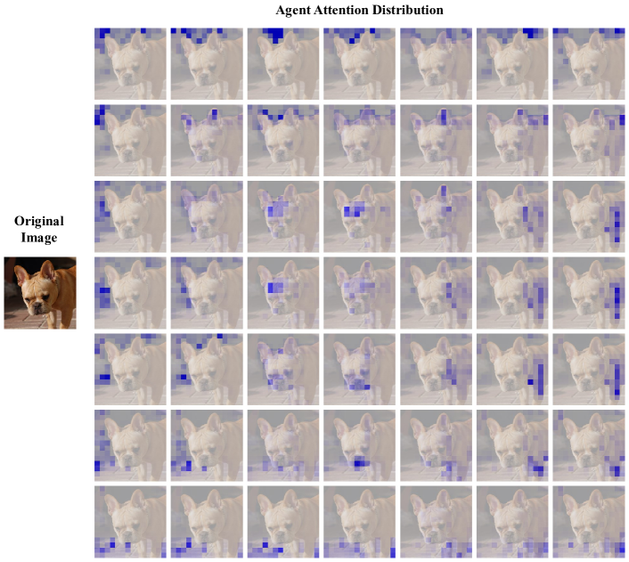
Figure 9: The distribution of attention weights corresponding to the 49 agent tokens from the third block of Agent-Swin-T.

C.3. ADE20K

Training settings. ADE20K [49] is a well-established benchmark for semantic segmentation which encompasses 20K training images and 2K validation images. Backbones are pretrained on ImageNet dataset with AdamW, following the training configurations mentioned in the original paper. For UperNet [42], we use AdamW to optimize, and set the initial learning rate as 6e-5 with a linear warmup of 1,500 iterations. Models are trained for 160K iterations in total. For Semantic FPN [20], we optimize the models using AdamW for 40k iterations with an initial learning rate of 2e-4. We randomly resize and crop the image to 512 × 512 for training, and re-scale to have a shorter side of 512 pixels during testing.

D. Complete Experimental Results

Full classification results. We provide the full ImageNet-1K classification results in Tab. 14. It is obvious that substituting Softmax attention with our agent attention in various models results in consistent performance improvements.

Additional downstream experiments. We provide additional experiment results on object detection and semantic segmentation in Tab.16, Tab.15 and Tab.17. For object detection, results on RetinaNet [23], Mask R-CNN [17] and Cascade Mask R-CNN [4] frameworks are presented, while for semantic segmentation, we show results on SemanticFPN [20] and UperNet [42]. It can be observed that our models achieve consistent improvements over their baseline counterparts across various settings.

E. Agent Attention Visualization

We visualize agent attention distribution in Fig. 9. It can be seen that various agent tokens focus on distinct regions, such as ears (second in the second row) and nose/mouth (fourth in the sixth row). This diversity ensures that different queries can focus on their areas of interest during the agent broadcast process.

F. Model Architectures

stage	output	Agent-DeiT-T		Agent-DeiT-S		Agent-DeiT-B
		Agent	DeiT Block	Agent	DeiT Block	Agent	DeiT Block
res1	$14\times 14$	$\left[\!\!\!\begin{array}[]{c}{\rm\ win}\ 14\!\times\!14\\ {\rm dim}\ 192\\ {\rm head}\ 3\\ {\rm agent}\ 49\end{array}\!\!\!\right]\!\!\times\!12$	None	$\left[\!\!\!\begin{array}[]{c}{\rm\ win}\ 14\!\times\!14\\ {\rm dim}\ 384\\ {\rm head}\ 6\\ {\rm agent}\ 49\end{array}\!\!\!\right]\!\!\times\!12$	None	$\left[\!\!\!\begin{array}[]{c}{\rm\ win}\ 14\!\times\!14\\ {\rm dim}\ 768\\ {\rm head}\ 12\\ {\rm agent}\ 81\end{array}\!\!\!\right]\!\!\times\!4$	$\left[\!\!\!\begin{array}[]{c}{\rm\ win}\ 14\!\times\!14\\ {\rm dim}\ 768\\ {\rm head}\ 12\end{array}\!\!\!\right]\!\!\times\!8$

Table 18: Architectures of FLatten-DeiT models.

stage	output	Agent-PVT-T		Agent-PVT-S
		Agent	PVT Block	Agent	PVT Block
res1	$56\times 56$	Conv1×1, stride=4, 64, LN
		$\left[\!\!\!\begin{array}[]{c}{\rm\ win}\ 56\!\times\!56\\ {\rm dim}\ 64\\ {\rm head}\ 1\\ {\rm agent}\ 9\end{array}\!\!\!\right]\!\!\times\!2$	None	$\left[\!\!\!\begin{array}[]{c}{\rm\ win}\ 56\!\times\!56\\ {\rm dim}\ 64\\ {\rm head}\ 1\\ {\rm agent}\ 9\end{array}\!\!\!\right]\!\!\times\!3$	None
res2	$28\times 28$	Conv1×1, stride=2, 128, LN
		$\left[\!\!\!\begin{array}[]{c}{\rm\ win}\ 28\!\times\!28\\ {\rm dim}\ 128\\ {\rm head}\ 2\\ {\rm agent}\ 16\end{array}\!\!\!\right]\!\!\times\!2$	None	$\left[\!\!\!\begin{array}[]{c}{\rm\ win}\ 28\!\times\!28\\ {\rm dim}\ 128\\ {\rm head}\ 2\\ {\rm agent}\ 16\end{array}\!\!\!\right]\!\!\times\!3$	None
res3	$14\times 14$	Conv1×1, stride=2, 320, LN
		$\left[\!\!\!\begin{array}[]{c}{\rm\ win}\ 14\!\times\!14\\ {\rm dim}\ 320\\ {\rm head}\ 5\\ {\rm agent}\ 49\end{array}\!\!\!\right]\!\!\times\!2$	None	$\left[\!\!\!\begin{array}[]{c}{\rm\ win}\ 14\!\times\!14\\ {\rm dim}\ 320\\ {\rm head}\ 5\\ {\rm agent}\ 49\end{array}\!\!\!\right]\!\!\times\!6$	None
res4	$7\times 7$	Conv1×1, stride=2, 512, LN
		$\left[\!\!\!\begin{array}[]{c}{\rm\ win}\ 7\!\times\!7\\ {\rm dim}\ 512\\ {\rm head}\ 8\\ {\rm agent}\ 49\end{array}\!\!\!\right]\!\!\times\!2$	None	$\left[\!\!\!\begin{array}[]{c}{\rm\ win}\ 7\!\times\!7\\ {\rm dim}\ 512\\ {\rm head}\ 8\\ {\rm agent}\ 49\end{array}\!\!\!\right]\!\!\times\!3$	None

Table 19: Architectures of Agent-PVT models (Part1).

stage	output	Agent-PVT-M		Agent-PVT-L
		Agent	PVT Block	Agent	PVT Block
res1	$56\times 56$	Conv1×1, stride=4, 64, LN
		$\left[\!\!\!\begin{array}[]{c}{\rm\ win}\ 56\!\times\!56\\ {\rm dim}\ 64\\ {\rm head}\ 1\\ {\rm agent}\ 9\end{array}\!\!\!\right]\!\!\times\!3$	None	$\left[\!\!\!\begin{array}[]{c}{\rm\ win}\ 56\!\times\!56\\ {\rm dim}\ 64\\ {\rm head}\ 1\\ {\rm agent}\ 9\end{array}\!\!\!\right]\!\!\times\!3$	None
res2	$28\times 28$	Conv1×1, stride=2, 128, LN
		$\left[\!\!\!\begin{array}[]{c}{\rm\ win}\ 28\!\times\!28\\ {\rm dim}\ 128\\ {\rm head}\ 2\\ {\rm agent}\ 16\end{array}\!\!\!\right]\!\!\times\!3$	None	$\left[\!\!\!\begin{array}[]{c}{\rm\ win}\ 28\!\times\!28\\ {\rm dim}\ 128\\ {\rm head}\ 2\\ {\rm agent}\ 16\end{array}\!\!\!\right]\!\!\times\!8$	None
res3	$14\times 14$	Conv1×1, stride=2, 320, LN
		$\left[\!\!\!\begin{array}[]{c}{\rm\ win}\ 14\!\times\!14\\ {\rm dim}\ 320\\ {\rm head}\ 5\\ {\rm agent}\ 49\end{array}\!\!\!\right]\!\!\times\!18$	None	$\left[\!\!\!\begin{array}[]{c}{\rm\ win}\ 14\!\times\!14\\ {\rm dim}\ 320\\ {\rm head}\ 5\\ {\rm agent}\ 49\end{array}\!\!\!\right]\!\!\times\!27$	None
res4	$7\times 7$	Conv1×1, stride=2, 512, LN
		$\left[\!\!\!\begin{array}[]{c}{\rm\ win}\ 7\!\times\!7\\ {\rm dim}\ 512\\ {\rm head}\ 8\\ {\rm agent}\ 49\end{array}\!\!\!\right]\!\!\times\!3$	None	$\left[\!\!\!\begin{array}[]{c}{\rm\ win}\ 7\!\times\!7\\ {\rm dim}\ 512\\ {\rm head}\ 8\\ {\rm agent}\ 49\end{array}\!\!\!\right]\!\!\times\!3$	None

Table 20: Architectures of Agent-PVT models (Part2).

stage	output	Agent-Swin-T		Agent-Swin-S		Agent-Swin-B
		Agent	Swin Block	Agent	Swin Block	Agent	Swin Block
res1	$56\times 56$	concat $4\times 4$, 96, LN		concat $4\times 4$, 96, LN		concat $4\times 4$, 128, LN
		$\left[\!\!\!\begin{array}[]{c}{\rm\ win}\ 56\!\times\!56\\ {\rm dim}\ 96\\ {\rm head}\ 3\\ {\rm agent}\ 9\end{array}\!\!\!\right]\!\!\times\!2$	None	$\left[\!\!\!\begin{array}[]{c}{\rm\ win}\ 56\!\times\!56\\ {\rm dim}\ 96\\ {\rm head}\ 3\\ {\rm agent}\ 9\end{array}\!\!\!\right]\!\!\times\!2$	None	$\left[\!\!\!\begin{array}[]{c}{\rm\ win}\ 56\!\times\!56\\ {\rm dim}\ 128\\ {\rm head}\ 3\\ {\rm agent}\ 9\end{array}\!\!\!\right]\!\!\times\!2$	None
res2	$28\times 28$	concat $4\times 4$, 192, LN		concat $4\times 4$, 192, LN		concat $4\times 4$, 256, LN
		$\left[\!\!\!\begin{array}[]{c}{\rm\ win}\ 28\!\times\!28\\ {\rm dim}\ 192\\ {\rm head}\ 6\\ {\rm agent}\ 16\end{array}\!\!\!\right]\!\!\times\!2$	None	$\left[\!\!\!\begin{array}[]{c}{\rm\ win}\ 28\!\times\!28\\ {\rm dim}\ 192\\ {\rm head}\ 6\\ {\rm agent}\ 16\end{array}\!\!\!\right]\!\!\times\!2$	None	$\left[\!\!\!\begin{array}[]{c}{\rm\ win}\ 28\!\times\!28\\ {\rm dim}\ 256\\ {\rm head}\ 6\\ {\rm agent}\ 16\end{array}\!\!\!\right]\!\!\times\!2$	None
res3	$14\times 14$	concat $4\times 4$, 384, LN		concat $4\times 4$, 384, LN		concat $4\times 4$, 512, LN
		None	$\left[\!\!\!\begin{array}[]{c}{\rm\ win}\ 7\!\times\!7\\ {\rm dim}\ 384\\ {\rm head}\ 12\end{array}\!\!\!\right]\!\!\times\!6$	None	$\left[\!\!\!\begin{array}[]{c}{\rm\ win}\ 7\!\times\!7\\ {\rm dim}\ 384\\ {\rm head}\ 12\end{array}\!\!\!\right]\!\!\times\!18$	$\left[\!\!\!\begin{array}[]{c}{\rm\ win}\ 14\!\times\!14\\ {\rm dim}\ 512\\ {\rm head}\ 12\\ {\rm agent}\ 49\end{array}\!\!\!\right]\!\!\times\!2$	$\left[\!\!\!\begin{array}[]{c}{\rm\ win}\ 7\!\times\!7\\ {\rm dim}\ 512\\ {\rm head}\ 12\end{array}\!\!\!\right]\!\!\times\!16$
res4	$7\times 7$	concat $4\times 4$, 768, LN		concat $4\times 4$, 768, LN		concat $4\times 4$, 1024, LN
		None	$\left[\!\!\!\begin{array}[]{c}{\rm\ win}\ 7\!\times\!7\\ {\rm dim}\ 768\\ {\rm head}\ 24\end{array}\!\!\!\right]\!\!\times\!2$	None	$\left[\!\!\!\begin{array}[]{c}{\rm\ win}\ 7\!\times\!7\\ {\rm dim}\ 768\\ {\rm head}\ 24\end{array}\!\!\!\right]\!\!\times\!2$	None	$\left[\!\!\!\begin{array}[]{c}{\rm\ win}\ 7\!\times\!7\\ {\rm dim}\ 1024\\ {\rm head}\ 24\end{array}\!\!\!\right]\!\!\times\!2$

Table 21: Architectures of Agent-Swin models.

stage	output	Agent-CSwin-T		Agent-CSwin-S		Agent-CSwin-B
		Agent	CSwin Block	Agent	CSwin Block	Agent	CSwin Block
res1	$56\times 56$	Conv7×7, stride=4, 64, LN				Conv7×7, stride=4, 96, LN
		$\left[\!\!\!\begin{array}[]{c}{\rm\ win}\ 56\!\times\!56\\ {\rm dim}\ 64\\ {\rm head}\ 2\\ {\rm agent}\ 9\end{array}\!\!\!\right]\!\!\times\!2$	None	$\left[\!\!\!\begin{array}[]{c}{\rm\ win}\ 56\!\times\!56\\ {\rm dim}\ 64\\ {\rm head}\ 2\\ {\rm agent}\ 9\end{array}\!\!\!\right]\!\!\times\!3$	None	$\left[\!\!\!\begin{array}[]{c}{\rm\ win}\ 56\!\times\!56\\ {\rm dim}\ 96\\ {\rm head}\ 4\\ {\rm agent}\ 9\end{array}\!\!\!\right]\!\!\times\!3$	None
res2	$28\times 28$	Conv7×7, stride=4, 128, LN				Conv7×7, stride=4, 192, LN
		$\left[\!\!\!\begin{array}[]{c}{\rm\ win}\ 28\!\times\!28\\ {\rm dim}\ 128\\ {\rm head}\ 4\\ {\rm agent}\ 16\end{array}\!\!\!\right]\!\!\times\!4$	None	$\left[\!\!\!\begin{array}[]{c}{\rm\ win}\ 28\!\times\!28\\ {\rm dim}\ 128\\ {\rm head}\ 4\\ {\rm agent}\ 16\end{array}\!\!\!\right]\!\!\times\!6$	None	$\left[\!\!\!\begin{array}[]{c}{\rm\ win}\ 28\!\times\!28\\ {\rm dim}\ 192\\ {\rm head}\ 8\\ {\rm agent}\ 16\end{array}\!\!\!\right]\!\!\times\!6$	None
res3	$14\times 14$	Conv7×7, stride=4, 256, LN				Conv7×7, stride=384, LN
		None	$\left[\!\!\!\begin{array}[]{c}{\rm\ win}\ 7\!\times\!14\\ {\rm dim}\ 256\\ {\rm head}\ 8\end{array}\!\!\!\right]\!\!\times\!18$	None	$\left[\!\!\!\begin{array}[]{c}{\rm\ win}\ 7\!\times\!14\\ {\rm dim}\ 256\\ {\rm head}\ 8\end{array}\!\!\!\right]\!\!\times\!29$	None	$\left[\!\!\!\begin{array}[]{c}{\rm\ win}\ 7\!\times\!14\\ {\rm dim}\ 384\\ {\rm head}\ 16\end{array}\!\!\!\right]\!\!\times\!29$
res4	$7\times 7$	Conv7×7, stride=4, 512, LN				Conv7×7, stride=4, 768, LN
		None	$\left[\!\!\!\begin{array}[]{c}{\rm\ win}\ 7\!\times\!7\\ {\rm dim}\ 512\\ {\rm head}\ 16\end{array}\!\!\!\right]\!\!\times\!1$	None	$\left[\!\!\!\begin{array}[]{c}{\rm\ win}\ 7\!\times\!7\\ {\rm dim}\ 512\\ {\rm head}\ 16\end{array}\!\!\!\right]\!\!\times\!2$	None	$\left[\!\!\!\begin{array}[]{c}{\rm\ win}\ 7\!\times\!7\\ {\rm dim}\ 768\\ {\rm head}\ 32\end{array}\!\!\!\right]\!\!\times\!2$

Table 22: Architectures of Agent-CSwin models.

We present the architectures of four Transformer models used in the main paper, including Agent-DeiT, Agent-PVT, Agent-Swin and Agent-CSwin in Tab.18-22. Considering the advantage of enlarged receptive field, we mainly replace Softmax attention blocks with our agent attention module at early stages of vision Transformer models.

References

- Bolya and Hoffman [2023] Daniel Bolya and Judy Hoffman. Token merging for fast stable diffusion. In CVPRW, 2023.
- Bolya et al. [2022] Daniel Bolya, Cheng-Yang Fu, Xiaoliang Dai, Peizhao Zhang, and Judy Hoffman. Hydra attention: Efficient attention with many heads. In ECCVW, 2022.
- Bolya et al. [2023] Daniel Bolya, Cheng-Yang Fu, Xiaoliang Dai, Peizhao Zhang, Christoph Feichtenhofer, and Judy Hoffman. Token merging: Your ViT but faster. In ICLR, 2023.
- Cai and Vasconcelos [2018] Zhaowei Cai and Nuno Vasconcelos. Cascade r-cnn: Delving into high quality object detection. In CVPR, 2018.
- Carion et al. [2020] Nicolas Carion, Francisco Massa, Gabriel Synnaeve, Nicolas Usunier, Alexander Kirillov, and Sergey Zagoruyko. End-to-end object detection with transformers. In ECCV, 2020.
- Cheng et al. [2021] Bowen Cheng, Alex Schwing, and Alexander Kirillov. Per-pixel classification is not all you need for semantic segmentation. In NeurIPS, 2021.
- Choromanski et al. [2021] Krzysztof Choromanski, Valerii Likhosherstov, David Dohan, Xingyou Song, Andreea Gane, Tamas Sarlos, Peter Hawkins, Jared Davis, Afroz Mohiuddin, Lukasz Kaiser, et al. Rethinking attention with performers. In ICLR, 2021.
- Cubuk et al. [2020] Ekin D Cubuk, Barret Zoph, Jonathon Shlens, and Quoc V Le. Randaugment: Practical automated data augmentation with a reduced search space. In CVPRW, 2020.
- Deng et al. [2009] Jia Deng, Wei Dong, Richard Socher, Li-Jia Li, Kai Li, and Li Fei-Fei. Imagenet: A large-scale hierarchical image database. In CVPR, 2009.
- Dettmers et al. [2022] Tim Dettmers, Mike Lewis, Sam Shleifer, and Luke Zettlemoyer. 8-bit optimizers via block-wise quantization. In ICLR, 2022.
- Dhariwal and Nichol [2021] Prafulla Dhariwal and Alexander Nichol. Diffusion models beat gans on image synthesis. In NeurIPS, 2021.
- Dong et al. [2022] Xiaoyi Dong, Jianmin Bao, Dongdong Chen, Weiming Zhang, Nenghai Yu, Lu Yuan, Dong Chen, and Baining Guo. Cswin transformer: A general vision transformer backbone with cross-shaped windows. In CVPR, 2022.
- Dosovitskiy et al. [2021] Alexey Dosovitskiy, Lucas Beyer, Alexander Kolesnikov, Dirk Weissenborn, Xiaohua Zhai, Thomas Unterthiner, Mostafa Dehghani, Matthias Minderer, Georg Heigold, Sylvain Gelly, et al. An image is worth 16x16 words: Transformers for image recognition at scale. In ICLR, 2021.
- Han et al. [2023a] Dongchen Han, Xuran Pan, Yizeng Han, Shiji Song, and Gao Huang. Flatten transformer: Vision transformer using focused linear attention. In ICCV, 2023a.
- Han et al. [2023b] Yizeng Han, Dongchen Han, Zeyu Liu, Yulin Wang, Xuran Pan, Yifan Pu, Chao Deng, Junlan Feng, Shiji Song, and Gao Huang. Dynamic perceiver for efficient visual recognition. In ICCV, 2023b.
- Hassani et al. [2023] Ali Hassani, Steven Walton, Jiachen Li, Shen Li, and Humphrey Shi. Neighborhood attention transformer. In CVPR, 2023.
- He et al. [2017] Kaiming He, Georgia Gkioxari, Piotr Dollár, and Ross Girshick. Mask r-cnn. In ICCV, 2017.
- Heusel et al. [2017] Martin Heusel, Hubert Ramsauer, Thomas Unterthiner, Bernhard Nessler, and Sepp Hochreiter. Gans trained by a two time-scale update rule converge to a local nash equilibrium. In NeurIPS, 2017.
- Katharopoulos et al. [2020] Angelos Katharopoulos, Apoorv Vyas, Nikolaos Pappas, and François Fleuret. Transformers are rnns: Fast autoregressive transformers with linear attention. In ICML, 2020.
- Kirillov et al. [2019] Alexander Kirillov, Ross Girshick, Kaiming He, and Piotr Dollár. Panoptic feature pyramid networks. In CVPR, 2019.
- Li et al. [2023] Yawei Li, Yuchen Fan, Xiaoyu Xiang, Denis Demandolx, Rakesh Ranjan, Radu Timofte, and Luc Van Gool. Efficient and explicit modelling of image hierarchies for image restoration. In CVPR, 2023.
- Lin et al. [2014] Tsung-Yi Lin, Michael Maire, Serge Belongie, James Hays, Pietro Perona, Deva Ramanan, Piotr Dollár, and C Lawrence Zitnick. Microsoft coco: Common objects in context. In ECCV, 2014.
- Lin et al. [2017] Tsung-Yi Lin, Priya Goyal, Ross Girshick, Kaiming He, and Piotr Dollár. Focal loss for dense object detection. In ICCV, 2017.
- Liu et al. [2022] Luping Liu, Yi Ren, Zhijie Lin, and Zhou Zhao. Pseudo numerical methods for diffusion models on manifolds. In ICLR, 2022.
- Liu et al. [2021] Ze Liu, Yutong Lin, Yue Cao, Han Hu, Yixuan Wei, Zheng Zhang, Stephen Lin, and Baining Guo. Swin transformer: Hierarchical vision transformer using shifted windows. In ICCV, 2021.
- Loshchilov and Hutter [2018] Ilya Loshchilov and Frank Hutter. Decoupled weight decay regularization. In ICLR, 2018.
- Lu et al. [2021] Jiachen Lu, Jinghan Yao, Junge Zhang, Xiatian Zhu, Hang Xu, Weiguo Gao, Chunjing Xu, Tao Xiang, and Li Zhang. Soft: Softmax-free transformer with linear complexity. In NeurIPS, 2021.
- Polyak and Juditsky [1992] Boris T Polyak and Anatoli B Juditsky. Acceleration of stochastic approximation by averaging. SIAM Journal on Control and Optimization, 1992.
- Radford et al. [2021] Alec Radford, Jong Wook Kim, Chris Hallacy, Aditya Ramesh, Gabriel Goh, Sandhini Agarwal, Girish Sastry, Amanda Askell, Pamela Mishkin, Jack Clark, Gretchen Krueger, and Ilya Sutskever. Learning transferable visual models from natural language supervision. In ICML, 2021.
- Rombach et al. [2022] Robin Rombach, Andreas Blattmann, Dominik Lorenz, Patrick Esser, and Björn Ommer. High-resolution image synthesis with latent diffusion models. In CVPR, 2022.
- Ruiz et al. [2023] Nataniel Ruiz, Yuanzhen Li, Varun Jampani, Yael Pritch, Michael Rubinstein, and Kfir Aberman. Dreambooth: Fine tuning text-to-image diffusion models for subject-driven generation. In CVPR, 2023.
- Seitzer [2020] Maximilian Seitzer. pytorch-fid: FID Score for PyTorch. https://github.com/mseitzer/pytorch-fid, 2020. Version 0.3.0.
- Shaw et al. [2018] Peter Shaw, Jakob Uszkoreit, and Ashish Vaswani. Self-attention with relative position representations. In ACL, 2018.
- Shen et al. [2021] Zhuoran Shen, Mingyuan Zhang, Haiyu Zhao, Shuai Yi, and Hongsheng Li. Efficient attention: Attention with linear complexities. In WACV, 2021.
- Song et al. [2021] Jiaming Song, Chenlin Meng, and Stefano Ermon. Denoising diffusion implicit models. In ICLR, 2021.
- Tan and Le [2019] Mingxing Tan and Quoc Le. Efficientnet: Rethinking model scaling for convolutional neural networks. In ICML, 2019.
- Touvron et al. [2021] Hugo Touvron, Matthieu Cord, Matthijs Douze, Francisco Massa, Alexandre Sablayrolles, and Hervé Jégou. Training data-efficient image transformers & distillation through attention. In ICML, 2021.
- Vaswani et al. [2017] Ashish Vaswani, Noam Shazeer, Niki Parmar, Jakob Uszkoreit, Llion Jones, Aidan N Gomez, Łukasz Kaiser, and Illia Polosukhin. Attention is all you need. In NeurIPS, 2017.
- Wang et al. [2021] Wenhai Wang, Enze Xie, Xiang Li, Deng-Ping Fan, Kaitao Song, Ding Liang, Tong Lu, Ping Luo, and Ling Shao. Pyramid vision transformer: A versatile backbone for dense prediction without convolutions. In ICCV, 2021.
- Wang et al. [2022] Wenhai Wang, Enze Xie, Xiang Li, Deng-Ping Fan, Kaitao Song, Ding Liang, Tong Lu, Ping Luo, and Ling Shao. Pvt v2: Improved baselines with pyramid vision transformer. Computational Visual Media, 2022.
- Xia et al. [2022] Zhuofan Xia, Xuran Pan, Shiji Song, Li Erran Li, and Gao Huang. Vision transformer with deformable attention. In CVPR, 2022.
- Xiao et al. [2018] Tete Xiao, Yingcheng Liu, Bolei Zhou, Yuning Jiang, and Jian Sun. Unified perceptual parsing for scene understanding. In ECCV, 2018.
- Xie et al. [2021] Enze Xie, Wenhai Wang, Zhiding Yu, Anima Anandkumar, Jose M Alvarez, and Ping Luo. Segformer: Simple and efficient design for semantic segmentation with transformers. In NeurIPS, 2021.
- Xiong et al. [2021] Yunyang Xiong, Zhanpeng Zeng, Rudrasis Chakraborty, Mingxing Tan, Glenn Fung, Yin Li, and Vikas Singh. Nyströmformer: A nyström-based algorithm for approximating self-attention. In AAAI, 2021.
- You et al. [2023] Haoran You, Yunyang Xiong, Xiaoliang Dai, Bichen Wu, Peizhao Zhang, Haoqi Fan, Peter Vajda, and Yingyan Celine Lin. Castling-vit: Compressing self-attention via switching towards linear-angular attention at vision transformer inference. In CVPR, 2023.
- Yun et al. [2019] Sangdoo Yun, Dongyoon Han, Seong Joon Oh, Sanghyuk Chun, Junsuk Choe, and Youngjoon Yoo. Cutmix: Regularization strategy to train strong classifiers with localizable features. In ICCV, 2019.
- Zhang et al. [2018] Hongyi Zhang, Moustapha Cisse, Yann N. Dauphin, and David Lopez-Paz. mixup: Beyond empirical risk minimization. In ICLR, 2018.
- Zhong et al. [2020] Zhun Zhong, Liang Zheng, Guoliang Kang, Shaozi Li, and Yi Yang. Random erasing data augmentation. In AAAI, 2020.
- Zhou et al. [2019] Bolei Zhou, Hang Zhao, Xavier Puig, Tete Xiao, Sanja Fidler, Adela Barriuso, and Antonio Torralba. Semantic understanding of scenes through the ade20k dataset. IJCV, 2019.
- Zhu et al. [2023] Lei Zhu, Xinjiang Wang, Zhanghan Ke, Wayne Zhang, and Rynson WH Lau. Biformer: Vision transformer with bi-level routing attention. In CVPR, 2023.