Block encoding of matrix product operators
Abstract
Quantum signal processing combined with quantum eigenvalue transformation has recently emerged as a unifying framework for several quantum algorithms. In its standard form, it consists of two separate routines: block encoding, which encodes a Hamiltonian in a larger unitary, and signal processing, which achieves an almost arbitrary polynomial transformation of such a Hamiltonian using rotation gates. The bottleneck of the entire operation is typically constituted by block encoding and, in recent years, several problem-specific techniques have been introduced to overcome this problem. Within this framework, we present a procedure to block-encode a Hamiltonian based on its matrix product operator (MPO) representation. More specifically, we encode every MPO tensor in a larger unitary of dimension , where is the number of subsequently contracted qubits that scales logarithmically with the virtual bond dimension . Given any system of size , our method requires ancillary qubits in total, while the computational cost for the decomposition of the block encoding circuit into one- and two-qubit gates scales as .
I Introduction
Quantum signal processing (QSP) combined with “qubitization” provides a unifying paradigm for several quantum algorithms [1, 2, 3]. The quantum eigenvalue transformation (QET) technique is part of this framework and facilitates a tailored polynomial transformation of the eigenvalues of a Hermitian matrix, which is typically a Hamiltonian of a quantum system of interest. QET has versatile applications, like eigenspace filtering, ground state preparation or Hamiltonian simulation.
In this whole process, the largest bottleneck is represented by the block encoding of . It is well known that a unitary operator embedding exists, but decomposing such a unitary efficiently into one- and two-qubit gates requires some extra knowledge of the system and problem-specific techniques. In this context, we propose a versatile block encoding method based on a matrix product operator (MPO) representation of , where such an MPO form is typically known or can be constructed for systems of interest. Our method uses unitary dilations of the individual MPO tensors. Our approach achieves a block encoding with computational cost scaling only linearly with the system size and quadratically with the virtual bond dimension of the MPO , while the number of ancillary qubits scales like the sum of and .
Our theoretical justification starts then in section II, where we provide a concise definition of MPOs within the context of tensor networks. This quick introduction is followed by the description of our algorithm in section III, which encodes such MPOs on a quantum computer. This task requires the use of ancillaries and measurements, as the MPO tensors are non-unitary in general.
We discuss the application of our method for QET in section IV. Specifically, we first outline a new method to implement the signal processing operator, which, in contrast to the one described by Martyn et al. [3], requires no auxiliary qubits and roughly half the number of gates. This technique is particularly suitable to be integrated with our MPO block encoding, as they can be partially executed in parallel, resulting in a reduction of the circuit depth. The theoretical proof of the correctness of this method is provided in appendix A
We then perform a cost analysis in terms of two-qubit gates count comparing our method to the linear combinations of unitaries (LCU) block encoding technique in section V. The results show that our technique is characterized by a scaling of , while the cost of LCU varies from polynomial to exponential, depending on the number of unitaries constituting the Hamiltonian.
Finally, we present some practical applications in section VI. We first examine the MPO representation of the Ising and Heisenberg Hamiltonians and then consider a general tensor product of sums of Paulis as an example exhibiting a significant advantage compared to the use of LCU. Within this last specific example, we finally realize the entire QET circuit simulating an eigenstate filtering process.
II Tensor networks and matrix product operators
We consider a physical system that can be represented as a 1D chain with sites. Then, a matrix product operator (MPO) is any operator acting on such a system as [4, 5]:
| (1) |
where every term is a matrix of operators acting on the -th site of the lattice except for the first and last term, which are respectively a row and column vector of operators. For the sake of concreteness, we will assume our MPO to have uniform virtual bond dimension and physical wires of dimension 2, where different cases are straightforward to generalize.
Figure 1a represents the tensor diagram of Eq. (1). In Fig. 1b, we defined the closing tensors and as the contraction between two tensors and of degree four, respectively with a row and column vector and . Such a manipulation of the closing tensors conveniently allows us to work with an MPO with uniform dimensions, while the role of the vectors and will be further investigated in sections IV and VI.
Such a decomposition can always be found through iterated singular values decompositions, exactly like matrix product states (MPS) [4]. However, this method quickly becomes computationally too expensive for increasing , so it is considered impracticable for most applications. Alternatively, it’s possible to build the MPO by representing the Hamiltonian through finite state automata [6, 7]. This method is particularly suitable for translation-invariant systems and in section VI we will show a few examples. From now on, we will assume that the MPO decomposition of the target Hamiltonian is known.
III Circuit representation
Now that the basic concepts for understanding matrix product operators have been introduced, we describe how to implement them on a quantum circuit. First of all, to make the tensors act on qubits as a quantum gate, we need to reshape them from four-tensors to matrices as shown below:
where we define as the matrix reshape of the tensor .
Given then the virtual bond dimension of the original MPO , which we assumed to be uniform, we proceed to expand the matrices so that their dimensions reach the next power of 2. Examples of this procedure will be shown in the applications section. Then, since we have postulated the physical wire to have dimension 2, we can assume to have dimensions , where is defined as:
| (2) |
It should be clear that if the physical wire can be represented with one single qubit, the virtual bond needs qubits. From now on, we will refer to the latter as virtual bond ancillaries.
The last step needed to represent as a quantum circuit is a unitary dilation, i.e., we embed each as a block in a larger unitary matrix. This procedure will require another ancillary qubit, which we will refer to as dilation ancillary. From a diagrammatic point of view, and after reshaping back the unitary matrices in tensors of degree 4, we get the final MPO form as in Fig. 1c, where each green wire corresponds to one physical qubit, each red wire has the role of dilation ancillary and the blue dashed wires represent the virtual bond ancillaries.
Using one ancillary qubit has the effect of doubling the size of the encoding unitaries: more specifically, we want to define a unitary matrix so that its upper-left block is equal to up to a normalization factor :
| (3) |
We denote such unitaries as block encodings of the matrices . Note that the normalization factor is necessary because are typically not normalized and is characterized by the relation:
| (4) |
with denoting the spectral norm. Our aim now is to find the blocks , and so that, given , is unitary. To do that, we rely on a similar procedure as proposed in [8, Appendix D].
-
1.
From the unitary constraint on it follows that
(5) Let us consider then the singular value decomposition of the matrix :
(6) with and unitary matrices and the diagonal matrix of singular values.
-
2.
Let us consider now the following rectangular matrix:
(9) where has been found through the previous step. A full QR decomposition applied to returns a unitary matrix and a rectangular, upper triangular matrix so that
(10) In the first half of its columns, will share the same entries as , since they were already orthonormal; as a result, the unitary matrix is of the form (3), so that we can set .
Now that we have achieved a unitary block encoding for each , we can represent the entire MPO tensor network by a quantum circuit. Fig. 2 shows the full block encoding circuit for a generic Hamiltonian acting on a system of size as an example. Note that:
-
•
The block encoding circuit needs in total physical qubits, marked in green, virtual bond ancillaries, blue dashed, and dilation ancillaries, marked in red. The total number of ancillaries is then , and the color scheme matches the one for the equivalent wires of the tensor networks in Fig 1.
-
•
To retrieve the Hamiltonian , the dilation ancillaries must be all initialized and measured in the state . The virtual bond ancillaries must also be prepared in state and measured in state , representing the column and row vectors and previously defined. As a result, a post-selection operation is needed to fully implement on a quantum circuit. Some further discussions about this topic, including an idea on how to do that in practice, can be found in section IV.
-
•
The cost for decomposing each into one- and two-qubit gates drastically varies for different applications and different native gate sets of the specific hardware. Nonetheless, in the most general case, it grows exponentially with the number of wires involved in each gate, equal to , so that the number of two-qubit gates scales as [9, 10]. Returning to the virtual bond dimension formalism and recalling Eq. (2), we can conclude that the computational cost for the MPO circuit scales linearly with the system size and quadratically with the virtual bond dimension as .
IV Quantum eigenvalue transformation with MPO block encoding
We now illustrate the quantum eigenvalue transformation (QET) algorithm [3] as a possible application of our block encoding method.
Given a block encoding of a Hamiltonian and a polynomial of degree , there exists a sequence of angles so that (in the case of even):
| (11) |
The signal processing operators are defined as:
| (12) |
where is the projector onto : . Similarly, for odd , Eq. (11) becomes:
| (13) |
In the previous sections, we have illustrated how to create a unitary encoding for an MPO Hamiltonian acting on sites through ancillary qubits. The next step consists of specifying the signal processing operator .
To retrieve the Hamiltonian from the block encoding depicted in Fig. 2, we need to project onto for all the red wires (both initialization and measurement), and for the virtual bond ancillaries, we need to initialize the state and measure . For the sake of simplicity, we make use of the two state-preparation gates and :
| (14) | ||||
| (15) |
to initialize and measure the virtual bond ancillaries in the state , just like the dilation ancillaries. The overall QET circuit, before specifying how to build the signal processing operator, is visualized in Fig. 3.
Martyn et al.’s paper [3] contains a first proposal for building the operator with one extra auxiliary qubit. As an example, the mentioned operator would be implemented in the following way for and :
| (16) |
Note that we always need exactly one extra auxiliary qubit (in yellow) and the signal processing gate acts on all the dilation and virtual bond ancillaries.
Here we propose a different approach to implement using multi-controlled -rotations, instead of multi-controlled NOTs, and no extra auxiliary qubit. For the same example as in Eq. (16), the circuit reads (see Appendix A for a derivation):
| (17) |
where the -th gate is controlled by qubits and the corresponding -rotation has phase .
Note that, in order to decompose each multi-controlled rotation into one- and two-qubit gates, we can make use of the following relation [11, 12]:
| (18) |
until we get solely single-qubit -rotation gates, all with the same phase , and CNOTs. Some of the latter cancel out in the overall circuit [11] and the final CNOT count is exactly . Note that the circuit in Eq. (16) requires one additional control qubit. Its decomposition, using similar techniques, would then require CNOTs. Consequently, our method offers roughly a factor 2 reduction in CNOT count.
Moreover, given the cascading shape of our MPO block encoding, part of the signal processing circuit can be executed in parallel with the block encoding with a further reduction of the circuit’s depth, as illustrated in Fig. 4. Given then the interchangeability of the ancillaries from the signal processing point of view, we can invert the order of the controlled rotations and start from the bottom wire up, so that also can be partially executed in parallel with the following .
V Cost Analysis
Before illustrating some possible applications, we would like to discuss the cost of a general QET circuit built with our block encoding algorithm, in comparison to the linear combination of unitaries (LCU) technique [13, 2, 14] shown in Fig. 5. More specifically, we evaluate the computational cost based on the count of one- and two-qubit gates.
The LCU method is based on the insight that every Hamiltonian can be written as a linear combination of unitaries:
| (19) |
For concreteness, we will consider the case where all the are Pauli strings. The total number of terms in the summation is denoted as . In the worst case scenario, scales exponentially with the system size as . Still, there are important examples of polynomial or even linear scaling, like the Ising or Heisenberg Hamiltonian. We will first discuss the general case and then return to the specific examples later.
For LCU, one first adds ancillary qubits to the circuit that need to be prepared in the state:
| (20) |
with the same coefficients as in Eq. (19). This preparation gate, as well as any other multi-qubit controlled gate that we will consider in this section, must be decomposed into one- and two-qubit gates. Generally speaking, this process has a cost that scales exponentially with the number of qubits squared [9, 10], which means .
The next step is known as the selection phase: here each state controls one of the unitaries . We have therefore Pauli strings acting on the system qubits and controlled by the ancillary qubits. Supposing that each Pauli gate can be implemented with a constant cost on a quantum computer, we get gates for each , while the multi-control can be decomposed with a cost exponential in the number of ancillaries and thus linear in . As a consequence, the cost of the decomposition for the full selection phase scales as . As a last step, we need to apply the inverse preparation gate on the ancillaries, with a final cost of .
Summarizing, the overall cost of LCU including a decomposition into single- and two-qubit gates scales as .
In the worst case, with scaling as , we get then ancillary qubits and a total cost of gates.
On the other hand, if we consider the case of linear scaling, we get a total cost for the decomposition of with ancillaries. It’s worth noticing that the aforementioned Ising and Heisenberg Hamiltonians fall under this scenario, since they are defined as a linear sum of Pauli strings. However, because of the nearest-neighbor constraint, they can get an even better scaling of , as the Pauli strings are only composed by one or two Pauli gates.
Regarding our MPO block encoding, we will only consider its worst-case scenario. The resulting circuit shown in Fig. 2 is implemented through unitaries acting each on wires: decomposing them requires then a cost of at most. The preparation gates and do not change the formal complexity, as they scale at most as . In conclusion, we can state that we always get a linear dependence on the system size and a quadratic scaling with the virtual bond dimension . It is also worth recalling that the number of ancillary qubits is precisely equal to .
| Ancillary qubits | Block encoding cost | Signal processing cost | |
| MPO Block Encoding | |||
| LCU Block Encoding | |||
| LCU Block Encoding | |||
| LCU Block Encoding |
Table 1 summarizes the MPO and LCU block encoding costs, the latter with specific examples of scaling exponentially or linearly with . We also added the signal processing decomposition cost, which scales exponentially with the number of ancillary qubits, as discussed in the previous paragraphs.
Note that for LCU, the block encoding cost always exceeds the signal processing cost. For our MPO block encoding, however, we notice the opposite effect. Given the linear scaling with and the quadratic dependence on , our block encoding turns out to be competitive compared to LCU. If we consider, for example, the aforementioned Ising and Heisenberg models, the corresponding MPO block encoding only scales linearly with since is constant, as it will be further discussed in section VI. On the other hand, the relatively large number of ancillary qubits, on which the signal processing scales exponentially, makes the signal processing more expensive.
In conclusion, when considering the block encoding by itself, our MPO method can have a lower computational cost than LCU in certain situations. The signal processing phase contributes the most to the MPO method when considering the whole QET circuit. It is also worth mentioning that this analysis is based on the current technologies not allowing three-qubit gates or more, and that future hardware developments might revise this analysis.
VI Applications
This section demonstrates how our block encoding technique can be applied to specific Hamiltonians. As a first example, we consider the Ising and Heisenberg Hamiltonians, which have a relatively simple MPO representation.
Then, we consider the case where a sum of Pauli strings can be rearranged in a tensor product of sums of local Pauli operators. For this system, we get an extremely simple MPO representation and a practical advantage compared to LCU. We also chose this system to perform an eigenstate filtering procedure through an entire QET circuit.
VI.1 Ising model with transverse field
The Ising Hamiltonian with transverse field is defined as follows:
| (21) |
with and Pauli operators acting on the -th site. Then, a suitable MPO decomposition can be achieved by defining the internal tensors as [16, 6]:
| (22a) | ||||
| and by “closing” the tensor chain with the following initial and final vectors of operators, respectively: | ||||
| (22b) | ||||
| (22c) | ||||
Every local operator acts on the -th lattice site, and is the identity matrix. Such a representation can be easily found through a finite state automata picture of the Hamiltonian, as shown in [6, 13].
One can also verify that the closing vectors can be obtained via:
| (23a) | ||||
| (23b) | ||||
with and defined as the other . Eq. (1) for the Ising model then becomes:
| (24) |
We immediately notice that since the Pauli operators act on single qubits, and have dimension , each matrix has dimension and therefore needs at least 3 qubits to be represented. As a consequence, all the matrices and vectors in Eq. (24) gain a new row and/or column in the following way:
| (25a) | ||||
| (25b) | ||||
| (25c) | ||||
The state-preparation gates and are the identity operator and , respectively.
Among the qubits that represent each matrix , only one has the role of physical qubit (different for every tensor), while the other are subsequently contracted. Moreover, the meaning of the column and row vectors and is now clearer, as they correspond to the initialization of the virtual bond ancillaries in the state and their projection after measurement in the state .
Note that to construct a block encoding of , we have to normalize it by a factor . This has the same effect as dividing the Hamiltonian parameters and by :
| (26a) | ||||
| (26b) | ||||
It is worth mentioning that some algorithms, including the eigenstate filtering process that we have applied to the tensor product of Pauli sums, require the eigenvalues of not only to have an absolute value smaller than , but also to be positive. To achieve that, one may add an extra auxiliary qubit and control the entire block encoding process as shown in Fig. 6 [3]. Within our specific technique, however, we can add a term to Eq. (21) without any extra computational cost by simply changing the MPO definition and initial and final projections:
| (27a) | ||||
| (27b) | ||||
| (27c) | ||||
As a consequence, the state preparation operators become:
| (28a) | ||||
| (28b) | ||||
Note that, when normalizing the Hamiltonian, we also need to consider an extra factor given by the normalization of states and , so that:
| (29a) | ||||
| (29b) | ||||
In the specific Ising case, we can thus shift the eigenvalues of in the interval without a significant increase in the computational cost. In other cases, however, adding a new identity operator in the right-bottom corner of could increase the dimension beyond , requiring one additional virtual bond ancillary.
VI.2 Heisenberg model
Next, we discuss the Heisenberg model governed by the Hamiltonian
| (30) |
It can be proven that the corresponding MPO decomposition has a similar structure as for the Ising model with matrices [17, 6]:
| (31) |
The matrix in Eq. (31) has dimension and therefore needs to be expanded into a matrix (analogous to the Ising MPO model) to be represented by qubits. Moreover, another dilation ancillary is added to build through a QR decomposition.
As a result, the entire block encoding circuit resembles the Ising example but with virtual bond ancillaries instead of , given the larger dimensions of ; the latter needs then to be initialized in the state and measured in the state .
The XY model, which restricts the more general Heisenberg model to the XY plane, is particularly interesting. Removing the rows and columns containing results in an MPO matrix of dimensions , which can be represented with 3 qubits and no further expansion. Thus, the XY model requires the same computational resources as the Ising model.
VI.3 Tensor product of sum of Paulis
Finally, we consider a different Hamiltonian, for which our block encoding technique offers a significant advantage compared to LCU; we also test the entire QET algorithm by applying an eigenstate filtering transformation to such a Hamiltonian. Let us consider the particular case of a tensor product of sums of local Pauli matrices:
| (32) |
The MPO representation is straightforward, as each MPO tensor is a one-qubit matrix:
| (33) |
with virtual bond ancillaries.
Following the eigenstate filtering process from Martyn et al.’s paper [3], we learn that the Hamiltonian should only have positive eigenvalues. By following a similar strategy as discussed for the Ising model, we add an element to ; the tensors are then modified in the following way:
| (34) |
so that each requires now two qubits to be represented, one physical and one constituting the virtual bond ancillary, plus the dilation ancillary. The virtual bond ancillary must then be initialized and measured in the state so that:
| (35) |
which lets us identify both preparation gates and with a Hadamard gate. Note that the coefficients and have been redefined in order to absorb the factor 2 derived by the two Hadamard transformations and the normalization factors that make for every . Different from the Ising and Heisenberg models, we do not assume translation invariance here. This means that each typically varies, as well as its norm, and in theory, one could choose one large enough to normalize all tensors as well as a different factor for each .
For comparison, if we wanted to block-encode Eq. (32) through the LCU method, we could exploit the tensor product structure and encode each of the terms separately. This way, for every physical qubit we would need ancillaries, prepared for example in the state:
| (36) |
so that each two-qubit state controls only the corresponding Pauli acting on the physical qubit. If we wanted then to shift the eigenvalues in the range we could exploit the trick in Fig. 6, which roughly doubles the computational cost of the entire circuit but does not change the formal complexity.
Regarding the formal computational complexity, both block encoding techniques scale linearly with in gate count and ancillary qubits. However, the exact number of ancillaries differs: the LCU method requires ancillaries while the MPO method requires . This means that we get a better scaling for the signal processing part, as the latter scales exponentially with the number of ancillary qubits.
VI.4 Eigenstate filtering
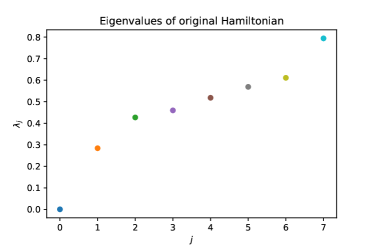
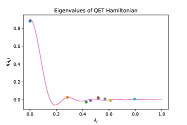
Finally, we test our block encoding algorithm, as well as our signal processing technique, by applying an eigenstate filtering function to the Hamiltonian defined in (32). In particular, we want to perform the following transformation over [18]:
| (37) |
where is the gap between the first and second eigenvalue and is the Chebyshev polynomial of order . Using the Python package pyqsp [3], we have been able to get the angles better approximating the function through a QET. In figure 7 one can then see a specific example with the Hamiltonian’s initial eigenvalues as well as their final values after the entire QET circuit compared with the target filtering function.
pyqsp was built for working with quantum signal processing and for acting on a specific one-qubit signal operator, which differs slightly from the conventions that we have used. Still, it is possible to adapt pyqsp’s angles for our purposes by following the instructions in Appendix A.2 of [3].
Moreover, a QET process with these phases generates a complex polynomial transformation, whose real part is our target function. When simulating the circuit, it is therefore necessary to take the hermitian part of the final outcome to get the desired result:
| (38) |
Such a combination of and cannot be directly performed on a quantum computer. For simplicity, we leave the question of how to perform this operation on a quantum computer for future work. To demonstrate the working of the algorithm, we have evaluated it classically.
VII Conclusion
Our block encoding method is generally applicable, since every Hamiltonian can be decomposed in a matrix product operator. Moreover, for every Hamiltonian and corresponding MPO representation, our block encoding technique’s computational cost grows only linearly with the system size and quadratically with the virtual bond dimension, offering a potential advantage with respect to LCU in terms of one- and two-qubit gates. In section VI we have shown one specific example of computational advantage in the case of a Hamiltonian equal to the tensor product of sums of local Pauli gates.
The scaling of the ancillary qubits, however, limits our algorithm’s speed-up. The signal processing operator is indeed composed of multi-controlled gates acting on the ancillaries, meaning that, with the current technologies, it incurs a cost growing exponentially with the number of ancillaries. Hypothetically, with further technological developments both in the hardware and quantum gates decomposing techniques, we might need to reconsider our cost analysis with potentially greater advantages.
A possible future project might focus on generalizing our protocol to Hamiltonians defined on two-dimensional lattices and their projected entangled-pair operator representation, inspired by isometric tensor networks [19] to construct the unitary dilations. This is particularly promising since the qubit topologies of modern quantum computers are often likewise two-dimensional grids.
As previously mentioned, each matrix encoded into a larger unitary must have a bounded norm. Encoding directly in a larger unitary, or using LCU, requires . In our case, we need to normalize each tensor individually, causing an equivalent rescaling of the Hamiltonian by a factor . The required renormalization is a general issue of block encoding and is not specific to our MPO approach, but the spectral norm of the individual matrices is typically easier to calculate than , which gives another practical advantage in using our method.
Finally, we would like to recall that since a post-processing selection is needed for both the Hamiltonian representation and the QET circuit, it would be advisable to conduct a further investigation into the success probability of these measurements. Our work should therefore be considered as an introductory paper presenting a new and promising technique, which will need to be further studied in the future.
Acknowledgements
M. Nibbi acknowledges funding by the Munich Quantum Valley, section K5 Q-DESSI. The research is part of the Munich Quantum Valley, which is supported by the Bavarian state government with funds from the Hightech Agenda Bayern Plus.
Appendix A Signal processing circuit
In this section, we prove that the circuits drawn in Eqs. (17) and (18) are equivalent. First of all, we recall the definition of the signal processing operator in Eq. (12). Without loss of generality, we can consider the case in which , where is the total number of ancillary qubits.
The matrix form of is:
| (39) |
It follows directly that Eq. (17) holds, since the state is the only one that gains a phase , while the other states acquire the phase .
The general form of our signal processing circuit, without distinguishing between dilation and virtual bond ancillaries, equals:
| (40) |
Let us consider the -th operator in the circuit (40). This operator has controls and a rotation phase of . Its matrix expression, considering the tensor multiplication with identities as well, is:
| (41) |
By multiplying all the matrices (41) with from 1 to , we get then the following:
| (42) |
Apart from the first entry, we can consider separate diagonal blocks. Taking , the -th block has dimension and entries equal to . We want to prove that each one of these does not depend on and, more specifically, is equal to :
| (43) |
The first block, on the other hand, has the following entry:
| (44) |
References
- Gilyén et al. [2019] A. Gilyén, Y. Su, G. H. Low, and N. Wiebe, Quantum singular value transformation and beyond: exponential improvements for quantum matrix arithmetics, in Proceedings of the 51st Annual ACM SIGACT Symposium on Theory of Computing, STOC 2019 (Association for Computing Machinery, 2019) pp. 193–204.
- Low and Chuang [2019] G. H. Low and I. L. Chuang, Hamiltonian simulation by qubitization, Quantum 3, 163 (2019).
- Martyn et al. [2021] J. M. Martyn, Z. M. Rossi, A. K. Tan, and I. L. Chuang, Grand unification of quantum algorithms, PRX Quantum 2, 040203 (2021).
- Schollwöck [2011] U. Schollwöck, The density-matrix renormalization group in the age of matrix product states, Ann. Physics 326, 96 (2011).
- Zaletel et al. [2015] M. P. Zaletel, R. S. K. Mong, C. Karrasch, J. E. Moore, and F. Pollmann, Time-evolving a matrix product state with long-ranged interactions, Phys Rev. B 91, 165112 (2015).
- Fröwis et al. [2010] F. Fröwis, V. Nebendahl, and W. Dür, Tensor operators: Constructions and applications for long-range interaction systems, Phys. Rev. A 81, 10.1103/physreva.81.062337 (2010).
- Crosswhite et al. [2008] G. M. Crosswhite, A. C. Doherty, and G. Vidal, Applying matrix product operators to model systems with long-range interactions, Phys. Rev. B 78, 10.1103/physrevb.78.035116 (2008).
- Lin et al. [2021] S.-H. Lin, R. Dilip, A. G. Green, A. Smith, and F. Pollmann, Real- and imaginary-time evolution with compressed quantum circuits, PRX Quantum 2, 010342 (2021).
- Krol et al. [2021] A. M. Krol, A. Sarkar, I. Ashraf, Z. Al-Ars, and K. Bertels, Efficient decomposition of unitary matrices in quantum circuit compilers, arXiv:2101.02993 (2021), arXiv:2101.02993 [quant-ph] .
- Rakyta and Zimborás [2022] P. Rakyta and Z. Zimborás, Approaching the theoretical limit in quantum gate decomposition, Quantum 6, 710 (2022).
- Shende et al. [2006] V. V. Shende, S. S. Bullock, and I. L. Markov, Synthesis of quantum-logic circuits, IEEE Transactions on Computer-Aided Design of Integrated Circuits and Systems 25, 1000 (2006).
- Möttönen et al. [2004] M. Möttönen, J. J. Vartiainen, V. Bergholm, and M. M. Salomaa, Quantum circuits for general multiqubit gates, Phys. Rev. Lett. 93, 130502 (2004).
- Childs and Wiebe [2012] A. M. Childs and N. Wiebe, Hamiltonian simulation using linear combinations of unitary operations, Quant. Inf. Comput. 12, 0901 (2012).
- Berry et al. [2015] D. W. Berry, A. M. Childs, R. Cleve, R. Kothari, and R. D. Somma, Simulating Hamiltonian dynamics with a truncated Taylor series, Phys. Rev. Lett. 114, 090502 (2015).
- Barenco et al. [1995] A. Barenco, C. H. Bennett, R. Cleve, D. P. DiVincenzo, N. Margolus, P. Shor, T. Sleator, J. A. Smolin, and H. Weinfurter, Elementary gates for quantum computation, Phys. Rev. A 52, 3457 (1995).
- Ran et al. [2020] S.-J. Ran, E. Tirrito, C. Peng, X. Chen, L. T. G. Su, and M. Lewenstein, Tensor network contractions - Methods and applications to quantum many-body systems, Title Lecture Notes in Physics (Springer Cham, 2020).
- Yamada and Fukai [2023] K. Yamada and K. Fukai, Matrix product operator representations for the local conserved quantities of the Heisenberg chain, arXiv:2306.03431 (2023), arXiv:2306.03431 [cond-mat.stat-mech] .
- Lin and Tong [2020] L. Lin and Y. Tong, Optimal polynomial based quantum eigenstate filtering with application to solving quantum linear systems, Quantum 4, 361 (2020).
- Zaletel and Pollmann [2020] M. P. Zaletel and F. Pollmann, Isometric tensor network states in two dimensions, Phys. Rev. Lett. 124, 037201 (2020).