Safe data-driven reference tracking with prescribed performance

Abstract

We study output reference tracking for unknown continuous-time systems with arbitrary relative degree. The control objective is to keep the tracking error within predefined time-varying bounds while measurement data is only available at discrete sampling times. To achieve the control objective, we propose a two-component controller. One part is a recently developed sampled-data zero-order hold controller, which achieves reference tracking within prescribed error bounds. To further improve the control signal, we explore the system dynamics via input-output data, and include as the second component a data-driven MPC scheme based on Willems et al.’s fundamental lemma. This combination yields significantly improved input signals as illustrated by a numerical example.

I Introduction

We study output-reference tracking of unknown continuous-time linear systems with arbitrary relative degree, where the output measurement data is only available at discrete sampling times. The control task is to ensure that the tracking error evolves strictly within predefined time-varying bounds. The latter aspect is subject of various results in feedback control, such as prescribed performance control [1], see also [2] for a comprehensive literature review; or funnel control [3], cf. [4] for an extensive literature overview. Since sampled-data control is closely related to digital control, there is plenty of literature available. In the current context we may pick out [5, 6], where stabilization of linear systems via sampled-data state feedback is studied, and [7], where $H_{\infty}$ performance guarantee is achieved by quantized feedback.

Recently, a Zero-order Hold (ZoH) output-feedback controller was proposed [8], which achieves reference tracking at the output of an unidentified non-linear system with error guarantees, while only receiving measurement data at discrete sampling times. However, since only structural assumptions are invoked, the controller relies on worst-case estimations and exhibit a potentially unnecessarily large (and heavily oscillating) control signal, which is not desirable. In this article, we aim to improve the controller performance of the ZoH controller [8] by combining it with a data-driven Model Predictive Control (MPC) approach. The latter is based on the results found by Willems and coauthors in [9], now known as Willems et al.’s fundamental lemma. This result allows the description of an unknown discrete-time linear time-invariant system in a non-parametric fashion. The finite-length input-output trajectories of the system lie in the column space of a suitable Hankel matrix constructed directly from measured data. Based on this non-parametric description, it is possible to develop an MPC scheme that uses only input-output data instead of an a priori given model, cf. [10, 11, 12]. The fundamental lemma is subject to recent substantial research in the field of data-driven control. In [13, 14, 15], it was extended to stochastic descriptor systems. Extensions towards continuous-time and non-linear systems can be found, e.g., in [16, 17, 18] and [19, 20] resp. For a broader overview, we refer the reader to [21] and [14].

The contribution of the present article is an application of data-based MPC to improve the controller performance for an unknown linear system, while guaranteeing pre-specified time-varying error bounds on the tracking error. We partition the set of feasible outputs into a safe and a safety-critical region. In the safe region, we generate persistently-exciting input signals to explore the system behaviour and, then, set up a learning-based predictive controller (exploitation). In the safety-critical region, we resort to the recently proposed controller [8] to steer the system into the safe region. The basic idea is reminiscent of [22] and follow-up work [23], where safe and unsafe operating regions were used for economic MPC. In comparison to [8], we drastically reduce peaks in the control signal. Further, we show that the prediction horizon within the MPC scheme can be adaptively and freely chosen without jeopardizing (recursive) feasibility and the guaranteed trajectory tracking within the pre-specified error bounds in comparison to existing work, see, e.g., [24, 25, 26, 27, 28].

The restriction to linear systems in our presentation is merely of exemplary nature. We emphasize, that for the proposed controller we may also allow for nonlinear continuous-time systems, cf. [8]. In this case the guaranties on the tracking performance are still valid, even though the significance of the data-based linear surrogate model used in the MPC scheme and, therefore, the quality of the control signal are uncertain. Here, for instance, the mentioned extensions of the fundamental lemma for nonlinear systems have the potential of improving the controller.

This paper is structured in the following way. In Section II we introduce the examined system class and formulate the control objective. In Section III we present the controller and its components. To this end, we recap Willems et al.’s fundamental lemma and its leverage in data-driven MPC. Subsequently, we recall the theoretical foundation for the ZoH component. Then, an algorithmic implementation of the two-component controller is proposed. In Section IV the main result is presented and in Section V a numerical example is provided to illustrate the controller performance.

Notation: Let $\mathds{R}_{\geq 0}:=[0,\infty)$. For $x\in\mathds{R}^{n}$, the Euclidean norm is denoted by $\left\|x\right\|$ and ${\left\|x\right\|}_{Q}:=\sqrt{x^{\top}Qx}$ denotes the norm induced by a symmetric positive definite matrix $Q\in\mathbb{R}^{n\times n}$. For $p\in\mathds{N}_{0}\cup\{\infty\}$ the space of $p$-times continuously differentiable functions on $V\subset\mathds{R}^{m}$ with image in $\mathds{R}^{n}$ is denoted by $\mathcal{C}^{p}(V,\mathds{R}^{n})$ and $\mathcal{C}(V,\mathds{R}^{n}):=\mathcal{C}^{0}(V,\mathds{R}^{n})$. Let $L^{\infty}(I,\mathds{R}^{n})$ be the space of measurable essentially bounded functions from an interval $I\subset\mathds{R}$ into $\mathds{R}^{n}$, equipped with the usual norm $\left\|\cdot\right\|_{\infty}$. $L^{\infty}_{\text{loc}}(I,\mathds{R}^{n})$ is the space of locally-bounded measurable functions. $W^{k,\infty}(I,\mathds{R}^{n})$ is the $k$th-order Sobolev space with respect to $L^{\infty}(I,\mathds{R}^{n})$. For a finite sequence $(f_{k})_{k=0}^{N-1}$ in $\mathbb{R}^{n}$ of length $N$ we define the vectorization $f_{[0,N-1]}:=\begin{bmatrix}f_{0}^{\top}&\dots&f_{N-1}^{\top}\end{bmatrix}{}^{\top}\in\mathbb{R}^{nN}$. $\text{GL}_{m}(\mathds{R})$ denotes the group of invertible $(m\times m)$ matrices.

II Problem formulation

In this section, we introduce the considered system class and formulate the control objective.

II-A System class

We consider linear time-invariant control systems

$$\dot{x}(t) =Ax(t)+Bu(t),\qquad x(0)=x^{0},$$ (1)

$$y(t) =Cx(t),$$

where $x(t)\in\mathds{R}^{n}$ is the state at time $t\geq 0$, $A\in\mathds{R}^{n\times n}$ is the drift dynamics, $B\in\mathds{R}^{n\times m}$ is the input distribution matrix, and $C\in\mathds{R}^{m\times n}$ defines the output matrix. Note that input $u(t)$ and output $y(t)$ are of the same dimension $m\in\mathds{N}$. We make the following assumptions.

Assumption 1.

System (1) has strict relative degree $r\in\mathds{N}$:

$$\forall\,k=0,\ldots,r-2:\,CA^{k}B=0,\text{ and }CA^{r-1}B\in\text{GL}_{m}(\mathds{R}).$$

Assumption 1 allows us to find a linear coordinate transformation $U\in\text{GL}_{n}(\mathds{R})$ such that $Ux=(y,\dot{y},\ldots,y^{(r-1)},\eta)$ represents system (1) in the so-called Byrnes-Isidori form [29]

$$y^{(r)}(t) =\sum_{i=0}^{r-1}L_{i}y^{(i)}(t)+S\eta(t)+\Gamma u(t),$$ (2a)

$$\dot{\eta}(t) =K\eta(t)+Py(t),$$ (2b)

where $(y(0),\dot{y}(0),\ldots y^{(r-1)}(0),\eta(0))=Ux^{0}$, and for $i=0,\ldots,r-1$ we have $L_{i}\in\mathds{R}^{m\times m}$, $S,P^{\top}\in\mathds{R}^{m\times(n-rm)}$, $K\in\mathds{R}^{(n-rm)\times(n-rm)}$, and $\Gamma:=CA^{r-1}B\in\text{GL}_{m}(\mathds{R})$ is the so-called high-gain matrix. The latter is specified in the next assumption.

Assumption 2.

The high-gain matrix $\Gamma=CA^{r-1}B$ has strictly positive definite symmetric part, i.e.

$$\forall\,z\in\mathds{R}^{m}\setminus\{0\}:\ z^{\top}(\Gamma+\Gamma^{\top})z>0.$$

Likewise we may allow for strictly negative definite $\Gamma+\Gamma^{\top}$ by changing the sign in the feedback law (11). Assumption 2 ensures the existence of $\gamma_{\rm min},\gamma_{\rm max}>0$ such that

$$\forall\,z\in\mathds{R}^{m}\setminus\{0\}\,:\ \gamma_{\rm min}\leq\frac{z^{\top}(\Gamma+\Gamma^{\top})z}{\|z\|^{2}}\leq\gamma_{\rm max}.$$

The next assumption concerns the internal dynamics of system (1), which are given by (2b) in the transformed system (2).

Assumption 3.

System (1) is of minimum phase, i.e.,

$$\forall\,\sigma\in\mathds{C}_{-}\,:\operatorname*{rank}\begin{bmatrix}A-\sigma I&B\\ C&0\end{bmatrix}=n+m,$$

or equivalently, the matrix $K$ in (2b) is Hurwitz.

Now, we introduce the class of considered systems.

Definition II.1.

For $m,r\in\mathds{N}$ a system (1) belongs to the system class $\Sigma^{m,r}$ if Assumptions 1, 2 and 3 are satisfied; in this case we write ${(A,B,C)\in\Sigma^{m,r}}$.

Recall from standard theory that given a control $u\in L^{\infty}(\mathds{R}_{\geq 0},\mathds{R}^{m})$ the linear time-invariant system (2) with initial condition imposed has a unique solution $(y,\eta)$ on $\mathds{R}_{\geq 0}$.

II-B Control objective

The control objective is twofold. On the one hand, we aim for an ZoH control input $u\in L^{\infty}(\mathds{R}_{\geq 0},\mathds{R}^{m})$,

$$u(t)\equiv\bar{u}_{k}\in\mathds{R}^{m}\quad\forall\,t\in[k\cdot\tau,(k+1)\cdot\tau),\ k\in\mathds{N}_{0},$$

which achieves that the output $y$ of system (1) follows a given reference $y_{\operatorname*{ref}}\in W^{r,\infty}(\mathds{R}_{\geq 0},\mathds{R}^{m})$ within pre-specified bounds on the tracking error $e:=y-y_{\operatorname*{ref}}$. More precisely, the error $e$ is required to evolve within a given funnel

$$\mathcal{F}_{\varphi}=\left\{\ (t,e)\in\mathds{R}_{\geq 0}\times\mathds{R}^{m}\ \left|\ \vphantom{(t,e)\in\mathds{R}_{\geq 0}\times\mathds{R}^{m}}\varphi(t)\left\|e\right\|<1\ \right.\right\},$$

which is determined by a function $\varphi$ being an element of $\mathcal{G}:=\left\{\ \varphi\in W^{1,\infty}(\mathds{R}_{\geq 0},\mathds{R})\ \left|\ \vphantom{\varphi\in W^{1,\infty}(\mathds{R}_{\geq 0},\mathds{R})}\inf_{s\geq 0}\varphi(s)>0\ \right.\right\}$, see Figure 1.

Figure 1: Evolution of the tracking error within the performance margins $\mathcal{F}_{\varphi}$ with boundary $1/\varphi(t)$; this figure is based on the figure in [30, Fig. 1].

Usually, the required tracking performance and, hence, the choice of $\varphi$ depend on the particular application. This first aspect of the control objective was solved in [8]. The second aspect is to significantly improve the controller performance compared to [8]. This means, we seek a control law, which achieves the aforementioned tracking task, while avoiding the large peaks in the control signal, see the numerical example in. [8, Sec. III], and Figure 5. The latter aspect is achieved by exploring the system dynamics based on input-output data, and then apply data-driven MPC.

III Controller structure

In this section we introduce the controller. It consists of two components. One component is the sampled-data feedback controller proposed in [8], which achieves the control objective defined in II-B. We recap this controller in Section III-C. The controller [8] includes an activation threshold $\lambda$. If the error is below this threshold at sampling $t_{k}$, the control signal is determined to be zero for the next interval $[t_{k},t_{k}+\tau)$. This often results in a large input at the next sampling time, since the system evolves uncontrolled for at least one sampling interval. However, a closer look to the proof of [8, Thm. 2.1] yields that within these intervals of zero input any bounded control can be applied, without jeopardizing feasibility of the controller or violating the error guarantees. We use this observation for controller design. Namely, whenever the controller [8] determines the input to zero, i.e., the system is within a safe region, we apply a solution of an optimal control problem (OCP) formulated within a MPC scheme. In Figure 2 the controller’s structure is depicted schematically.

Figure 2: Schematic structure of the combined controller.

For the MPC part of the controller we use a recently developed data-driven framework, cf. [11, 10, 12], introduced in Section III-B. This MPC algorithm relies on a result from behavioral systems theory in [9], which is briefly presented in the next Section III-A.

III-A Willems et al.’s fundamental lemma

We consider a discrete-time linear surrogate model for the continuous-time system (1), i.e.,

$$\begin{split}x_{k+1}&=\widetilde{A}x_{k}+\widetilde{B}u_{k}\\ y_{k}&=\widetilde{C}x_{k}\end{split}$$ (3)

with unknown matrices $\widetilde{A}\in\mathbb{R}^{\tilde{n}\times\tilde{n}}$, $\widetilde{B}\in\mathbb{R}^{\tilde{n}\times m}$ and $\widetilde{C}\in\mathbb{R}^{m\times\tilde{n}}$. Note that the input and output dimension, respectively, of (3) and (1) are the same. As the focus below is on input-output trajectories we assume without loss of generality that the system realisation (3) is minimal, i.e. controllable and observable. Therefore, it is reasonable to suppose that the state dimension of system (3) is bounded by that of system (1), that is $\tilde{n}\leq n$. Instead of $\tilde{n}$, hereinafter the statements are formulated with respect to the upper bound $n$, which does not change their validity but might come at the expense of higher data demand in applications.

In the following we recall the notion of persistency of excitation and the fundamental lemma for controllable systems due to Willems et al. [9]. A sequence $(u_{k})_{k=0}^{N-1}$ with $u_{k}\in\mathbb{R}^{m}$ is called persistently exciting of order $L$ for some $L\in\mathbb{N}$ if the Hankel matrix $\mathcal{H}_{L}(u_{[0,N-1]})\in\mathbb{R}^{mL\times(N-L+1)}$ defined by

$$\mathcal{H}_{L}(u_{[0,N-1]}):=\begin{bmatrix}u_{0}&u_{1}&\dots&u_{N-L}\\ u_{1}&u_{2}&\dots&u_{N-L+1}\\ \vdots&\vdots&\ddots&\vdots\\ u_{L-1}&u_{L}&\dots&u_{N-1}\end{bmatrix},$$ (4)

has full row rank.

Lemma III.1 ([9]).

Let $\big{(}(\hat{u}_{k})_{k=0}^{N-1},(\hat{y}_{k})_{k=0}^{N-1}\big{)}$ be an input-output trajectory of (3) such that the input signal $(\hat{u}_{k})_{k=0}^{N-1}$ is persistently exciting of order $L+n$, where $n$ is the state dimension of system (1). Then $\big{(}(u_{k})_{k=0}^{L-1},(y_{k})_{k=0}^{L-1}\big{)}$ is an input-output trajectory of (3) of length $L$ if and only if there exists $\nu\in\mathbb{R}^{N-L+1}$ such that

$$\begin{bmatrix}u_{[0,L-1]}\\ y_{[0,L-1]}\end{bmatrix}=\begin{bmatrix}\mathcal{H}_{L}(\hat{u}_{[0,N-1]})\\ \mathcal{H}_{L}(\hat{y}_{[0,N-1]})\end{bmatrix}\nu.$$ (5)

The fundamental lemma allows a complete description of the finite-length system trajectories in a non-parametric, data-driven manner, without identification of the system matrices, see also the recent survey [14] and the references therein for extensions to the descriptor setting including noise.

III-B Data-driven MPC component

We aim to track a given sampled output reference signal $(y_{\text{ref},k})_{k=0}^{\infty}$ while satisfying a control bound given by some fixed constant $u_{\rm max}$. Assume that we are given a measured trajectory $\big{(}(\hat{u}_{k})_{k=0}^{N-1},(\hat{y}_{k})_{k=0}^{N-1}\big{)}$ of system (3) such that $(\hat{u}_{k})_{k=0}^{N-1}$ is persistently exciting of order $L+2n$. We solve in every discrete time step the optimal control problem

$$\operatorname*{minimize}_{\big{(}(u_{k})_{k=0}^{L+n-1},(y_{k})_{k=0}^{L+n-1},\nu\big{)}}\sum_{k=n}^{L+n-1}\left(\lVert y_{k}-y_{\text{ref},k}\rVert_{Q}^{2}+\lVert u_{k}\rVert_{R}^{2}\right)$$ (6a)

subject to

$$\begin{bmatrix}u_{[0,L+n-1]}\\ y_{[0,L+n-1]}\end{bmatrix} =\begin{bmatrix}\mathcal{H}_{L+n}(\hat{u}_{[0,N-1]})\\ \mathcal{H}_{L+n}(\hat{y}_{[0,N-1]})\end{bmatrix}\nu,$$ (6b)

$$\begin{bmatrix}u_{[0,n-1]}\\ y_{[0,n-1]}\end{bmatrix} =\begin{bmatrix}\tilde{u}_{[0,n-1]}\\ \tilde{y}_{[0,n-1]}\end{bmatrix},$$ (6c)

$$\left\|u_{k}\right\| \leq u_{\text{max}},\quad k=n,\dots,L+n-1.$$ (6d)

where $\big{(}(\tilde{u}_{k})_{k=0}^{L+n-1},(\tilde{y}_{k})_{k=0}^{L+n-1}\big{)}$ is the observed input-output signal from the past to be continued. The key difference to standard MPC is that the system dynamics are described by the Hankel matrices in (6b), cf. Lemma III.1, instead of a state-space model. The initial condition (6c) together with the observability of system (3) guarantees that the latent state is properly aligned, i.e. $x_{[0,n-1]}=\tilde{x}_{[0,n-1]}$ for the state sequences $(x_{k})_{k=0}^{L+n-1}$ and $(\tilde{x}_{k})_{k=0}^{n-1}$ corresponding to $\big{(}(u_{k})_{k=0}^{L+n-1},(y_{k})_{k=0}^{L+n-1}\big{)}$ and $\big{(}(\tilde{u}_{k})_{k=0}^{n-1},(\tilde{y}_{k})_{k=0}^{n-1}\big{)}$. The matrices $Q$ and $R$ in (6a) are assumed to be symmetric positive definite.

III-C Zero-order Hold component

In this section we introduce the ZoH component. To this end, we establish necessary notation and recap some results presented in [8]. First, we introduce some auxiliary error variables. Let $\varphi\in\mathcal{G}$, ${y_{\operatorname*{ref}}\in W^{r,\infty}(\mathds{R}_{\geq 0},\mathds{R}^{m})}$, and a bijection $\alpha\in\mathcal{C}^{1}([0,1),[1,\infty))$ be given. Let $t\geq 0$, and set ${{\xi}:=({\xi}_{1},\ldots,{\xi}_{r})\in\mathds{R}^{rm}}$. Then we define

$$e_{1}(t,{\xi}) :=\varphi(t)({\xi}_{1}-y_{\operatorname*{ref}}(t)),$$ (7)

$$e_{k+1}(t,{\xi}) :=\varphi(t)({\xi}_{k+1}-y_{\operatorname*{ref}}^{(k)}(t))\!+\!\alpha(\|e_{k}(t,{\xi})\|^{2})e_{k}(t,{\xi}),$$

for $k=1,\ldots,r-1$. If $\xi(t)=(y(t),\dot{y}(t),\ldots,y^{(r-1)}(t))$ solves (2), then $e_{1}(t)$ is the tracking error $e(t)=y(t)-y_{\rm ref}(t)$ normalised w.r.t. the error boundary $\varphi(t)$. The bijection $\alpha$ can be suitably chosen, for instance, as $\alpha(s):=1/(1-s)$.

The following part contains some technicalities, which are introduced to formulate the controller. We define the set

$$\mathcal{D}_{t}^{r}:=\left\{\ \!\!{\xi}\in\mathds{R}^{rm}\ \left|\ \vphantom{\!\!{\xi}\in\mathds{R}^{rm}}\begin{array}[]{l}\left\|e_{k}(t,{\xi})\right\|<1,\ k=1,\ldots,r-1,\\ \|e_{r}(t,{\xi})\|\leq 1\end{array}\!\!\!\ \right.\right\}.$$

Using the shorthand notation

$$\chi(y)(t):=(y(t),\dot{y}(t),\ldots,y^{(r-1)}(t))\in\mathds{R}^{rm}$$

for $y\in W^{r,\infty}(\mathds{R}_{\geq 0},\mathds{R}^{m})$ and $t\in\mathds{R}_{\geq 0}$, we define the set of all functions $\zeta\in\mathcal{C}^{r}([0,\infty),\mathds{R}^{m})$, which coincide with $\chi(y(0))$, and for which $\chi(\zeta)(t)\in\mathcal{D}^{r}_{t}$ on $[0,\delta)$ for $\delta\in(0,\infty]$:

$$\mathcal{Y}^{r}_{\delta}\!:=\!\left\{\ \!\!\zeta\in\mathcal{C}^{r-1}([0,\infty),\mathds{R}^{m})\!\!\!\ \left|\ \vphantom{\!\!\zeta\in\mathcal{C}^{r-1}([0,\infty),\mathds{R}^{m})\!\!\!}\!\!\!\!\begin{array}[]{l}\chi(\zeta(0))=\chi(y(0)),\\ \!\!\ \forall\,t\in[0,\delta):\chi(\zeta)(t)\in\mathcal{D}_{t}^{r}\!\!\end{array}\!\!\!\!\ \right.\right\}\!.$$

This is the set of signals, which evolve “within the funnel” to have a simple picture in mind. For $\zeta\in\mathcal{Y}_{\delta}^{r}$ let $e_{k}(t):=e_{k}(t,\chi(\zeta)(t))$. Further, we introduce the following auxiliary constants $\varepsilon_{k},\mu_{k}$. Let $\varepsilon_{0}=0$ and $\bar{\gamma}_{0}:=0$. We set for $k=1,\ldots,r-1$ successively

$$\hat{\varepsilon}_{k}\! \in\!(0,1)\!\text{ \rm s.t. }\alpha(\hat{\varepsilon}_{k}^{2})\hat{\varepsilon}_{k}\!=\!\left\|\frac{\dot{\varphi}}{\varphi}\right\|_{\infty}\!\!\!\!\!\!(1\!+\!\alpha(\varepsilon_{k-1}^{2})\varepsilon_{k-1})\!+\!1\!+\!\bar{\gamma}_{k-1},$$

$$\varepsilon_{k}\! :=\max\{\|e_{k}(0)\|,\hat{\varepsilon}_{k}\}<1,$$ (8)

$$\mu_{k}\! :=\left\|\frac{\dot{\varphi}}{\varphi}\right\|_{\infty}\!\!\!(1\!+\!\alpha(\varepsilon_{k-1}^{2})\varepsilon_{k-1})\!+\!1\!+\!\alpha(\varepsilon_{k}^{2})\varepsilon_{k}\!+\!\bar{\gamma}_{k-1},$$

$$\bar{\gamma}_{k} :=2\alpha^{\prime}(\varepsilon_{k}^{2})\varepsilon_{k}^{2}\mu_{k}+\alpha(\varepsilon_{k}^{2})\mu_{k}.$$

For sake of completeness, we recall [8, Lem. 1.1] concerning boundedness of the auxiliary error variables (7).

Lemma III.2 ([8, Lem. 1.1]).

Let $y_{\operatorname*{ref}}\in W^{r,\infty}(\mathds{R}_{\geq 0},\mathds{R}^{m})$ and $\varphi\in\mathcal{G}$ be given. Then, for all $\delta\in(0,\infty]$ and all $\zeta\in\mathcal{Y}^{r}_{\delta}$ the functions $e_{k}$ defined in (7) satisfy for the constants $\varepsilon_{k}>0$, $\mu_{k}>0$ in (8)

1. $\|e_{k}(t,\chi(\zeta)(t))\|\ {\leq}\ \varepsilon_{k}<1$,

2. $\|\tfrac{\text{d}}{\text{d}t}e_{k}(t,\chi(\zeta)(t))\|\ {\leq}\ \mu_{k}$,

for all $t\in[0,\delta)$ and for all $k=1,\ldots,r-1$.

As shown in [8], Lemma III.2 allows to infer bounds on the higher derivatives of the signals in $\mathcal{Y}^{r}_{\delta}$, which in particular allows to infer upper bounds on the dynamics of system (1), if the output $y(t)$ is “in the funnel around the reference”.

Corollary III.3.

Consider (1) with $(A,B,C)\in\Sigma^{m,r}$. Let $y_{\operatorname*{ref}}\in W^{r,\infty}(\mathds{R}_{\geq 0},\mathds{R}^{m})$, $\varphi\in\mathcal{G}$, $y^{0}\in\mathcal{C}^{r-1}(\mathds{R}_{\geq 0},\mathds{R}^{m})$ with $\chi(y^{0})(0)\in\mathcal{D}_{0}^{r}$. Then, there exists $L_{\rm max}\geq 0$, such that for every $\delta\in(0,\infty]$, all $\zeta\in\mathcal{Y}^{r}_{\delta}$, and $t\in[0,\delta)$

$$L_{\rm max} \geq\left\|\sum_{i=0}^{r-1}L_{i}\chi(\zeta)_{i}|_{[0,\delta]}+S\mathbf{T}(\zeta)|_{[0,\delta]}\right\|_{\infty},$$ (9)

where $\mathbf{T}(\zeta)(t):=e^{Kt}[0,I_{n-rm}]Ux^{0}+\int_{0}^{t}e^{K(t-s)}P\zeta(s)d\text{s}$ is the solution operator of the internal dynamics (2b).

We omit the proof here, since Corollary III.3 is a particular case of [8, Lem. 1.2]. Invoking Lemma III.2 and the constants (8), and recalling $\eta^{0}=[0,I_{n-rm}]Ux^{0}$, we even may calculate explicitly

$$\left\|\sum_{i=0}^{r-1}L_{i}\chi(\zeta)_{i}|_{[0,\delta]}+S\mathbf{T}(\zeta)|_{[0,\delta]}\right\|_{\infty}$$

$$\leq\sum_{i=0}^{r-1}\|L_{i}\|\left(\sup_{s\geq 0}\frac{1}{\varphi(s)}(1+\varepsilon_{i}\alpha(\varepsilon_{i}^{2}))+\|y_{\rm ref}^{(i)}\|_{\infty}\right)$$

$$\quad+\sup_{s\geq 0}\|e^{Ks}\|\left(\|P\|(\sup_{s\geq 0}\frac{1}{\varphi(s)}+\|y_{\rm ref}\|_{\infty})\int_{0}^{s}\|e^{-K\sigma}\|d\text{$\sigma$}\right)$$

$$\quad+\sup_{s\geq 0}\|e^{Ks}\|\|\eta^{0}\|=:L_{\rm max}.$$

Note that Corollary III.3 guarantees an uniform upper bound for the system dynamics, if the output is “in the funnel around the reference”. Although the value $L_{\rm max}$ will be used in the control law (11), we do not assume knowledge of the system matrices. In particular, the controller is feasible for any $\tilde{L}_{\rm max}\geq L_{\rm max}$. In the context of applications this means that system uncertainties can be estimated roughly, while functioning of the controller is still guaranteed.

III-D Controller structure

We introduce the controller, which achieves the control objective introduced in Section II-B. With the constants in (8), we set

$$\kappa_{0}\!\!:=\!\!\left\|\frac{\dot{\varphi}}{\varphi}\right\|_{\infty}\!\!\!\!\!\!(1+\alpha(\varepsilon_{r-1}^{2})\varepsilon_{r-1})+\left\|\varphi\right\|_{\infty}\!\!(L_{\rm max}+\|y_{\operatorname*{ref}}^{(r)}\|_{\infty})+\bar{\gamma}_{r-1},$$

choose the gain $\beta$, and set the constant $\kappa_{1}$ as follows

$$\beta\geq\frac{2\kappa_{0}}{\gamma_{\rm min}\inf_{s\geq 0}\varphi(s)},\quad\kappa_{1}:=\kappa_{0}+\left\|\varphi\right\|_{\infty}\gamma_{\rm max}\beta.$$

With the constants defined above, we now provide a uniform bound on the sampling time $\tau$. Given an activation threshold ${\lambda\in(0,1)}$, suppose that the sampling time $\tau$ satisfies

$$0<\tau\leq\min\left\{\frac{\kappa_{0}}{\kappa_{1}^{2}},\frac{1-\lambda}{\kappa_{0}+\|\varphi\|_{\infty}\gamma_{\rm max}u_{\rm max}}\right\},$$ (10)

where $u_{\rm max}\geq 0$ is the control bound prescribed in (6). Let $e_{r}(t):=e_{r}(t,(y,\dot{y},\ldots,y^{(r-1)})(t))$, and $t_{k}:=k\tau$. For ${k\in\mathds{N}}$ we propose the following controller structure

$$\forall t\in[t_{k},t_{k+1}):u(t)=\begin{cases}\quad u^{\star}_{\rm MPC},\!\!&\|e_{r}(t_{k})\|<\lambda,\\ -\beta\tfrac{e_{r}(t_{k})}{\|e_{r}(t_{k})\|^{2}},\!\!&\|e_{r}(t_{k})\|\geq\lambda\end{cases}$$ (11)

with activation threshold $\lambda\in(0,1)$, input gain $\beta>0$, and $u^{\star}_{\rm MPC}$ being the first prospective control action of the solution of the OCP (6). The control scheme based on the control decision (11) is summarized in Algorithm 1. For $u_{\rm max}=0$ the controller (11) coincides with the controller in [8]. Furthermore, the control is uniformly bounded by $\|u(t)\|\leq\max\{\beta/\lambda,u_{\rm max}\}$.

Algorithm 1 Data-driven MPC with error guarantees

$n,L\in\mathbb{N}$, $\lambda\in(0,1)$

$PE\leftarrow\text{false}$; true

$N\leftarrow N+1$;

sample discrete time trajectory $\big{(}(\tilde{u}_{k})_{k=0}^{N-1},(\tilde{y}_{k})_{k=0}^{N}\big{)}$;

calculate $\|e_{r}\|$; not $PE$$\triangleright$ learn the system dynamics

$\hat{u}_{N}\leftarrow\tilde{u}_{N}$, $\hat{y}_{N}\leftarrow\tilde{y}_{N}$; $(\hat{u}_{k})_{k=0}^{N-1}$ is p.e. of order $L+n$

$PE\leftarrow\text{true}$;

store $\mathcal{H}_{L+n}(\hat{u}_{[0,N-1]})$, $\mathcal{H}_{L+n}(\hat{y}_{[0,N-1]})$; $\left\|e_{r}\right\|<\lambda$ PE $\triangleright$ MPC feedback

$u^{\star}_{\text{MPC}}\leftarrow$ solve(OCP 6);

$u_{\text{act}}\leftarrow u_{\text{MPC}}^{\star}$; $\triangleright$ random input action

$u_{\text{act}}\leftarrow\text{random}$; $\triangleright$ sampled-data feedback

$u_{\text{act}}\leftarrow-\beta\frac{e_{r}}{\left\|e_{r}\right\|^{2}}$;

apply $u_{\text{act}}$ as ZoH input action to the system

Remark III.4.

In Algorithm 1 the prediction horizon $L$, which is limited by the persistency of excitation order, is fixed. However, the algorithm can be enhanced in the following manner. With increasing time $t$ more and more system data is available. Hence, a higher persistency of excitation order can be achieved over time, which means that a larger prediction horizon can be used. We illustrate this in a numerical example in Section V.

IV Main result

In this section we present our main result Proposition IV.1. It states that for a given reference $y_{\rm ref}$ the combined controller (11) achieves that the output $y$ of a system (1) tracks the reference with predefined performance. In particular, Algorithm 1 is feasible for all times.

Proposition IV.1.

Let a reference $y_{\operatorname*{ref}}\in W^{r,\infty}(\mathds{R}_{\geq 0},\mathds{R}^{m})$ be given, and choose a funnel function $\varphi\in\mathcal{G}$. Consider a system (1) with $(A,B,C)\in\Sigma^{m,r}$. Assume $\chi(y(0))\in\mathcal{D}_{0}^{r}$, which means that the auxiliary variables (7) (omitting the dependence on $\chi(y)=(y,\ldots,y^{(r-1)})$) satisfy the initial condition $\|e_{k}(0)\|<1$ for all $k=1,\ldots,r-1$, and $e_{r}(0)\leq 1$; and, the sampling time $\tau$ satisfies (10). Then the controller (11) applied to system (1) achieves $\|e_{k}(t)\|<1$ for all $k=1,\ldots,r-1$, and $\|e_{r}(t)\|\leq 1$ for all $t\geq 0$. In particular, Algorithm 1 is initially and recursively feasible. Moreover, the tracking error satisfies

$$\forall\,t\geq 0\,:\ \|y(t)-y_{\rm ref}(t)\|<\frac{1}{\varphi(t)}.$$

Proof:

We distinguish the two cases $u_{\rm max}=0$ and $u_{\rm max}>0$. If $u_{\rm max}=0$, then the controller (11) coincides with the controller in [8]. A closer look at the proof of [8, Thm. 2.1] shows that if $\|e_{r}(t_{k})\|<\lambda$ any bounded control can be applied for $t\in[t_{k},t_{k}+\tau)$. This requires an adaption of the sampling time $\tau$, which was made in (10). Since we only incorporate the input constraints $\|u_{\rm MPC}\|_{\infty}\leq u_{\rm max}$ in (6d) and no output constraints, the OCP (6) has a solution for all $k\in\mathds{N}$ by construction. Therefore, adaption of the sampling time $\tau$ is sufficient to maintain feasibility of the controller. ∎

V Numerical example

We perform a numerical simulation for the mass-on-car system [31] to illustrate the proposed control scheme (11). As usual, the mathematical model is given in scaled variables without physical units. On a car with mass $m_{1}$ a ramp is mounted on which a mass $m_{2}$ passively slides, see Figure 3. The ramp is inclined by a fixed angle $\vartheta\in(0,\pi/2)$. To steer the car, a force $F=u$ can be applied.

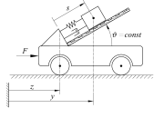
Figure 3: Mass-on-car system. The figure is based on [31, 4].

A spring-damper combination couples the sliding mass $m_{2}$ to the car. Invoking Newton’s mechanical laws, the equations of motion can be derived to be

$$\begin{bmatrix}m_{1}+m_{2}&m_{2}\cos(\vartheta)\\ m_{2}\cos(\vartheta)&m_{2}\end{bmatrix}\!\!\begin{pmatrix}\ddot{z}(t)\\ \ddot{s}(t)\end{pmatrix}\!+\!\begin{pmatrix}0\\ ks(t)+ds(t)\end{pmatrix}=\begin{pmatrix}u(t)\\ 0\end{pmatrix},$$ (12a)

where the horizontal position of the car is $$z s$$, and the relative position of the sliding mass on the car is . The horizontal position of the sliding mass is considered as measured output of the system

$$y(t)=z(t)+\cos(\vartheta)s(t).$$ (12b)

For the numerical simulation we choose the following parameters: inclination angle $\vartheta=\pi/4$, $m_{1}=1$, $m_{2}=2$, spring constant $k=1$, and damping $d=1$. System (12) can be written as a first order system (1), and a short calculation yields that for the chosen parameters it satisfies Assumptions 1, 3 and 2, with relative degree $r=2$. As reference signal we choose $y_{\operatorname*{ref}}=0.4\sin(\tfrac{\pi}{2}t)$ for $t\in[0,2]$, which means that the mass $m_{2}$ on the car is transported from position $0$ to $0.4$ and back to $0$, within chosen error boundaries $\pm 0.15$. We start on the reference, i.e., $y(0)=y_{\rm ref}(0)$, $\dot{y}(0)=\dot{y}_{\rm ref}(0)$, and choose the activation threshold $\lambda=0.75$. As input constraint in the OCP (6) we set $u_{\rm max}=20$, and choose $Q=10^{2}\cdot I$, $R=10^{-4}\cdot I$. Further, we added the regularization term $10^{-6}\cdot\left\|\nu\right\|^{2}$ in the cost functional (6a). With these parameters a brief calculation yields $L_{\rm max}\leq 1.4$, $\gamma_{\rm min}=\gamma_{\rm max}=0.25$, and the gain $\beta\geq 26.98$ is sufficient to guarantee success of the tracking task. Choosing the smallest $\beta$ this already gives $\|u_{\rm ZoH+MPC}\|_{\infty}\leq\max\{\beta/\lambda,u_{\rm max}\}\leq 33.97$. Moreover, we obtain the sampling time $\tau\leq 4.5\cdot 10^{-3}$. We compare the controller (11) with the controller [8], which is (11) with $u_{\rm MPC}^{\star}=0$ (and hence $u_{\rm max}=0$ in (10)), as pointed out earlier. Signals corresponding to the controller (11) are labeled as $y_{\rm ZoH+MPC},u_{\rm ZoH+MPC}$ indicating the application of MPC. Signals corresponding to the controller [8] are labeled with $y_{\rm ZoH},u_{\rm ZoH}$. Now, we consider two scenarios.

V-A Fixed prediction horizon

The prediction horizon for MPC is chosen $L=20$. In Figure 4 the output signals are shown.

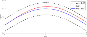
Figure 4: Outputs, reference, and boundaries.

Both controllers achieve the tracking task. However, it can be seen that the controller invoking data-based MPC achieves better tracking performance (the blue line is most of the time very close to the center between the boundaries). In Figure 5 the controls are depicted.

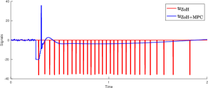
Figure 5: Controls.

As already observed and discussed in [8, Sec. III], the control signal $u_{\rm ZoH}$ consists of separated peaks. This is due to the incorporation of worst-case estimations in the control law. Contrary, the control signal $u_{\rm ZoH+MPC}$ has only one such peak. This comes from the fact, that the data-based MPC produces control signals $u^{\star}_{\rm MPC}$, which are sufficient to keep the error variable $e_{2}$ below the activation threshold $\lambda$, see Figure 7. In particular, the signal $u_{\rm ZoH+MPC}$ is sufficient to achieve the control objective. Figure 6 shows a zoom of the control signals.

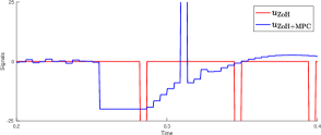
Figure 6: Zoom in controls.

In the beginning, there is random control in order to generate persistently exciting input signal.Then, MPC produces a signal, which is saturated by $u_{\rm max}$; however, it is still sufficient to keep $e_{2}$ below $\lambda$. Shortly after $t=0.3$ the MPC signal is not sufficient and hence the ZoH signal becomes active, resulting in a large control input, which is applied for one sampling interval. Afterwards, MPC again is sufficient to keep $e_{2}$ below $\lambda$. The evolution of the auxiliary error variables $e_{1},e_{2}$ is depicted in Figure 7.

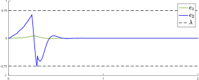
Figure 7: Error variables $e_{1},e_{2}$.

It can be seen, that only at one sampling instance the case $\|e_{2}\|\geq\lambda$ occurs, which then activates the ZoH controller.

V-B Adaptive prediction horizon

We adapt the prediction horizon $L$ in the data-driven MPC, as discussed in Remark III.4. Since with increasing time $t$ more and more system data is available, we update the Hankel matrix (4) in every iteration. Whenever the persistency of excitation order increases, we adapt the prediction horizon $L$. We start with $L=1$ and define an upper limit $L=50$. We compare both controller performances, with fixed prediction horizon $L=20$ (as in the first case), and adaptive horizon. The tracking performance in both settings is comparable, and looks similar to Figure 4. We observed, that adapting the prediction horizon in particular affects the beginning of the simulation, hence, Figure 8 is zoomed in to the beginning. Since we start with $L=1$ in the adaptive setting, the MPC is enabled after few iterations, while for fixed horizon L=20 MPC has to wait until the respective persistency of excitation order is reached. As can be seen from Figure 8 this results in a better control signal for adapted horizon.

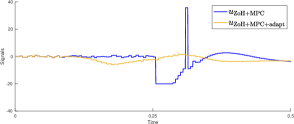
Figure 8: Zoomed in: Controls without and with adapted prediction horizon.

The control signal with adaptive horizon admits two particularities. First, the overall control values are smaller compared to fixed horizon. Second, with adaptive horizon the MPC is able to completely avoid activation of the ZoH component. Hence, no large peaks occur.

VI Conclusion and outlook

We proposed a combined controller, consisting of a sampled-data ZoH feedback component, and a data-driven MPC scheme. While the former ensures safety, i.e., guaranteeing the imposed time-varying output constraints, the latter heavily improves the control performance as illustrated in the presented numerical example. In particular, we showed feasibility of the controller in Proposition IV.1. The presented result defines a starting point towards more sophisticated controller designs, which achieve the control objective “tracking with error guarantees”. Natural extensions of the presented approach will be the consideration of nonlinear systems, uncertain systems, and incorporation of disturbances. Moreover, using the recently introduced notion of collective persistency of excitation [32] would further alleviate the applicability of data-based MPC controllers.

References

- [1] C. P. Bechlioulis and G. A. Rovithakis, “A low-complexity global approximation-free control scheme with prescribed performance for unknown pure feedback systems,” Automatica, vol. 50, no. 4, pp. 1217–1226, 2014.
- [2] I. S. Dimanidis, C. P. Bechlioulis, and G. A. Rovithakis, “Output feedback approximation-free prescribed performance tracking control for uncertain mimo nonlinear systems,” IEEE Transactions on Automatic Control, vol. 65, no. 12, pp. 5058–5069, 2020.
- [3] A. Ilchmann, E. P. Ryan, and C. J. Sangwin, “Tracking with prescribed transient behaviour,” ESAIM: Control, Optimisation and Calculus of Variations, vol. 7, pp. 471–493, 2002.
- [4] T. Berger, A. Ilchmann, and E. P. Ryan, “Funnel control of nonlinear systems,” Mathematics of Control, Signals, and Systems, vol. 33, no. 1, pp. 151–194, 2021.
- [5] D. F. Delchamps, “Stabilizing a linear system with quantized state feedback,” IEEE transactions on automatic control, vol. 35, no. 8, pp. 916–924, 1990.
- [6] R. W. Brockett and D. Liberzon, “Quantized feedback stabilization of linear systems,” IEEE transactions on Automatic Control, vol. 45, no. 7, pp. 1279–1289, 2000.
- [7] X.-H. Chang, R. Huang, H. Wang, and L. Liu, “Robust design strategy of quantized feedback control,” IEEE Transactions on Circuits and Systems II: Express Briefs, vol. 67, no. 4, pp. 730–734, 2019.
- [8] L. Lanza, D. Dennstädt, K. Worthmann, P. Schmitz, G. D. Şen, S. Trenn, and M. Schaller, “Control and safe continual learning of output-constrained nonlinear systems,” arXiv, 2023, submitted, preprint available arXiv:2303.00523.
- [9] J. C. Willems, P. Rapisarda, I. Markovsky, and B. L. M. De Moor, “A note on persistency of excitation,” Systems & Control Letters, vol. 54, no. 4, pp. 325–329, 2005.
- [10] H. Yang and S. Li, “A data-driven predictive controller design based on reduced hankel matrix,” in 2015 10th Asian Control Conference (ASCC). IEEE, 2015, pp. 1–7.
- [11] J. Coulson, J. Lygeros, and F. Dörfler, “Data-enabled predictive control: In the shallows of the DeePC,” in Proc. 2019 18th European Control Conference (ECC). IEEE, 2019, pp. 307–312.
- [12] J. Berberich, J. Köhler, M. A. Müller, and F. Allgöwer, “Data-driven model predictive control with stability and robustness guarantees,” IEEE Transactions on Automatic Control, vol. 66, no. 4, pp. 1702–1717, 2020.
- [13] P. Schmitz, T. Faulwasser, and K. Worthmann, “Willems’ fundamental lemma for linear descriptor systems and its use for data-driven output-feedback MPC,” IEEE Control Systems Letters, vol. 6, pp. 2443–2448, 2022.
- [14] T. Faulwasser, R. Ou, G. Pan, P. Schmitz, and K. Worthmann, “Behavioral theory for stochastic systems? A data-driven journey from Willems to Wiener and back again,” Annual Reviews in Control, 2023.
- [15] G. Pan, R. Ou, and T. Faulwasser, “Towards data-driven stochastic predictive control,” International Journal of Robust and Nonlinear Control, 2022, submitted, arXiv:2212.10663.
- [16] V. G. Lopez and M. A. Müller, “On a continuous-time version of willems’ lemma,” in 2022 IEEE 61st Conference on Decision and Control (CDC), 2022, pp. 2759–2764.
- [17] P. Rapisarda, H. J. van Waarde, and M. K. Camlibel, “A “fundamental lemma” for continuous-time systems, with applications to data-driven simulation,” Available at SSRN 4370211, 2023.
- [18] J. Berberich, J. Köhler, M. A. Müller, and F. Allgöwer, “Linear tracking MPC for nonlinear systems—part II: The data-driven case,” IEEE Transactions on Automatic Control, vol. 67, no. 9, pp. 4406–4421, 2022.
- [19] M. Alsalti, V. G. Berberich, J.and Lopez, F. Allgöwer, and M. A. Müller, “Data-based system analysis and control of flat nonlinear systems,” in Proc. 2021 60th IEEE Conference on Decision and Control (CDC), 2021, pp. 1484–1489.
- [20] I. Markovsky, “Data-driven simulation of nonlinear systems via linear time-invariant embedding,” Vrije Universiteit Brussel, Tech. Rep, 2021.
- [21] I. Markovsky and F. Dörfler, “Behavioral systems theory in data-driven analysis, signal processing, and control,” Annual Reviews in Control, vol. 52, pp. 42–64, 2021.
- [22] F. Albalawi, A. Alanqar, H. Durand, and P. D. Christofides, “Simultaneous control of safety constraint sets and process economics using economic model predictive control,” in 2016 American Control Conference (ACC). IEEE, 2016, pp. 5062–5067.
- [23] Z. Wu, F. Albalawi, Z. Zhang, J. Zhang, H. Durand, and P. D. Christofides, “Control lyapunov-barrier function-based model predictive control of nonlinear systems,” Automatica, vol. 109, p. 108508, 2019.
- [24] J. Pannek and K. Worthmann, “Reducing the prediction horizon in NMPC: An algorithm based approach,” IFAC Proceedings Volumes, vol. 44, no. 1, pp. 7969–7974, 2011.
- [25] P. Giselsson and A. Rantzer, “On feasibility, stability and performance in distributed model predictive control,” IEEE Transactions on Automatic Control, vol. 59, no. 4, pp. 1031–1036, 2013.
- [26] J. Pannek and K. Worthmann, “Stability and performance guarantees for model predictive control algorithms without terminal constraints,” ZAMM-Journal of Applied Mathematics and Mechanics/Zeitschrift für Angewandte Mathematik und Mechanik, vol. 94, no. 4, pp. 317–330, 2014.
- [27] K. Worthmann, M. W. Mehrez, G. K. Mann, R. G. Gosine, and J. Pannek, “Interaction of open and closed loop control in MPC,” Automatica, vol. 82, pp. 243–250, 2017.
- [28] A. J. Krener, “Adaptive horizon model predictive control,” IFAC-PapersOnLine, vol. 51, no. 13, pp. 31–36, 2018.
- [29] A. Isidori, Nonlinear control systems. Springer, 1995.
- [30] T. Berger, H. H. Lê, and T. Reis, “Funnel control for nonlinear systems with known strict relative degree,” Automatica, vol. 87, pp. 345–357, 2018.
- [31] R. Seifried and W. Blajer, “Analysis of servo-constraint problems for underactuated multibody systems,” Mechanical Sciences, vol. 4, no. 1, pp. 113–129, 2013.
- [32] H. J. van Waarde, C. De Persis, M. K. Camlibel, and P. Tesi, “Willems’ fundamental lemma for state-space systems and its extension to multiple datasets,” IEEE Control Systems Letters, vol. 4, no. 3, pp. 602–607, 2020.