VASP2KP: $k\cdot p$ models and Landé $g$-factors from ab initio calculations

Abstract

The $k\cdot p$ method is significant in condensed matter physics for the compact and analytical Hamiltonian. In the presence of magnetic field, it is described by the effective Zeeman’s coupling Hamiltonian with Landé $g$-factors. Here, we develop an open-source package VASP2KP (including two parts: vasp2mat and mat2kp) to compute $k\cdot p$ parameters and Landé $g$-factors directly from the wavefunctions provided by the density functional theory (DFT) as implemented in Vienna ab initio Simulation Package (VASP). First, we develop a VASP patch vasp2mat to compute matrix representations of the generalized momentum operator $\hat{{\bf\it\pi}}=\hat{{\bf\it p}}+\frac{1}{2mc^{2}}\left(\hat{{{\bf\it s}}}\times\nabla V({{\bf\it r}})\right)$, spin operator $\hat{{\bf\it s}}$, time reversal operator $\hat{T}$ and crystalline symmetry operators $\hat{R}$ on the DFT wavefunctions. Second, we develop a python code mat2kp to obtain the unitary transformation $U$ that rotates the degenerate DFT basis towards the standard basis, and then automatically compute the $k\cdot p$ parameters and $g$-factors. The theory and the methodology behind VASP2KP are described in detail. The matrix elements of the operators are derived comprehensively and computed correctly within the projector augmented wave method. We apply this package to some materials, e.g. Bi₂Se₃, Na₃Bi, Te, InAs and 1H-TMD monolayers. The obtained effective model’s dispersions are in good agreement with the DFT data around the specific wave vector, and the $g$-factors are consistent with experimental data. The VASP2KP package is available at https://github.com/zjwang11/VASP2KP.

I Introduction

Electronic band structures hold immense importance in the field of condensed matter physics and materials science, providing crucial insights into the behavior of electrons within crystalline materials. They reveals information about distributions of energy levels, energy gaps, and density of states, which are essential for determining material electrical conductivities, optical properties, thermal behavior, and so on. In this background, the density functional theory (DFT) Hohenberg and Kohn (1964); Kohn and Sham (1965) was developed, which gave birth to many first-principles calculation softwares or codes based on them, including VASP Kresse and Furthmüller (1996, 1996), Quantum Espresso Giannozzi et al. (2009, 2017), CASTEP Clark et al. (2005), ABINIT Gonze et al. (2020); Romero et al. (2020), and so on Soler et al. (2002); García et al. (2020); Blaha et al. (2020); Hourahine et al. (2020).

However, DFT bands are quite complex, which contain quite a large number of energy bands that hardly affect the desired physical properties thus making the physical pictures difficult to understand. In order to construct a model that only involves a few bands with a greater impact on the physical properties of materials, the $k\cdot p$ method is proposed, which is used to construct an effective model to describe the quasiparticles near the specific wave vector in the reciprocal space Luque et al. (2015). The $k\cdot p$ models constructed through the theory of invariants are analytical and only contain a few important bands, thus making the physical pictures quite clear. There are some arbitrary parameters in $k\cdot p$ models, which could be determined by fitting to the corresponding experimental data or the DFT calculation data such as band structures. The $k\cdot p$ method has been successfully applied to many condensed-matter systems, including metals Gresch et al. (2017); Luttinger and Kohn (1955), semiconductors Marquardt et al. (2015); Kane (1957), topological insulators and superconductors Zhang and Zhang (2013); Zhang et al. (2009); Fu (2009); Xu et al. (2011), spin-lasers Faria Junior et al. (2015); Holub and Jonker (2011), nanostructured solids Marquardt (2021), two-dimensional van der Waals materials Faria Junior et al. (2019); Kormányos et al. (2015) and so on Deilmann et al. (2020); Faria Junior and Sipahi (2012); Xuan and Quek (2020); Climente et al. (2016).

When a magnetic field is applied to a condensed matter system, we can use effective Zeeman’s coupling Hamiltonian to describe the effects of the magnetic field. Effective Zeeman’s coupling determines the split of Kramers states under magnetic field, leading to outcomes like the Pauli paramagnetism of the metals and the van Vleck paramagnetism of insulators. The important parameters in Zeeman’s coupling are Landé $g$-factors. Landé $g$-factors of materials have been widely studied in quantum wires Lucignano et al. (2007); Zamani et al. (2017); León-González et al. (2023); Zamani and Rezaei (2018), quantum dots Pryor and Flatté (2006); Gharaati (2017), semiconductors nanostructures Kotlyar et al. (2001); Kiselev et al. (1998); Winkler et al. (2017); Toloza Sandoval et al. (2012); Alegre et al. (2006), topological materials Wang et al. (2015); Liu et al. (2021) and so on Xin and Reid (2002); Semenov et al. (2016); Fischer and Jönsson (2001). Moreover, the theory of invariants can also be used to construct Zeeman’s coupling Hamiltonian conveniently. However, there is no available code to compute Landé $g$-factors and $k\cdot p$ parameters directly from DFT wavefunctions.

First of all, Gao et al. developed the program IRVSP to determine the irreducible representations (irreps) of bands at any ${\bf\it k}$-point in VASP calculations Gao et al. (2021). Then, Jiang et al.  developed the python package kdotp-generator to generate the $k\cdot p$ effective Hamiltonian for the given irreps automatically Jiang et al. (2021). Furthermore, Song et al. derived effective Zeeman’s coupling and $g$-factors in DFT calculations Song et al. (2021). Thus, it is straightforward for us to generate the VASP2KP code to construct the effective models and to compute the model parameters from VASP wavefunctions directly. Although many similar codes are developed subsequently for Quantum Espresso, such as IR2PW Zhang et al. (2023a), IrRep Iraola et al. (2022), and DFT2kp Cassiano et al. (2023), their functions do not go beyond the above mentioned codes. The DFT2kp can not generate the Zeeman’s coupling Hamiltonians. Additionally, the matrix elements of symmetry operators are not obtained properly, because the projector augmented wave (PAW) corrections are neglected in DFT2kp.

In this work, we have developed an open-source package VASP2KP, which can generate the effective $k\cdot p$ model and Zeeman’s coupling, and obtain the values of the $k\cdot p$ parameters and $g$-factors. This package contains two parts: a VASP patch vasp2mat and a post-processing python code mat2kp. First, we use vasp2mat to generate matrix representations for generalized momentum $\hat{{\bf\it\pi}}=\hat{{\bf\it p}}+\frac{1}{2mc^{2}}(\hat{{\bf\it s}}\times\nabla V({\bf\it r}))$, spin $\hat{{\bf\it s}}$, time reversal $\hat{T}$, and crystalline symmetry operators $\hat{R}$ in DFT calculations. The matrix elements of the space group operators are derived in detail and computed correctly in the PAW wavefunctions. Second, mat2kp can obtain the unitary transformation $U$ from the degenerate wavefunctions to the $k\cdot p$ standard basis, and then compute these parameters automatically. The obtained effective masses and $g$-factors are important and comparable with experimental observations.

The paper is organized as the following. In Sec. II, the theoretical foundations behind VASP2KP are introduced. In Sec. III the main algorithm steps are described in detail. The results obtained by VASP2KP are shown and analysed for some typical materials in Sec. IV, and we have some discussions in Sec. V.

II Theory and methodology

In this section, we first introduce the $k\cdot p$ method in Sec. II.1. The method to obtain Zeeman’s coupling is presented in Sec. II.2. Then the theory of invariants is reviewed and the invariant $k\cdot p$ Hamiltonian as well as Zeeman’s coupling are obtained in Sec. II.3. In Sec. II.4, we propose a general routine to get the unitary transformation that change degenerate DFT basis to the $k\cdot p$ standard basis. Last, the method to calculate $k\cdot p$ parameters and $g$-factors is introduced in Sec. II.5.

II.1 $k\cdot p$ effective Hamiltonian

When we only care about wave vector ${{\bf\it K}}$ around a specific wave vector ${{\bf\it k}}_{0}$ in the Brillouin zone, it can be well described by using the $k\cdot p$ effective model. Suppose that $\psi_{n{{\bf\it K}}}({{\bf\it r}})$ is the wavefunction of $n$-th band which satisfies the Schrödinger equation with spin-orbit coupling (SOC), i.e., $\hat{H}_{B}\psi_{n{{\bf\it K}}}({{\bf\it r}})=\epsilon_{n}({{\bf\it K}})\psi_{n{{\bf\it K}}}({{\bf\it r}})$, where

$$\hat{H}_{B}=\frac{\hat{p}^{2}}{2m}+V({{\bf\it r}})+\frac{1}{2m^{2}c^{2}}\left(\hat{{{\bf\it s}}}\times\nabla V({{\bf\it r}})\right)\cdot\hat{{{\bf\it p}}}$$ (1)

is the Bloch Hamiltonian operator with SOC, and $\hat{{\bf\it p}}$ is the momentum operator, $V({{\bf\it r}})$ is the potential in crystal, $\hat{{{\bf\it s}}}$ is the spin momentum operator, $m$ is the electron mass, and $c$ is the light speed in vacuum. To expand the Hamiltonian at ${\bf\it k}_{0}$, introducing a transformation $\phi_{n{{\bf\it k}}}({{\bf\it r}})=\psi_{n{{\bf\it K}}}({{\bf\it r}})e^{-i{\bf\it k}\cdot{\bf\it r}}$, where ${{\bf\it k}}={{\bf\it K}}-{{\bf\it k}}_{0}$ is the deviation from ${{\bf\it k}}_{0}$, the Schrödinger equation which $\phi_{{\bf\it k}}({{\bf\it r}})$ obeys is

$$\left(\hat{H}_{B}+\frac{\hbar^{2}k^{2}}{2m}+\hat{H}^{\prime}({{\bf\it k}})\right)\phi_{n{{\bf\it k}}}({{\bf\it r}})=\epsilon_{n}({{\bf\it K}})\phi_{n{{\bf\it k}}}({{\bf\it r}})$$ (2)

where $\hat{H}^{\prime}({{\bf\it k}})=\frac{\hbar}{m}{{\bf\it k}}\cdot{{\bf\it\pi}}$ is the first-order term, and $\hat{{\bf\it\pi}}=\hat{{\bf\it p}}+\frac{1}{2mc^{2}}\left(\hat{{{\bf\it s}}}\times\nabla V({{\bf\it r}})\right)$ is the generalized momentum operator with SOC. We can take $\hat{H}^{kp}=\hat{H}_{B}+\frac{\hbar^{2}k^{2}}{2m}+\hat{H}^{\prime}({{\bf\it k}})$ as the equivalent Hamiltonian of $\hat{H}_{B}$ since the eigenvalues of them are all equal.

Suppose that we have got the eigenenergies $\{\epsilon_{n}({{\bf\it k}}_{0})\}$ and the eigenstates $\{\ket{n({{\bf\it k}}_{0})}\}$ of $\hat{H}_{B}$. Then we can obtain the generalized momentum elements by ${{\bf\it\pi}}_{mn}=\matrixelement{m({{\bf\it k}}_{0})}{\hat{{\bf\it\pi}}}{n({{\bf\it k}}_{0})}$. Thus the matrix elements of $\hat{H}^{kp}$ can be obtained by

$$H^{\text{kp-all}}_{mn}({{\bf\it k}})=\left(\epsilon_{n}({{\bf\it k}}_{0})+\frac{\hbar^{2}k^{2}}{2m}\right)\delta_{mn}+\frac{\hbar}{m}{{\bf\it\pi}}_{mn}\cdot{{\bf\it k}}$$ (3)

Usually, we aimed at several low-energy bands (the set of which is denoted as $\mathcal{A}$). The set of other bands is denoted as $\mathcal{B}$. Then we can fold down the $H^{\text{kp-all}}_{mn}({{\bf\it k}})$ Hamiltonian into a subspace $\mathcal{A}$ via Löwdin partitioning. After two-order Löwdin partitioning, the effective $k\cdot p$ Hamiltonian is transformed as (see Appendix A for details)

$$H^{kp}_{\alpha\beta}({{\bf\it k}})= \left(\epsilon_{\alpha}({{\bf\it k}}_{0})+\frac{\hbar^{2}k^{2}}{2m}\right)\delta_{\alpha\beta}+\frac{\hbar}{m}{{\bf\it\pi}}_{\alpha\beta}\cdot{{\bf\it k}}$$ (4)

$$+\frac{\hbar^{2}}{2m^{2}}\sum_{l\in\mathcal{B}}\sum_{ij}\pi^{i}_{\alpha l}\pi^{j}_{l\beta}k^{i}k^{j}$$

$$\times\left(\frac{1}{\epsilon_{\alpha}({{\bf\it k}}_{0})-\epsilon_{l}({{\bf\it k}}_{0})}+\frac{1}{\epsilon_{\beta}({{\bf\it k}}_{0})-\epsilon_{l}({{\bf\it k}}_{0})}\right)$$

with $i,j\in\{x,y,z\}$. Hereafter we use $\alpha,\beta\in\mathcal{A}$, $l\in\mathcal{B}$ and $m,n\in\mathcal{A}\cup\mathcal{B}$. Moreover, the $k\cdot p$ Hamiltonian of the third order can be constructed similarly in Appendix A.

II.2 Zeeman’s coupling

When a magnetic field is applied to the system, the momenta $\hbar k^{i}$ should be replaced by $(-i\hbar\partial^{i}+eA^{i})$ according to Peierls substitution, where ${{\bf\it A}}$ is the vector potential and $e$ (positively valued) is the elementary charge. Therefore, $\hbar^{2}k^{i}k^{j}$ in the summation will be replaced by the sum of the gauge dependent term $\frac{1}{2}\left\{-i\hbar\partial^{i}+eA^{i},-i\hbar\partial^{j}+eA^{j}\right\}$ and gauge independent term $\frac{1}{2}\left[-i\hbar\partial^{i}+eA^{i},-i\hbar\partial^{j}+eA^{j}\right]=-\frac{i\hbar e}{2}\sum_{k}\epsilon^{ijk}B_{k}$, where ${{\bf\it B}}$ is the magnetic induction intensity. In this case, the total Hamiltonian can be written by the summation of the $k\cdot p$ effective Hamiltonian $H^{kp}_{\alpha\beta}$ and Zeeman’s coupling $H^{Z}_{\alpha\beta}$, which are gauge dependent and gauge invariant, respectively. The $k\cdot p$ effective Hamiltonian $H^{kp}_{\alpha\beta}$ can be expressed as

$$\begin{aligned} H^{kp}_{\alpha\beta}=&\epsilon_{\alpha}({{\bf\it k}}_{0})\delta_{\alpha\beta}+\frac{\hbar}{m}{{\bf\it\pi}}_{\alpha\beta}\cdot\left(-i\nabla+\frac{e}{\hbar}{{\bf\it A}}\right)\\ &+\sum_{ij}M_{\alpha\beta}^{ij}\left(-i\partial^{i}+\frac{e}{\hbar}A^{i}\right)\left(-i\partial^{j}+\frac{e}{\hbar}A^{j}\right)\end{aligned},$$ (5)

where

$$\begin{aligned} M_{\alpha\beta}^{ij}=&\frac{\hbar^{2}}{2m}\delta_{\alpha\beta}\delta_{ij}+\frac{\hbar^{2}}{4m^{2}}\sum_{l\in\mathcal{B}}\left(\pi^{i}_{\alpha l}\pi^{j}_{l\beta}+\pi^{j}_{\alpha l}\pi^{i}_{l\beta}\right)\\ &\times\left(\frac{1}{\epsilon_{\alpha}({{\bf\it k}}_{0})-\epsilon_{l}({{\bf\it k}}_{0})}+\frac{1}{\epsilon_{\beta}({{\bf\it k}}_{0})-\epsilon_{l}({{\bf\it k}}_{0})}\right)\end{aligned}.$$ (6)

Zeeman’s coupling term can be expressed by

$$H^{Z}_{\alpha\beta}=\frac{\mu_{B}}{\hbar}\left({{\bf\it L}}_{\alpha\beta}+2{{\bf\it s}}_{\alpha\beta}\right)\cdot{{\bf\it B}},$$ (7)

where

$$L_{\alpha\beta}^{k}= -\frac{i\hbar}{2m}\sum_{l\in\mathcal{B}}\sum_{ij}\epsilon^{ijk}\pi^{i}_{\alpha l}\pi^{j}_{l\beta}$$ (8)

$$\times\left(\frac{1}{\epsilon_{\alpha}({{\bf\it k}}_{0})-\epsilon_{l}({{\bf\it k}}_{0})}+\frac{1}{\epsilon_{\beta}({{\bf\it k}}_{0})-\epsilon_{l}({{\bf\it k}}_{0})}\right)$$

can be considered as the orbital contribution, ${{\bf\it s}}_{\alpha\beta}=\matrixelement{\alpha({{\bf\it k}}_{0})}{\hat{{{\bf\it s}}}}{\beta({{\bf\it k}}_{0})}$ are the spin elements, and $\mu_{B}$ is the Bohr magneton. The detailed derivation is shown in Appendix B.

II.3 Theory of invariants

Suppose that the little group at ${{\bf\it k}}_{0}$ is $L$, and $D(R)$ is a representation (rep) for $\forall R\in L$, whose dimension is $N$. There are a total of $N^{2}$ independent Hermitian matrices ${{\bf\it X}}={X_{i}\ (i=1,2,\cdots,N^{2})}$ in $N$ dimensions that constitute an $N$-dimensional matrix space. It is simple to get a new rep $D^{(X)}$ by

$$D(R)X_{n}D(R)^{-1}=\sum_{m}X_{m}D^{(X)}_{mn}(R)$$ (9)

for $\forall R\in L$. Also, we can construct polynomial space of order $p\in\mathbb{N}$, whose basis can be chosen as ${{\bf\it g}}({{\bf\it k}})=\{k_{x}^{i}k_{y}^{j}k_{z}^{l}|i+j+l\leq p,i,j,l\in\mathbb{N}\}$. It is simple to get a new rep $D^{(g)}$ by

$$\hat{R}g_{n}({\bf\it k})=g_{n}(R^{-1}{{\bf\it k}})=\sum_{m}g_{m}({{\bf\it k}})D^{(g)}_{mn}(R).$$ (10)

Spatial inversion $\hat{P}$ and time reversal $\hat{T}$ may also be the elements of the little group $L$, which transform the wave vector as ${\bf\it k}\xrightarrow{\hat{P}}-{\bf\it k}$ and ${\bf\it k}\xrightarrow{\hat{T}}-{\bf\it k}$, respectively.

Decomposing $D^{(X)}$ and $D^{(g)}$ into irreps, we have

$$D^{(X)}(R)\simeq\bigoplus_{\lambda}a_{\lambda}D^{\lambda}(R)$$ (11)

$$D^{(g)}(R)\simeq\bigoplus_{\lambda}b_{\lambda}D^{\lambda}(R)$$ (12)

where $D^{\lambda}$ represents irreps and $a_{\lambda}$ or $b_{\lambda}$ denotes the multiplicities of $D^{\lambda}$. Note that the irreps decomposed from the $D^{(X)}$ and $D^{(g)}$ are not exactly the same. It is simple to get the matrix basis $X^{\lambda,\mu}$ and polynomial basis ${\bf\it g}^{\lambda,\nu}({\bf\it k})$ of $D^{\lambda}$-irrep. An irrep may correspond to more than one sets of matrix basis or polynomial basis, thus enabling us to add an indicator $\mu/\nu$ to distinguish them. After obtaining matrix basis and polynomial basis, the $k\cdot p$ Hamiltonian can be written as

$$H^{kp}({{\bf\it k}})=\sum_{\lambda}\sum_{\mu=1}^{a_{\lambda}}\sum_{\nu=1}^{b_{\lambda}}c_{\lambda\mu\nu}{\bf\it X}^{\lambda,\mu}\cdot{\bf\it g}^{*\lambda,\nu}({{\bf\it k}}),$$ (13)

where $c_{\lambda\mu\nu}$ are undetermined $k\cdot p$ parameters, which must be real Jiang et al. (2021). It can be proved that the $p$-th order $k\cdot p$ Hamiltonian expressed by Eq. (13) satisfies the relation

$$H^{kp}(\hat{R}{{\bf\it k}})=D(R)H^{kp}({{\bf\it k}})D(R)^{-1}$$ (14)

for $\forall R\in L$ Jiang et al. (2021).

Moreover, in the presence of magnetic field, Zeeman’s coupling can also be constructed in the same way. Unlike the wave vector ${\bf\it k}$, the magnetic field ${\bf\it B}$ is a pseudovector, thus making it satisfy the relation ${\bf\it B}\xrightarrow{\hat{P}}{\bf\it B}$ and ${\bf\it B}\xrightarrow{\hat{T}}-{\bf\it B}$ under spatial inversion and time reversal, respectively. Effective Zeeman’s coupling satisfies the relation

$$H^{Z}(\hat{R}{\bf\it B})=D(R)H^{Z}({\bf\it B})D(R)^{-1}$$ (15)

By the way, given the matrix representations of the generators of the little group $L$, the python package kdotp-generator constructs the standard $k\cdot p$ Hamiltonian or Zeeman’s coupling with undetermined $k\cdot p$ parameters as Eq. (13). The standard matrices $D^{\text{std}}(R)$ are given on the Bilbao Crystalline Server (BCS) for the assigned irreps by IRVSP .

II.4 Unitary transformation

In DFT calculations, when the irrep is $n$-fold ($n\geq 2$) and the eigenstates are degenerate, there is $U(n)$ ambiguity in the DFT eigenstates. In this section, we propose a general routine to get the unitary transformation that changes degenerate DFT wavefunctions to the $k\cdot p$ standard basis. We can obtain the eigenenergies $\{\epsilon_{n}({{\bf\it k}}_{0})\}$ and eigenstates $\{\ket{n({{\bf\it k}}_{0})}\}$ in VASP. The matrix representation of $\hat{R}$ under the VASP basis set would be calculated by mat2kp, which is denoted as $D^{\text{num}}(R)$.

However, $D^{\text{num}}(R)$ is usually not in the standard form; they are related by a unitary transformation, i.e.,

$$D^{\text{std}}(R)=U^{\dagger}D^{\text{num}}(R)U$$ (16)

for $\forall R\in L$, where $U$ is a unitary matrix. To find $U$, it is obvious that only the generators of the ${\bf\it k}_{0}$-little group $L$ should be taken into account. They are space group operators $\{R_{t}|{\bf\it v}_{t}\}$, consisting of rotational part and translational part. The translational part is usually expressed by a phase factor. The Eq. (16) can be rewritten as

$$D^{\text{num}}(R)U-UD^{\text{std}}(R)={\bf\it 0}$$ (17)

where ${\bf\it 0}$ is a zero matrix. The real part and the imaginary part of each elements of $U$ are independent variables, which are denoted as $U_{r11},U_{r12},\cdots U_{rnn}$ and $U_{i11},U_{i12},\cdots U_{inn}$, respectively. From Eq. (17), it is clear to find that all these variables satisfy a linear equation set. Using a column vector ${{\bf\it u}}=(U_{r11},U_{r12},\cdots,U_{rnn},U_{i11},U_{i12},\cdots,U_{inn})^{T}$, the Eq. (17) can be rewritten as

$$Q{{\bf\it u}}={\bf\it 0}$$ (18)

where $Q$ is a real coefficient matrix defined by Eq. (17). The details are shown in Appendix C.

Therefore, all vectors in the null space of the matrix $Q$ is the solution to Eq. (16). Perform singular value decomposition on matrix $Q$, we can obtain $Q=V_{1}\Sigma V_{2}^{T}$ thus $QV_{2}=V_{1}\Sigma$, where $V_{1}$ and $V_{2}$ are orthogonal matrices and $\Sigma$ is a diagonal matrix. It can be proved that the column vectors in $V_{1}$ correspond to the singular value 0 form the basis of the null space of the matrix $Q$, which are denoted as $\{{{\bf\it u}_{1}},{{\bf\it u}_{2}},\cdots,{{\bf\it u}_{m}}\}$. After reshaping these vectors, the basis of the solution space of $U$ of Eq. (16) are denoted as $\{U_{1},U_{2},\cdots,U_{n}\}$. Any solution can be written as

$$U=\sum_{\alpha=1}^{m}\lambda_{\alpha}U_{\alpha}$$ (19)

where $\lambda_{\alpha}$ must be real.

Thus, one has to get one set of the parameters $\{\lambda_{\alpha}\}$ to satisfy $U^{\dagger}U=\mathbb{I}$, where $\mathbb{I}$ is an identity matrix. However, this relation is nonlinear, thus making it hard to solve by treating it as an equation directly. In mat2kp, the unitary $U$ is obtained via the sequential least squares programming to find optimal parameter set $\{\lambda_{\alpha}\}$, which can minimize the error $\varepsilon=\sum_{ij}\left|(U^{\dagger}U-\mathbb{I})_{ij}\right|$.

II.5 Calculations of parameters

Applying Eqs. (4-8) in DFT calculations, one can get the numerical Hamiltonian $H^{\text{num}}$, one have to solve the equation $H^{\text{std}}=U^{-1}H^{\text{num}}U$ to get all the parameters in $H^{\text{std}}$. By the way, from Eq. (13), it is easy to find that the equations are all linear equations. However, there are more equations than parameters. The coefficients of each linear equation are not accurate because of numerical errors generated from VASP calculations, making it impossible to solve by the traditional Gaussian elimination method. We can write all equations in a matrix form

$$A\bm{x}=\bm{b},$$ (20)

where $A$ is a constant matrix, and $\bm{x}$ is the column vector comprised of all undetermined real parameters. To eliminate the constraint of the real $\bm{x}$, suppose that $A=A_{r}+iA_{i}$ and $\bm{b}=\bm{b}_{r}+i\bm{b}_{i}$, where the subscript $r$ represents the real part and the subscript $i$ represents the imaginary part. Then Eq. (20) can be transformed as

$$\left(\begin{aligned} A_{r}\\ A_{i}\end{aligned}\right)\bm{x}=\left(\begin{aligned} \bm{b}_{r}\\ \bm{b}_{i}\end{aligned}\right).$$ (21)

In this case, all the matrices become real (the real constraint is automatically satisfied). Therefore, the linear least square method can be used to calculate the parameters and to give the error as well.

III Capability of VASP2KP

The VASP2KP package contains two parts: the VASP patch vasp2mat and the post-processing python code mat2kp. The workflow is presented in Fig. 1. The methodology of obtaining the matrix elements of the generalized momentum, spin, time reversal and crystalline rotational operators in VASP is introduced in Sec. III.1. The main algorithm steps of VASP2KP are described in Sec. III.2. Lastly, main steps to construct $k\cdot p$ models and Zeeman’s coupling via VASP2KP are shown in Sec. III.3.

III.1 vasp2mat: to compute matrix elements from DFT wavefunctions

The matrix elements of $\hat{{\bf\it\pi}}$, $\hat{{\bf\it s}}$, $\hat{T}$ and $\hat{R}$ are required in constructing the $k\cdot p$ Hamiltonian and Zeeman’s coupling under the DFT wavefunctions as shown in Sec. II.1. The computation method of $\hat{{\bf\it\pi}}$ matrix elements was first introduced in Ref. Song et al. (2021). Here we generalize it to nonlocal operators. In VASP, the PAW potential is used, which is a combination and generalization of the linear augmented plane wave method. Therefore, we derive these matrix elements under the PAW wavefunctions, which are implemented in vasp2mat to compute the matrix elements.

The relation of all electron wavefunction ($\ket{n({\bf\it k}_{0})}$) and pseudo wavefunction ($\ket{\widetilde{n}({\bf\it k}_{0})}$) in PAW is

$$\ket{n({\bf\it k}_{0})}=\mathcal{T}\ket{\widetilde{n}({\bf\it k}_{0})},$$ (22)

where the linear transformation $\mathcal{T}$ can be expressed as Blöchl (1994); Blöchl et al. (2003)

$$\mathcal{T}=1+\sum_{a\mu\zeta}\left(\ket{\phi^{a}_{\mu}\zeta}-\ket{\widetilde{\phi}^{a}_{\mu}\zeta}\right)\bra{\widetilde{p}^{a}_{\mu}\zeta}.$$ (23)

The $\ket{\phi^{a}_{\mu}\zeta}$ is the direct product of the real space all electron partial wavefunction $\phi^{a}_{\mu}({\bf\it r})$ at the $a$-th atom with a spinor wavefunction $\ket{\zeta}(\zeta=\uparrow\text{or}\downarrow)$, $\ket{\widetilde{\phi}^{a}_{\mu}\zeta}$ is the direct product of the real space pseudo partial wavefunction $\widetilde{\phi}^{a}_{\mu}({\bf\it r})$ with a spinor wavefunction $\ket{\zeta}$, and $\ket{\widetilde{p}^{a}_{\mu}\zeta}$ is a projector wavefunction comprised of the direct product of a real space projector wavefunction $\widetilde{p}^{a}_{\mu}({{\bf\it r}})$ and a spinor wavefunction $\ket{\zeta}$. Here, $\phi^{a}_{\mu}({\bf\it r})$’s are obtained by all-electron calculation for the reference atom. The pseudo partial wavefunctions $\widetilde{\phi}^{a}_{\mu}({\bf\it r})$ are identical to $\phi^{a}_{\mu}({\bf\it r})$ outside the augmentation sphere of the corresponding atom and are much softer than $\phi^{a}_{\mu}({\bf\it r})$ inside the augmentation sphere; $\widetilde{\phi}^{a}_{\mu}({\bf\it r})$’s provide a complete basis for the pseudo wavefunction $\ket{\widetilde{n}(\bm{k}_{0})}$ inside the augmentation sphere. The projector wavefunctions are defined in such a way, i.e., $\langle\widetilde{p}^{a}_{\mu}|\widetilde{\phi}^{a}_{\mu^{\prime}}\rangle=\delta_{\mu\mu^{\prime}}$, that $\langle\widetilde{p}_{\mu}^{a}\zeta|\widetilde{n}(\bm{k}_{0})\rangle$ gives the expanding coefficients of $|\widetilde{n}(\bm{k}_{0})\rangle$ on $\widetilde{\phi}^{a}_{\mu}({\bf\it r})$. Usually the projector wavefunctions are chosen to be zero outside the core radius. Therefore, outside the augmentation sphere the third and second terms in $\mathcal{T}$ cancel each other exactly, and inside the augmentation sphere the first and third terms cancel each other exactly. $\mathcal{T}$ leaves $|\widetilde{n}(\bm{k}_{0})\rangle$ unchanged outside the augmentation sphere and maps it to the all-electron wavefunction inside the augmentation sphere. Both ${\phi}^{a}_{\mu}({\bf\it r})$ and $\widetilde{\phi}^{a}_{\mu}({\bf\it r})$ are stored as a radial part times an angular part, which can be expressed as

$$\left\{\begin{aligned} \phi^{a}_{\mu}({\bf\it r})=Y^{m_{\mu}}_{l_{\mu}}(\widehat{{\bf\it r}-{{\bf\it\tau}}_{a}})R^{a}_{\mu}(\left|{\bf\it r}-{{\bf\it\tau}}_{a}\right|)\\ \widetilde{\phi}^{a}_{\mu}({\bf\it r})=Y^{m_{\mu}}_{l_{\mu}}(\widehat{{\bf\it r}-{{\bf\it\tau}}_{a}})\widetilde{R}^{a}_{\mu}(\left|{\bf\it r}-{{\bf\it\tau}}_{a}\right|)\end{aligned}\right.$$ (24)

where ${{\bf\it\tau}}_{a}$ is the site of the $a$-th atom, $Y^{m}_{l}$ are sphere harmonics, and $R^{a}_{\mu}$ are real functions. The hatted vectors represent the unit vector along the corresponding directions.

According to Eq. (23), the PAW matrix form of a local operator $\hat{F}$ can be expressed by

$$\begin{aligned} F_{mn}=&\matrixelement{m({\bf\it k}_{0})}{\hat{F}}{n({\bf\it k}_{0})}=\matrixelement{\widetilde{m}({\bf\it k}_{0})}{\mathcal{T}^{\dagger}\hat{F}\mathcal{T}}{\widetilde{n}({\bf\it k}_{0})}\\ =&\matrixelement{\widetilde{m}({\bf\it k}_{0})}{\hat{F}}{\widetilde{n}({\bf\it k}_{0})}\\ &+\sum_{a\mu\nu}\sum_{\zeta\zeta^{\prime}}\innerproduct{\widetilde{m}({\bf\it k}_{0})}{\widetilde{p}^{a}_{\mu}\zeta}F^{a}_{\mu\zeta,\nu\zeta^{\prime}}\innerproduct{\widetilde{p}^{a}_{\nu}\zeta^{\prime}}{\widetilde{n}({\bf\it k}_{0})}\end{aligned},$$ (25)

where $F^{a}_{\mu\zeta,\nu\zeta^{\prime}}$ is the projection matrix of the operator $\hat{F}$ in the $a$-th atom’s augmentation sphere, which is defined as

$$F^{a}_{\mu\zeta,\nu\zeta^{\prime}}=\matrixelement{\phi^{a}_{\mu}\zeta}{\hat{F}}{\phi^{a}_{\nu}\zeta^{\prime}}-\matrixelement{\widetilde{\phi}^{a}_{\mu}\zeta}{\hat{F}}{\widetilde{\phi}^{a}_{\nu}\zeta^{\prime}}.$$ (26)

The first term in $F^{a}_{\mu\zeta,\mu^{\prime}\zeta^{\prime}}$ gives the contribution from the all-electron wavefunction in the augmentation sphere, and the second term cancels the contribution from the pseudo wavefunction in the augmentation sphere that is counted in the first term of Eq. (25).

In PAW, the plane wave is used to span the pseudo wavefunction $\widetilde{\psi}_{n{\bf\it k}_{0}}({\bf\it r},\zeta)=\innerproduct{{\bf\it r},\zeta}{\widetilde{n}({\bf\it k}_{0})}$, which is expressed by

$$\widetilde{\psi}_{n{\bf\it k}_{0}}({\bf\it r},\zeta)=\sum_{{\bf\it G}}c^{n{\bf\it k}_{0}}_{\zeta{\bf\it G}}e^{i({{\bf\it k}_{0}+{\bf\it G}})\cdot{{\bf\it r}}}$$ (27)

where $c^{n{\bf\it k}_{0}}_{\zeta{\bf\it G}}$ are the plane wave coefficients.

The projection coefficients $\innerproduct{\widetilde{p}^{a}_{\mu}\zeta}{\widetilde{n}({\bf\it k}_{0})}$ in the second term of Eq. (25) have already been calculated in VASP. Therefore, to calculate the matrix of the local operator $\hat{F}$, we need to calculate $\matrixelement{\widetilde{m}({\bf\it k}_{0})}{\hat{F}}{\widetilde{n}({\bf\it k}_{0})}$ and $F^{a}_{\mu\zeta,\nu\zeta^{\prime}}$ in Eq. (25).

III.1.1 Generalized momentum matrix

The matrix of the generalized momentum $\hat{{\bf\it\pi}}$ can be expressed by substituting $\hat{{\bf\it\pi}}$ into $\hat{F}$ in Eq. (25) as follows:

$${\bf\it\pi}_{mn}=\matrixelement{\widetilde{m}({\bf\it k}_{0})}{\hat{{\bf\it p}}}{\widetilde{n}({\bf\it k}_{0})}+\frac{1}{2mc^{2}}\matrixelement{\widetilde{m}({\bf\it k}_{0})}{\hat{{\bf\it s}}\times\nabla V}{\widetilde{n}({\bf\it k}_{0})}$$ (28)

$$+ \sum_{a\mu\nu}\sum_{\zeta\zeta^{\prime}}\innerproduct{\widetilde{m}({\bf\it k}_{0})}{\widetilde{p}^{a}_{\mu}\zeta}{\bf\it p}^{a}_{\mu\zeta,\nu\zeta^{\prime}}\innerproduct{\widetilde{p}^{a}_{\nu}\zeta^{\prime}}{\widetilde{n}({\bf\it k}_{0})}$$

$$+ \frac{1}{2mc^{2}}\sum_{a\mu\nu\zeta\zeta^{\prime}}\innerproduct{\widetilde{m}({\bf\it k}_{0})}{\widetilde{p}^{a}_{\mu}\zeta}\matrixelement{\phi^{a}_{\mu}\zeta}{\hat{{\bf\it s}}\times\nabla V}{\phi^{a}_{\nu}\zeta^{\prime}}\innerproduct{\widetilde{p}^{a}_{\nu}\zeta^{\prime}}{\widetilde{n}({\bf\it k}_{0})}$$

$$- \frac{1}{2mc^{2}}\sum_{a\mu\nu\zeta\zeta^{\prime}}\innerproduct{\widetilde{m}({\bf\it k}_{0})}{\widetilde{p}^{a}_{\mu}\zeta}\matrixelement{\widetilde{\phi}^{a}_{\mu}\zeta}{\hat{{\bf\it s}}\times\nabla V}{\widetilde{\phi}^{a}_{\nu}\zeta^{\prime}}\innerproduct{\widetilde{p}^{a}_{\nu}\zeta^{\prime}}{\widetilde{n}({\bf\it k}_{0})}$$

Since the SOC effect is considered only within the augmentation spheres in VASP, where $\ket{\widetilde{n}({\bf\it k}_{0})}=\sum_{a\mu\zeta}\ket{\widetilde{\phi}^{a}_{\mu}\zeta}\innerproduct{\widetilde{p}^{a}_{\mu}\zeta}{\widetilde{n}({\bf\it k}_{0})}$, we can make the second term and the fifth term in Eq. (28) cancel out. Therefore, the generalized momentum matrix can be simplified to

$${\bf\it\pi}_{mn}= \matrixelement{\widetilde{m}({\bf\it k}_{0})}{\hat{{\bf\it p}}}{\widetilde{n}({\bf\it k}_{0})}$$ (29)

$$+\sum_{a\mu\nu}\sum_{\zeta\zeta^{\prime}}\innerproduct{\widetilde{m}({\bf\it k}_{0})}{\widetilde{p}^{a}_{\mu}\zeta}{\bf\it\pi}^{\prime a}_{\mu\zeta,\nu\zeta^{\prime}}\innerproduct{\widetilde{p}^{a}_{\nu}\zeta^{\prime}}{\widetilde{n}({\bf\it k}_{0})}$$

where

$${\bf\it\pi}^{\prime a}_{\mu\zeta,\nu\zeta^{\prime}}= \delta_{\zeta\zeta^{\prime}}\left(\matrixelement{\phi^{a}_{\mu}}{\hat{{{\bf\it p}}}}{\phi^{a}_{\nu}}-\matrixelement{\widetilde{\phi}^{a}_{\mu}}{\hat{{{\bf\it p}}}}{\widetilde{\phi}^{a}_{\nu}}\right)$$ (30)

$$+\frac{\hbar^{2}}{4mc^{2}}{\bf\it\sigma}_{\zeta\zeta^{\prime}}\times\matrixelement{\phi^{a}_{\mu}}{\nabla V}{\phi^{a}_{\nu}}$$

The first term of ${\bf\it\pi}_{mn}$ in Eq. (29) can be calculated by

$$\matrixelement{\widetilde{m}({\bf\it k}_{0})}{\hat{{\bf\it p}}}{\widetilde{n}({\bf\it k}_{0})}=\sum_{{\bf\it G}}\hbar({\bf\it k}_{0}+{\bf\it G})c^{*m{\bf\it k}_{0}}_{\zeta{\bf\it G}}c^{n{\bf\it k}_{0}}_{\zeta{\bf\it G}}$$ (31)

where $\hat{{\bf\it p}}=-i\hbar\nabla$. The integrals in ${\bf\it\pi}^{\prime a}_{\mu\zeta,\nu\zeta^{\prime}}$ can be calculated by separating the radial part and angular part, which are expressed as

$$\left\{\begin{aligned} &\begin{aligned} \matrixelement{\phi^{a}_{\mu}}{\hat{{{\bf\it p}}}}{\phi^{a}_{\nu}}&=-i\hbar\int\mathrm{d}\Omega Y^{m_{\mu}*}_{l_{\mu}}\nabla Y^{m_{\nu}}_{l_{\nu}}\int\mathrm{d}rr^{2}R^{a*}_{\mu}R^{a}_{\nu}\\ &-i\hbar\int\mathrm{d}\Omega Y^{m_{\mu}*}_{l_{\mu}}\frac{{\bf\it r}}{r}Y^{m_{\nu}}_{l_{\nu}}\int\mathrm{d}rr^{2}R^{a*}_{\mu}\partial_{r}R^{a}_{\nu}\end{aligned}\\ &\begin{aligned} \matrixelement{\widetilde{\phi}^{a}_{\mu}}{\hat{{{\bf\it p}}}}{\widetilde{\phi}^{a}_{\nu}}=&-i\hbar\int\mathrm{d}\Omega Y^{m_{\mu}*}_{l_{\mu}}\nabla Y^{m_{\nu}}_{l_{\nu}}\int\mathrm{d}rr^{2}\widetilde{R}^{a*}_{\mu}\widetilde{R}^{a}_{\nu}\\ &-i\hbar\int\mathrm{d}\Omega Y^{m_{\mu}*}_{l_{\mu}}\frac{{\bf\it r}}{r}Y^{m_{\nu}}_{l_{\nu}}\int\mathrm{d}rr^{2}\widetilde{R}^{a*}_{\mu}\partial_{r}\widetilde{R}^{a}_{\nu}\end{aligned}\\ &\matrixelement{\phi^{a}_{\mu}}{\nabla V}{\phi^{a}_{\nu}}\approx\int\mathrm{d}\Omega Y^{m_{\mu}*}_{l_{\mu}}\frac{{\bf\it r}}{r}Y^{m_{\nu}}_{l_{\mu}}\int\mathrm{d}rr^{2}R^{a*}_{\mu}\partial_{r}VR^{a}_{\nu}\end{aligned}\right.$$ (32)

Finally, by substituting Eqs. (30)-(32) into Eq. (29), the matrices of the generalized momentum $\hat{{\bf\it\pi}}$ can be obtained.

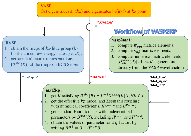
Figure 1: The workflow of VASP2KP to compute the $k\cdot p$ parameters and Landé $g$-factors directly from the VASP wavefunctions.

III.1.2 Spin matrices

By substituting the local operator $\hat{{\bf\it s}}$ for $\hat{F}$ in Eq. (25), the corresponding matrix elements are given explicitly. The first term in Eq. (25) can be calculated by

$$\matrixelement{\widetilde{\alpha}({\bf\it k}_{0})}{\hat{{\bf\it s}}}{\widetilde{\beta}({\bf\it k}_{0})}= \frac{\hbar}{2}\sum_{{\bf\it G}{\bf\it G}^{\prime}\zeta\zeta^{\prime}}{\bf\it\sigma}_{\zeta\zeta^{\prime}}c^{*\alpha{\bf\it k}_{0}}_{\zeta{\bf\it G}}c^{\beta{\bf\it k}_{0}}_{\zeta^{\prime}{\bf\it G}^{\prime}}\delta_{{\bf\it G},{\bf\it G}^{\prime}}$$ (33)

where $\hat{{\bf\it s}}=\frac{\hbar}{2}\hat{{\bf\it\sigma}}$ and the projection matrix can be obtained by

$${\bf\it s}^{a}_{\mu\zeta,\nu\zeta^{\prime}}= \frac{\hbar}{2}\delta_{l_{\mu}l_{\nu}}\delta_{m_{\mu}m_{\nu}}{\bf\it\sigma}_{\zeta\zeta^{\prime}}\int\mathrm{d}rr^{2}\left(R^{a*}_{\mu}R^{a}_{\nu}-\widetilde{R}^{a*}_{\mu}\widetilde{R}^{a}_{\nu}\right)$$ (34)

Finally, by substituting Eqs. (33,34) into Eq. (25), the matrices of the spin $\hat{{\bf\it s}}$ can be obtained in the PAW wavefunctions.

III.1.3 Space group operator matrices

The general (magnetic) space group operator (SGO) is expressed by $F=\{R|{\bf\it v}\}$ or $F=\{TR|{\bf\it v}\}$, which is usually a nonlocal (NL) operator. One should notice that the SGO commutes with $\mathcal{T}$ in Eq. (23). Thus the matrix element can be written as

$$F^{NL}_{mn}= \matrixelement{m({\bf\it k}_{0})}{\hat{F}}{n({\bf\it k}_{0})}=\matrixelement{\widetilde{m}({\bf\it k}_{0})}{\mathcal{T}^{\dagger}\mathcal{T}}{\hat{F}\cdot\widetilde{n}({\bf\it k}_{0})}$$

$$= \langle{\widetilde{m}({\bf\it k}_{0})}|\hat{F}\cdot\widetilde{n}({\bf\it k}_{0})\rangle$$

$$+\sum_{a\mu\nu\zeta}\innerproduct{\widetilde{m}({\bf\it k}_{0})}{\widetilde{p}^{a}_{\mu}\zeta}C^{a}_{\mu,\nu}\innerproduct{\widetilde{p}^{a}_{\nu}\zeta}{\hat{F}\cdot\widetilde{n}({\bf\it k}_{0})},$$ (35)

where

$$C^{a}_{\mu,\nu}=\delta_{l_{\mu}l_{\nu}}\delta_{m_{\mu}m_{\nu}}\int\mathrm{d}rr^{2}\left(R^{a*}_{\mu}R^{a}_{\nu}-\widetilde{R}^{a*}_{\mu}\widetilde{R}^{a}_{\nu}\right)$$ (36)

$$\matrixelement{{\bf\it r},\zeta}{\left\{R|{\bf\it v}\right\}}{\widetilde{\beta}({\bf\it k}_{0})}=\sum_{G}c^{\beta{\bf\it k}_{0}}_{\zeta{\bf\it G}}e^{i({{\bf\it k}_{0}}+{{\bf\it G}})\cdot R^{-1}({{\bf\it r}}-{{\bf\it v}})}$$

$$\matrixelement{{\bf\it r},\zeta}{\left\{TR|{\bf\it v}\right\}}{\widetilde{\beta}({\bf\it k}_{0})}=\eta_{\zeta}\sum_{G}c^{\beta{\bf\it k}_{0}*}_{\overline{\zeta}{\bf\it G}}e^{-i({{\bf\it k}_{0}}+{{\bf\it G}})\cdot R^{-1}({{\bf\it r}}-{{\bf\it v}})}$$

Here, $\eta_{\uparrow}=1$, $\eta_{\downarrow}=-1$, and $\bar{\zeta}$ indicates the opposite of spin $\zeta$. In our convention, the translation ${\bf\it L}$ is expressed by a phase factor of $e^{-i{\bf\it k}_{0}\cdot{\bf\it L}}$. More functions of the patch vasp2mat are presented in Appendix D.

III.2 The python code mat2kp

In this subsection, we give a brief introduction of the main algorithm steps of mat2kp. This code needs the inputs of $\varepsilon_{n}({\bf\it k}_{0})$, ${\bf\it\pi}_{mn}$, ${\bf\it s}_{\alpha\beta}$, $D^{\text{num}}_{\alpha\beta}(R)$ and $D^{\text{std}}_{\alpha\beta}(R)$, which correspond to the EIGENVAL, MAT_Pi.m, MAT_sig.m, MAT_R.m and mat2kp.in files, respectively. The main steps of mat2kp are as follows:

1. Following Sec. II.4, calculate the unitary transformation matrix $U$ satisfying $D^{\text{std}}(R)=U^{\dagger}D^{\text{num}}(R)U$ for $\forall R\in L$.

2. By downfolding processing and using Eqs. (5-8), get the numerical $k\cdot p$ Hamiltonian and Zeeman’s coupling and compute the coefficients numerically under DFT basis, i.e., $H^{kp-\text{num}}$ and $H^{Z-\text{num}}$.

3. Through theory of invariants in Sec. II.3, import the package kdotp-generator and generate the standard $k\cdot p$ Hamiltonian and Zeeman’s coupling with a set of undetermined parameters, $H^{kp-\text{std}}$ and $H^{Z-\text{std}}$, respectively.

4. Obtain the values of $k\cdot p$ parameters and Landé $g$-factors by solving $H^{kp-\text{std}}=U^{-1}H^{kp-\text{num}}U$ and $H^{Z-\text{std}}=U^{-1}H^{Z-\text{num}}U$ in Sec. II.5.

III.3 General steps to get the $k\cdot p$ model and parameters automatically

The general workflow is given in Fig. 1. We will take Bi₂Se₃ as an example for illustration.

1. Run VASP to output the eigenstates $\ket{n({\bf\it k}_{0})}$ ($\ket{\widetilde{n}({\bf\it k}_{0})}$ in WAVECAR) and eigenvalues $\varepsilon_{n}({\bf\it k}_{0})$ (EIGENVAL) at ${\bf\it k}_{0}$ point.

2. Run IRVSP to get the irreps of the aimed low-energy bands (set $\mathcal{A}$), and then obtain the standard matrix representations [$D^{\text{std}}(R)$] of the generators of ${\bf\it k}_{0}$-little group on the Bilbao Crystalline Server (BCS). They are given in “mat2kp.in” (the input file of mat2kp).

   ######## mat2kp.in - Bi2Se3 ########
   Symmetry = {
   ’C3z’ : {
   ’rotation_matrix’:
   Matrix([[-Rational(1,2), -sqrt(3)/2,0],[sqrt(3)/2, -Rational(1,2), 0],[0, 0, 1]]),
   ’repr_matrix’:
   Matrix([[Rational(1,2)-I*sqrt(3)/2,0,0,0],[0,Rational(1,2)+I*sqrt(3)/2,0,0],
    [0,0,Rational(1,2)-I*sqrt(3)/2,0],[0,0,0,Rational(1,2)+I*sqrt(3)/2]]),
   ’repr_has_cc’: False},
   ’C2x’ : {
   ’rotation_matrix’: Matrix([[1, 0, 0],[0, -1, 0],[0, 0, -1]]),
   ’repr_matrix’:
   Matrix([[0,-Rational(1,2)-I*sqrt(3)/2,0,0],[Rational(1,2)-I*sqrt(3)/2,0,0,0],
    [0,0,0,-Rational(1,2)-I*sqrt(3)/2],[0,0,Rational(1,2)-I*sqrt(3)/2,0]]),
   ’repr_has_cc’: False},
   ’P’ : {
   ’rotation_matrix’: Matrix([[-1,0,0],[0, -1, 0],[0, 0, -1]]),
   ’repr_matrix’:
   Matrix([[1,0,0,0],[0,1,0,0],[0,0,-1,0],[0,0,0,-1]]),
   ’repr_has_cc’: False},
   ’T’ : {
   ’rotation_matrix’: eye(3),# Identity Matrix
   ’repr_matrix’: Matrix([[0,1,0,0],[-1,0,0,0],[0,0,0,-1],[0,0,1,0]]),
   ’repr_has_cc’: True}
   }
   # optional parameters
   vaspMAT = ’../Bi2Se3/GMmat’ # the path: to read eigenvalues, Pi, s, and R matrices in this folder.
   order = 2    # Order of the kp model : 2 (default) or 3.
   print_flag = 2 # Where to output results: 1 (screen) or 2 (files, default).
   kpmodel = 1   # Whether to compute Hkp: 0 or 1 (default).
   gfactor = 1   # Whether to compute HZ : 0 or 1 (default).
   log = 1     # Whether to output log files: 0 or 1 (default).
   

3. Run vasp2mat to generate ${\bf\it\pi}_{mn}$ (vmat=11; vmat_name=’Pi’), ${\bf\it s}_{\alpha\beta}$ (vmat=10; vmat_name=’sig’), and generators’ [$D(R)^{\text{num}}_{\alpha\beta}$; vmat=12] matrices directly from the VASP wavefunctions (WAVECAR) by the following settings in “INCAR.mat” files, respectively. These numerical matrix representations are output in MAT_Pi.m, MAT_sig.m, MAT_R.m files. They are in the ‘vaspMAT’ folder (given in mat2kp.in). The vmat_name of the generators should be the same as those given in “mat2kp.in”.

   ######## INCAR.mat - Pi mat. ########
   &vmat_para
   ! soc------------------------
   cfactor=1.0
   socfactor=1.0
   nosoc_inH = .false.
   ! operator------------------
   vmat = 11
   vmat_name = ’Pi’
   vmat_k = 1
   bstart=1, bend=400
   print_only_diagnal = .false.
   /
   

   ######## INCAR.mat - sigma mat. ########
   &vmat_para
   ! soc------------------------
   cfactor=1.0
   socfactor=1.0
   nosoc_inH = .false.
   ! operator------------------
   vmat = 10
   vmat_name = ’sig’
   vmat_k = 1
   bstart=47, bend=50
   print_only_diagnal = .false.
   /
   

   ######## INCAR.mat - C3z / C2x / P / T mat. - Bi2Se3 ########
   &vmat_para
   ! soc------------------------
   cfactor=1.0
   socfactor=1.0
   nosoc_inH = .false.
   ! operator------------------
   vmat = 12
   vmat_name = ’C3z’  /  ’C2x’  /  ’P’   /  ’T’
   vmat_k = 1
   bstart=47, bend=50
   print_only_diagnal = .false.
   ! rotation------------------
   rot_n(:) = 0 0 1   /  1 0 0  /  0 0 1  /  0 0 1
   rot_alpha = 120    /  180    /  0     /  0
   rot_det = 1      /  1     /  -1    /  1
   rot_tau(:) = 0 0 0
   rot_spin2pi = .false.
   time_rev = .false.  /  .false. /  .false. /  .true.
   /
   

4. Run the post-processing python code mat2kp with the input files, to construct the standard $k\cdot p$ Hamiltonian and Zeeman’s coupling, and compute the values of $k\cdot p$ parameters and $g$-factors. The outputs are “kp-parameters.out” and “g-factors.out” files, as pasted below.

   ######## kp-parameters.out ########
   kp Hamiltonian
   ========== Result of kp Hamiltonian ==========
   Matrix([[a1 + a2 + c1*(kx**2 + ky**2) + c2*(kx**2 + ky**2) + c3*kz**2 + c4*kz**2, 0, -I*b2*kz, -b1*(kx*(sqrt(3) + 3*I) + ky*(3 - sqrt(3)*I))/3], [0, a1 + a2 + c1*(kx**2 + ky**2) + c2*(kx**2 + ky**2) + c3*kz**2 + c4*kz**2, b1*(kx*(sqrt(3) - 3*I) + ky*(3 + sqrt(3)*I))/3, I*b2*kz], [I*b2*kz, b1*(kx*(sqrt(3) + 3*I) + ky*(3 - sqrt(3)*I))/3, a1 - a2 + c1*(kx**2 + ky**2) - c2*(kx**2 + ky**2) + c3*kz**2 - c4*kz**2, 0], [-b1*(kx*(sqrt(3) - 3*I) + ky*(3 + sqrt(3)*I))/3, -I*b2*kz, 0, a1 - a2 + c1*(kx**2 + ky**2) - c2*(kx**2 + ky**2) + c3*kz**2 - c4*kz**2]])
   Parameters:
   a1 = 4.8898 ;
   a2 = -0.2244 ;
   b1 = -3.238 ;
   b2 = 2.5562 ;
   c1 = 19.5842 ;
   c2 = 44.4746 ;
   c3 = 1.8117 ;
   c4 = 9.5034 ;
   Error of the linear least square method: 3.93e-06
   Sum of absolute values of numerical zero elements: 6.47e-02
   

   ######## g-factors.out ########
   Zeeman’s coupling
   ========== Result of Zeeman’s coupling ==========
   mu_B/2*Matrix([[Bz*g3 + Bz*g4, g1*(Bx*(1 - sqrt(3)*I/3) + By*(-sqrt(3)/3 - I)) + g2*(Bx*(1 - sqrt(3)*I/3) + By*(-sqrt(3)/3 - I)), 0, 0], [g1*(Bx*(1 + sqrt(3)*I/3) + By*(-sqrt(3)/3 + I)) + g2*(Bx*(1 + sqrt(3)*I/3) + By*(-sqrt(3)/3 + I)), -Bz*g3 - Bz*g4, 0, 0], [0, 0, Bz*g3 - Bz*g4, g1*(Bx*(1 - sqrt(3)*I/3) + By*(-sqrt(3)/3 - I)) + g2*(Bx*(-1 + sqrt(3)*I/3) + By*(sqrt(3)/3 + I))], [0, 0, g1*(Bx*(1 + sqrt(3)*I/3) + By*(-sqrt(3)/3 + I)) + g2*(Bx*(-1 - sqrt(3)*I/3) + By*(sqrt(3)/3 - I)), -Bz*g3 + Bz*g4]])
   Parameters:
   g1 = -0.3244 ;
   g2 = 5.761 ;
   g3 = -7.8904 ;
   g4 = -13.0138 ;
   Error of the linear least square method: 6.11e-08
   Sum of absolute values of numerical zero elements: 4.12e-03
   

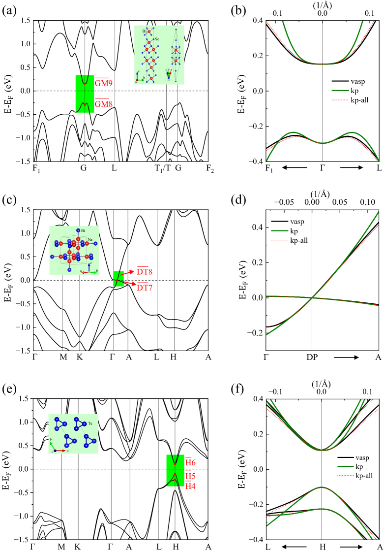
Figure 2: Crystal structure and electronic band structure (VASP) of Bi₂Se₃ (a), Na₃Bi (c) and Te (e). Model dispersions of Bi₂Se₃ (b), Na₃Bi (d) and Te (f) [kp; Eq. (5) and kp-all; Eq. (3)].

IV Applications in materials

In this section, we apply this package to some typical materials, i.e., Bi₂Se₃, Na₃Bi, Te, InAs, and 1H-TMD, to construct the effective models and to compute all the parameters.

IV.1 Four-band model at $\Gamma$ in Bi₂Se₃

As we know, the topological property of Bi₂Se₃ is due to the band inversion at $\Gamma$. By using IRVSP, the lowest conduction band belongs to $\overline{\text{GM}}9$ (twofold degenerate), while the highest valence band belongs to $\overline{\text{GM}}8$ (twofold degenerate), as depicted in Fig. 2(a). Based on these states in the ascending order, the low-energy effective Hamiltonian at $\Gamma$ is constructed automatically. The generators of the $\Gamma$-little group are $\{C_{3z}|0,0,0\}$, $\{C_{2x}|0,0,0\}$, $\{P|0,0,0\}$, and $\{T|0,0,0\}$. Their standard matrix representations are given in TABLE 1, which are needed by the code mat2kp to construct effective models.

To the second order, the $k\cdot p$ Hamiltonian and Zeeman’s coupling are given in Eq. (37), where $\mu_{B}$ is the Bohr magneton ($\sim$ 0.05788 meV/Tesla). After their numerical matrix representations are computed by vasp2mat directly from the VASP wavefunctions, the parameters of $k\cdot p$ Hamiltonian and $g$-factors of Zeeman’s coupling are computed, as shown in TABLE 2. The four-band model’s dispersions are plotted in Fig. 2(b). They fit well with the VASP bands in the vicinity of $\Gamma$. Moreover, the dispersions of the all-band $k\cdot p$ model without downfolding in Eq. (3) are also plotted for comparison (labeled by ‘kp-all’).

$$H^{\text{eff}}({\bf\it k},{\bf\it B})=H^{kp}+H^{Z},$$ (37)

$$H^{kp}=\begin{pmatrix}D_{1}&0&-ib_{2}k_{z}&-\frac{3i+\sqrt{3}}{3}b_{1}k_{-}\\ &D_{1}&\frac{\sqrt{3}-3i}{3}b_{1}k_{+}&ib_{2}k_{z}\\ &&D_{2}&0\\ \dagger&&&D_{2}\end{pmatrix},$$

$$H^{Z}=\frac{\mu_{B}}{2}\begin{pmatrix}h_{1}^{+}B_{z}&h_{2}^{+}B_{+}&0&0\\ &-h_{1}^{+}B_{z}&0&0\\ &&h_{1}^{-}B_{z}&h_{2}^{-}B_{-}\\ \dagger&&&-h_{1}^{-}B_{z}\end{pmatrix},$$

$$D_{1}=a_{1}+a_{2}+(c_{1}+c_{2})k_{+}k_{-}+(c_{3}+c_{4})k_{z}^{2},$$

$$D_{2}=a_{1}-a_{2}+(c_{1}-c_{2})k_{+}k_{-}+(c_{3}-c_{4})k_{z}^{2},$$

$$h_{1}^{\pm}=g_{3}\pm g_{4},h_{2}^{\pm}=\frac{3-\sqrt{3}i}{3}(g_{1}\pm g_{2}),$$

$$k_{\pm}=k_{x}\pm ik_{y},\quad B_{\pm}=B_{x}\pm iB_{y}.$$

Table 1: The matrix representations of ${\rm\overline{GM}}8$ and $\rm{\overline{GM}}9$ irreps at $\Gamma$ are given on BCS server for the generators.

	$\overline{\text{GM}}8$	$\overline{\text{GM}}9$
$\{C_{3z}|0,0,0\}$	$\begin{pmatrix}e^{-\frac{\pi i}{3}}&0\\ 0&e^{\frac{\pi i}{3}}\end{pmatrix}$	$\begin{pmatrix}e^{-\frac{\pi i}{3}}&0\\ 0&e^{\frac{\pi i}{3}}\end{pmatrix}$
$\{C_{2x}|0,0,0\}$	$\begin{pmatrix}0&e^{-\frac{2\pi i}{3}}\\ e^{-\frac{\pi i}{3}}&0\end{pmatrix}$	$\begin{pmatrix}0&e^{-\frac{2\pi i}{3}}\\ e^{-\frac{\pi i}{3}}&0\end{pmatrix}$
$\{P|0,0,0\}$	$\begin{pmatrix}1&0\\ 0&1\end{pmatrix}$	$\begin{pmatrix}-1&0\\ 0&-1\end{pmatrix}$
$\{T|0,0,0\}$	$\begin{pmatrix}0&1\\ -1&0\end{pmatrix}\mathcal{K}$	$\begin{pmatrix}0&-1\\ 1&0\end{pmatrix}\mathcal{K}$

Table 2: The computed values of parameters $\{a_{i},b_{i},c_{i},g_{i}\}$ for Bi₂Se₃ in Eq. (37), obtained from the VASP calculations directly.

$a_{i}$ (eV)	$b_{i}$ (eV$\cdot$Å)	$c_{i}$ (eV$\cdot$Å2)	$g_{i}$
$a_{1}=4.89$	$b_{1}=3.24$	$c_{1}=19.58$	$g_{1}=-0.32$
$a_{2}=-0.22$	$b_{2}=-2.56$	$c_{2}=44.47$	$g_{2}=5.76$
		$c_{3}=1.81$	$g_{3}=-7.90$
		$c_{4}=9.50$	$g_{4}=-13.01$

IV.2 Four-band model at the Dirac point in Na₃Bi

The Dirac semimetal Na₃Bi has a Dirac point (DP: ${\bf\it k}_{D}$) along $\Gamma$-A in Fig. 2(c). It is formed by the crossing of the $\rm\overline{DT}7$-irrep and $\rm\overline{DT}8$-irrep bands. Thus, we construct the effective Hamiltonian at ${\bf\it k}_{D}$. The standard matrix representations are presented in TABLE E1. The $H^{kp}$ and $H^{Z}$ are obtained in Eq. (38) with the computed parameters and $g$-factors in TABLE 3. The four-band $k\cdot p$ model’s dispersions are fitting well with the VASP bands, as shown in Fig. 2(d).

$$H^{kp}= \begin{pmatrix}D_{1}&0&\xi_{-}c_{2}k_{-}^{2}&\Theta_{14}\\ &D_{1}&-i\xi_{-}k_{+}(b_{1}+c_{4}k_{z})&\xi_{+}c_{2}k_{+}^{2}\\ &&D_{2}&0\\ \dagger&&&D_{2}\end{pmatrix},$$ (38)

$$D_{1}=a_{1}+a_{2}+(b_{2}+b_{3})k_{z}+d_{1}^{+}k_{+}k_{-}+d_{2}^{+}k_{z}^{2},$$

$$D_{2}=a_{1}-a_{2}+(b_{2}-b_{3})k_{z}+d_{1}^{-}k_{+}k_{-}+d_{2}^{-}k_{z}^{2},$$

$$d_{1}^{\pm}=c_{1}\pm c_{3},\quad d_{2}^{\pm}=c_{5}\pm c_{6},$$

$$\xi_{\pm}=1\pm\sqrt{3}i,\quad\Theta_{14}=-i\zeta_{+}k_{-}(b_{1}+c_{4}k_{z}),$$

$$H^{Z}= \frac{\mu_{B}}{2}\begin{pmatrix}h_{1}^{+}B_{z}&0&0&\frac{3-\sqrt{3}i}{3}g_{2}B_{-}\\ &-h_{1}^{+}B_{z}&\frac{3+\sqrt{3}i}{3}g_{2}B_{-}&0\\ &&h_{1}^{-}B_{z}&\frac{6+2\sqrt{3}i}{3}g_{1}B_{+}\\ \dagger&&&-h_{1}^{-}B_{z}\end{pmatrix},$$

$$h_{1}^{\pm}=g_{3}\pm g_{4}$$

IV.3 Four-band model at H in Te

Element tellurium is a narrow-gap semiconductor. The direct gap is at H. The low-energy bands at H are the $\rm\overline{H}4$-irrep and $\rm\overline{H}5$-irrep valence bands and $\rm\overline{H}6$-irrep (doubly degenerate) conduction bands. The four-band effective model is constructed accordingly. The standard matrix representations of the generators of the H-little group are given in TABLE E2. The $k\cdot p$ model at H is expressed as

$$H^{kp}_{11}= a_{1}+2a_{2}+a_{3}+(c_{1}+2c_{3}+c_{8})k_{-}k_{+}$$ (39)

$$+(c_{14}+2c_{15}+c_{16})k_{z}^{2},$$

$$H^{kp}_{12}= 2(b_{6}-ib_{7})k_{z},$$

$$H^{kp}_{13}= -\frac{\sqrt{3}}{6}\left[\left(2i\xi_{+}b_{2}+\sqrt{3}i\xi_{+}b_{3}+\sqrt{3}\xi_{+}b_{4}+4ib_{5}\right)k_{+}\right.$$

$$+\left(2i\xi_{+}c_{10}+\sqrt{3}i\xi_{+}c_{11}-\sqrt{3}\xi_{+}c_{12}-4ic_{13}\right)k_{+}k_{z}$$

$$+\left.\left(2i\xi_{+}c_{4}+\sqrt{3}i\xi_{+}c_{5}+\sqrt{3}\xi_{+}c_{6}+4ic_{7}\right)k_{-}^{2}\right],$$

$$H^{kp}_{14}= \frac{\sqrt{3}}{3}\left[\left(2b_{2}+\sqrt{3}b_{3}-\sqrt{3}ib_{4}+\xi_{-}b_{5}\right)k_{-}\right.$$

$$-\left(2c_{10}-\sqrt{3}c_{11}+\sqrt{3}ic_{12}-\xi_{-}c_{13}\right)k_{-}k_{z}$$

$$\left.+\left(2c_{4}+\sqrt{3}c_{5}-\sqrt{3}ic_{6}+\xi_{-}c_{7}\right)k_{+}^{2}\right],$$

$$H^{kp}_{22}= a_{1}-2a_{2}+a_{3}+(c_{1}-2c_{3}+c_{8})k_{-}k_{+}$$

$$+(c_{14}-2c_{15}+c_{16})k_{z}^{2},$$

$$H^{kp}_{23}= \frac{\sqrt{3}}{3}\left[\left(-2b_{2}+\sqrt{3}b_{3}+\sqrt{3}ib_{4}-\xi_{+}b_{5}\right)k_{+}\right.$$

$$+\left(2c_{4}-\sqrt{3}c_{5}-\sqrt{3}ic_{6}+\xi_{+}c_{7}\right)k_{-}^{2}$$

$$\left.+\left(2c_{10}+\sqrt{3}c_{11}+\sqrt{3}ic_{12}-\xi_{+}c_{13}\right)k_{+}k_{z}\right],$$

$$H^{kp}_{24}= \frac{\sqrt{3}}{6}\left[\left(2i\xi_{-}b_{2}-\sqrt{3}i\xi_{-}b_{3}+\sqrt{3}\xi_{-}b_{4}+4ib_{5}\right)k_{-}\right.$$

$$+\left(2i\xi_{-}c_{10}+\sqrt{3}i\xi_{-}c_{11}-\sqrt{3}\xi_{-}c_{12}-4ic_{13}\right)k_{-}k_{z}$$

$$\left.+\left(2i\xi_{-}c_{4}-\sqrt{3}i\zeta_{-}c_{5}-\sqrt{3}\xi_{-}c_{6}+4ic_{7}\right)k_{+}^{2}\right],$$

$$H^{kp}_{33}= H^{kp}_{44}=a_{1}-a_{3}+2b_{8}k_{z}+(c_{1}-c_{8})k_{-}k_{+}$$

$$+(c_{14}-c_{16})k_{z}^{2},$$

$$H^{kp}_{34}= \frac{2\sqrt{3}}{3}i\xi_{-}b_{1}k_{+}+\frac{2\sqrt{3}}{3}i\xi_{-}c_{2}k_{-}^{2}+2\xi_{-}c_{9}k_{+}k_{z}$$

$$\text{with}\quad\xi_{\pm}=1\pm\sqrt{3}i$$

Zeeman’s coupling is expressed by

$$H^{Z}= \frac{\mu_{B}}{2}\begin{pmatrix}0&(g_{6}-ig_{7})B_{z}&h_{1}B_{+}&h_{2}B_{-}\\ &0&h_{3}B_{+}&h_{4}B_{+}\\ &&g_{8}B_{z}&\frac{6+2\sqrt{3}i}{3}g_{1}B_{+}\\ \dagger&&&-g_{8}B_{z}\end{pmatrix},$$ (40)

$$h_{1}= \frac{3-\sqrt{3}i}{3}g_{2}+\frac{\sqrt{3}-i}{2}g_{3}-\frac{\sqrt{3}i+1}{2}g_{4}-\frac{2\sqrt{3}}{3}ig_{5},$$

$$h_{2}= \frac{2\sqrt{3}}{3}g_{2}+g_{3}-ig_{4}+\frac{\sqrt{3}-3i}{3}g_{5},$$

$$h_{3}= -\frac{2\sqrt{3}}{3}g_{2}+g_{3}+ig_{4}-\frac{\sqrt{3}+3i}{3}g_{5},$$

$$h_{4}= \frac{3+\sqrt{3}i}{3}g_{2}-\frac{\sqrt{3}+i}{2}g_{3}-\frac{\sqrt{3}i-1}{2}g_{4}+\frac{2\sqrt{3}}{3}ig_{5}.$$

The computed parameters $\{a_{i},b_{i},c_{i},g_{i}\}$ are presented in TABLE 4. The four-band $k\cdot p$ model’s dispersions agree well with the VASP bands in Fig. 2(f).

Table 3: The computed values of parameters $\{a_{i},b_{i},c_{i},g_{i}\}$ in Eq. (38) for Na₃Bi, obtained from the VASP calculations directly.

$a_{i}$ (eV)	$b_{i}$ (eV$\cdot$Å)	$c_{i}$ (eV$\cdot$Å2)	$g_{i}$
$a_{1}=2.22$	$b_{1}=0.99$	$c_{1}=7.39$	$g_{1}=-3.78$
$a_{2}=0.00$	$b_{2}=1.48$	$c_{2}=-4.02$	$g_{2}=-5.24$
	$b_{3}=-1.69$	$c_{3}=-0.76$	$g_{3}=2.74$
		$c_{4}=7.24$	$g_{4}=8.58$
		$c_{5}=3.17$
		$c_{6}=-4.43$

Table 4: The computed values of parameters in Eqs. (39)-(40) for Te, obtained from the VASP calculations directly.

$a$ (eV)	$b$ (eV$\cdot$Å)	$c$ (eV$\cdot$Å2)	$g$
$a_{1}=5.72$	$b_{1}=-0.16$	$c_{1}=6.13$	$g_{1}=1.52$
$a_{2}=-0.03$	$b_{2}=0.84$	$c_{2}=-0.03$	$g_{2}=-3.12$
$a_{3}=-0.13$	$b_{3}=-1.32$	$c_{3}=2.51$	$g_{3}=-2.64$
	$b_{4}=-1.30$	$c_{4}=4.16$	$g_{4}=0.18$
	$b_{5}=-0.55$	$c_{5}=1.63$	$g_{5}=4.08$
	$b_{6}=0.65$	$c_{6}=-7.48$	$g_{6}=-0.08$
	$b_{7}=-0.98$	$c_{7}=-1.72$	$g_{7}=-8.92$
	$b_{8}=-0.29$	$c_{8}=-5.96$	$g_{8}=-10.84$
		$c_{9}=1.41$
		$c_{10}=-2.56$
		$c_{11}=5.52$
		$c_{12}=-6.40$
		$c_{13}=-1.04$
		$c_{14}=8.47$
		$c_{15}=-0.09$
		$c_{16}=-46.46$

IV.4 Two-band model at $\Gamma$ in InAs

Here, we compute the band structure of the wurtzite (WZ) InAs semiconductor. Since InAs is usually of $n$-type, we consider the $\overline{\rm GM}8$ conduction bands (doubly degenerate) for the electron doped samples. The matrix representations of generators are presented in TABLE E3. The two-conduction-band effective model is constructed in Eq. (41), and the $k\cdot p$ parameters and $g$-factors are computed as listed in TABLE 5. In Fig. 3(f), the splitting of the conduction bands at field 10T is 6.7 meV, indicating an effective $g$-factor of $11.6$. It is consistent with the experimental value in the bulk material Albrecht et al. (2016); Winkler et al. (2017).

$$H^{kp}= a_{1}+\begin{pmatrix}c_{1}k_{+}k_{-}+c_{2}k_{z}^{2}&(1+\sqrt{3}i)b_{1}k_{-}\\ \dagger&c_{1}k_{+}k_{-}+c_{2}k_{z}^{2}\end{pmatrix}$$ (41)

$$H^{Z}= \frac{\mu_{B}}{2}\begin{pmatrix}g_{2}B_{z}&\frac{3-\sqrt{3}i}{3}g_{1}B_{-}\\ \dagger&-g_{2}B_{z}\end{pmatrix}$$

In addition, another effective model for the six valence bands is constructed in Appendix F. Surprisingly, the highest valence bands show a splitting of 19.8 meV under 10T magnetic field in Fig. 3(f), indicating a remarkable effective $g$-factor, being three times of that of the conduction bands.

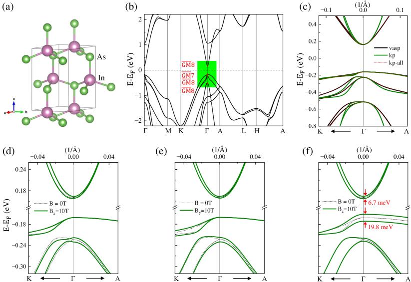
Figure 3: Crystal structure, electronic structure, and $k\cdot p$ band dispersions of InAs. (a) Crystal structure, (b) Electronic band structure (VASP), (c) Model dispersions (kp; Eq. (5) and kp-all; Eq. (3)), and (d-f) the Zeeman effect with magnetic field along $\hat{x}$, $\hat{y}$ and $\hat{z}$ respectively. The splitting due to the magnetic field is depicted explicitly.

Table 5: The computed values of parameters $\{a_{i},b_{i},c_{i},g_{i}\}$ in Eq. (41) in wurtzite InAs are obtained from the VASP calculations directly.

$a_{i}$ (eV)	$b_{i}$ (eV$\cdot$Å)	$c_{i}$ (eV$\cdot$Å2)	$g_{i}$
$a_{1}=4.37$	$b_{1}=-0.20$	$c_{1}=124.41$	$g_{1}=-7.66$
		$c_{2}=123.40$	$g_{2}=-11.60$

IV.5 Two-band model in 1H-TMD monolayers

In 1H-phase transition metal chalcogenide (TMD) monolayers, their direct gaps are at K. The two valence bands at K belong to the $\rm\overline{K}8$-irrep and $\rm\overline{K}11$-irrep, respectively. The standard matrix representations of the generators of the K-little group are given in TABLE E4. The two-band effective models are constructed in Eq. (42) (to the second order), which are plotted in Fig. 4. The computed $k\cdot p$ parameters and $g$-factors are listed in TABLE 6.

$$H^{kp}= a_{1}+\begin{pmatrix}(c_{1}+c_{2})k_{-}k_{+}+a_{2}&0\\ 0&(c_{1}-c_{2})k_{-}k_{+}-a_{2}\end{pmatrix},$$ (42)

$$H^{Z}= \frac{\mu_{B}}{2}B_{z}\begin{pmatrix}g_{1}+g_{2}&0\\ 0&g_{1}-g_{2}\end{pmatrix}.$$

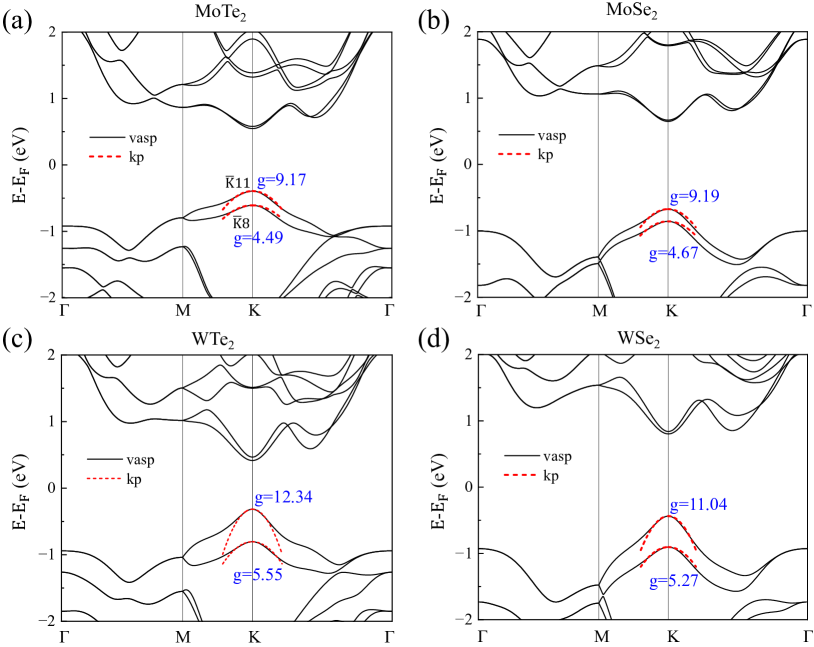
Figure 4: Electronic structures and $k\cdot p$ band dispersions of 1H-TMD monolayers. (a) MoTe₂, (b) MoSe₂, (c) WTe₂, (d) WSe₂.

Table 6: The computed values of parameters $\{a_{i},b_{i},c_{i},g_{i}\}$ in Eq. (42) for 1H-TMD monolayers, obtained from the VASP calculations.

	MoTe2	MoSe2	WTe2	WSe2
$a_{1}$ (eV)	$-1.92$	$-2.93$	$-1.79$	$-2.75$
$a_{2}$ (eV)	$-0.11$	$-0.09$	$-0.24$	$-0.23$
$c_{1}$ (eV$\cdot$Å2)	$-3.83$	$-3.89$	$-8.06$	$-6.48$
$c_{2}$ (eV$\cdot$Å2)	$0.60$	$0.47$	$2.75$	$1.73$
$g_{1}$	$6.82$	$6.92$	$8.94$	$8.16$
$g_{2}$	$-2.34$	$-2.26$	$-3.40$	$-2.88$

Table 7: The computed effective $g$-factors for the two conduction/valence bands only in Bi₂Se₃, Te, InAs, and 1H-TMD. The conduction bands of Te have the larger $g$-factor than the valence bands. The 1st valence (v₁) band has the larger $g$-factor than the 2nd valence band (v₂) in 1H-TMD.

	band	$|g_{z}|$	$|g_{\perp}|$	experiment
Bi2Se3	c	$20.52$	$14.9$	$32$,$23$ Köhler and Wöchner (1975)
Te	c	$6.40$	$3.04$
WZ-InAs	c	$11.60$	$7.66$	$13$ Björk et al. (2005)
MoTe2	v1/v2	$9.17$/$4.49$
MoSe2	v1/v2	$9.19$/$4.67$
WTe2	v1/v2	$12.34$/$5.55$
WSe2	v1/v2	$11.04$/$5.27$		$12.2$ Förste et al. (2020)
WSe2	c1/c2	$1.36$/$6.95$		$1.72$/$7.68$ Förste et al. (2020)

V Discussion

In this work, we develop an open-source package VASP2KP to construct the $k\cdot p$ Hamiltonian and Zeeman’s coupling, and to compute the $k\cdot p$ parameters and Landé $g$-factors from the VASP calculations directly. By applying this package in many typical materials, we get $k\cdot p$ effective models, whose band dispersions are in good agreement with the VASP data around the specific wave vector in the Brillouin zone. As the orbital contribution between the low-energy bands is usually remarkable (due to the small energy difference), the computed $g$-factor is not accurate in the multiple-band model. Thus, we recompute the effective $g$-factor for the two conduction bands only in Bi₂Se₃ and Te. The recomputed values are mainly consistent with the previous experimental data listed in TABLE 7. We reveal that the conduction bands of Te have the larger $g$-factor than the valence bands, and the 1st valence band has the larger $g$-factor than the 2nd valence band in 1H-TMD monolayers. Our results indicate that VASP2KP has the capabilities to handle more materials.

The obtained models provide the effective masses and $g$-factors, which are important physical quantities of the materials. The minor discrepancy from the experimental data is due to the non-precise band gap in the DFT calculations. To improve these parameters, one can use our code in the hybrid functionals or $GW$ calculations. For the new synthesized or predicted materials, for which there is no experimental data available, our code can be used to predict reliable parameters. In conclusion, VASP2KP Zhang et al. (2023b) would be widely used in the Materials Science.

Appendix A Löwdin partitioning theory to obtain $k\cdot p$ Hamiltonian

The Löwdin partitioning theory, also called as quasi-degenerate perturbation, is really a useful and important method to make an approximation to simplify the Hamiltonian by reducing the dimension. The main idea of it is to introduce an anti-Hermitian matrix $S$, which can transform the origin Hamiltonian matrix $H$ (such as $k\cdot p$ Hamiltonian $H^{kp}$ defined by Eq. (3)) to the optimal Hamiltonian matrix $\widetilde{H}$, which is expressed by

$$\widetilde{H}=e^{-S}He^{S}$$ (A.1)

It is obvious that $\widetilde{H}$ has the same eigenvalues as $H$, thus making the corresponding bands all the same. Moreover, $\widetilde{H}$ is expected to be block diagonal, as shown in Fig. A1, where $\mathcal{A}$ corresponds to the subspace of the bands of interest and $\mathcal{B}$ corresponds to the subspace of other bands. After this transformation, we can directly use the matrix block corresponding to $\mathcal{A}$ to replace the original Hamiltonian matrix. However, it is difficult to get the analytic or accurate matrix $S$, so we must use the perturbation expansion method to find the series solution.

First, suppose that the Hamiltonian $H=H_{0}+H^{\prime}$, where $H_{0}$ is a diagonal matrix, which is the main part of the Hamiltonian while $H^{\prime}$ can be treated as a perturbation. For instance, the $k\cdot p$ Hamiltonian $H^{kp}$ can be the sum of the diagonal matrix whose diagonal elements are the eigenvalues $\epsilon_{n}({{\bf\it k}}_{0})$

$$(H_{0}^{kp})_{mn}=\left(\epsilon_{n}({{\bf\it k}}_{0})+\frac{\hbar^{2}k^{2}}{2m}\right)\delta_{mn}$$ (A.2)

and the perturbation terms

$$H^{\prime kp}_{mn}=\frac{\hbar}{m}{{\bf\it\pi}}_{mn}\cdot{{\bf\it k}}\ ,\ (m\neq n)$$ (A.3)

with small ${{\bf\it k}}$. Furthermore, $H^{\prime}$ can be separated as the sum of $H_{1}$ and $H_{2}$ which only have nonzero elements in and between the subspaces $\mathcal{A}$ and $\mathcal{B}$, respectively, as shown in Fig. A2. Therefore, we can rewrite the origin Hamiltonian as

$$H=H_{0}+H_{1}+H_{2}$$ (A.4)

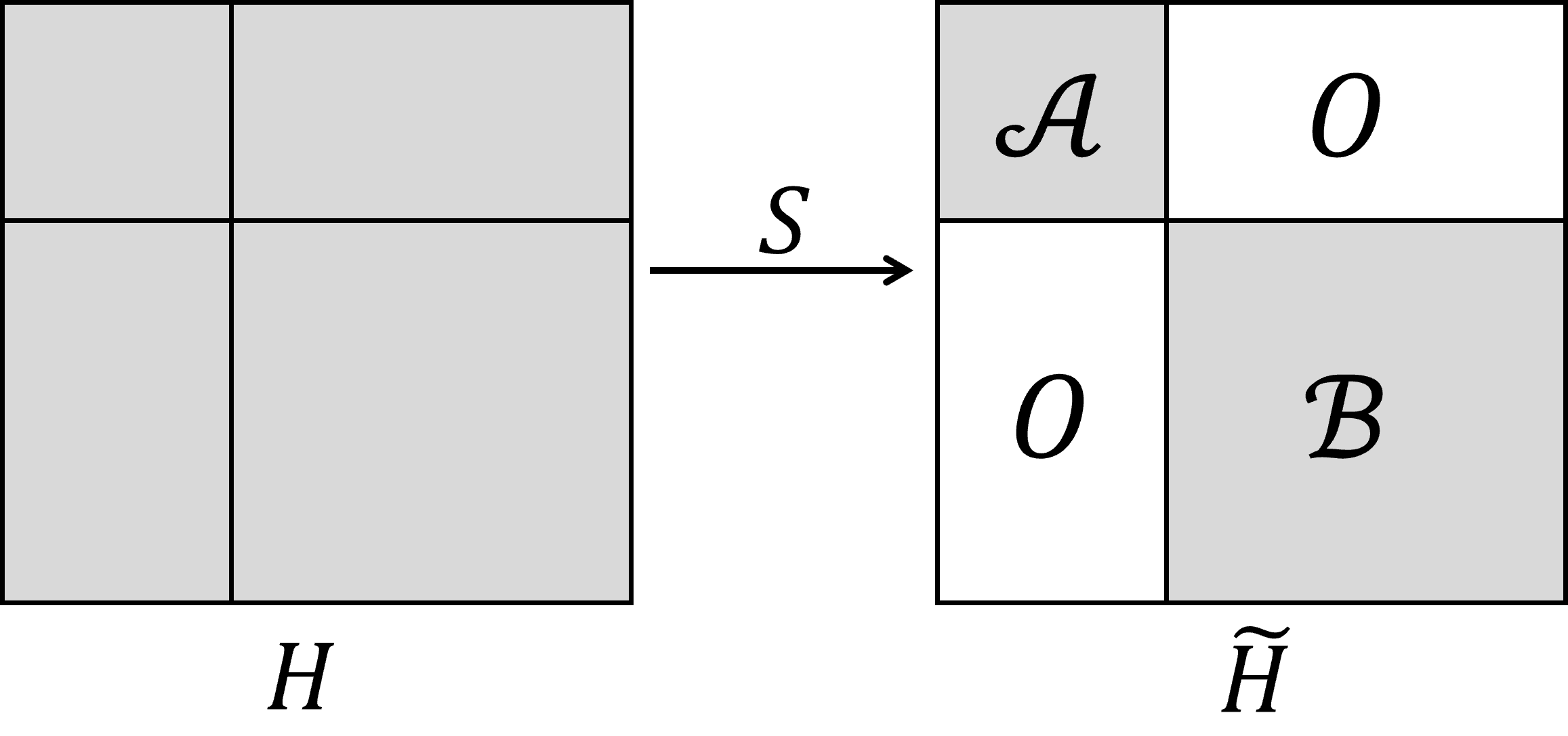
Figure A1: Transform the original Hamiltonian $H$ to the optimal Hamiltonian $\widetilde{H}$. The gray parts represent nontrivial matrix elements while the white parts represent trivial matrix elements (zero elements).

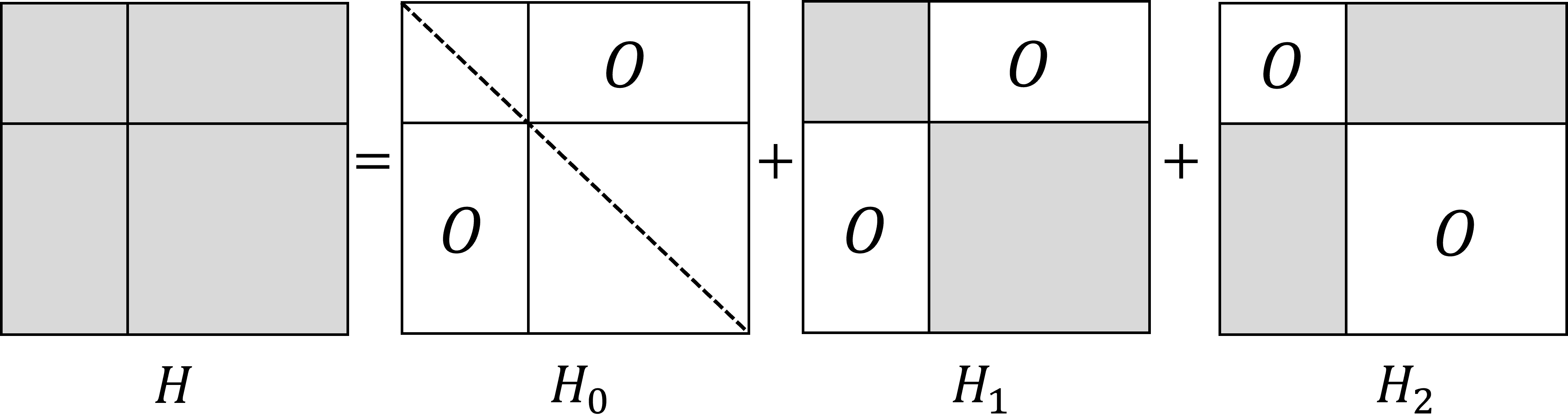
Figure A2: The schematic of $H$, $H_{0}$, $H_{1}$ and $H_{2}$. The gray parts represent nontrivial matrix elements while the white parts represent trivial matrix elements.

We suppose that the matrix $S$ is anti-Hermitian and in the same shape as $H_{2}$ (only has nonzero matrix elements between subspaces $\mathcal{A}$ and $\mathcal{B}$), making $e^{S}$ a unitary matrix. It is simple to find that $[H_{1},S]$ is in the same shape as $H_{2}$ and $[H_{2},S]$ is in the same shape as $H_{1}$, no matter what $H_{1}$ and $H_{2}$ are. According to the Baker–Campbell–Hausdorff formula, Eq. (A.1) can be rewritten as

$$\widetilde{H}=\sum_{i=0}^{+\infty}\frac{1}{i!}[H,S]^{(i)}$$ (A.5)

$$= \sum_{i=0}^{+\infty}\frac{1}{(2i)!}[H_{0}+H_{1},S]^{(2i)}+\sum_{i=0}^{+\infty}\frac{1}{(2i+1)!}[H_{2},S]^{(2i+1)}+\sum_{i=0}^{+\infty}\frac{1}{(2i+1)!}[H_{0}+H_{1},S]^{(2i+1)}+\sum_{i=0}^{+\infty}\frac{1}{(2i)!}[H_{2},S]^{(2i)}$$

The sum of first two terms of Eq. (A.5) is block diagonal in the same shape as $H_{1}$, which is denoted by

$$\widetilde{H}_{D}=\sum_{i=0}^{+\infty}\frac{1}{(2i)!}[H_{0}+H_{1},S]^{(2i)}+\sum_{i=0}^{+\infty}\frac{1}{(2i+1)!}[H_{2},S]^{(2i+1)}$$ (A.6)

and the sum of last two terms of Eq. (A.5) is non-block diagonal in the same shape as $H_{2}$, which is denoted by

$$\widetilde{H}_{N}=\sum_{i=0}^{+\infty}\frac{1}{(2i+1)!}[H_{0}+H_{1},S]^{(2i+1)}+\sum_{i=0}^{+\infty}\frac{1}{(2i)!}[H_{2},S]^{(2i)}$$ (A.7)

To make $\widetilde{H}$ block diagonal, we have $\widetilde{H}_{N}=0$. Use the ansatz that $S$ can be expanded as

$$S=S^{(1)}+S^{(2)}+S^{(3)}+\cdots$$ (A.8)

Extract the small quantities of each order in $H_{N}$ and let them be 0:

1st order

$$[H_{0},S^{(1)}]+H_{2}=0$$ (A.9)

2nd order

$$[H_{0},S^{(2)}]+[H_{1},S^{(1)}]=0$$ (A.10)

3rd order

$$[H_{0},S^{(3)}]+\frac{1}{6}[H_{0},S^{(1)}]^{(3)}+[H_{1},S^{(2)}]+\frac{1}{2}[H_{2},S^{(1)}]^{(2)}=0$$ (A.11)

$\cdots$

By solving Eqs. (A.9)-(A.11), the matrix elements of $S^{(i)}$ can be written as

$$\left\{\begin{aligned} &S^{(1)}_{\alpha l}=-\frac{H^{\prime}_{\alpha l}}{E_{\alpha}-E_{l}}\\ &S_{\alpha l}^{(2)}=\frac{1}{E_{\alpha}-E_{l}}\left[\sum_{\alpha^{\prime}\in\mathcal{A}}\frac{H^{\prime}_{\alpha\alpha^{\prime}}H^{\prime}_{\alpha^{\prime}l}}{E_{\alpha^{\prime}}-E_{l}}-\sum_{l^{\prime}\in\mathcal{B}}\frac{H^{\prime}_{\alpha l^{\prime}}H^{\prime}_{l^{\prime}l}}{E_{\alpha}-E_{l^{\prime}}}\right]\\ &\begin{aligned} S_{\alpha l}^{(3)}=&\frac{1}{E_{\alpha}-E_{l}}\\ \times&\left[-\sum_{\alpha^{\prime},\alpha^{\prime\prime}\in\mathcal{A}}\frac{H^{\prime}_{\alpha\alpha^{\prime\prime}}H^{\prime}_{\alpha^{\prime\prime}\alpha^{\prime}}H^{\prime}_{\alpha^{\prime}l}}{\left(E_{\alpha^{\prime\prime}}-E_{l}\right)\left(E_{\alpha^{\prime}}-E_{l}\right)}-\sum_{l^{\prime},l^{\prime\prime}\in\mathcal{B}}\frac{H^{\prime}_{\alpha l^{\prime}}H^{\prime}_{l^{\prime}l^{\prime\prime}}H^{\prime}_{l^{\prime\prime}l}}{\left(E_{\alpha}-E_{l^{\prime\prime}}\right)\left(E_{\alpha}-E_{l^{\prime}}\right)}\right.\\ &+\sum_{l^{\prime}\in\mathcal{B},\alpha^{\prime}\in\mathcal{A}}\frac{H^{\prime}_{\alpha\alpha^{\prime}}H^{\prime}_{\alpha^{\prime}l^{\prime}}H^{\prime}_{l^{\prime}l}}{\left(E_{\alpha^{\prime}}-E_{l}\right)\left(E_{\alpha^{\prime}}-E_{l^{\prime}}\right)}+\sum_{l^{\prime}\in\mathcal{B},\alpha^{\prime}\in\mathcal{A}}\frac{H^{\prime}_{\alpha\alpha^{\prime}}H^{\prime}_{\alpha^{\prime}l^{\prime}}H^{\prime}_{l^{\prime}l}}{\left(E_{m}-E_{l^{\prime}}\right)\left(E_{\alpha^{\prime}}-E_{l^{\prime}}\right)}\\ &+\frac{1}{3}\sum_{l^{\prime}\in\mathcal{B},\alpha^{\prime}\in\mathcal{A}}\frac{H^{\prime}_{\alpha l^{\prime}}H^{\prime}_{l^{\prime}\alpha^{\prime}}H^{\prime}_{\alpha^{\prime}l}}{\left(E_{\alpha^{\prime}}-E_{l^{\prime}}\right)\left(E_{\alpha^{\prime}}-E_{l}\right)}+\frac{1}{3}\sum_{l^{\prime}\in\mathcal{B},\alpha^{\prime}\in\mathcal{A}}\frac{H^{\prime}_{\alpha l^{\prime}}H^{\prime}_{l^{\prime}\alpha^{\prime}}H^{\prime}_{\alpha^{\prime}l}}{\left(E_{\alpha}-E_{l^{\prime}}\right)\left(E_{\alpha^{\prime}}-E_{l^{\prime}}\right)}\left.+\frac{2}{3}\sum_{l^{\prime}\in\mathcal{B},\alpha^{\prime}\in\mathcal{A}}\frac{H^{\prime}_{\alpha l^{\prime}}H^{\prime}_{l^{\prime}\alpha^{\prime}}H^{\prime}_{\alpha^{\prime}l}}{\left(E_{\alpha}-E_{l^{\prime}}\right)\left(E_{\alpha^{\prime}}-E_{l}\right)}\right]\end{aligned}\\ &\cdots=\cdots\end{aligned}\right.$$ (A.12)

where $\alpha\in\mathcal{A}$ and $l\in\mathcal{B}$. This matrix $S$ makes $\widetilde{H}_{N}=0$ so that $\widetilde{H}=\widetilde{H}_{D}$. After obtaining the matrix $S$, we can directly obtain the optimal Hamiltonian by Eq. (A.6), which is expressed by

$$\widetilde{H}=\widetilde{H}^{(0)}+\widetilde{H}^{(1)}+\widetilde{H}^{(2)}+\widetilde{H}^{(3)}+\cdots$$ (A.13)

where

$$\left\{\begin{aligned} H_{\alpha\alpha^{\prime}}^{(0)}=&H_{\alpha\alpha^{\prime}}^{0}\\ H_{\alpha\alpha^{\prime}}^{(1)}=&H_{\alpha\alpha^{\prime}}^{\prime}\\ H_{\alpha\alpha^{\prime}}^{(2)}=&\frac{1}{2}\sum_{l\in\mathcal{B}}H_{\alpha l}^{\prime}H_{l\alpha^{\prime}}^{\prime}\left[\frac{1}{E_{\alpha}-E_{l}}+\frac{1}{E_{\alpha^{\prime}}-E_{l}}\right]\\ H_{\alpha\alpha^{\prime}}^{(3)}=&-\frac{1}{2}\sum_{l\in\mathcal{B},\alpha^{\prime\prime}\in\mathcal{A}}\left[\frac{H_{\alpha l}^{\prime}H_{l\alpha^{\prime\prime}}^{\prime}H_{\alpha^{\prime\prime}\alpha^{\prime}}^{\prime}}{\left(E_{\alpha^{\prime}}-E_{l}\right)\left(E_{\alpha^{\prime\prime}}-E_{l}\right)}+\frac{H_{\alpha\alpha^{\prime\prime}}^{\prime}H_{\alpha^{\prime\prime}l}^{\prime}H_{l\alpha^{\prime}}^{\prime}}{\left(E_{\alpha}-E_{l}\right)\left(E_{\alpha^{\prime\prime}}-E_{l}\right)}\right]\\ &+\frac{1}{2}\sum_{l,l^{\prime}\in\mathcal{B}}H_{\alpha l}^{\prime}H_{ll^{\prime}}^{\prime}H_{l^{\prime}\alpha^{\prime}}^{\prime}\left[\frac{1}{\left(E_{\alpha}-E_{l}\right)\left(E_{\alpha}-E_{l^{\prime}}\right)}+\frac{1}{\left(E_{\alpha^{\prime}}-E_{l}\right)\left(E_{\alpha^{\prime}}-E_{l^{\prime}}\right)}\right]\\ \cdots=\cdots\end{aligned}\right.$$ (A.14)

Up to now, we have already obtained the optimal Hamiltonian. In the case of $k\cdot p$ Hamiltonian, by substituting Eq. (A.2) and Eq. (A.3) into Eq. (A.14), we can obtain

$$\left\{\begin{aligned} &H^{kp(0)}_{\alpha\beta}=\left(\epsilon_{\alpha}({{\bf\it k}}_{0})+\frac{\hbar^{2}k^{2}}{2m}\right)\delta_{\alpha\beta}\\ &H^{kp(1)}_{\alpha\beta}=\frac{\hbar}{m}{{\bf\it\pi}}_{\alpha\beta}\cdot{{\bf\it k}}\\ &H^{kp(2)}_{\alpha\beta}=\frac{\hbar^{2}}{2m^{2}}\sum_{l\in\mathcal{B}}\sum_{ij}\left[\frac{1}{\epsilon_{\alpha}({{\bf\it k}}_{0})-\epsilon_{l}({{\bf\it k}}_{0})}+\frac{1}{\epsilon_{\beta}({{\bf\it k}}_{0})-\epsilon_{l}({{\bf\it k}}_{0})}\right]\pi^{i}_{\alpha l}\pi^{j}_{l\beta}k^{i}k^{j}\\ &\begin{aligned} H^{kp(3)}_{\alpha\beta}=-\frac{\hbar^{3}}{2m^{3}}\sum_{ijq}\left\{\sum_{l\in\mathcal{B},\gamma\in\mathcal{A}}\left[\frac{\pi^{i}_{\alpha l}\pi^{j}_{l\gamma}\pi^{q}_{\gamma\beta}}{(\epsilon_{\beta}({{\bf\it k}}_{0})-\epsilon_{l}({{\bf\it k}}_{0}))(\epsilon_{\gamma}({{\bf\it k}}_{0})-\epsilon_{l}({{\bf\it k}}_{0}))}+\frac{\pi^{i}_{\alpha\gamma}\pi^{j}_{\gamma l}\pi^{q}_{l\beta}}{(\epsilon_{\alpha}({{\bf\it k}}_{0})-\epsilon_{l}({{\bf\it k}}_{0}))(\epsilon_{\gamma}({{\bf\it k}}_{0})-\epsilon_{l}({{\bf\it k}}_{0}))}\right]\right.\\ \left.-\sum_{l,l^{\prime}\in\mathcal{B}}\left[\frac{1}{(\epsilon_{\alpha}({{\bf\it k}}_{0})-\epsilon_{l}({{\bf\it k}}_{0}))(\epsilon_{\alpha}({{\bf\it k}}_{0})-\epsilon_{l^{\prime}}({{\bf\it k}}_{0}))}+\frac{1}{(\epsilon_{\beta}({{\bf\it k}}_{0})-\epsilon_{l}({{\bf\it k}}_{0}))(\epsilon_{\beta}({{\bf\it k}}_{0})-\epsilon_{l^{\prime}}({{\bf\it k}}_{0}))}\right]\pi^{i}_{\alpha l}\pi^{j}_{ll^{\prime}}\pi^{q}_{l^{\prime}\beta}\right\}k^{i}k^{j}k^{q}\end{aligned}\end{aligned}\right.$$ (A.15)

Therefore, the $k\cdot p$ Hamiltonian of order 2 is the sum of $H^{kp(0)}$, $H^{kp(1)}$ and $H^{kp(2)}$, which is equal to Eq. (4). Moreover, the $k\cdot p$ Hamiltonian of order 3 can be expressed by

$$H^{kp(\leq 3)}_{\alpha\beta}$$ (A.16)

$$= \left(\epsilon_{\alpha}({{\bf\it k}}_{0})+\frac{\hbar^{2}k^{2}}{2m}\right)\delta_{\alpha\beta}+\frac{\hbar}{m}{{\bf\it\pi}}_{\alpha\beta}\cdot{{\bf\it k}}+\frac{\hbar^{2}}{2m^{2}}\sum_{l\in\mathcal{B}}\sum_{ij}\left[\frac{1}{\epsilon_{\alpha}({{\bf\it k}}_{0})-\epsilon_{l}({{\bf\it k}}_{0})}+\frac{1}{\epsilon_{\beta}({{\bf\it k}}_{0})-\epsilon_{l}({{\bf\it k}}_{0})}\right]\pi^{i}_{\alpha l}\pi^{j}_{l\beta}k^{i}k^{j}$$

$$-\frac{\hbar^{3}}{2m^{3}}\sum_{ijq}\left\{\sum_{l\in\mathcal{B},\gamma\in\mathcal{A}}\left[\frac{\pi^{i}_{\alpha l}\pi^{j}_{l\gamma}\pi^{q}_{\gamma\beta}}{(\epsilon_{\beta}({{\bf\it k}}_{0})-\epsilon_{l}({{\bf\it k}}_{0}))(\epsilon_{\gamma}({{\bf\it k}}_{0})-\epsilon_{l}({{\bf\it k}}_{0}))}+\frac{\pi^{i}_{\alpha\gamma}\pi^{j}_{\gamma l}\pi^{q}_{l\beta}}{(\epsilon_{\alpha}({{\bf\it k}}_{0})-\epsilon_{l}({{\bf\it k}}_{0}))(\epsilon_{\gamma}({{\bf\it k}}_{0})-\epsilon_{l}({{\bf\it k}}_{0}))}\right]\right.$$

$$\qquad\quad\left.-\sum_{l,l^{\prime}\in\mathcal{B}}\left[\frac{1}{(\epsilon_{\alpha}({{\bf\it k}}_{0})-\epsilon_{l}({{\bf\it k}}_{0}))(\epsilon_{\alpha}({{\bf\it k}}_{0})-\epsilon_{l^{\prime}}({{\bf\it k}}_{0}))}+\frac{1}{(\epsilon_{\beta}({{\bf\it k}}_{0})-\epsilon_{l}({{\bf\it k}}_{0}))(\epsilon_{\beta}({{\bf\it k}}_{0})-\epsilon_{l^{\prime}}({{\bf\it k}}_{0}))}\right]\pi^{i}_{\alpha l}\pi^{j}_{ll^{\prime}}\pi^{q}_{l^{\prime}\beta}\right\}k^{i}k^{j}k^{q}$$

Appendix B Derivation of Zeeman’s coupling

It is easy to compute the commutator $[\partial^{i},A^{j}]$ as

$$[\partial^{i},A^{j}]\phi=\partial^{i}(A^{j}\phi)-A^{j}\partial^{i}\phi=(\partial^{i}A^{j})\phi+A^{j}\partial^{i}\phi-A^{j}\partial^{i}\phi=(\partial^{i}A^{j})\phi$$ (B.1)

or in a simple form

$$[\partial^{i},A^{j}]=\partial^{i}A^{j}.$$ (B.2)

In addition, the components of the magnetic field can be expressed by

$$B_{k}=(\nabla\times{\bf\it A})\cdot{{\bf\it e}}^{k}=\sum_{lmn}\epsilon_{lmn}\partial^{m}A^{n}{{\bf\it e}^{l}}\cdot{{\bf\it e}}^{k}=\sum_{lmn}\epsilon_{lmn}\partial^{m}A^{n}\delta_{lk}=\sum_{mn}\epsilon_{kmn}\partial^{m}A^{n}$$ (B.3)

where $\epsilon_{lmn}$ is the Levi-Civita symbol and $A$ is the magnetic vector potential. Therefore, we can establish the relation that

$$\sum_{k}\epsilon^{ijk}B_{k} =\sum_{mnk}\epsilon^{ijk}\epsilon_{kmn}\partial^{m}A^{n}=\sum_{mn}\left(\sum_{k}\epsilon^{ijk}\epsilon_{kmn}\right)\partial^{m}A^{n}=\sum_{mn}(\delta_{im}\delta_{jn}-\delta_{in}\delta_{jm})\partial^{m}A^{n}=\partial^{i}A^{j}-\partial^{j}A^{i}$$ (B.4)

Therefore, we can obtain the relation in Sec. II.2 that

$$\left[-i\hbar\partial^{i}+eA^{i},-i\hbar\partial^{j}+eA^{j}\right]=-ie\hbar(\left[\partial^{i},A^{j}\right]-\left[\partial^{j},A^{i}\right])=-i\hbar e(\partial^{i}A^{j}-\partial^{j}A^{i})=-i\hbar e\sum_{k}\epsilon^{ijk}B_{k}$$ (B.5)

Furthermore, after replacing $k^{i}$ by $-i\hbar\partial^{i}+eA^{i}$ (Peierls substitution) in Eq. (4), the last summation can be transformed as

$$\sum_{ij}\pi^{i}_{\alpha l}\pi^{j}_{l\beta}(-i\hbar\partial^{i}+eA^{i})(-i\hbar\partial^{j}+eA^{j})$$ (B.6)

$$= \sum_{ij}\pi^{i}_{\alpha l}\pi^{j}_{l\beta}\left(\frac{1}{2}\left[-i\hbar\partial^{i}+eA^{i},-i\hbar\partial^{j}+eA^{j}\right]+\frac{1}{2}\left\{-i\hbar\partial^{i}+eA^{i},-i\hbar\partial^{j}+eA^{j}\right\}\right)$$

$$= -\frac{i\hbar e}{2}\sum_{ijk}\pi^{i}_{\alpha l}\pi^{j}_{l\beta}\epsilon^{ijk}B_{k}+\frac{\hbar^{2}}{2}\sum_{ij}\pi^{i}_{\alpha l}\pi^{j}_{l\beta}\left(-i\partial^{i}+\frac{e}{\hbar}A^{i}\right)\left(-i\partial^{j}+\frac{e}{\hbar}A^{j}\right)+\frac{\hbar^{2}}{2}\sum_{ij}\pi^{i}_{\alpha l}\pi^{j}_{l\beta}\left(-i\partial^{j}+\frac{e}{\hbar}A^{j}\right)\left(-i\partial^{i}+\frac{e}{\hbar}A^{i}\right)$$

$$= -\frac{i\hbar e}{2}\sum_{ijk}\pi^{i}_{\alpha l}\pi^{j}_{l\beta}\epsilon^{ijk}B_{k}+\frac{\hbar^{2}}{2}\sum_{ij}\pi^{i}_{\alpha l}\pi^{j}_{l\beta}\left(-i\partial^{i}+\frac{e}{\hbar}A^{i}\right)\left(-i\partial^{j}+\frac{e}{\hbar}A^{j}\right)+\frac{\hbar^{2}}{2}\sum_{ij}\pi^{j}_{\alpha l}\pi^{i}_{l\beta}\left(-i\partial^{i}+\frac{e}{\hbar}A^{i}\right)\left(-i\partial^{j}+\frac{e}{\hbar}A^{j}\right)$$

$$= -\frac{i\hbar e}{2}\sum_{ijk}\pi^{i}_{\alpha l}\pi^{j}_{l\beta}\epsilon^{ijk}B_{k}+\hbar^{2}\sum_{ij}\frac{\pi^{i}_{\alpha l}\pi^{j}_{l\beta}+\pi^{j}_{\alpha l}\pi^{i}_{l\beta}}{2}\left(-i\partial^{i}+\frac{e}{\hbar}A^{i}\right)\left(-i\partial^{j}+\frac{e}{\hbar}A^{j}\right)$$

The Hamiltonian of Zeeman’s coupling is the gauge independent part in Eq. (4) (after Peierls substitution), which is expressed as

$$H^{Z}_{\alpha\beta}=\frac{\mu_{B}}{\hbar}\left({{\bf\it L}}_{\alpha\beta}+2{{\bf\it s}}_{\alpha\beta}\right)\cdot{{\bf\it B}}$$ (B.7)

where

$$L_{\alpha\beta}^{k}=-\frac{i\hbar}{2m}\sum_{l\in\mathcal{B}}\sum_{ij}\epsilon^{ijk}\pi^{i}_{\alpha l}\pi^{j}_{l\beta}\left(\frac{1}{\epsilon_{\alpha}({{\bf\it k}}_{0})-\epsilon_{l}({{\bf\it k}}_{0})}+\frac{1}{\epsilon_{\beta}({{\bf\it k}}_{0})-\epsilon_{l}({{\bf\it k}}_{0})}\right)$$ (B.8)

and $\frac{2}{\hbar}\mu_{B}{{\bf\it s}}\cdot{{\bf\it B}}$ is the Zeemans’s coupling of the bare electron. In addition, the gauge dependent part in Eq. (4) (after Peierls substitution) is expressed by

$$H^{kp}_{\alpha\beta}=\epsilon_{\alpha}({{\bf\it k}}_{0})\delta_{\alpha\beta}+\frac{\hbar}{m}{{\bf\it\pi}}_{\alpha\beta}\cdot\left(-i\nabla+\frac{e}{\hbar}{{\bf\it A}}\right)+\sum_{ij}M_{\alpha\beta}^{ij}\left(-i\partial^{i}+\frac{e}{\hbar}A^{i}\right)\left(-i\partial^{j}+\frac{e}{\hbar}A^{j}\right)$$ (B.9)

where

$$\begin{aligned} M_{\alpha\beta}^{ij}=\frac{\hbar^{2}}{2m}\delta_{\alpha\beta}\delta_{ij}+\frac{\hbar^{2}}{4m^{2}}\sum_{l\in\mathcal{B}}\left(\pi^{i}_{\alpha l}\pi^{j}_{l\beta}+\pi^{j}_{\alpha l}\pi^{i}_{l\beta}\right)\left(\frac{1}{\epsilon_{\alpha}({{\bf\it k}}_{0})-\epsilon_{l}({{\bf\it k}}_{0})}+\frac{1}{\epsilon_{\beta}({{\bf\it k}}_{0})-\epsilon_{l}({{\bf\it k}}_{0})}\right)\end{aligned}.$$ (B.10)

The Eqs. (B.7)-(B.10) are the same as Eqs. (5)-(8).

Appendix C Construction of the coefficient matrix $Q$ for finding the unitary transformation $U$

Only the generators of the group $L$ should be taken into account when finding the unitary transformation matrix $U$. $T$ is an anti-unitary generator, while $S$ are the unitary generators. The Eq. (17) can be rewritten as

$$D^{\text{num}}(S)U-UD^{\text{std}}(S)=\mathcal{O}$$ (C.1)

$$D^{\text{num}}(T)U^{*}-UD^{\text{std}}(T)=\mathcal{O}$$ (C.2)

where $\mathcal{O}$ is a zero matrix. The matrices $U$, $D^{\text{std}}(R)$ and $D^{\text{num}}(R)$ are complex, so we can consider the real parts and the imaginary parts separately, thus transforming Eqs. (C.1)-(C.2) into

$$\left\{\begin{aligned} D^{\text{num}}_{r}(S)U_{r}-U_{r}D^{\text{std}}_{r}(S)-D^{\text{num}}_{i}(S)U_{i}+U_{i}D^{\text{std}}_{i}(S)=\mathcal{O}\\ D^{\text{num}}_{i}(S)U_{r}-U_{r}D^{\text{std}}_{i}(S)+D^{\text{num}}_{r}(S)U_{i}-U_{i}D^{\text{std}}_{r}(S)=\mathcal{O}\end{aligned}\right.$$ (C.3)

and

$$\left\{\begin{aligned} D^{\text{num}}_{r}(T)U_{r}-U_{r}D^{\text{std}}_{r}(T)+D^{\text{num}}_{i}(T)U_{i}+U_{i}D^{\text{std}}_{i}(T)=\mathcal{O}\\ -D^{\text{num}}_{i}(T)U_{r}+U_{r}D^{\text{std}}_{i}(T)+D^{\text{num}}_{r}(T)U_{i}+U_{i}D^{\text{std}}_{r}(S)=\mathcal{O}\end{aligned}\right.$$ (C.4)

where the subscripts $r$ represent the real parts of $U$, $D^{\text{std}}(R)$ or $D^{\text{num}}(R)$ and the subscripts $i$ represent the imaginary parts. Consider the real part and the imaginary part of each elements of $U$ as independent variables, which are denoted as $U_{r11},U_{r12},\cdots U_{rnn}$ and $U_{i11},U_{i12},\cdots U_{inn}$, respectively. From Eqs. (C.3)-(C.4), it is clear to find that the matrix equations are all linear equations and all the parameters and variables are real. Introduced a column vector ${{\bf\it u}}=(U_{r11},U_{r12},\cdots,U_{rnn},U_{i11},U_{i12},\cdots,U_{inn})^{T}$, which is comprised of all the independent variables to be solved, Eqs. (C.3)-(C.4) can be rewritten as

$$A(S){{\bf\it u}}={\bf\it 0}$$ (C.5)

where

$$A(S)=\left(\begin{array}[]{cc}D_{r}^{\text{num}}(S)\otimes I-I\otimes D_{r}^{\text{std}T}(S)&-D_{i}^{\text{num}}(S)\otimes I+I\otimes D_{i}^{\text{std}T}(S)\\ D_{i}^{\text{num}}(S)\otimes I-I\otimes D_{i}^{\text{std}T}(S)&D_{r}^{\text{num}}(S)\otimes I-I\otimes D_{r}^{\text{std}T}(S)\end{array}\right)$$ (C.6)

and

$$B(T){{\bf\it u}}={\bf\it 0}$$ (C.7)

where

$$B(T)=\left(\begin{array}[]{cc}D_{r}^{\text{num}}(T)\otimes I-I\otimes D_{r}^{\text{std}T}(T)&D_{i}^{\text{num}}(T)\otimes I+I\otimes D_{i}^{\text{std}T}(T)\\ -D_{i}^{\text{num}}(T)\otimes I+I\otimes D_{i}^{\text{std}T}(T)&D_{r}^{\text{num}}(T)\otimes I+I\otimes D_{r}^{\text{std}T}(T)\end{array}\right).$$ (C.8)

The Eq. (C.5) holds for all unitary generators $S_{1},S_{2},\cdots,S_{n}$. Combined Eq. (C.5) with Eq. (C.6), we can construct the large parameter matrix $Q$ so that the vector ${{\bf\it u}}$ corresponds to the transformation matrix $U$ satisfies $Q{{\bf\it u}}={\bf\it 0}$, where

$$Q=(A^{T}(S_{1}),A^{T}(S_{2}),\cdots,A^{T}(S_{n}),B^{T}(T))^{T}.$$ (C.9)

Therefore, all vectors in the null space of the matrix $Q$ is the solution to Eq. (16).

Appendix D Functions of vasp2mat

Except for the calculation of matrices of generalized momentum $\hat{{\bf\it\pi}}=\hat{{\bf\it p}}+\frac{1}{2mc^{2}}\left(\hat{{{\bf\it s}}}\times\nabla V({{\bf\it r}})\right)$, spin $\hat{{\bf\it s}}$, time reversal operator $\hat{T}$ and crystalline symmetry operators $\hat{R}$, the patch vasp2mat can also do other calculations by setting the parameter vmat in INCAR.mat. All functions of vasp2mat are shown in TABLE D1, where $\hat{{\bf\it\sigma}}$ is Pauli operator. The matrix of time reversal operator $\hat{T}$ can be calculated with vmat=12; time_rev=.true..

Table D1: The function of different vmat of vasp2mat.

vmat	Functions
1	Calculate overlap matrix $\innerproduct{m({\bf\it K})}{n({\bf\it K})}$
2	Calculate soft local potential matrix $\matrixelement{\widetilde{m}({\bf\it K})}{\hat{V}_{\text{eff}}}{\widetilde{n}({\bf\it K})}$
3	Calculate kinetic energy matrix of pseudo wavefunctions $\matrixelement{\widetilde{m}({\bf\it K})}{\hat{T}_{k}}{\widetilde{n}({\bf\it K})}$
4	Calculate nonlocal potential matrix $\matrixelement{\widetilde{m}({\bf\it K})}{\hat{V}_{NL}}{\widetilde{n}({\bf\it K})}$
5	Calculate Hamiltonian matrix $\matrixelement{m({\bf\it K})}{\hat{H}}{n({\bf\it K})}$
7	Calculate momentum matrices $\matrixelement{m({\bf\it K})}{\hat{{{\bf\it p}}}}{n({\bf\it K})}$
8	Calculate SOC Hamiltonian matrix $\matrixelement{m({\bf\it K})}{\hat{H}_{SOC}}{n({\bf\it K})}$
10	Calculate spin matrices $\matrixelement{m({\bf\it K})}{\hat{{{\bf\it\sigma}}}}{n({\bf\it K})}$
11	Calculate generalized momentum matrices $\matrixelement{m({\bf\it K})}{\hat{{{\bf\it\pi}}}}{n({\bf\it K})}$
12	Calculate matrix representation of a symmetry operator $\matrixelement{m({\bf\it K})}{\hat{R}}{n({\bf\it K})}$
13	Calculate Berry curvature, anomalous Hall conductance and spin Hall conductance
14	Calculate Wilson loops to obtain Berry phases

Appendix E The standard matrix representations

Table E1: In Na₃Bi, the matrix representations of ${\rm\overline{DT}}7$ and $\rm{\overline{DT}}8$ irreps at ${\bf\it k}_{D}$ (0 0 $w$) are given on BCS server, https://www.cryst.ehu.es/cgi-bin/cryst/programs/corepresentations_out.pl?super=194.264&vecfinal=DT.

	$\overline{\text{DT}}7$	$\overline{\text{DT}}8$
$\{C_{3z}|0,0,0\}$	$\begin{pmatrix}-1&0\\ 0&-1\end{pmatrix}$	$\begin{pmatrix}e^{-\frac{\pi i}{3}}&0\\ 0&e^{\frac{\pi i}{3}}\end{pmatrix}$
$\{C_{2z}|0,0,\frac{1}{2}\}$	$\begin{pmatrix}-ie^{i\pi w}&0\\ 0&ie^{i\pi w}\end{pmatrix}$	$\begin{pmatrix}-ie^{i\pi w}&0\\ 0&ie^{i\pi w}\end{pmatrix}$
$\{M_{x}|0,0,0\}$	$\begin{pmatrix}0&1\\ -1&0\end{pmatrix}$	$\begin{pmatrix}0&e^{-\frac{2\pi i}{3}}\\ e^{-\frac{\pi i}{3}}&0\end{pmatrix}$
$\{TP|0,0,0\}$	$\begin{pmatrix}0&1\\ -1&0\end{pmatrix}\mathcal{K}$	$\begin{pmatrix}0&1\\ -1&0\end{pmatrix}\mathcal{K}$

Table E2: In Te, the matrix representations of ${\rm\overline{H}}4,5$ and $\rm{\overline{H}}6$ irreps at H are given on BCS server, https://www.cryst.ehu.es/cgi-bin/cryst/programs/corepresentations_out.pl?super=152.34&vecfinal=H.

	$\overline{\text{H}}4$	$\overline{\text{H}}5$	$\overline{\text{H}}6$
$\{C_{3z}|0,0,\frac{1}{3}\}$	$1$	$1$	$\begin{pmatrix}e^{-\frac{2\pi i}{3}}&0\\ 0&e^{\frac{2\pi i}{3}}\end{pmatrix}$
$\{C_{2x}|0,0,\frac{2}{3}\}$	$i$	$-i$	$\begin{pmatrix}0&e^{\frac{2\pi i}{3}}\\ e^{\frac{\pi i}{3}}&0\end{pmatrix}$

Table E3: In WZ InAs, the matrix representations of $\overline{\text{GM}}7$ and $\overline{\text{GM}}8$ irreps at $\Gamma$ are given on BCS server, https://www.cryst.ehu.es/cgi-bin/cryst/programs/corepresentations_out.pl?super=186.204&vecfinal=GM.

	$\overline{\text{GM}}7$	$\overline{\text{GM}}8$
$\{C_{3z}|0,0,0\}$	$\begin{pmatrix}-1&0\\ 0&-1\end{pmatrix}$	$\begin{pmatrix}e^{-\frac{\pi i}{3}}&0\\ 0&e^{\frac{\pi i}{3}}\end{pmatrix}$
$\{C_{2z}|0,0,\frac{1}{2}\}$	$\begin{pmatrix}-i&0\\ 0&i\end{pmatrix}$	$\begin{pmatrix}-i&0\\ 0&i\end{pmatrix}$
$\{M_{x}|0,0,0\}$	$\begin{pmatrix}0&1\\ -1&0\end{pmatrix}$	$\begin{pmatrix}0&e^{-\frac{2\pi i}{3}}\\ e^{-\frac{\pi i}{3}}&0\end{pmatrix}$
$\{T|0,0,0\}$	$\begin{pmatrix}0&1\\ -1&0\end{pmatrix}\mathcal{K}$	$\begin{pmatrix}0&1\\ -1&0\end{pmatrix}\mathcal{K}$

Table E4: In 1H-TMD monolayers, the matrix representations of $\overline{\text{K}}8$ and $\overline{\text{K}}11$ irreps at K are given on BCS server, https://www.cryst.ehu.es/cgi-bin/cryst/programs/corepresentations_out.pl?super=187.210&vecfinal=K.

	$\overline{\text{K}}8$	$\overline{\text{K}}11$
$\{C_{3z}|0,0,0\}$	$-1$	$e^{\frac{\pi i}{3}}$
$\{M_{z}|0,0,0\}$	$i$	$-i$
$\{M_{x}T|0,0,0\}$	$-1\cdot\mathcal{K}$	$e^{-\frac{\pi i}{3}}\cdot\mathcal{K}$

Appendix F Six-band model at $\Gamma$ in wurtzite InAs

At $\Gamma$ in the Brillouin zone of InAs, we consider six valence bands for the hole doping sample. The band representations are $\overline{\text{GM}}8$, $\overline{\text{GM}}8$ and $\overline{\text{GM}}7$ in the ascending order. The representation matrices of generators are presented in TABLE E3. The second order $k\cdot p$ Hamiltonian of six valence bands of InAs at $\Gamma$ is expressed by

$$\left\{\begin{aligned} H^{kp}_{11}=&H^{kp}_{22}=a_{1}+\frac{4\sqrt{3}}{3}a_{4}+d_{1}k_{+}k_{-}+d_{2}k_{z}^{2}\\ &d_{1}=c_{1}+\frac{4\sqrt{3}}{3}c_{5},d_{2}=c_{10}+\frac{4\sqrt{3}}{3}c_{13}k_{z}^{2}\\ H^{kp}_{12}=&\xi_{+}(2b_{1}+4b_{2}-3b_{3}-2b_{4})k_{-}\\ H^{kp}_{13}=&H^{kp}_{24}=2a_{3}-2ib_{6}k_{z}+d_{5}k_{+}k_{-}+c_{12}k_{z}^{2}\\ &d_{5}=2c_{3}+\frac{2\sqrt{3}}{3}c_{4}\\ H^{kp}_{14}=&2\xi_{+}b_{2}k_{-}+\frac{2\sqrt{3}}{3}i\xi_{+}c_{8}k_{-}k_{z}\\ H^{kp}_{15}=&H^{kp*}_{26}=\left(-2c_{3}-\frac{2\sqrt{3}}{3}c_{4}+2c_{6}\right)\xi_{-}k_{-}^{2}\\ H^{kp}_{16}=&2\xi_{-}(b_{2}-b_{4})k_{+}-\frac{\sqrt{3}}{3}i\xi_{-}(2c_{7}+2c_{8}+3c_{9})k_{+}k_{z}\\ H^{kp}_{23}=&2\xi_{-}b_{2}k_{+}+\frac{2\sqrt{3}}{3}i\xi_{-}c_{8}k_{+}k_{z}\\ H^{kp}_{25}=&2\xi_{+}(b_{2}-b_{4})k_{-}-\frac{\sqrt{3}}{3}i\xi_{+}(2c_{7}+2c_{8}+3c_{9})k_{-}k_{z}\\ H^{kp}_{33}=&H^{kp}_{44}=a_{1}+2a_{2}-\frac{2\sqrt{3}}{3}a_{4}+d_{3}^{+}k_{+}k_{-}+d_{4}^{+}k_{z}^{2}\\ H^{kp}_{34}=&-2\xi_{+}(b_{2}-b_{4}-b_{5})k_{-}\\ H^{kp}_{35}=&H^{kp*}_{46}=-\frac{2\sqrt{3}}{3}\xi_{-}c_{4}k_{-}^{2}\\ H^{kp}_{36}=&-(4b_{2}-3b_{3}-2b_{4})\xi_{-}k_{+}-\frac{2\sqrt{3}}{3}i\xi_{-}c_{7}k_{+}k_{z}\\ H^{kp}_{45}=&-(4b_{2}-3b_{3}-2b_{4})\xi_{+}k_{-}-\frac{2\sqrt{3}}{3}i\xi_{+}c_{7}k_{-}k_{z}\\ H^{kp}_{55}=&H^{kp}_{66}=a_{1}-2a_{2}-\frac{2\sqrt{3}}{3}a_{4}+d_{3}^{-}k_{+}k_{-}+d_{4}^{-}k_{z}^{2}\\ &d_{3}^{\pm}=c_{1}\pm 2c_{2}-\frac{2\sqrt{3}}{3}c_{5},\\ &d_{4}^{\pm}=c_{10}\pm 2c_{11}-\frac{2\sqrt{3}}{3}c_{13}\\ H^{kp}_{56}=&0\\ &\text{with}\quad\xi_{\pm}=1\pm\sqrt{3}i\end{aligned}\right.$$ (F.1)

The Zeeman’s coupling of six valence bands of InAs at $\Gamma$ can be expressed by

$$H^{Z}= \frac{\mu_{B}}{2}\begin{pmatrix}h_{1}B_{z}&h_{3}B_{+}&2g_{7}B_{z}&h_{4}B_{-}&0&h_{5}B_{+}\\ &-h_{1}B_{z}&h_{4}^{*}B_{+}&-2g_{7}B_{z}&h_{5}^{*}B_{-}&0\\ &&3g_{9}B_{z}&h_{6}B_{-}&0&h_{7}B_{+}\\ &&&-3g_{9}B_{z}&h_{7}^{*}B_{-}&0\\ &\dagger&&&h_{2}B_{z}&0\\ &&&&&-h_{2}B_{z}\end{pmatrix}$$ (F.2)

$$h_{1}=2h_{6}+\frac{2\sqrt{3}}{3}g_{8}+3g_{9}$$

$$h_{2}=\frac{4\sqrt{3}}{3}g_{8}+3g_{9}$$

$$h_{3}=-\frac{\sqrt{3}}{3}i\xi_{+}(2g_{1}+4g_{2}-3g_{3}-2g_{4})$$

$$h_{4}=-\frac{2\sqrt{3}}{3}i\xi_{+}g_{2}$$

$$h_{5}=\frac{2\sqrt{3}}{3}i\xi_{-}(g_{2}-g_{4})$$

$$h_{6}=\frac{2\sqrt{3}}{3}i\xi_{+}(g_{2}-g_{4}-g_{5})$$

$$h_{7}=-\frac{\sqrt{3}}{3}i\xi_{-}(4g_{2}-3g_{3}-2g_{4})$$

$$\text{with}\quad\xi_{\pm}=1\pm\sqrt{3}i$$

The values of the parameters $\{a_{i},b_{i},c_{i},g_{i}\}$ are presented in TABLE F1.

Table F1: The computed values of parameters $\{a_{i},b_{i},c_{i},g_{i}\}$ for six valence states in InAs are obtained from the VASP calculations directly.

$a$ (eV)	$b$ (eV$\cdot$Å)	$c$ (eV$\cdot$Å2)	$g$
$a_{1}=3.91$	$b_{1}=0.13$	$c_{1}=-45.78$	$g_{1}=-3.28$
$a_{2}=-0.09$	$b_{2}=0.08$	$c_{2}=12.94$	$g_{2}=-2.44$
$a_{3}=0.02$	$b_{3}=0.11$	$c_{3}=-1.54$	$g_{3}=-3.16$
$a_{4}=0.03$	$b_{4}=-0.09$	$c_{4}=-20.14$	$g_{4}=5.50$
	$b_{5}=0.06$	$c_{5}=7.65$	$g_{5}=-2.76$
	$b_{6}=0.21$	$c_{6}=-2.23$	$g_{6}=-11.20$
		$c_{7}=21.62$	$g_{7}=-6.90$
		$c_{8}=32.86$	$g_{8}=19.82$
		$c_{9}=-60.12$	$g_{9}=-3.88$
		$c_{10}=-45.68$
		$c_{11}=-7.45$
		$c_{12}=28.03$
		$c_{13}=-23.43$

References

- Hohenberg and Kohn (1964) P. Hohenberg and W. Kohn, Phys. Rev. 136, B864 (1964), URL https://link.aps.org/doi/10.1103/PhysRev.136.B864.
- Kohn and Sham (1965) W. Kohn and L. J. Sham, Phys. Rev. 140, A1133 (1965), URL https://link.aps.org/doi/10.1103/PhysRev.140.A1133.
- Kresse and Furthmüller (1996) G. Kresse and J. Furthmüller, Phys. Rev. B 54, 11169 (1996), URL https://link.aps.org/doi/10.1103/PhysRevB.54.11169.
- Kresse and Furthmüller (1996) G. Kresse and J. Furthmüller, Computational Materials Science 6, 15 (1996), ISSN 0927-0256, URL https://www.sciencedirect.com/science/article/pii/0927025696000080.
- Giannozzi et al. (2009) P. Giannozzi, S. Baroni, N. Bonini, M. Calandra, R. Car, C. Cavazzoni, D. Ceresoli, G. L. Chiarotti, M. Cococcioni, I. Dabo, et al., Journal of Physics: Condensed Matter 21, 395502 (2009), URL https://dx.doi.org/10.1088/0953-8984/21/39/395502.
- Giannozzi et al. (2017) P. Giannozzi, O. Andreussi, T. Brumme, O. Bunau, M. B. Nardelli, M. Calandra, R. Car, C. Cavazzoni, D. Ceresoli, M. Cococcioni, et al., Journal of Physics: Condensed Matter 29, 465901 (2017), URL https://dx.doi.org/10.1088/1361-648X/aa8f79.
- Clark et al. (2005) S. J. Clark, M. D. Segall, C. J. Pickard, P. J. Hasnip, M. I. J. Probert, K. Refson, and M. C. Payne, Zeitschrift für Kristallographie - Crystalline Materials 220, 567 (2005), URL https://doi.org/10.1524/zkri.220.5.567.65075.
- Gonze et al. (2020) X. Gonze, B. Amadon, G. Antonius, F. Arnardi, L. Baguet, J.-M. Beuken, J. Bieder, F. Bottin, J. Bouchet, E. Bousquet, et al., Comput. Phys. Commun. 248, 107042 (2020), URL https://doi.org/10.1016/j.cpc.2019.107042.
- Romero et al. (2020) A. H. Romero, D. C. Allan, B. Amadon, G. Antonius, T. Applencourt, L. Baguet, J. Bieder, F. Bottin, J. Bouchet, E. Bousquet, et al., J. Chem. Phys. 152, 124102 (2020).
- Soler et al. (2002) J. M. Soler, E. Artacho, J. D. Gale, A. García, J. Junquera, P. Ordejón, and D. Sánchez-Portal, Journal of Physics: Condensed Matter 14, 2745 (2002), URL https://dx.doi.org/10.1088/0953-8984/14/11/302.
- García et al. (2020) A. García, N. Papior, A. Akhtar, E. Artacho, V. Blum, E. Bosoni, P. Brandimarte, M. Brandbyge, J. I. Cerdá, F. Corsetti, et al., The Journal of Chemical Physics 152, 204108 (2020), ISSN 0021-9606, URL https://doi.org/10.1063/5.0005077.
- Blaha et al. (2020) P. Blaha, K. Schwarz, F. Tran, R. Laskowski, G. K. H. Madsen, and L. D. Marks, The Journal of Chemical Physics 152, 074101 (2020), ISSN 0021-9606, URL https://doi.org/10.1063/1.5143061.
- Hourahine et al. (2020) B. Hourahine, B. Aradi, V. Blum, F. Bonafé, A. Buccheri, C. Camacho, C. Cevallos, M. Y. Deshaye, T. Dumitrică, A. Dominguez, et al., The Journal of Chemical Physics 152, 124101 (2020), ISSN 0021-9606, URL https://doi.org/10.1063/1.5143190.
- Luque et al. (2015) A. Luque, A. Panchak, A. Mellor, A. Vlasov, A. Martí, and V. Andreev, Physica B: Condensed Matter 456, 82 (2015), ISSN 0921-4526, URL https://www.sciencedirect.com/science/article/pii/S0921452614006929.
- Gresch et al. (2017) D. Gresch, Q. Wu, G. W. Winkler, and A. A. Soluyanov, New Journal of Physics 19, 035001 (2017), URL https://dx.doi.org/10.1088/1367-2630/aa5de7.
- Luttinger and Kohn (1955) J. M. Luttinger and W. Kohn, Phys. Rev. 97, 869 (1955), URL https://link.aps.org/doi/10.1103/PhysRev.97.869.
- Marquardt et al. (2015) O. Marquardt, L. Geelhaar, and O. Brandt, Nano Letters 15, 4289 (2015), pMID: 26042638, URL https://doi.org/10.1021/acs.nanolett.5b00101.
- Kane (1957) E. O. Kane, Journal of Physics and Chemistry of Solids 1, 249 (1957), ISSN 0022-3697, URL https://www.sciencedirect.com/science/article/pii/0022369757900136.
- Zhang and Zhang (2013) H. Zhang and S.-C. Zhang, physica status solidi (RRL) – Rapid Research Letters 7, 72 (2013), URL https://onlinelibrary.wiley.com/doi/abs/10.1002/pssr.201206414.
- Zhang et al. (2009) H. Zhang, C.-X. Liu, X.-L. Qi, X. Dai, Z. Fang, and S.-C. Zhang, Nature Physics 5, 438 (2009).
- Fu (2009) L. Fu, Phys. Rev. Lett. 103, 266801 (2009), URL https://link.aps.org/doi/10.1103/PhysRevLett.103.266801.
- Xu et al. (2011) G. Xu, H. Weng, Z. Wang, X. Dai, and Z. Fang, Phys. Rev. Lett. 107, 186806 (2011), URL https://link.aps.org/doi/10.1103/PhysRevLett.107.186806.
- Faria Junior et al. (2015) P. E. Faria Junior, G. Xu, J. Lee, N. C. Gerhardt, G. M. Sipahi, and I. Žutić, Phys. Rev. B 92, 075311 (2015), URL https://link.aps.org/doi/10.1103/PhysRevB.92.075311.
- Holub and Jonker (2011) M. Holub and B. T. Jonker, Phys. Rev. B 83, 125309 (2011), URL https://link.aps.org/doi/10.1103/PhysRevB.83.125309.
- Marquardt (2021) O. Marquardt, Computational Materials Science 194, 110318 (2021), ISSN 0927-0256, URL https://www.sciencedirect.com/science/article/pii/S0927025621000434.
- Faria Junior et al. (2019) P. E. Faria Junior, M. Kurpas, M. Gmitra, and J. Fabian, Phys. Rev. B 100, 115203 (2019), URL https://link.aps.org/doi/10.1103/PhysRevB.100.115203.
- Kormányos et al. (2015) A. Kormányos, G. Burkard, M. Gmitra, J. Fabian, V. Zólyomi, N. D. Drummond, and V. Fal’ko, 2D Materials 2, 049501 (2015), URL https://dx.doi.org/10.1088/2053-1583/2/4/049501.
- Deilmann et al. (2020) T. Deilmann, P. Krüger, and M. Rohlfing, Phys. Rev. Lett. 124, 226402 (2020), URL https://link.aps.org/doi/10.1103/PhysRevLett.124.226402.
- Faria Junior and Sipahi (2012) P. Faria Junior and G. Sipahi, Journal of Applied Physics 112 (2012).
- Xuan and Quek (2020) F. Xuan and S. Y. Quek, Phys. Rev. Res. 2, 033256 (2020), URL https://link.aps.org/doi/10.1103/PhysRevResearch.2.033256.
- Climente et al. (2016) J. I. Climente, C. Segarra, F. Rajadell, and J. Planelles, Journal of Applied Physics 119, 125705 (2016), ISSN 0021-8979, URL https://doi.org/10.1063/1.4945112.
- Lucignano et al. (2007) P. Lucignano, D. Giuliano, and A. Tagliacozzo, Phys. Rev. B 76, 045324 (2007), URL https://link.aps.org/doi/10.1103/PhysRevB.76.045324.
- Zamani et al. (2017) A. Zamani, F. Setareh, T. Azargoshasb, and E. Niknam, Superlattices and Microstructures 110, 243 (2017), ISSN 0749-6036, URL https://www.sciencedirect.com/science/article/pii/S0749603617314672.
- León-González et al. (2023) J. C. León-González, R. G. Toscano-Negrette, A. L. Morales, J. A. Vinasco, M. B. Yücel, H. Sari, E. Kasapoglu, S. Sakiroglu, M. E. Mora-Ramos, R. L. Restrepo, et al., Nanomaterials 13 (2023), ISSN 2079-4991, URL https://www.mdpi.com/2079-4991/13/9/1461.
- Zamani and Rezaei (2018) A. Zamani and G. Rezaei, Superlattices and Microstructures 124, 145 (2018), ISSN 0749-6036, URL https://www.sciencedirect.com/science/article/pii/S0749603618316781.
- Pryor and Flatté (2006) C. E. Pryor and M. E. Flatté, Phys. Rev. Lett. 96, 026804 (2006), URL https://link.aps.org/doi/10.1103/PhysRevLett.96.026804.
- Gharaati (2017) A. Gharaati, Solid State Communications 258, 17 (2017), ISSN 0038-1098, URL https://www.sciencedirect.com/science/article/pii/S0038109817301229.
- Kotlyar et al. (2001) R. Kotlyar, T. L. Reinecke, M. Bayer, and A. Forchel, Phys. Rev. B 63, 085310 (2001), URL https://link.aps.org/doi/10.1103/PhysRevB.63.085310.
- Kiselev et al. (1998) A. A. Kiselev, E. L. Ivchenko, and U. Rössler, Phys. Rev. B 58, 16353 (1998), URL https://link.aps.org/doi/10.1103/PhysRevB.58.16353.
- Winkler et al. (2017) G. W. Winkler, D. Varjas, R. Skolasinski, A. A. Soluyanov, M. Troyer, and M. Wimmer, Phys. Rev. Lett. 119, 037701 (2017), URL https://link.aps.org/doi/10.1103/PhysRevLett.119.037701.
- Toloza Sandoval et al. (2012) M. A. Toloza Sandoval, A. Ferreira da Silva, E. A. de Andrada e Silva, and G. C. La Rocca, Phys. Rev. B 86, 195302 (2012), URL https://link.aps.org/doi/10.1103/PhysRevB.86.195302.
- Alegre et al. (2006) T. P. M. Alegre, F. G. G. Hernández, A. L. C. Pereira, and G. Medeiros-Ribeiro, Phys. Rev. Lett. 97, 236402 (2006), URL https://link.aps.org/doi/10.1103/PhysRevLett.97.236402.
- Wang et al. (2015) L.-X. Wang, Y. Yan, L. Zhang, Z.-M. Liao, H.-C. Wu, and D.-P. Yu, Nanoscale 7, 16687 (2015), URL http://dx.doi.org/10.1039/C5NR05250E.
- Liu et al. (2021) Z.-H. Liu, O. Entin-Wohlman, A. Aharony, J. Q. You, and H. Q. Xu, Phys. Rev. B 104, 085302 (2021), URL https://link.aps.org/doi/10.1103/PhysRevB.104.085302.
- Xin and Reid (2002) J. Xin and S. A. Reid, The Journal of Chemical Physics 116, 525 (2002), ISSN 0021-9606, URL https://doi.org/10.1063/1.1423328.
- Semenov et al. (2016) M. Semenov, S. N. Yurchenko, and J. Tennyson, Journal of Molecular Spectroscopy 330, 57 (2016), ISSN 0022-2852, potentiology and Spectroscopy in Honor of Robert Le Roy, URL https://www.sciencedirect.com/science/article/pii/S0022285216303186.
- Fischer and Jönsson (2001) C. Fischer and P. Jönsson, Journal of Molecular Structure: THEOCHEM 537, 55 (2001), ISSN 0166-1280, URL https://www.sciencedirect.com/science/article/pii/S0166128000004607.
- Gao et al. (2021) J. Gao, Q. Wu, C. Persson, and Z. Wang, Computer Physics Communications 261, 107760 (2021), ISSN 0010-4655, URL https://www.sciencedirect.com/science/article/pii/S0010465520303805.
- Jiang et al. (2021) Y. Jiang, Z. Fang, and C. Fang, Chinese Physics Letters 38, 077104 (2021), URL https://dx.doi.org/10.1088/0256-307X/38/7/077104.
- Song et al. (2021) Z. Song, S. Sun, Y. Xu, S. Nie, H. Weng, Z. Fang, and X. Dai, First Principle Calculation of the Effective Zeeman’s Couplings in Topological Materials (World Scientific, 2021), chap. Chapter 11, pp. 263–281, URL https://www.worldscientific.com/doi/abs/10.1142/9789811231711_0013.
- Zhang et al. (2023a) R. Zhang, J. Deng, Y. Sun, Z. Fang, Z. Guo, and Z. Wang, Phys. Rev. Res. 5, 023142 (2023a), URL https://link.aps.org/doi/10.1103/PhysRevResearch.5.023142. The IR2PW code is available at https://github.com/zjwang11/IR2PW.
- Iraola et al. (2022) M. Iraola, J. L. Mañes, B. Bradlyn, M. K. Horton, T. Neupert, M. G. Vergniory, and S. S. Tsirkin, Computer Physics Communications 272, 108226 (2022), ISSN 0010-4655, URL https://www.sciencedirect.com/science/article/pii/S0010465521003386.
- Cassiano et al. (2023) J. V. V. Cassiano, A. L. Araújo, P. E. F. Junior, and G. J. Ferreira, arXiv preprint arXiv:2306.08554 (2023).
- Blöchl (1994) P. E. Blöchl, Phys. Rev. B 50, 17953 (1994), URL https://link.aps.org/doi/10.1103/PhysRevB.50.17953.
- Blöchl et al. (2003) P. E. Blöchl, C. J. Först, and J. Schimpl, Bulletin of Materials Science 26, 33 (2003).
- Albrecht et al. (2016) S. M. Albrecht, A. P. Higginbotham, M. Madsen, F. Kuemmeth, T. S. Jespersen, J. Nygård, P. Krogstrup, and C. M. Marcus, Nature 531, 206–209 (2016), URL https://doi.org/10.1038/s41467-020-18521-6.
- Köhler and Wöchner (1975) H. Köhler and E. Wöchner, physica status solidi (b) 67, 665 (1975), URL https://onlinelibrary.wiley.com/doi/abs/10.1002/pssb.2220670229.
- Björk et al. (2005) M. T. Björk, A. Fuhrer, A. E. Hansen, M. W. Larsson, L. E. Fröberg, and L. Samuelson, Phys. Rev. B 72, 201307 (2005), URL https://link.aps.org/doi/10.1103/PhysRevB.72.201307.
- Förste et al. (2020) J. Förste, N. V. Tepliakov, S. Y. Kruchinin, J. Lindlau, V. Funk, M. Förg, K. Watanabe, T. Taniguchi, A. S. Baimuratov, and A. Högele, Nature Communications 11, 4539 (2020), URL https://doi.org/10.1038/s41467-020-18019-1.
- Zhang et al. (2023b) S. Zhang, H. Sheng, Z.-D. Song, C. Liang, and Z. Wang, VASP2KP, http://www.vasp2kp.com (2023b).