Personalized Path Recourse for Reinforcement Learning Agents

Abstract

This paper introduces Personalized Path Recourse, a novel method that generates recourse paths for a reinforcement learning agent. The goal is to edit a given path of actions to achieve desired goals (e.g., better outcomes compared to the agent’s original path) while ensuring a high similarity to the agent’s original paths and being personalized to the agent. Personalization refers to the extent to which the new path is tailored to the agent’s observed behavior patterns from their policy function. We train a personalized recourse agent to generate such personalized paths, which are obtained using reward functions that consider the goal, similarity, and personalization. The proposed method is applicable to both reinforcement learning and supervised learning settings for correcting or improving sequences of actions or sequences of data to achieve a pre-determined goal. The method is evaluated in various settings. Experiments show that our model not only recourses for a better outcome but also adapts to different agents’ behavior.

1 Introduction

Imagine John, a 30-year-old accountant earning an annual income of $50,000, who wishes he had pursued a different life path that could have led to a higher income of over $100,000. This situation raises a fundamental question: how can we generate alternative paths of actions that might have resulted in a better outcome?

There are many alternative paths that John could have taken to earn more than $100,000, such as pursuing a computer science degree when he was in college or accepting a different job offer a couple of years ago, or, more radically, starting sports training when he was young to become a professional athlete. However, which path is the most suitable for John? First, when achieving the desired goal, we prefer smaller changes to John’s life path. Thus the new path needs to bear as much similarity as possible to the original path. Second, we want the new path to be personalized, or tailored, to John. This means that the new path of actions should respect John’s behavior patterns and preferences. For instance, if John is interested in mathematics (as also reflected by his current job as an accountant) but doesn’t show any talent in sports, recommending a path that leads him to become a data scientist would be more suitable than suggesting him to become an athlete. We call such a new path that considers the alignment with an agent’s own behavior pattern and similarity to the agent’s original path while achieving a desired goal personalized recourse.

Both similarity and personalization hold significant importance in real-world applications. Similarity is important as users tend to be more receptive to recommendations that align closely with their initial preferences. Consider the case of a driving route. A route that closely resembles a driver’s usual path is often preferred, as the driver is already familiar with its surroundings, traffic conditions, etc. In the context of coaching, individuals are likely to learn more effectively when provided with feedback based on their past performance rather than being advised to adopt an entirely different strategy. Personalization is also necessary since a recommended recourse should respect how an individual would intrinsically take actions in different scenarios. Note that personalization is different from similarity: similarity is evaluated at the path level, while personalization is evaluated at the policy level, i.e., the likelihood of taking different actions in a given state.

This personalized recourse is different from but related to counterfactual explanations or algorithmic recourse, which have predominantly focused on supervised learning (Verma et al., 2020; Pawlowski et al., 2020; Tsirtsis & Gomez Rodriguez, 2020; Goyal et al., 2019): how to change one or some of the features of an instance $\mathbf{X}$ to get a different outcome $Y$? Out of the few relevant works we found for reinforcement learning, counterfactual reasoning is used for the purpose of explaining why an action is chosen for a given state $\mathbf{s}$ over the other actions, by generating a counterfactual state $\mathbf{s}^{\prime}$ that could lead to a different action (Olson et al., 2019; Madumal et al., 2020; Gajcin & Dusparic, 2023). However, these methods do not deviate from similar approaches in supervised learning because the explanations are on the state level and still focus on one decision (action) at a time (Gajcin & Dusparic, 2022). Frost et al. (2022) extends the explanation scope from states to paths, but still for the purpose of explanations: they create a set of informative paths of the agent’s behavior under a test-time state distribution but these paths do not necessarily lead to a better outcome.

None of the previously mentioned papers solve our problem, which focuses on “recourse” rather than “explanation”, with the goal of creating an entire path of actions that can lead an agent to a desired goal (e.g., better outcome), while being tailored to the agent.

We work with sequence data that can be modeled by Markov Decision Processes (MDP) (Puterman, 2014). In MDP, an agent can be trained to learn a policy using reinforcement learning. Given a path of states and actions from a focal agent $A$, our method, Personalized Path Recourse (PPR), trains a new policy to generate recourse paths of actions that satisfy similarity and personalization requirements while leading to a better outcome. Our framework also works for sequence data in other settings, such as generative AI, or supervised learning settings. In those settings, an “agent” is the underlying data-generating process of the sequences. Then the problem is equivalent to how to modify the sequence in order to achieve a certain goal (e.g., flipping the label) while making sure the generated sequence is plausible and in distribution.

To train such a personalized recourse agent, we devise a reward function that considers three aspects, similarity to the original path, personalization (i.e., how much it is tailored to agent $A$), and goal (e.g., a better outcome). We also design an efficient exploration function to make sure the algorithm works on large state space and action space.

PPR is evaluated in different settings (reinforcement learning and supervised learning). For comparison, we adapted and modified a few methods to our setting (we did not find any existing methods that can directly solve our problem) and experiments show that PPR achieves more personalized paths while achieving a pre-determined goal. Given different agents, PPR is able to personalize the recourse path to adapt to the specific styles of different agents.

2 Related Work

2.1 Algorithmic Recourse

The problem PPR solves is closely related to the goal of algorithmic recourse (Karimi et al., 2021), the process by which one can change an unfavorable outcome or decision made by an algorithm by altering certain input variables within their control. Algorithmic recourse can be considered as a special case of counterfactual explanations (Wachter et al., 2017; Dandl et al., 2020; Thiagarajan et al., 2021). In this line of research, the input instance is represented by a fixed-length vector (Poyiadzi et al., 2020; Verma et al., 2022; De Toni et al., 2023; Wang et al., 2021; Van Looveren et al., 2021; Sulem et al., 2022; Karlsson et al., 2020; Hsieh et al., 2021; Ates et al., 2021). Some work considers the feasibility and costs of the changes made to the features (Ustun et al., 2019; Ross et al., 2021; Joshi et al., 2019; Upadhyay et al., 2021; Harris et al., 2022; Karimi et al., 2020), and also personalization or user preference (Yetukuri et al., 2022; De Toni et al., ). However, these existing works have solely focused on supervised learning in tabular data settings, where our method can work with both structured and unstructured data in a reinforcement learning setting.

2.2 Counterfactual Explanations for Reinforcement Learning

The majority of the work on counterfactual explanations is for supervised learning environments. Only a small number of research have been done for problems in reinforcement learning settings, and they are mostly focused on explanations for one action at a time. Various methods (Olson et al., 2019; Gajcin & Dusparic, 2023; Madumal et al., 2020) have been proposed to generate counterfactual states that could lead to a different action when explaining an agent’s current action for a given state. All these works provide counterfactual explanations for one state and action at a time. Frost et al. (2022) provides explanations at the path level, which trains an exploration policy to generate test time paths to explain how the agent behaves in unseen states following training. However, all these previously mentioned papers aim to explain rather than provide a complete solution, namely a new path, towards a better outcome.

Tsirtsis et al. (2021) is the most relevant to our task. The paper focuses on sequential decision-making under uncertainty and generates counterfactual explanations that specify an alternative sequence of actions differing in at most $k$ actions from the observed sequence that could have led to a better outcome. However, by employing dynamic programming and iterating through all the possible states and actions, the method only solves tasks with low-dimensional states and action spaces, as later shown in the experiments. Additionally, only comparing which actions are changed is not meaningful in many applications because the entire routes are already different after taking different actions, even if the following actions are the same. Finally, this method also does not consider personalization to an agent when looking for a counterfactual sequence of actions. This method will be later used as a baseline for some simple tasks with low complexity.

2.3 Alternative Path Planning

In addition, there is a set of works that find alternative policies for an agent by modifying its learning process (Racanière et al., 2017; Zahavy et al., 2021; Andrychowicz et al., 2017). However, those works aim to discover either more diverse or potentially better policies. While their ideas can help improve the agent’s training process, none of them could help solve finding an agent’s personalized recourse path.

To the best of our knowledge, no prior work has been done to find a recourse path for an input path in the RL setting to achieve the desired outcome with personalized behavior.

3 Problem Formulation

3.1 Background and Notations

An MDP is a tuple M $\triangleq(\mathcal{S},\mathcal{A},P,R,\lambda$), where $\mathcal{S}=\{\mathbf{s}_{1},...,\mathbf{s}_{|\mathcal{S}|}\}$ and $\mathcal{A}=\{a_{1},...,a_{|\mathcal{A}|}\}$ are the set of states and actions an agent $A$ can make in the environment. Here, $|\mathcal{S}|$, $|\mathcal{A}|$ are the cardinalities of set $\mathcal{S}$ and $\mathcal{A}$ respectively. $\lambda\in$ [0, 1) is the discount factor. At time $t$, the agent at state $\mathbf{s}_{t}$ takes an action $a_{t}$ and move to state $\mathbf{s}_{t+1}$ with a transition probability $P(\mathbf{s}_{t+1}|\mathbf{s}_{t},a_{t})$ and receives a reward, $r_{t}$, which is determined by a reward function $R(\mathbf{s}_{t},a_{t})$. Behavior of the agent is defined by a policy function $\mathcal{P}_{A}(\mathbf{s}_{t},a_{t})$, which defines the probability that the agent $A$ will choose action $a_{t}$ from state $\mathbf{s}_{t}$ at time $t$. An episode is defined as a sequence of interactions with the environment made by the agent from the beginning to the end. We denote $\tau=<\mathbf{s}_{1},\mathbf{s}_{2},...,\mathbf{s}_{T}>$ as a route or path, i.e., a sequence of states the agent $A$ was in this episode. In general, the goal of RL is to train the agent to learn an optimal, or nearly-optimal, policy $\pi(\mathbf{s},a)$ to help it maximize the reward from the environment.

Deep Q-networks

There are many algorithms for training a reinforcement learning agent. In this paper, we use deep Q-networks (DQN) to train a recourse policy. In a DQN algorithm, first, the agent explores the environment in many episodes. For each episode, at each time step $t$, we record the agent’s current state $\mathbf{s}_{t}$, action $a_{t}$, the next state $\mathbf{s}_{t+1}$ and the reward $r_{t}$. Those tuples $(\mathbf{s}_{t},a_{t},\mathbf{s}_{t+1},r_{t})$ are stored in an experience replay $B$. DQN trains a deep neural network parameterized by $\theta$, $Q_{\theta}(\mathbf{s}_{t},a_{t})$, that helps the agent to maximize the reward from the environment. To facilitate the training, a target network is created, $Q_{\theta^{\prime}}(\mathbf{s}_{t},a_{t})$, parameterized by $\theta^{\prime}$. $\theta^{\prime}$ is updated every few time steps by setting $\theta^{\prime}=\theta$. Creating a lag in updating the target network helps the training of the original network $Q_{\theta}$ to become more stable. With experience replay and the target network introduced, the DQN minimizes the following loss function:

$$\begin{split}L(\theta)=\operatorname{\mathbb{E}}_{(\mathbf{s}_{t},a_{t},\mathbf{s}_{t+1},r_{t})\sim\mathcal{V}(B)}[(r_{t}+\\ \gamma*\max_{a_{t}}Q_{\theta^{\prime}}(\mathbf{s}_{t+1},a_{t})-Q_{\theta}(\mathbf{s}_{t},a_{t}))]\end{split}$$ (1)

Here, mini batches of tuples $(\mathbf{s}_{t},a_{t},\mathbf{s}_{t+1},r_{t})$ are sampled from the replay buffer $B$ with sample strategy $\mathcal{V}$, such as uniform distribution. Note that other extensions from DQN such as prioritized replay buffer (Schaul et al., 2015) or dueling networks (Wang et al., 2016) can also be applied.

3.2 Problem Formulation

Given an agent $A$ characterized by its policy function $\mathcal{P}_{A}(\mathbf{s},a)$ and an original route $\tau_{0}=<\mathbf{s}^{\tau_{0}}_{1},\mathbf{s}^{\tau_{0}}_{2},...,\mathbf{s}^{\tau_{0}}_{T_{0}}>$ made by $A$, our goal is to find a different route $\tau_{r}=<\mathbf{s}^{\tau_{r}}_{1},\mathbf{s}^{\tau_{r}}_{2},...,\mathbf{s}^{\tau_{r}}_{T_{r}}>$ of sequence $\tau_{0}$ that satisfies three key properties: 1) achieves certain goal $\mathcal{G}$, 2) personalized to agent $A$, and 3) similar to $\tau_{0}$. We explain each property in detail below.

Goal The goal $\mathcal{G}$ could represent different constraints or desired outcomes, depending on the task. For example, it could require agent A to arrive at a particular destination state $\mathbf{s}_{d}$; or it could require the overall reward to be larger than some pre-defined threshold (e.g., a driver reaching the final destination faster); or in the context of sequence data in a supervised learning setting, it could require the sequence to be classified as positive. The goal can be formulated as a continuous outcome, the higher (lower) the better, or a binary outcome, whether certain criteria are met.

Similarity This property requires the $\tau_{r}$ to be as similar to the original route $\tau_{0}$ as possible. For example, the new route $\tau_{r}$ recommended to the driver should have many overlapped states with the original route $\tau_{0}$ picked by the driver.

Personalization This property requires the new route $\tau_{r}$ to have a high likelihood of being generated by the agent $A$. For example, if $\tau_{r}$ is a new route recommended to a driver, with the goal to reach some destination as fast as possible, we would recommend a highway to an experienced driver and a local route to a new driver. In other words, the recommended new route $\tau_{r}$ needs to respect agent $A$’s behavior. In practice, the agent’s behavior is usually learned from a separate data stream or provided by an external system, which could be in many different formats. Some examples of this could be the language models such as ChatGPT, which users can only use as-a-service; or streaming companies usually have a dedicated system/database to query users’ choices when being given a set of recommendations. In our method, we use policy function $\mathcal{P}_{A}(.)$ to represent agent A’s behavior. This approach could help impose generalizability, because $\mathcal{P}_{A}(.)$ is usually already pre-trained/provided (language models, RL agent’s policies, etc.), or could be trained from agent A’s historical data using various state-of-the-art techniques.

Note that personalization is different from similarity. Personalization encourages the agent to follow a policy $\mathcal{P}_{A}$, which represents the expected behavior of the agent, i.e., what action/choice the agent will take given a state/situation. Therefore, personalization evaluates how much the generated route respects the distribution of behavior of the agent. On the other hand, the similarity is evaluated at the route level, which is specific to a given original route $\tau_{0}$. For example, an agent may have equal probabilities of taking the right route and left route from a crossroad. Suppose the original route $\tau_{0}$ goes right. Then the left route has a low similarity to $\tau_{0}$ but a high personalization score because the agent is equally likely to go left.

4 Method

Our goal is to train a personalized recourse policy $\mathcal{\pi}_{A}^{r}$ for agent $A$ that can generate recourse path $\tau_{r}$ that satisfies the three properties mentioned previously. To do that, we first design a reward function that encourages the policy $\mathcal{\pi}_{A}^{r}$ to incorporate the three properties.

4.1 Reward Shaping

Goal

First, a recourse path must satisfy goals in the goal set $\mathcal{G}$. It is important to note that the definition of this reward varies depending on the specific application. For instance, in some RL environments, the goal reward may refer to the total reward the agent can obtain from the environment, while in a supervised learning setting, the goal reward may correspond to the probability that the sequence is classified as positive by the model. Therefore, one should be able to define a goal reward $R_{\text{goal}}(\cdot)$ at the sequence level to encourage the agent to achieve the specified conditions within $\mathcal{G}$. Examples of how the goal reward is defined in various applications will be presented in the experiment section.

Similarity

Measuring the similarity between two sequences, $\tau_{0}$ and $\tau_{r}$, is a non-trivial task. The problem becomes even more challenging if the sequences have different lengths. For this reason, traditional metrics such as Euclidean or Manhattan distance metrics do not apply. In our work, we measure the distance between $\tau_{0}$ and any route $\tau_{r}$ by Levenshtein distance (Levenshtein et al., 1966), denoted as $d(\tau_{0},\tau_{r})$, which counts the minimum number of operations (insertion, deletion, and substitution ) to convert $\tau_{0}$ to $\tau_{r}$. Then the similarity between $\tau_{0}$ and $\tau_{r}$ is computed by

$$f_{\text{sim}}(\tau_{0},\tau_{r})=\frac{1}{d(\tau_{0},\tau_{r})+1}.$$ (2)

$f_{\text{sim}}(\cdot)$ value is between 0 and 1, where $f_{\text{sim}}(\tau_{0},\tau_{r})=1$ if $\tau_{0}$ and $\tau_{r}$ are identical, and close to 0 if they are very different. $f_{\text{sim}}(\cdot)$ can be used as the similarity reward $R_{\text{sim}}$, which is defined at the sequence level.

Personalization

We want the path to be personalized based on the behavior policy $\mathcal{P}_{A}$. This can be achieved by including a personalization reward, $R_{\text{pe}}$, in the reward function. We construct such a reward function from agent $A$’s policy $\mathcal{P}_{A}$, which is a probability distribution over states and action pairs. Thus, given a state and action pair $(\mathbf{s},a)$, $\mathcal{P}_{A}$ returns a probability, which represents how likely agent $A$ will take action $a$ for a given state $\mathbf{s}$. We want to use this value to represent whether a recommended action “respects” agent $A$’s behavior, i.e., the distribution. Thus, we define the personalization reward for each state-action pair as:

$$R_{\text{pe}}(\mathbf{s},a)=h(\mathcal{P}_{A}(\mathbf{s},a)).$$ (3)

Directly using the probability as the reward value (i.e., $h(p)=p$) could be misleading because the magnitude of the probabilities is a result of the cardinality of the action space. For example, if $|\mathcal{A}|=2$, a probability of 0.3 is considered low, and the personalization reward should also be low. However, when $|\mathcal{A}|$ is a very large value, 0.3 should be considered large, and the corresponding personalization reward should also be large. Thus, a linear relationship between the reward and probability is insufficient. Therefore, we design a link function $h(\cdot)$ that needs to satisfy the conditions as follows:

1. $h(p)$ increases monotonically with probability $p$.

2. $h(p)>0$ when $p>\frac{1}{|\mathcal{A}|}$, $h(p)=0$ when $p=\frac{1}{|\mathcal{A}|}$, and $h(p)<0$ when $p<\frac{1}{|\mathcal{A}|}$.

3. When $p$ is close to 1, $h(p)$ is a large positive number and when $p$ is close to 0, $h(p)$ is a large negative number.

In this paper, we design $h(\cdot)$ as follows:

$$h(p)=\begin{cases}\log(\frac{p-\frac{2}{|\mathcal{A}|}+1}{1-p})&\text{if $p>=\frac{1}{\mathcal{|A|}}$,}\\ \log(|\mathcal{A}|\cdot p)&\text{otherwise}.\end{cases}$$ (4)

Then, the total personalization reward defined at the sequence level is the sum of rewards for each state-action pair along the path:

$$R_{\text{pe}}(\tau_{r})=\sum_{\mathbf{s}_{t}\in\tau_{r}}R_{\text{pe}}(\mathbf{s}_{t},a_{t}).$$ (5)

Thus, the final reward for a path $\tau_{r}$ recoursed from $\tau_{0}$ has the form:

$$R(\tau_{r})=R_{\text{goal}}(\tau_{r})+\lambda_{\text{sim}}R_{\text{sim}}(\tau_{r},\tau_{0})+\lambda_{\text{pe}}R_{\text{pe}}(\tau_{r}).$$ (6)

4.2 Training

We use DQN to train a recourse agent $\mathcal{\pi}_{A}^{r}$ that can generate a recourse path $\tau_{r}$ for $\tau_{0}$ executed by agent $\mathcal{P}_{A}$, such that $\tau_{r}$ maximizes the reward $R(\tau_{r})$. We design an exploration strategy to help the training process converge faster.

Exploration function

We want to encourage the agent to explore states and actions with high state-action values, avoid repetition of the same states/actions, and pay higher priority to the new states/actions. We achieve those goals by using an idea that is similar to Upper Confidence Bound (UCB) bandit algorithm. We define an exploration score for taking action $a_{t}$ from a state $\mathbf{s}_{t}$ at time $t$ as follows:

$$E(\mathbf{s}_{t},a_{t})=Q_{\theta}(\mathbf{s}_{t},a_{t})+c_{e}\sqrt{\frac{\ln\>t}{N_{t}(\mathbf{s}_{t},a_{t})}}.$$ (7)

Here, $Q_{\theta}(\mathbf{s}_{t},a_{t})$ is the state-action value. $N_{t}(\mathbf{s}_{t},a_{t})$ denotes the number of times action $a_{t}$ has been selected prior to time $t$ for state $\mathbf{s}_{t}$, and the number $c_{e}>0$ controls the degree of exploration. Intuitively, any state-action pair that has not been visited much before time $t$ will have a high $E(\mathbf{s}_{t},a_{t})$ score. During the exploration, at any state $\mathbf{s}_{t}$, the agent will give higher priority to the action that has a higher $E(\mathbf{s}_{t},a_{t})$ value. In our experiments, we combine UCB and random exploration (or sample from personalized policy $\mathcal{P}_{A}$ for larger environments, e.g., text data) using $\epsilon$-greedy strategy with a decaying $\epsilon$.

Training algorithm

The training algorithm is presented in Algorithm 1 to train $\pi_{A}^{r}$. First, we explore the environment using the strategy in equation 7 and record all the states, actions as well as corresponding rewards (lines 1-9). Next, we add the $k$ best records to buffer replay $B$ to train network $Q_{\theta}$, and update network $Q_{\theta}^{\prime}$ every $C$ step in the while loop (lines 10-16). Lines 12 converts the reward from trajectory-level to state-action level discounted return to update the network using Equation 1. This process is repeated until it converges, i.e., the agent learns to achieve optimal reward.

1

Input: Original route $\tau_{0}$, personalized policy $\mathcal{P}_{A}$, an environment parameterized by state set $\mathcal{S}$, action set $\mathcal{A}$, and reward function $R(.)$

Output: A trained network $Q_{\theta}$ to sample $\tau_{r}$

2

3Initialize a replay buffer $B$ size $b$

4Initialize two networks $Q_{\theta},Q_{\theta^{\prime}}$ with random parameters $\theta$ and $\theta^{\prime}$

5while not converge do

6       $B=\emptyset$

7      for i=1 to $b$ do

8            

9            Sample a path $\tau=<\mathbf{s}_{1},\mathbf{s}_{2},...,\mathbf{s}_{T}>$ using equation 7 with decay $\epsilon$-greedy strategy

10            Record all the action $a_{t}$ in the path

11            Compute the reward $R(\tau)$ with equation 6

12       end for

13      

14      Collect $k$ best paths with the highest $R(\tau)$.

15      foreach $k$ record do

16             Compute the discounted return at every step $t$:

$$r_{t}:=R_{t}+\gamma R_{t+1}+\gamma^{2}R_{t+2}+...=R_{t}+\gamma*r_{t+1}$$

Add to $B$ all tuples $(\textbf{s}_{t},a_{t},\textbf{s}_{t+1},r_{t})$

17       end foreach

18      Samples tuples from $B$ and update $\theta$ for $Q_{\theta}$:

$$\theta:=\theta-\alpha*\Delta_{\theta}L(\theta)$$ (8)

($\alpha$ is the learning rate and $L$ is the loss function 1)

19      Set $\theta^{\prime}=\theta$ every $C$ steps in the while loop

20 end while

21

22

Algorithm 1 Train a personalized path recourse (PPR) agent

4.3 PPR for Supervised Learning

While PPR is motivated by and formulated in reinforcement learning, it can be applied to sequence data in supervised learning by aligning the properties and objectives with supervised learning.

In supervised learning, $\tau$ is not a sequence of states but a sequence data $\mathbf{x}$ with a label $y=Y_{0}$. A personalized recourse means to generate a new sequence $\mathbf{x}^{\prime}$ with a different label $Y_{1}$ (goal), while being similar to $\mathbf{x}$ (similarity) and being in-distribution (personalization). The goal reward can be defined as the probability that $\mathbf{x}^{\prime}$ is classified as label $Y_{1}$ by a pre-trained classifier. The similarity reward is defined the same way as in Section 4.1, which is the Levenshtein distance. However, other distance metrics such as Euclidean distance and Manhattan distance can also be used if the sequences have fixed lengths. To incorporate personalization reward, we train a generator model from the training data to represent agent $A$. For example, if it is text data, $\mathcal{P}_{A}$ is a language model; if it is a sequence of vectors, $\mathcal{P}_{A}$ can be a simple RNN model that is either pre-trained or provided. Then the personalization policy is defined as the sampling probability of the next symbol, given the current prefix sequence: $\mathcal{P}_{A}(\mathbf{s_{t}},a_{t})=p(\mathbf{u_{t}}|\mathbf{u_{1}},...,\mathbf{u}_{t-1})$, where $\mathbf{u}_{i}$ represents each symbol in sequence data.

5 Experiments

In this section, we conduct experimental evaluations of PPR in three settings. In each setting, we generate agents with different behavior and then evaluate how PPR generates different recourse paths to adapt to those agents. The first two settings are reinforcement learning environments and the third one is text generation. Due to the space limit, we include the experiment in the supervised learning setting as well as other performance evaluation in the supplementary material.

Baselines

There are no baselines that work for all settings. We compare PPR against two methods, denoted as BL1 (Tsirtsis et al., 2021) and BL2 (Delaney et al., 2021), which work for some settings but not all. BL1 uses dynamic programming to exhaustively search all states and actions. Thus, it is not suitable for applications with very large state and action spaces, such as texts and atari games. BL2 is designed only for classification tasks in supervised learning settings and requires access to the training data for the classifier. Therefore, it is not suitable for reinforcement learning applications or text generation. The implementation procedures can be found in the supplementary material.

Evaluation metrics

We evaluated the generated paths in three aspects: personalization, goal satisfaction, and similarity, by reporting 3 types of scores $s_{\text{pe}},s_{\text{sim}},$ and $s_{\text{goal}}$, respectively. The goal satisfaction score $s_{\text{goal}}$ and similarity score $s_{\text{sim}}$ are the same as the goal reward and the similarity reward, i.e., $s_{\text{goal}}=R_{\text{goal}}$ and $s_{\text{sim}}=f_{\text{sim}}$ from equation 2. For personalization score $s_{\text{pe}}$, we report the average log of probabilities of the generated PPR if it is sampled from the personalized policy $\mathcal{P}_{A}$ - the higher this value, the higher probability this PPR being generated from the personalized policy, i.e., the more this path follows the agent’s behavior. Thus, for a path $\tau_{r}=<\mathbf{s}_{1}^{r},...,\mathbf{s}_{T}^{r}>$, $s_{\text{pe}}=\frac{1}{T}\sum_{t=1}^{T}\log\>\mathcal{P}_{A}(\mathbf{s}^{r}_{t+1}|\mathbf{s}^{r}_{t},a^{r}_{t})$.

5.1 Grid-world environment

In this section, we apply PPR to a grid-world environment, shown in Figure 1. In this environment, a taxi driver wants to get to the destination (the white flag) as soon as possible. If the driver reaches the destination, the reward is 80. An extra reward of 30 will be given if the driver can collect money at the dollar sign. The reward for any other step is -1. Originally, the driver picked a bad route with a low reward, which either didn’t collect the money or took a detour to reach the destination. We randomly generate 10 such bad routes and an example is shown in Figure 1. We want to generate a better route that can help the taxi driver get a better reward, which means she will reach the destination faster and collect the money. More importantly, we want to be able to provide personalized recourse path that takes into consideration her driving habit. Also, the new route should not be too different from the original one - the similarity consideration.

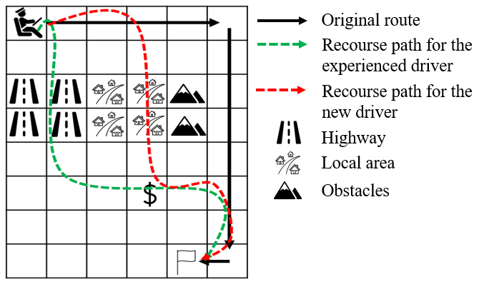
Figure 1: The original route $\tau_{0}$ (the driver didn’t collect reward), the recourse paths for the experienced driver $\tau_{\text{exp}}$ and the recourse path for the new driver $\tau_{\text{new}}$.

We simulate two types of taxi drivers as two agents. Driver $A_{\text{exp}}$ is an experienced driver who’s comfortable driving on the highway, and driver $A_{\text{new}}$ is a newbie driver who prefers to avoid the highway and take local roads instead. We simulate these two drivers by designing different reward functions. Agent $A_{\text{exp}}$ is trained by setting higher rewards for the highway area and lower rewards for the local area and vice versa for training agent $A_{\text{new}}$. Then the policy functions for the agents are provided as input to PPR.

We then run Algorithm 1 to generate personalized better routes for each agent. We set $\lambda_{\text{pe}}=0.1,\lambda_{\text{sim}}=0.1$ in Algorithm 1 (see the supplementary material for a sensitivity analysis of $\lambda_{\text{pe}}$ and $\lambda_{\text{sim}}$.) We show an example in Figure 1. As we can see, the recommended path $\tau_{\text{exp}}$ that is personalized for the experienced driver passes through the highway area because it follows the experienced driver policy. Likewise, the recommended route $\tau_{\text{new}}$ for the newbie driver takes a local road, also following his preferences reflected by the policy function. In this example, those new routes are the recourse paths of the original route, as they respect the driver’s driving behavior and facilitate a better outcome for the taxi while being similar to the old route from the starting point to the destination. Please refer to the supplementary material for all 10 routes and recourse paths.

We compare PPR with BL1 (BL2 is not applicable). Figure 2(a) shows the violin plots of the three scores from PPR and BL1. Since BL1 works by changing $k$ actions at most, the similarity scores have a lower variance than PPR. However, both personalization and goal scores of PPR are significantly higher, especially the personalization score, which is not considered by BL1.

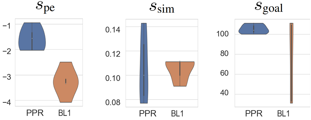
(a) $s_{\text{pe}}$, $s_{\text{sim}}$ ,$s_{\text{goal}}$ for PPR and BL1 trained on grid-world

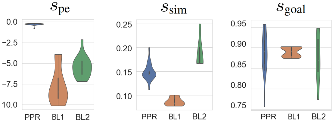
(b) $s_{\text{pe}}$, $s_{\text{sim}}$ ,$s_{\text{goal}}$ for PPR, BL1 and BL2 trained on temperature sequences (see the supplementary material for more details for this experiment).

Figure 2: Personalization score $s_{\text{pe}}$, similarity score $s_{\text{sim}}$, and goal score $s_{\text{goal}}$ of PPR and baselines BL1 and BL2.

5.2 Mario Environment

The second setting is the Mario environment provided by the OpenAI gym. This environment replicates the classic “Super Mario Bros” game, where the player-controlled character, Mario, navigates through diverse levels filled with obstacles, enemies, and power-ups and the primary objective is to reach the end of each level. We work with level 1 and for simplicity, in our experiments, Mario can only take two actions for each state: move right or jump right. A player can complete a level through various routes, which results in either winning by reaching the flag or losing by falling off a cliff or touching an enemy (e.g., a Goombas).

In this environment, we simulate two types of players with different playing styles. The first player likes to collect coins when playing the game and we call him a coin seeker. To simulate a coin seeker, we provide an additional 100 whenever a coin is collected. The agent will then try to collect as many coins as possible by jumping at appropriate places. To contrast with the coin seeker, we simulate a different player who would avoid getting coins by giving a -100 reward whenever a coin is collected. We call the player coin dodger. The goal of simulating the two agents with the opposite behavior is to evaluate how that behavior is reflected in the recourse path.

Then we construct an original route $\tau_{0}$ where Mario keeps moving right until getting killed by running into a goomba. The original route is generated by always choosing the action of “go right”, thus the route is featured by Mario walking in a straight line on the ground.

Then we generate a recourse path for the coin seeker. We show a segment in Figure 3 for demonstration. In the recourse path, the player successfully jumps over the Goombas to avoid dying and also collects two coins, one before Goombas and one after. We contrast this path with a recourse path generated for a coin dodger, also shown in Figure 3. As expected, the coin dodger did not hit any coins on the segment.

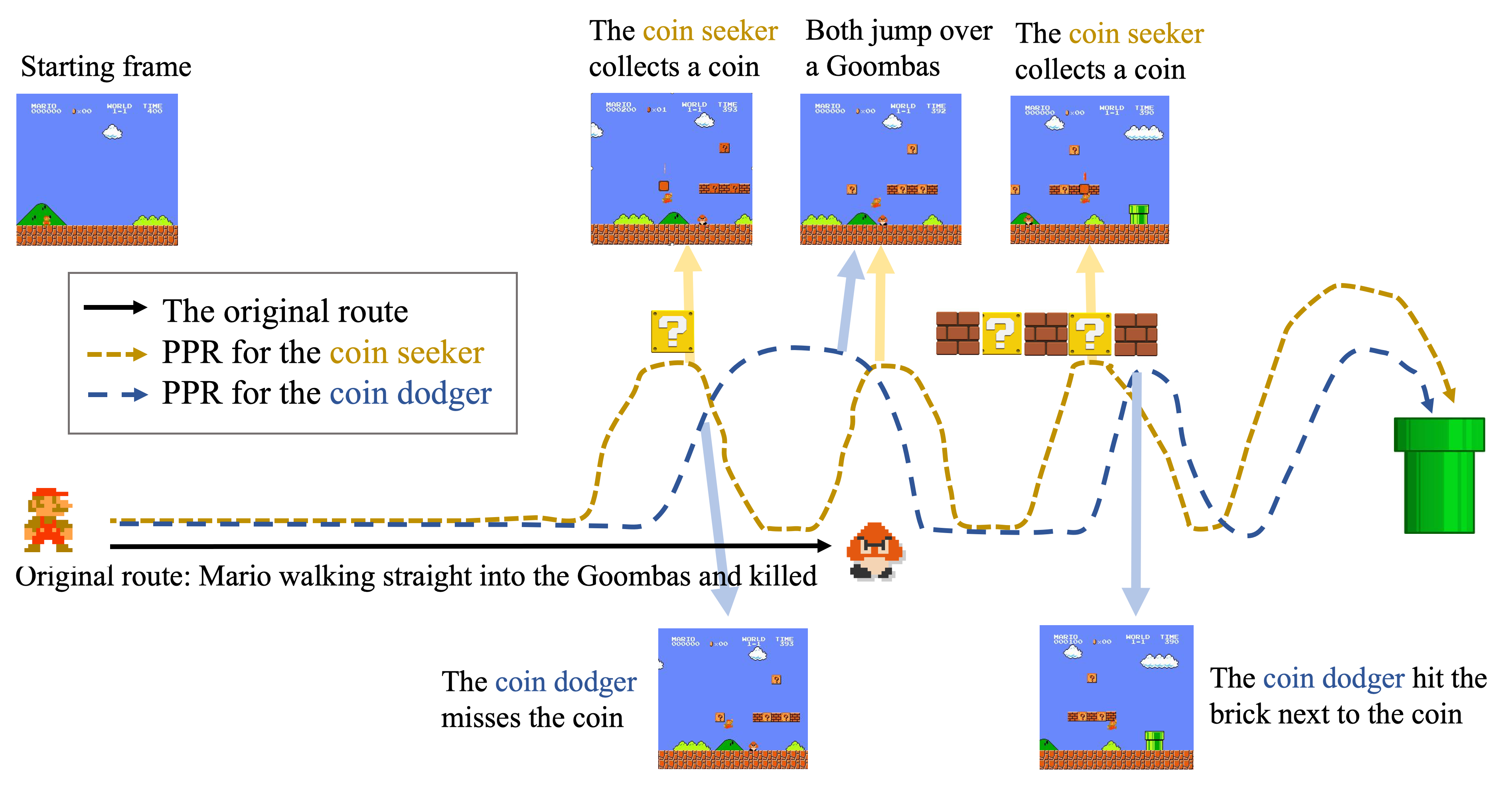
Figure 3: An illustration of one segment of level one of PPR generated for the coin seeker and coin dodger.

To quantitatively assess the extent to which the recourse path aligns with the preferences of the corresponding agent, we calculate the Kullback-Leibler (KL) divergence between the recoursed and original policy, shown in Table 1. To contrast with this “personalized” path, we also compare the policy of the PPR for the coin seeker with that of the coin dodger. In this case, while the generated path recourses the original route, it is not personalized to the coin dodger, thus significantly increasing the KL divergence from 0.342 to 1.049. We do the same for the coin seeker, comparing its policy function with the PPR generated for the coin dodger, and obtain a larger KL divergence of 0.554, up from 0.318 if it was personalized for him.

Table 1: The KL-divergence between agents’ policy functions and the PPR

	Coin Seeker	Coin Dodger
PPR for Coin Seeker	0.318	1.049
PPR for Coin Dodger	0.554	0.342

Note that baseline BL1 does not work for this experiment because it has to iterate through all the states of the environment, and the complexity of Mario environment is too high for BL1. BL2 is not applicable for reinforcement learning.

5.3 PPR for Text Data

In this application, we apply the method to generate recourse sequences for text. The goal is to change the sentiment of an original text (goal) while making as small changes as possible (similarity) and tailoring it to a specific writing style that represents a specific agent (personalization).

In this experiment, we train two language models as agents, an agent that represents the style of J.K. Rowling, trained from the 7 Harry Potter books, and another on the Bible corpus. We employ the transformer to train our language models, which assigns probabilities for the likelihood of a given word or sequence of words following a given sequence of words. To evaluate the sentiment, we use a pre-trained sentiment analysis model, such as NLTK’s sentiment library. This model returns a probability indicating the level of positive sentiment in the text. We use this sentiment score as the goal reward. It is worth noting that, PPR can directly work with an off-the-shelf language model and an evaluator (e.g., sentiment classifier), without accessing the training data, while many counterfactual explanation methods do need the training data to generate explanations.

To compare the recourse texts, we tune the hyperparameters by fixing $\lambda_{\text{pe}}$ to 1 and varying $\lambda_{\text{sim}}$. Table 1 illustrates a few recourse texts generated from various original texts with different personalization policies and $\lambda_{\text{sim}}$ values. As shown in Table 1, the generated recourse sequences are personalized towards the training corpus and exhibit positive sentiment. The degree of similarity between the recourse text and the original text is controlled by the value of $\lambda_{\text{sim}}$. Higher values of $\lambda_{\text{sim}}$ result in recourse texts that are more similar to the original text, while lower values lead to more flexible recourse texts that still maintain a positive sentiment. See the supplementary material for more results.

Please note that neither BL1 nor BL2 can be applied to this application. BL1 faces practical challenges because of its high computational complexity of $\mathcal{O}(n^{2}mTk)$ ($n,m,T,k$ are the number of states, the number of actions, sequence length and the number of actions changed, respectively). For text data, both states and action space are extremely large, making BL1 computationally infeasible and creating a timeout error. BL2 is also not applicable due to the unavailability of a labeled text dataset, while PPR can directly work with a trained sentiment classifier.

Table 2: Examples of text recourse with different writing styles and $\lambda_{\text{sim}}$.

Original text: She was sad
$\mathcal{P}_{A}$ trained from Harry Potter corpus: • $\lambda_{\text{sim}}=10$: She was very happy. • $\lambda_{\text{sim}}=0.1$: She giggled maliciously. $\mathcal{P}_{A}$ trained from Bible corpus: • $\lambda_{\text{sim}}=10$: She was exceedingly beautiful. • $\lambda_{\text{sim}}=0.1$: She shall glorify God and honor and she shall be known.
Original text: The cup was empty.
$\mathcal{P}_{A}$ trained from Harry Potter corpus: • $\lambda_{\text{sim}}=10$: The cup was very strong. • $\lambda_{\text{sim}}=0.1$: The cup and a strong love potion again. $\mathcal{P}_{A}$ trained from Bible corpus: • $\lambda_{\text{sim}}=10$: The cup was altogether lovely. • $\lambda_{\text{sim}}=0.1$: The cup is of the Lord, thy God with a blessing.
Original text: The book on the table is boring.
$\mathcal{P}_{A}$ trained from Harry Potter corpus: • $\lambda_{\text{sim}}=10$: The book on the wall and the other hand were completely invisible. • $\lambda_{\text{sim}}=0.1$: The book of interesting facts and Harry had a very enjoyable morning. $\mathcal{P}_{A}$ trained from Bible corpus: • $\lambda_{\text{sim}}=10$: The book of Jashar, thy glory, which is exalted at the right hand of God. • $\lambda_{\text{sim}}=0.1$: The book of Moses blessed the Lord and the God of Israel.

5.4 Other Experiments

We include more experiments in the supplementary material.

Extension to recourse of supervised models

As discussed in Section 4.3, PPR can also be applied to supervised learning settings. We use PPR to generate recourse sequences for yearly temperature patterns from a dataset with 200 years of yearly temperatures for Rome in Italy and Columbia in South Carolina, USA. In this experiment, we want to recourse the temperature sequences from one city to the other while ensuring the generated sequence is similar to the original temperate (similarity) and still follows the pattern and style of the temperature patterns in the data (personalization). Results are shown in Figure 2 (b).

For example, to recourse a Rome temperature sequence to Columbia (goal), we begin by training a generator model on all temperature data, which acts as the personalized policy for our algorithm. Next, we train a classifier on our dataset, and the classification probability score serves as the goal reward, which has a higher score indicating a higher chance that the temperature sequence belongs to Columbia. We use standard LSTM architecture for both the generator model and the classifier. Finally, we execute Algorithm 1 to generate recourse sequences. Figure 4 presents the given original temperature sequences and the corresponding recourse sequences generated from PPR. We also show the sequences generated by BL1 and BL2 for comparison.

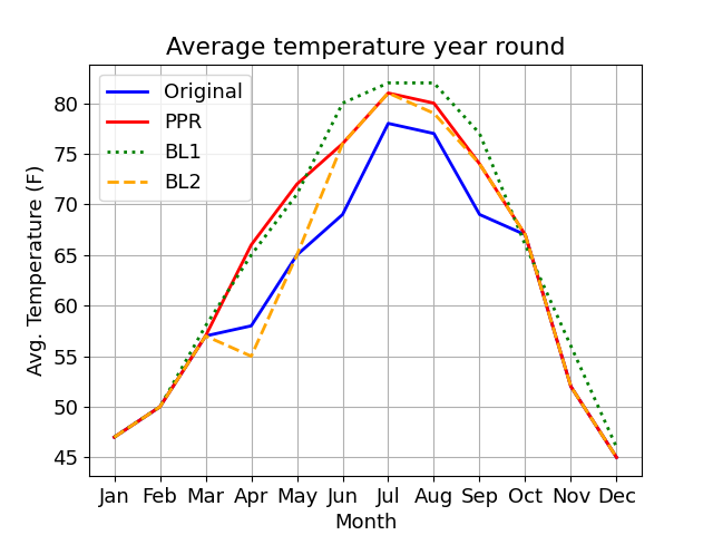
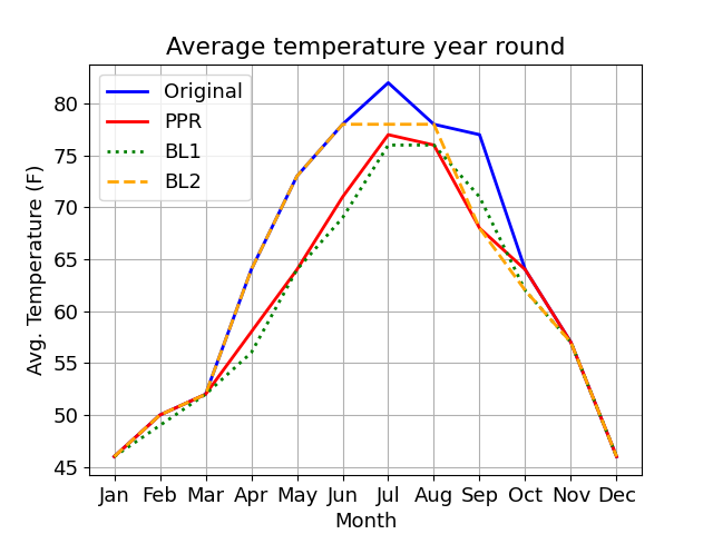
(a) recourse from Rome to Columbia

(b) recourse from Columbia to Rome

Figure 4: Examples of recourse temperate generated by different methods

Our recourse sequences show a high degree of similarity to the original temperature sequences. For example, in Figure 4(a), the recourse sequences accurately reflect the temperature pattern in Columbia while closely resembling the temperature pattern of Rome during fall and winter months (from October to March). The recourse sequences reveal that the main differences between the two cities’ temperature patterns lie in the summer months.

Figure 2(b) compares $s_{\text{pe}},s_{\text{sim}}$ and $s_{\text{goal}}$ of PPR with BL1 and BL2. Overall, PPR achieves significantly higher $s_{\text{pe}}$ scores while maintaining $s_{\text{goal}}$ scores. Having low $s_{\text{pe}}$ indicates that some of the sequences generated by BL1 and BL2 deviate from the data distribution. For instance, BL2 shows April is colder than March in Figure 4(a), and all three summer months have the same temperatures in Figure 4(b) – these are inconsistent with the patterns in training data, indicating the generated sequence is out of distribution. BL1 has a lower similarity to the original temperature - the recourse sequence deviates from the original sequence more than necessary. As shown in Figure 4 (a) and (b), PPR only needs to change the summer temperatures, leaving other months the same, while BL1 changes the temperature of almost every month, though smaller changes in winter. In addition, BL1 has high variance in terms of the personalization score, as it exhaustively searches all possible states in the dataset.

Influence of $\lambda_{\text{pe}}$ and $\lambda_{\text{sim}}$

We also investigate the influence of $\lambda_{\text{pe}}$ and $\lambda_{\text{sim}}$ from equation (6) on recourse path quality. For this type of experiment, we set different values for $\lambda_{\text{pe}}$, $\lambda_{\text{sim}}$, and report the average $s_{\text{pe}},s_{\text{sim}}$ and $s_{\text{goal}}$ of the recourse paths in the generated recourse path set. The details of the experiment setup and results can be found in the supplementary material. In general, the higher values of $\lambda_{\text{pe}}$ and $\lambda_{\text{sim}}$ are, the higher $s_{\text{pe}}$ and $s_{\text{sim}}$ obtained. When both of these values are low, the recourse paths tend to have higher goal reward $s_{\text{goal}}$.

6 Conclusion

We introduced Personalized Path Recourse (PPR), which generates personalized paths of actions that achieve a certain goal (e.g., a better outcome) for an agent. Our approach extends the existing literature on counterfactual explanations and generates entire personalized paths of actions, rather than just explaining why an action is chosen over others. Existing baselines either do not work for applications with large state and action space, or can only be applied to supervised learning. PPR, on the other hand, can be applied to a broader set of applications.

Limitations

First, the current PPR approach only applies to discrete states or sequences. Therefore, future work could explore the application of PPR to more complex decision-making scenarios that possibly involve continuous states and diverse data modalities. Another limitation is the availability of an agent’s policy function in order to be personalized, which needs to be either provided or trained from sufficient data observed from the agent. Thus, future work can focus on how to efficiently learn agent’s policy function from limited data.

Impact Statements

This paper presents work whose goal is to advance the field of Machine Learning. There are many potential societal consequences of our work, none of which we feel must be specifically highlighted here.

Appendix A Experiment design

All the codes for the experiments are uploaded in the supplementary materials with the instruction .txt file. They are implemented in Python 3.9 and Pytorch 1.13. All the models are trained on GPU NVIDIA GeForce GTX 1660 Ti. The training process uses AdamOptimizer https://pytorch.org/docs/stable/generated/torch.optim.Adam.html.

A.1 Grid-world

Experiment set-up

In this experiment, we create a 8x6 array and set $b=200,k=1,\lambda=0.99,c_{exp}=1,\lambda_{\text{pe}}=0.1,\lambda_{\text{sim}}=0.1,\text{decay}\>\epsilon=0.001,C=1$ to run the Algorithm 1. The learning rate was $1e-3$ We select 10 random original routes and generate 10 corresponding recourse paths. We report one example in Figure 1 in the main paper.

Original and recoursed paths

In addition to the example in the main paper, the other 8 original routes and the corresponding recourse paths trained on experienced driver policy are shown in Figure 5. We use those results to generate the plots in Figure 2(a) in the main paper.

(a)

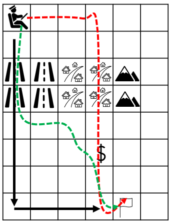
(b)

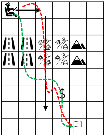
(c)

(d)

(e)

(f)

(g)

(h)

Figure 5: Other random original routes and the corresponding recourse paths, in addition to Figure 1.

Sensitivity Analysis

We conduct sensitivity analysis using the same 10 original routes but with different values of $\lambda_{\text{pe}},\lambda_{\text{sim}}$.We report the heatmaps of the average scores of $s_{\text{pe}},s_{\text{sim}},s_{\text{goal}}$ in Figure 6. In general, the higher values of $\lambda_{\text{pe}}$ and $\lambda_{\text{sim}}$ are, the higher $s_{\text{pe}}$ and $s_{\text{sim}}$ we can get. When both of these values are low, such as 0.01, the PPRs tend to have higher goal reward $s_{\text{goal}}$.

(a) Personalization $s_{\text{pe}}$

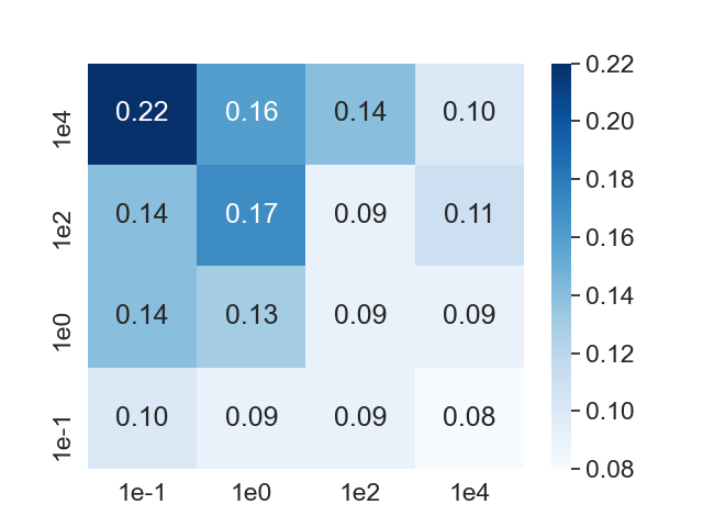
(b) Similarity $s_{\text{sim}}$

(c) Goal score $s_{\text{goal}}$

Figure 6: Personalization, similarity and goal score $s_{\text{pe}},s_{\text{sim}},s_{\text{goal}}$ for the grid-world experiment. The x-axis indicates different values of $\lambda_{\text{sim}}$ and the y-axis shows different values of $\lambda_{\text{pe}}$.

Baselines

As a reminder, BL2 is not applicable because it is designed only for classification tasks in supervised learning settings. We are comparing our method PPR to BL1 in this application. We implement BL1 by exhaustively searching all possible states and actions of the environment and recording all the valid paths (the ones that do not fall off the grid nor pass through the obstacles). The path with the maximum goal reward is reported. $k$ is set empirically for BL1. Note that BL1 aims to find a recourse path that has $k$ different actions from the original path while maintaining the same length. Therefore, when the original path is too short, recourse paths generated from BL1 may not reach the final destination. This is one of the reasons why its goal reward is low in some cases.

A.2 Mario Game

In this paper, we implement PPR based on the Mario Reinforcement Learning tutorial from https://pytorch.org/tutorials/intermediate/mario_rl_tutorial.html by Yuansong Feng, Suraj Subramanian, Howard Wang, and Steven Guo. The tutorial gives instructions on how to train Mario agent to play itself by using Double Deep Q-Networks) using PyTorch. In this tutorial, Mario’s action space is limited to only two actions: Walk Right or Jump Right. The real state is created by stacking up 3 consecutive game frames, which are also reduced to grayscale. For all the experiments, we train Mario on the first stage/mission only.

The Mario environment, powered by Open AI gym gym-super-mario-bros, provided the info variable to help users collect the information from the environment such as how many coins Mario collected, how many scores Mario has had, the (x,y) coordinate of the agent’s current position, how many lives remaining, etc. By default, the environment reward considers three factors: the difference in agent x values between states, the difference in the game clock between frames, and a death penalty that penalizes the agent for dying in a state. The environment reward is capped to a [-15,15] range. In our experiments, this reward is used as the goal reward. To train a policy to encourage the agent to collect coins, we alter the environment by giving an extra +100 reward whenever Mario collects a coin. Similarly, a reward of -100 will be taken from the agent to discourage it from collecting coins.

To implement PPR, we set $\lambda_{sim}=100$ and $\lambda_{pe}=10$. All the policies are trained with at least 50,000 episodes. Figure 7 shows the probability distribution of taking action ”Jump Right” for all policies: coin seeker, coin dodger, and their PPR policies for the first 460 steps (x-coordinate).

(a) Coin seeker

(b) PPR for coin seeker

(c) Coin dodger

(d) PPR for coin dodger

Figure 7: Probability distributions of action ”Jump Right” at each position. ’O’ indicates where Mario takes “Jump” actions and ’X’ indicates where Mario takes ’Walk’ (“no jump”) actions.

A.3 Temperature

Dataset In this experiment, we use the temperature dataset from Kaggle https://www.kaggle.com/datasets/sudalairajkumar/daily-temperature-of-major-cities, which contains daily average temperature values recorded in major cities of the world. We choose 2 cities Rome from Italy and Columbia from North Carolina, USA. For each city, we compute the average monthly temperature for each year from 1995 to 2020. This results in 25 temperature sequences with lengths of 12 for each city. We also apply data augmentation by randomly adding or subtracting randomly 1-2 degrees from each month, while maintaining the order pattern of each sequence. The label for each sequence is the city (either Rome or Columbia). We choose 200 temperature sequences for the training dataset and 20 sequences for the test dataset (10 temperature sequences for Rome and 10 temperature sequences for Columbia).

Experiment set-up

To run Algorithm 1 in the main paper, we set $b=500,k=1,\lambda=0.99,c_{exp}=1,\lambda_{\text{pe}}=0.1,\lambda_{\text{sim}}=10,\text{decay}\>\epsilon=0.001,C=1$. The learning rate value is $1e-3$. We train the generator and the classifier using the standard LSTM architecture.

Original sequences and recoursed sequences

Figure 8 and 9 show the 20 original temperature sequences from the test set and the corresponding recourse paths generated.

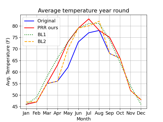
(a)

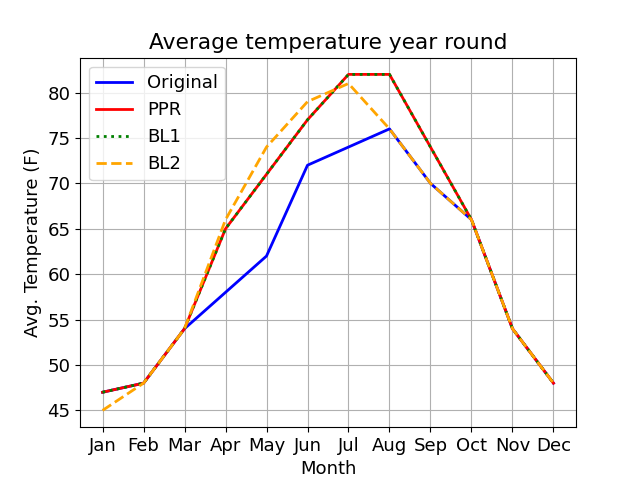
(b)

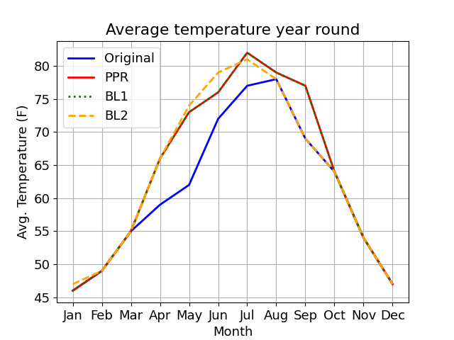
(c)

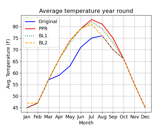
(d)

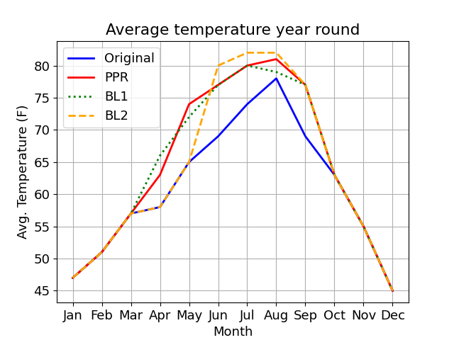
(e)

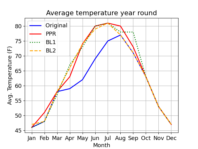
(f)

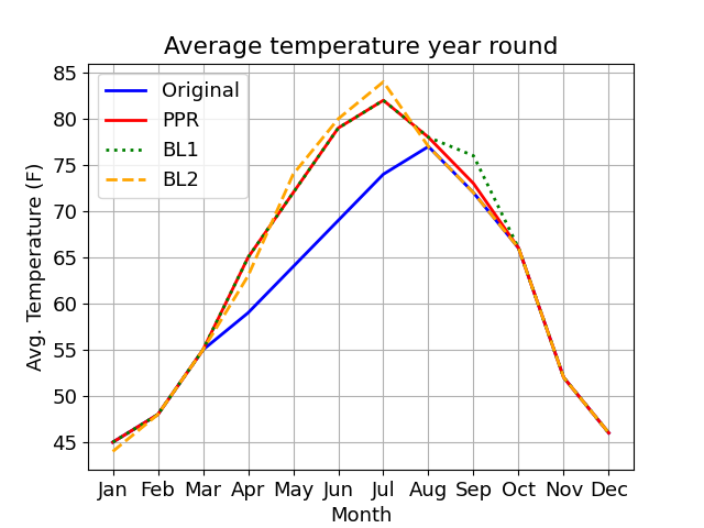
(g)

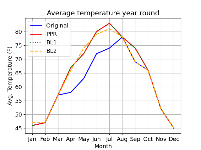
(h)

Figure 8: Original temperatures (from Rome) from the test set and the corresponding recourse paths from PPR, BL1, BL2.

(a)

(b)

(c)

(d)

(e)

(f)

(g)

(h)

(i)

Figure 9: Original temperatures (from Columbia) from the test set and the corresponding recourse paths from PPR, BL1, BL2.

Sensitivity Analysis

We also conduct sensitivity analysis with values for $\lambda_{\text{pe}},\lambda_{\text{sim}}$. Figure 10 shows the heatmaps of the average score of $s_{\text{pe}},s_{\text{sim}},s_{\text{goal}}$ based on different values of $\lambda_{pe},\lambda_{sim}$. Similar to the grid-world experiment, in general, the larger $\lambda_{\text{pe}}$ and $\lambda_{\text{sim}}$, the higher $s_{\text{pe}}$ and $s_{\text{sim}}$ are. When both of these values are low, such as 0.01, the PPRs tend to have higher goal reward $s_{\text{goal}}$.

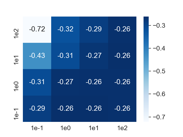
(a) Personalization $s_{\text{pe}}$

(b) Similarity $s_{\text{sim}}$

(c) Goal score $s_{\text{goal}}$

Figure 10: Personalization, similarity and goal score $s_{\text{pe}},s_{\text{sim}},s_{\text{goal}}$ for the temperature experiment. The x-axis indicates different values of $\lambda_{\text{sim}}$ and y-axis shows different values of $\lambda_{\text{pe}}$.

Baselines

For this application, a naive implementation of BL1 is still not applicable due to its high computational complexity. For instance, if we allow the temperature ranges from 1 to 100, we will have $|\mathcal{A}|=100$ and $|\mathcal{S}|=100^{12}$, which are too large to fit in the memory for the dynamic programming method. Therefore, we modified BL1 by only considering the available states and actions in the dataset. On the other hand, BL2 aims to find the recourse sequence by first searching for the best candidate sequence with a different label from the original sequence. Then, it replaces a subsequence in the original sequence with another subsequence extracted from this candidate. Therefore, sometimes the generated recourse sequences contain some abnormal patterns. For example, in figure 9(a), we can observe April’s temperature is lower than March’s in the recourse sequence generated by BL2.

A.4 Text generation

Dataset

In this experiment, we employ Transformer to train two language models: one on all 7 Harry Potter books by J.K. Rowling and another on the Bible corpus. The link to the Harry Potter corpus can be found at https://www.kaggle.com/code/balabaskar/harry-potter-text-analysis-starter-notebook while the Bible text corpus is downloaded from https://openbible.com/textfiles/asv.txt. We do text preprocessing before training: for the Harry Potter corpus, we merge all the books into one corpus. For the Bible corpus, we remove all ”Genesis” terms from the text files because of their redundancy. We also convert all the text into lower-case before training.

Experiment set-up

The language models are trained with GPU NVIDIA GeForce GTX 1660 Ti. accelerator in three days. Our transformer has an embedding dimension size of 200, the dimension of the feedforward network model is 200, 2 transformer encoding layers, and 2 multi-head attention. We also set the dropout rate to 0.2. We set $b=500,k=1,\lambda=0.99,c_{exp}=0.01,\text{decay}\>\epsilon=0.001,C=1$. In this experiment, we modify values of $\lambda_{pe},\lambda_{sim}$ before generating the recourse text.

Examples of original texts and recoursed texts

In addition to Table 2, Table 3 shows examples of the recourse texts that flip the sentiment labels from positive to negative.

Table 3: More examples of text recourse with different writing styles that flip the sentiment from positive to negative.

Original text and text sampled from $\mathcal{P}_{A}$ trained on Harry Potter and Bible corpus (with the corresponding $\lambda_{\text{sim}}$ value)
Original text: I am in love.
$\mathcal{P}_{A}$ trained from Harry Potter corpus: • $\lambda_{\text{sim}}=10$: I am sorry, it is my fault. • $\lambda_{\text{sim}}=0.1$: ”I didn’t. Feel so stupid”, said Ron. $\mathcal{P}_{A}$ trained from Bible corpus: • $\lambda_{\text{sim}}=10:$ I am in distress. • $\lambda_{\text{sim}}=0.1:$ I have seen my face and my sorrow is stirred.
Original text: The world is beautiful.
$\mathcal{P}_{A}$ trained from Harry Potter corpus: • $\lambda_{\text{sim}}=10$: The world is very nosy. • $\lambda_{\text{sim}}=0.1$: The world and the cup is not strong. $\mathcal{P}_{A}$ trained from Bible corpus: • $\lambda_{\text{sim}}=10$: The world is fallen. • $\lambda_{\text{sim}}=0.1$: The world were crucified with him but saved us alive.
Original text: The magicians enjoy the magic.
$\mathcal{P}_{A}$ trained from Harry Potter corpus: • $\lambda_{\text{sim}}=10$: The magician had not committed this crime. • $\lambda_{\text{sim}}=0.1$: The magic was expelled at Hogwarts. $\mathcal{P}_{A}$ trained from Bible corpus: • $\lambda_{\text{sim}}=10$: The magicians of Egypt as an adversary and did as an evil man. • $\lambda_{\text{sim}}=0.1$: The magicians of Egypt, but behold, they will bring their evil against their houses.

Baselines

Remind that neither BL1 nor BL2 can be applied to this application. BL1 faces practical challenges because of its high computational complexity of $\mathcal{O}(n^{2}mTk)$ ($n,m,T,k$ are the number of states, the number of actions, sequence length and the number of actions changed, respectively). For text data, both states and action space are extremely large, making BL1 computationally infeasible and creating a timeout error. BL2 is also not applicable due to the unavailability of a labeled text dataset, while PPR can directly work with a trained sentiment classifier.

Appendix B Model Design Choices

B.1 Levenshtein distance formula

The Levenshtein distance between two sequences $\tau_{0}=<\mathbf{s}^{\tau_{0}}_{1},\mathbf{s}^{\tau_{0}}_{2},...,\mathbf{s}^{\tau_{0}}_{i}>$ and $\tau_{r}=<\mathbf{s}^{\tau_{r}}_{1},\mathbf{s}^{\tau_{r}}_{2},...,\mathbf{s}^{\tau_{r}}_{j}>$ with length $i$ and $j$ respectively is defined as:

$$d_{ij}(\tau_{0},\tau_{r})=\left\{\begin{array}[]{ll}d_{i-1,j-1}&\mathrm{if}\>\>{\mathbf{s}_{i}^{\tau_{0}}}\par=\mathbf{s}_{j}^{\tau_{r}}\\ \mathrm{min}(d_{i-1,j}+w_{del}(\mathbf{s}_{i}^{\tau_{0}}),\\ d_{i,j-1}+w_{ins}(\mathbf{s}^{\tau_{r}}_{j}),\\ d_{i-1,j-1}+w_{sub}(\mathbf{s}_{i}^{\tau_{0}},\mathbf{s}^{\tau_{r}}_{j}))&\mathrm{if}\>\>\mathbf{s}_{i}^{\tau_{0}}\neq\mathbf{s}_{j}^{\tau_{r}}\end{array}\right.$$

Here $w_{del}(\cdot),w_{ins}(\cdot)$ and $w_{sub}(\cdot,\cdot)$ are the functions returning the weighting scores of deletion, insertion, and substitution operation, respectively. In this paper, we set all those values to 1.

B.2 Personalization reward design

In this section, we explain the design of Equation (4) of the $h(.)$ function in the main paper. As a reminder, we design a link function $h(\cdot)$ that needs to satisfy the conditions as follows:

1. $h(p)$ increases monotonically with probability $p$.

2. $h(p)>0$ when $p>\frac{1}{|\mathcal{A}|}$, $h(p)=0$ when $p=\frac{1}{|\mathcal{A}|}$, and $h(p)<0$ when $p<\frac{1}{|\mathcal{A}|}$.

3. When $p$ is close to 1, $h(p)$ is a large positive number and when $p$ is close to 0, $h(p)$ is a large negative number.

In addition, we would like to penalize $h(.)$ when it reaches a too high or too low value by adding $\log()$ factor. Then $h(.)$ has the form:

$$h(p)=\log(\frac{f(p)}{g(p)})$$ (9)

$h(p)$ must increase monotonically with probability $p$. For simplicity, we assume $f(p),g(p)$ are linear functions, so we can write $h(p)$ as:

$$h(p)=\log(\frac{A_{1}p+B_{1}}{A_{2}p+B_{2}})$$ (10)

First, assuming $\frac{1}{|\mathcal{A}|}<p<1$, when $p$ is close to 1, we want $h(p)$ to have high positive number. This can be achieved by set $g(p)=A_{2}p+B_{2}=0$ when $p=1$, which is equivalent to $A_{2}=-B_{2}$. Plus the condition $\frac{1}{|\mathcal{A}|}<p<1$, then we can choose $B_{2}=1$ and $A_{2}=-1$. The final form of $g(p)$ is:

$$g(p)=1-p$$ (11)

Furthermore, we want $h(p)$ to be 0 when $p=\frac{1}{|\mathcal{A}|}$. From (8), this is equivalent to $\frac{f(p)}{g(p)}=1$ or $f(p)=g(p)$ when $p=1/{|\mathcal{A}|}$. Replace with (10), we have:

$$A_{1}p+B_{1}=1-p\>\>\text{when}\>\>p=1/|\mathcal{A}|\Longleftrightarrow\frac{A_{1}}{|\mathcal{A}|}+B_{1}=1-\frac{1}{|\mathcal{A}|}\Longleftrightarrow B_{1}=1-\frac{1+A_{1}}{|\mathcal{A}|}$$ (12)

If we choose $A_{1}=1$ then $B_{1}=1-\frac{2}{|\mathcal{A}|}$.

So when $\frac{1}{|\mathcal{A}|}<p<1$, the final form of $h(.)$ is:

$$h(p)=\log(\frac{p-\frac{2}{|\mathcal{A}|}+1}{1-p})$$ (13)

Next, assuming $0<p<\frac{1}{|\mathcal{A}|}$. With similar reasoning, we want $h(p)$ to be a very low negative value when $p=0$. This is a natural property of $\log(.)$ function, so $h(.)$ can have the form:

$$h(p)=\log(A\>p)$$ (14)

We want $h(p)=0$ when $p=1/|\mathcal{A}|$, this is equivalent to $Ap=1$ when $p=1/|\mathcal{A}|$, or $\frac{A}{|\mathcal{A}|}=1\Longleftrightarrow A=|\mathcal{A}|$. Then, $h(p)$ has the form:

$$h(p)=\log(|\mathcal{A}|p)$$ (15)

So, to sum up, the final form of $h(p)$ defined on domain [0,1] is:

$$h(p)=\begin{cases}\log(\frac{p-\frac{2}{|\mathcal{A}|}+1}{1-p})&\text{if $p>=\frac{1}{\mathcal{|A|}}$,}\\ \log(|\mathcal{A}|\cdot p)&\text{otherwise}.\end{cases}$$ (16)

which is Equation (4) in the main paper. Figure 3 illustrates the graph of $h()$ function.

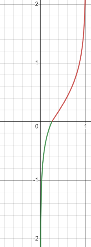
Figure 11: Visualization of $h()$ function

References

- Andrychowicz et al. (2017) Andrychowicz, M., Wolski, F., Ray, A., Schneider, J., Fong, R., Welinder, P., McGrew, B., Tobin, J., Pieter Abbeel, O., and Zaremba, W. Hindsight experience replay. Advances in neural information processing systems, 30, 2017.
- Ates et al. (2021) Ates, E., Aksar, B., Leung, V. J., and Coskun, A. K. Counterfactual explanations for multivariate time series. In 2021 International Conference on Applied Artificial Intelligence (ICAPAI), pp. 1–8. IEEE, 2021.
- Dandl et al. (2020) Dandl, S., Molnar, C., Binder, M., and Bischl, B. Multi-objective counterfactual explanations. In International Conference on Parallel Problem Solving from Nature, pp. 448–469. Springer, 2020.
- (4) De Toni, G., Viappiani, P., Teso, S., Lepri, B., and Passerini, A. Personalized algorithmic recourse with preference elicitation.
- De Toni et al. (2023) De Toni, G., Lepri, B., and Passerini, A. Synthesizing explainable counterfactual policies for algorithmic recourse with program synthesis. Machine Learning, 112(4):1389–1409, 2023.
- Delaney et al. (2021) Delaney, E., Greene, D., and Keane, M. T. Instance-based counterfactual explanations for time series classification. In International Conference on Case-Based Reasoning, pp. 32–47. Springer, 2021.
- Frost et al. (2022) Frost, J., Watkins, O., Weiner, E., Abbeel, P., Darrell, T., Plummer, B., and Saenko, K. Explaining reinforcement learning policies through counterfactual trajectories. arXiv preprint arXiv:2201.12462, 2022.
- Gajcin & Dusparic (2022) Gajcin, J. and Dusparic, I. Counterfactual explanations for reinforcement learning. arXiv preprint arXiv:2210.11846, 2022.
- Gajcin & Dusparic (2023) Gajcin, J. and Dusparic, I. Raccer: Towards reachable and certain counterfactual explanations for reinforcement learning. arXiv preprint arXiv:2303.04475, 2023.
- Goyal et al. (2019) Goyal, Y., Wu, Z., Ernst, J., Batra, D., Parikh, D., and Lee, S. Counterfactual visual explanations. In International Conference on Machine Learning, pp. 2376–2384. PMLR, 2019.
- Harris et al. (2022) Harris, K., Chen, V., Kim, J., Talwalkar, A., Heidari, H., and Wu, S. Z. Bayesian persuasion for algorithmic recourse. Advances in Neural Information Processing Systems, 35:11131–11144, 2022.
- Hsieh et al. (2021) Hsieh, C., Moreira, C., and Ouyang, C. Dice4el: interpreting process predictions using a milestone-aware counterfactual approach. In 2021 3rd International Conference on Process Mining (ICPM), pp. 88–95. IEEE, 2021.
- Joshi et al. (2019) Joshi, S., Koyejo, O., Vijitbenjaronk, W., Kim, B., and Ghosh, J. Towards realistic individual recourse and actionable explanations in black-box decision making systems. arXiv preprint arXiv:1907.09615, 2019.
- Karimi et al. (2020) Karimi, A.-H., Barthe, G., Schölkopf, B., and Valera, I. A survey of algorithmic recourse: definitions, formulations, solutions, and prospects. arXiv preprint arXiv:2010.04050, 2020.
- Karimi et al. (2021) Karimi, A.-H., Schölkopf, B., and Valera, I. Algorithmic recourse: from counterfactual explanations to interventions. In Proceedings of the 2021 ACM conference on fairness, accountability, and transparency, pp. 353–362, 2021.
- Karlsson et al. (2020) Karlsson, I., Rebane, J., Papapetrou, P., and Gionis, A. Locally and globally explainable time series tweaking. Knowledge and Information Systems, 62(5):1671–1700, 2020.
- Levenshtein et al. (1966) Levenshtein, V. I. et al. Binary codes capable of correcting deletions, insertions, and reversals. In Soviet physics doklady, volume 10, pp. 707–710. Soviet Union, 1966.
- Madumal et al. (2020) Madumal, P., Miller, T., Sonenberg, L., and Vetere, F. Explainable reinforcement learning through a causal lens. In Proceedings of the AAAI conference on artificial intelligence, volume 34, pp. 2493–2500, 2020.
- Olson et al. (2019) Olson, M. L., Neal, L., Li, F., and Wong, W.-K. Counterfactual states for atari agents via generative deep learning. arXiv preprint arXiv:1909.12969, 2019.
- Pawlowski et al. (2020) Pawlowski, N., Coelho de Castro, D., and Glocker, B. Deep structural causal models for tractable counterfactual inference. Advances in Neural Information Processing Systems, 33:857–869, 2020.
- Poyiadzi et al. (2020) Poyiadzi, R., Sokol, K., Santos-Rodriguez, R., De Bie, T., and Flach, P. Face: feasible and actionable counterfactual explanations. In Proceedings of the AAAI/ACM Conference on AI, Ethics, and Society, pp. 344–350, 2020.
- Puterman (2014) Puterman, M. L. Markov decision processes: discrete stochastic dynamic programming. John Wiley & Sons, 2014.
- Racanière et al. (2017) Racanière, S., Weber, T., Reichert, D., Buesing, L., Guez, A., Jimenez Rezende, D., Puigdomènech Badia, A., Vinyals, O., Heess, N., Li, Y., et al. Imagination-augmented agents for deep reinforcement learning. Advances in neural information processing systems, 30, 2017.
- Ross et al. (2021) Ross, A., Lakkaraju, H., and Bastani, O. Learning models for actionable recourse. Advances in Neural Information Processing Systems, 34:18734–18746, 2021.
- Schaul et al. (2015) Schaul, T., Quan, J., Antonoglou, I., and Silver, D. Prioritized experience replay. arXiv preprint arXiv:1511.05952, 2015.
- Sulem et al. (2022) Sulem, D., Donini, M., Zafar, M. B., Aubet, F.-X., Gasthaus, J., Januschowski, T., Das, S., Kenthapadi, K., and Archambeau, C. Diverse counterfactual explanations for anomaly detection in time series. arXiv preprint arXiv:2203.11103, 2022.
- Thiagarajan et al. (2021) Thiagarajan, J., Narayanaswamy, V. S., Rajan, D., Liang, J., Chaudhari, A., and Spanias, A. Designing counterfactual generators using deep model inversion. Advances in Neural Information Processing Systems, 34:16873–16884, 2021.
- Tsirtsis & Gomez Rodriguez (2020) Tsirtsis, S. and Gomez Rodriguez, M. Decisions, counterfactual explanations and strategic behavior. Advances in Neural Information Processing Systems, 33:16749–16760, 2020.
- Tsirtsis et al. (2021) Tsirtsis, S., De, A., and Rodriguez, M. Counterfactual explanations in sequential decision making under uncertainty. Advances in Neural Information Processing Systems, 34:30127–30139, 2021.
- Upadhyay et al. (2021) Upadhyay, S., Joshi, S., and Lakkaraju, H. Towards robust and reliable algorithmic recourse. Advances in Neural Information Processing Systems, 34:16926–16937, 2021.
- Ustun et al. (2019) Ustun, B., Spangher, A., and Liu, Y. Actionable recourse in linear classification. In Proceedings of the conference on fairness, accountability, and transparency, pp. 10–19, 2019.
- Van Looveren et al. (2021) Van Looveren, A., Klaise, J., Vacanti, G., and Cobb, O. Conditional generative models for counterfactual explanations. arXiv preprint arXiv:2101.10123, 2021.
- Verma et al. (2020) Verma, S., Boonsanong, V., Hoang, M., Hines, K. E., Dickerson, J. P., and Shah, C. Counterfactual explanations and algorithmic recourses for machine learning: A review. arXiv preprint arXiv:2010.10596, 2020.
- Verma et al. (2022) Verma, S., Hines, K., and Dickerson, J. P. Amortized generation of sequential algorithmic recourses for black-box models. In Proceedings of the AAAI Conference on Artificial Intelligence, volume 36, pp. 8512–8519, 2022.
- Wachter et al. (2017) Wachter, S., Mittelstadt, B., and Russell, C. Counterfactual explanations without opening the black box: Automated decisions and the gdpr. Harv. JL & Tech., 31:841, 2017.
- Wang et al. (2016) Wang, Z., Schaul, T., Hessel, M., Hasselt, H., Lanctot, M., and Freitas, N. Dueling network architectures for deep reinforcement learning. In International conference on machine learning, pp. 1995–2003. PMLR, 2016.
- Wang et al. (2021) Wang, Z., Samsten, I., Mochaourab, R., and Papapetrou, P. Learning time series counterfactuals via latent space representations. In Discovery Science: 24th International Conference, DS 2021, Halifax, NS, Canada, October 11–13, 2021, Proceedings 24, pp. 369–384. Springer, 2021.
- Yetukuri et al. (2022) Yetukuri, J., Hardy, I., and Liu, Y. Actionable recourse guided by user preference. 2022.
- Zahavy et al. (2021) Zahavy, T., O’Donoghue, B., Barreto, A., Mnih, V., Flennerhag, S., and Singh, S. Discovering diverse nearly optimal policies with successor features. arXiv preprint arXiv:2106.00669, 2021.