Stein-MAP: A Sequential Variational Inference Framework for Maximum A Posteriori Estimation

Abstract

State estimation poses substantial challenges in robotics, often involving encounters with multimodality in real-world scenarios. To address these challenges, it is essential to calculate Maximum a posteriori (MAP) sequences from joint probability distributions of latent states and observations over time. However, it generally involves a trade-off between approximation errors and computational complexity. In this article, we propose a new method for MAP sequence estimation called Stein-MAP, which effectively manages multimodality with fewer approximation errors while significantly reducing computational and memory burdens. Our key contribution lies in the introduction of a sequential variational inference framework designed to handle temporal dependencies among transition states within dynamical system models. The framework integrates Stein’s identity from probability theory and reproducing kernel Hilbert space (RKHS) theory, enabling computationally efficient MAP sequence estimation. As a MAP sequence estimator, Stein-MAP boasts a computational complexity of $O(N)$, where $N$ is the number of particles, in contrast to the $O(N^{2})$ complexity of the Viterbi algorithm. The proposed method is empirically validated through real-world experiments focused on range-only (wireless) localization. The results demonstrate a substantial enhancement in state estimation compared to existing methods. A remarkable feature of Stein-MAP is that it can attain improved state estimation with only $40$ to $50$ particles, as opposed to the $1000$ particles that the particle filter or its variants require.

I Introduction

State estimation is crucial for various fundamental tasks in autonomous systems, including localization, tracking, planning, and control. The Bayesian filter, widely used for state estimation, combines prior information with a likelihood function, following Bayes’ rule. Although Gaussian-based filters such as the Kalman filter (KF) [1], including variants such as the Extended Kalman Filter (EKF) [2] and the Unscented Kalman Filter (UKF) [3] for nonlinear systems, are prevalent, they have limitations in complex and multi-modal scenarios. To address these limitations, non-parametric approaches such as the particle filter (PF) [4] have been proposed, particularly for multimodal scenarios. However, handling high-dimensional systems with PF remains computationally challenging. In the field of robotics, tasks such as wireless localization [5], complex sensor fusion [6], and decision-making, such as collision avoidance [7], underscore the prevalence of multimodality and non-Gaussianity. Consequently, ongoing research has focused on developing solutions to address these challenges.

For real-time state estimation, the use of a point estimator becomes crucial as it condenses the entire posterior distribution information into a single value, such as the mean, median, or mode. The two widely used point estimators are the minimum mean-squared error (MMSE) estimator and the maximum a posteriori (MAP) estimator. In linear and Gaussian systems, these estimators coincide. However, in nonlinear or non-Gaussian systems, especially those with multimodal distributions, the MMSE estimator may not provide accurate estimates as it averages multiple peaks (modes) in the distribution. On the other hand, the MAP estimator can offer reasonable estimates for multimodal distributions, albeit at the cost of increased computational complexity [8, 9].

The MAP sequence estimator is commonly used to determine the most likely sequence of states in hidden Markov models or sequential systems. Its objective is to maximize the posterior probability given a sequence of observations, making it valuable for various sequential optimization tasks. These applications span various fields, including image processing [10], natural language processing [11] in machine learning, and robotics for tasks such as decision-making [12] and localization/tracking [13]. In practical implementations, the well-known Viterbi algorithm provides an efficient way to determine the MAP sequence of finite states using dynamic programming [14]. However, its computational complexity, which is quadratic in the number of states, poses challenges for real-time estimations. This limitation restricts its use to coarse-grid discretization or high-performance computing systems and demands significant memory in high-resolution scenarios.

To tackle these challenges, researchers have explored different strategies for simplifying state representations, which can reduce computational demands but often at the expense of estimation accuracy [15, 16, 17, 18]. For example, [18] employed a grid map representation with overlaid graphs. These simplifications can lower the computational load but result in reduced accuracy. On the other hand, [19] proposed an adaptive scheme that dynamically adjusts the area discretization from low-to high-resolution in a sequential manner, aiming to balance the computational efficiency and high-resolution estimation accuracy. However, even in low-resolution scenarios, discretization errors can negatively affect the accuracy. Alternative approaches such as the continuous-state-based Viterbi algorithm [20, 21, 22], have been suggested to replace the discrete-state approach. Despite these changes, computational challenges persist in the methods proposed in [20, 21]. [22] introduced a sampling-based technique to reduce computational complexity but relied on Gaussian assumptions during sampling and decoding. Particle-based MAP sequence methods, aimed at reducing the computational burden and discretization errors, employ adaptive particle representations [23, 24, 25, 26, 27]. [23] applied classical dynamic programming to a particle-based state space. [24] introduced an approximate particle-based MAP estimate that demonstrated superior estimation accuracy compared to [23]. Meanwhile, [26] and [27] proposed methods for compressing the number of particles by using adaptive vector quantization techniques. However, these methods still rely on the sequential Monte Carlo method, which requires a sufficient number of particles for an accurate estimation. In our approach, we present a particle-based MAP sequence method that stands out from previous methods by using deterministic gradient flow to determine the MAP sequence. Consequently, the number of particles required was reduced, leading to substantial savings in computation and memory.

Stein Variational Gradient Descent (SVGD) is a computational method used to approximate posterior distributions within the Bayesian framework [28]. SVGD, a non-parametric variant of Variational Inference (VI), aims to minimize the Kullback-Leibler divergence between the true and approximated distributions. It leverages Stein’s identity, kernel functions from probability theory, and reproducing kernel Hilbert space (RKHS) theory to achieve efficient and scalable inference. SVGD adopts a particle-based approach for distribution approximation. By updating the particle positions using functional gradient descent, SVGD demonstrates adaptability in handling multimodal and non-convex distributions. Furthermore, it allows for efficient parallel computation of these particles using GPUs. These advantages make SVGD a valuable tool in robotics. SVGD plays a crucial role in the planning and control domain, as demonstrated in previous studies [29, 30, 31]. It excels in transforming non-convex optimal control problems into a Bayesian inference framework, ultimately leading to the development of effective control policies. Notable contributions in the field of estimation include the Stein particle filter, as proposed by [32] and others [33, 34, 35]. This innovative approach addresses the complexities of nonlinear and non-Gaussian state estimations. However, previous studies did not focus on rigorous handling of multimodal distributions and performed MAP sequence estimation.

Statement of contribution: This article introduces a novel particle-based MAP sequence estimation method that is formulated as a sequential variational inference problem and solved using the machinery of SVGD. The main contribution is constructing a sequential variational inference framework for MAP sequence estimation that is tailored toward dynamical systems and captures the time dependencies between transition states. By implementing an SVGD approach, this method is capable of handling multimodal estimation processes. This method, which we refer to as Stein-MAP, boasts a computational complexity of $O(N)$, where $N$ is the number of particles, in contrast to the $O(N^{2})$ complexity of the Viterbi algorithm. This leads to a significant reduction in the computational and memory demands of MAP sequence estimation. We validated the robustness of the proposed Stein-MAP method through real-world experiments involving range-only (wireless) localization. The results demonstrate a substantial enhancement in the state estimation compared to existing methods. A remarkable feature of Stein-MAP shown through these experiments is that it can attain improved state estimation with only $40$ to $50$ particles, as opposed to the $1000$ particles that the particle filter or its variants require.

The remainder of this paper is organized as follows. Section II presents the definition of the problem. Section III provides background information on MAP sequence estimation and SVGD. Section IV introduces the proposed Stein variational maximum a posteriori sequence estimation method. In Section V, we demonstrate the proposed approach using the experimental results. Finally, Section VI presents conclusions and discusses future work.

II Problem definition

Consider a discrete-time (fixed interval) dynamical system,

$$x_{t}\sim p(x_{t}|x_{t-1},\zeta),$$ (1a)

$$z_{t}\sim p(z_{t}|x_{t},\theta),$$ (1b)

where $x_{t}\in{\mathbb{R}}^{n_{x}}$ denotes the state of the system and $z_{t}\in{\mathbb{R}}^{n_{z}}$ denotes the observation data at time $t\in\mathbb{N}_{>0}$. (1a) represents the state transition probability of a Markov process with parameter $\zeta\in{\mathbb{R}}^{n_{\zeta}}$, and (1b) represents the likelihood function of observation $z_{t}$ given $x_{t}$ with parameter $\theta\in{\mathbb{R}}^{n_{\theta}}$. It is assumed that a prior distribution, denoted as $p(x_{0})$, is constructed from any available prior information and is unimodal, allowing for sampling, e.g., a Gaussian distribution. The observation data follow the following assumptions.

Assumption II.1 (Assumptions on $z_{t}$)

The observation $z_{t}$ at time $t$, obtained from the sensors, follows independent and identically distributed (i.i.d.) conditions. There are no conditional dependencies between the observations from different sensors. $\Box$

For simplicity, we assume that parameters ($\zeta,\theta$) are fixed and given, except when necessary. They will be omitted, denoting $p(x_{t}|x_{t-1},\zeta)$ as $p(x_{t}|x_{t-1})$ and $p(z_{t}|x_{t},\theta)$ as $p(z_{t}|x_{t})$, respectively.

In this paper, given dynamical system (1) and the sequence of the observation from time $1$ to final time $T$, i.e., $z_{1:T}=[z_{1},\cdots,z_{T}]$, the problem considered is to compute the Maximum a posteriori (MAP) sequence of states, denoted by $x_{0:T}^{\text{MAP}}$, can be expressed mathematically as

$$x_{0:T}^{\text{MAP}}=\arg\!\max_{\!\!\!\!x_{0:T}}p(x_{0:T}|z_{1:T}).$$ (2)

The challenge of solving (2) is computationally infeasible, especially when $p(x_{0:T}|z_{1:T})$ has multimodality and/or a non-closed form, making exact analytical computation impossible. To address this challenge, we employ sequential variational inference in a reproducing kernel Hilbert space.

III Background

This section provides the background on MAP sequence estimation and Stein variational gradient descent.

III-A Maximum A Posteriori (MAP) Sequence Estimation

The minimum mean-square error (MMSE) estimator

$$x_{T}^{\text{MMSE}}=\int x_{T}\,p(x_{T}|z_{1:T})dx_{T},$$ (3)

where

$$p(x_{T}|z_{1:T})\!=\!\eta\,p(z_{T}|x_{T})\!\!\int\!\!p(x_{T}|x_{T-1})p(x_{T-1}|z_{1:T-1})\text{d}x_{T-1},$$

a minimizer of the mean square error [36] is commonly used as a point estimation. Here, $\eta^{-1}=p(z_{T}|z_{1:T-1})$ is the normalizing constant that ensures the posterior adds up to $1$. However, when the distribution $p(x_{T}|z_{1:T})$ is multimodal, the estimated $x_{T}^{\text{MMSE}}$ in (3) is not guaranteed to be a global solution. For example, this is evident in scenarios with an insufficient number of anchors in wireless sensor network systems. To tackle the challenge of multimodality, opting for the Maximum A Posteriori (MAP) sequence estimator (2) proves to be a favorable choice as a point estimator.

While finding the MAP sequence is generally challenging, it becomes more tractable when working with finite (discrete) states by employing the well-known Viterbi algorithm. The Viterbi algorithm determines MAP sequences using dynamic programming [14], as shown in Fig 1. (detailed in Appendix -A). However, when dealing with $N$ discrete states, the computational complexity of the Viterbi algorithm, rated at $O(N^{2})$, presents a challenge for real-time computation of MAP sequence estimation. Additionally, when dealing with low-resolution discrete space, discretization errors can lead to a reduction in estimation accuracy. To overcome this challenge, we approach the MAP sequence using Stein variational gradient descent within a framework of sequential variational inference.

III-B Stein Variational Gradient Descent (SVGD)

Variational inference (VI) approximates a target distribution $p(x)$ using a simple distribution $q^{\star}(x)$ found in a predefined set $\mathcal{Q}$ by minimizing KL divergence [37],

$$q^{\star}(x)=\arg\!\min_{\!\!\!\!\!\!q\in\mathcal{Q}}\text{KL}[\,q(x)\,\|\,p(x)\,].$$ (4)

Choosing a model space $\mathcal{Q}$ that strikes a balance between accuracy and computational efficiency is critical for handling VI; however, this remains challenging.

To circumvent the challenge of determining an appropriate $\mathcal{Q}$, Stein variational gradient descent (SVGD) was recently proposed as a non-parametric variational inference algorithm in the machine learning field [28]. SVGD approximates the (differentiable) target distribution using particles $\{x^{i}\}_{i=1}^{N_{s}}$. The particles are employed within the framework of functional gradient descent, operating in a reproducing kernel Hilbert space (RKHS). As a result, $q^{\star}(x)$ can effectively approximate $p(x)$ using an unweighted set of $N_{s}$ particles,

$$q^{\star}(x)=\frac{1}{N_{s}}\sum\nolimits_{i=1}^{N_{s}}\delta(x-x^{i}),$$ (5)

where $\delta(\cdot)$ is the Dirac delta function and $1/N_{s}$ indicates a uniform weight. In contrast to Monte Carlo sampling methods, particles $\{x^{i}\}_{i=1}^{N_{s}}$ are transported deterministically from tractable reference distributions to the desired target distribution via a transport map:

$$x^{i}=T(x^{i}),~{}~{}\forall i,~{}~{}\text{where}~{}~{}T(x)=x+\epsilon\phi(x),$$ (6)

where $\phi$ is the perturbation direction (velocity vector), $\epsilon$ is a small step size. Here, identifying the optimal transformation $T^{\star}$ is the same as determining the optimal perturbation direction $\phi^{\star}$ associated with the transformation. In other words, the goal of SVGD is to determine the optimal parameter $\phi^{\star}$ that defines the transformation $T^{\star}$ given $\epsilon$. Once $\phi^{\star}$ is found, the $N_{s}$ particles $x^{i}$ of (5) can be defined via the transformation $T^{\star}$. This process is executed for a predetermined number of $K$ iterations. The number of iterations is discussed in Section III-C.

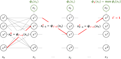
Figure 1: This schematic represents the Viterbi algorithm. At each step, the memorization table (denoted by $\psi_{i}(\cdot)$) and the logarithm posterior (denoted by $\phi_{i}(\cdot)$) are stored for all values of $i$, as detailed in Appendix -A. In this example, since the maximum value of $\phi_{i}(x_{T})$ occurs at $\phi_{i^{\ast}=1}(x_{T})$ at the final time $T$, the MAP sequence $x^{\text{MAP}}_{0:T}$ is decoded from the memorization table $\psi_{i^{\ast}=1}(x_{0:T})=\{x_{0}^{N},\ldots,x_{t-1}^{1},\ldots,x_{T-1}^{3},x_{T}^{1}\}$.

In general, finding $\phi^{\star}$ poses a challenging problem in functional optimization [38]. However, when $\phi$ is chosen from the unit ball of a vector-valued RKHS, denoted as $\mathcal{H}^{d}$, with a positive definite kernel $k(x,x^{\prime})$, the quest for $\phi^{\star}$ can be formulated as a manageable optimization task. This optimization entails maximizing the directional derivative of the Kullback-Leibler (KL) divergence with respect to $\phi$.

$$\phi\!^{\star}(x)\!=\!\arg\!\max_{\!\!\!\!\!\!\phi\in\mathcal{H}^{d}}\Bigl{\{}\text{D}_{\phi}\text{KL}[\,q(\epsilon\phi)\,\|\,p(x)\,]\,|\!\parallel\!\!\phi(x)\!\!\parallel_{\mathcal{H}^{d}}\leq 1\!\Bigl{\}},$$ (7)

where $q(\epsilon\phi)$ indicates the particle distribution resulting from taking an update step $x+\epsilon\phi(x)$. The optimization problem in (7) can have a closed-form solution via a connection to the kernelized Stein discrepancy (KSD) (Theorem 3.1. [28]),

$$\text{D}_{\phi}\text{KL}[\,q(\epsilon\phi)\,\|\,p(x)\,]=-\mathbb{E}_{q}[\textup{trace}(\mathcal{A}_{p}\phi(x))],$$ (8)

where $\mathcal{A}_{p}\phi(x):=\phi(x)\nabla_{x}\log p(x)^{\top}+\nabla_{x}\phi(x)$. Here, we use $\phi(x)$ in the Stein class of $p(x)$, for example, the Radial basis function (RBF) kernel [39]. The expectation term is estimated using the empirical mean of the particles $\{x^{i}\}_{i=1}^{N_{s}}$. Consequently, the optimal perturbation direction is computed as

$$\phi^{\star}(x)=\frac{1}{N_{s}}\sum_{i=1}^{N_{s}}(k(x^{i},x)\nabla_{x^{i}}\log p(x^{i})+\nabla_{x^{i}}k(x^{i},x)).$$ (9)

The first term in (9) is a weighted gradient of the $\log p(x)$, and the second term, known as the repulsive force, intuitively pushes particles apart when they approach each other closely, preventing them from collapsing into a single mode. This property is used to aid in the search for multiple MAP points within a multimodal distribution. Furthermore, $\nabla_{x}\log p(x)$ does not involve a normalization term, which is typically difficult to handle. This characteristic renders SVGD as a powerful technique for inferring intractable target distributions. Finally, the convergence of SVGD is guaranteed in the mean-field limit [28, 40].

III-C Second-order SVGD with Hessian-scaled Kernel

To enhance computational efficiency in our implementation, especially to reduce the number of iterations $K$, we propose incorporating curvature information using a Hessian-scaled RBF Kernel [41], $k(x,x^{\prime})=\exp\bigl{(}-\frac{1}{n_{x}}(x-x^{\prime})^{\top}M(x-x^{\prime})\bigl{)}$, where $M$ is the expected curvature approximated as $M=1/N_{s}\sum_{i=1}^{N_{s}}H(x^{i})$, with the Hessian matrix $H(x)=-\nabla_{x}^{2}\log p(x)$. As a result, the transport map in (6) is transformed into the following equation:

$$T(x)=x+\epsilon M^{-1}\phi(x).$$ (10)

This transformation significantly reduces the number of iterations $K$ required compared to the standard SVGD. In practice, the number of iterations $K$ is within the range of 10 to 50 [41].

IV Stein Variational Maximum A Posteriori Sequence Estimation

This section introduces our proposed MAP sequence estimation algorithm, Stein-MAP, presented in Algorithm 1. Stein-MAP is based on the formulation of sequential variational inference for MAP sequence estimation (2) of the dynamical system (1), incorporating SVGD with a Hessian-scaled Kernel.

When $p(x_{0:T}|z_{1:T})$ exhibits non-Gaussian and/or multimodal characteristics, it is impractical to represent in a closed form; thus, an approximation becomes essential. In the VI approach to solving the MAP problem, this entails using a proposal distribution $q(x_{0:T})$ to capture the underlying behavior of $p(x_{0:T}|z_{1:T})$. The relationship between $p(x_{0:T}|z_{1:T})$ and $q(x_{0:T})$ can be characterized using KL divergence (see details in Appendix -B):

$$\text{KL}[\,q(x_{0:T})\|\,p(x_{0:T}|z_{1:T})\,]=-\mathcal{L}(x_{0:T})+\log p(z_{1:T}),$$ (11)

where

$$\mathcal{L}(x_{0:T})=\int q(x_{0:T})\,\log\frac{p(x_{0:T},z_{1:T})}{q(x_{0:T})}dx_{0:T}$$ (12)

is known as the Evidence Lower BOund (ELBO).

IV-A Evidence Lower BOund (ELBO) with Dynamical System

The KL divergence in (11) is always nonnegative with equality to zero only happening when $q(x_{0:T})=p(x_{0:T}|z_{1:T})$. Therefore, as shown in the left-hand side of (11), the minimization of the KL divergence leads to an optimization problem for finding $q(x_{0:T})$ such that $q(x_{0:T})=p(x_{0:T}|z_{1:T})$. In many cases, the optimization problem is computationally infeasible. Therefore, we proceed with the optimization problem aimed at maximizing the ELBO as follows:

$$q^{\star}(x_{0:T})=\arg\!\max_{\!\!\!\!\!q(x_{0:T})}\mathcal{L}(x_{0:T}).$$ (13)

To address the above optimization problem, we need to handle both the log joint probability $\log p(x_{0:T},z_{1:T})$ and the proposal distribution $q(x_{0:T})$ in the ELBO. We factorize the log joint probability based on the Markov property and Assumption II.1 for observations $z_{1:T}$, as follows:

$$\log p(x_{0:T},z_{1:T})= \sum\nolimits_{t=1}^{T}\log p(z_{t}|x_{t})\,+$$

$$\sum\nolimits_{t=1}^{T}\log p(x_{t}|x_{t-1})+\log p(x_{0}).$$ (14)

Using (IV-A), the ELBO in (12) reads as

$$\mathcal{L}(x_{0:T}) =\int q(x_{0:T})\log p(x_{0})dx_{0:T}$$

$$~{}~{}~{}+\int q(x_{0:T})\sum\nolimits_{t=1}^{T}\log p(x_{t}|x_{t-1})dx_{0:T}$$

$$~{}~{}~{}+\int q(x_{0:T})\sum\nolimits_{t=1}^{T}\log p(z_{t}|x_{t})dx_{0:T}$$

$$~{}~{}~{}-\int q(x_{0:T})\log q(x_{0:T})dx_{0:T}.$$ (15)

Input : Transition probability $p(x_{t}|x_{t-1})$, prior $p(x_{0})$, likelihood function $p(z_{t}|x_{t})$, observations $z_{1:T}$, the number of particles $N_{s}$, the number of iteration steps $K$.

1 for $t=0,1,\dots,T$ do

2       if $t=0$ then

3             Initial particles, $\{x_{0,r}^{i}\}_{i=1}^{N_{s}}$ $\sim p(x_{0})$

4             for $i=1,2,\dots,N_{s}$ in parallel do

5                   $x_{0}^{i}\stackrel{{\scriptstyle K\text{steps}}}{{\longleftarrow}}x_{0}^{i}+\epsilon M^{-1}\phi^{\star}(x_{0}^{i})$,

6                   where $\phi^{\star}(x_{0})$ from $\eqref{eq::SVGD_updated_0_0}$

7             end for

8            $x_{0}^{\star}\stackrel{{\scriptstyle\eqref{eq::MAP_sequence decision_0}}}{{\longleftarrow}}\{x_{0}^{i}\}_{i=1}^{N_{s}}$

9       else

10             if $t=1$ then

11                  Initial particles, $\{x_{t}^{i}\}_{i=1}^{N_{s}}$ in $q^{\star}(x_{t-1})$

12             else

13                  Initial particles, $\{x_{t}^{i}\}_{i=1}^{N_{s}}$ in $q^{\star}(x_{t-1}|x_{t-2})$

14             end if

15            for $i=1,2,\dots,N_{s}$ in parallel do

16                   $x_{t}^{i}\stackrel{{\scriptstyle K\text{steps}}}{{\longleftarrow}}x_{t}^{i}+\epsilon M^{-1}\phi^{\star}(x_{t}^{i})$,

17                   where $\phi^{\star}(x_{t})$ from (24) given $x_{t-1}^{\star}$

18             end for

19            $x_{t}^{\star}\stackrel{{\scriptstyle\eqref{eq::MAP_sequence decision_1}}}{{\longleftarrow}}\{x_{t}^{i}\}_{i=1}^{N_{s}}$

20       end if

21      

22 end for

return $x^{\text{MAP}}_{0:T}=\{x_{0}^{\star},x_{1}^{\star},\dots,x_{T}^{\star}\}$

Algorithm 1 Stein-MAP algorithm

The VI literature employs two broad techniques to specify the joint proposal distribution $q(x_{0:T})$ in ELBO: selecting a manageable parametric form [43, 44, 45], or employing the mean field approximation [14]. The first approach involves using a parameterized distribution, such as an exponential family or Gaussian mixture model. In the second approach, the joint distribution is factorized into independent distributions for each time variable, i.e., $q(x_{0:T})=\prod_{t=0}^{T}q(x_{t})$. This factorization simplifies the optimization process at the cost of approximation accuracy. In this study, we adopt a mean-field-type approach, but with a weaker factorization assumption. Instead of assuming independence, we impose the Markov property for the proposal distribution.

Assumption IV.1 (Markov property on proposal distribution)

The proposal distribution $q(x_{0:T})$ in (13) is chosen such that

$$q(x_{t}|x_{t-1})=q(x_{t}|x_{t-1},x_{0:t-2}).$$ (16)

$\Box$

Under Assumption (IV.1), we can show that the optimal solution of (13) admits the following factorized structure.

Lemma IV.1 (The form of optimal proposal distribution)

Let Assumption IV.1 holds. Then, the optimal proposal distribution $q(x_{0:T})$ in (13) is factorized as

$$q(x_{0:T})=q(x_{0})\prod\nolimits_{t=1}^{T}q(x_{t}|x_{t-1}).$$ (17)

Proof:

See Appendix -C. ∎

According to Lemma IV.1, the proposal distribution $q(x_{0:T})$ is factorized in (IV-A). Consequently, we can write the ELBO in (13) as a summation of factorized KL divergence terms as stated in the results below.

Lemma IV.2 (The factorization of KL divergence)

Let Assumption II.1 and IV.1 holds. Then, ELBO (13) is factorized as

$$\mathcal{L}(x_{0:T})=-\text{KL}[\,q(x_{0})\,\|\,p(x_{0})\,]$$

$$\qquad\quad-\int\text{KL}[\,q(x_{1}|x_{0})\,\|\,p(z_{1}|x_{1})p(x_{1}|x_{0})]q(x_{0})dx_{0}$$

$$\qquad\quad-\sum\nolimits_{t=2}^{T}\int\text{KL}[\,q(x_{t}|x_{t-1})\,\|\,p(z_{t}|x_{t})p(x_{t}|x_{t-1})]$$

$$\qquad\qquad\qquad\qquad\qquad\qquad~{}~{}\times q(x_{t-1}|x_{t-2})dx_{t-1}.$$ (18)

Proof:

See Appendix -D. ∎

With the factorized representation given in (IV.2), we propose a computationally tractable (sub)optimal proposal distribution, as defined in (17), achieved through the minimization of the individual KL divergence terms and the associated marginalization term in (IV.2). In particular, when dealing with complex probability distributions that have multiple modes and cannot be expressed in closed form, we propose a particle-based solution approach using SVGD. As demonstrated in the experimental studies, this method has significant numerical efficiency.

IV-B Stein Variational MAP Sequence

The primary objective is to determine the MAP sequence, equivalent to (2), from

$$x_{0:T}^{\mathrm{MAP}}=\arg\!\max_{\!\!\!\!\!x_{0:T}}q^{\star}(x_{0:T}).$$ (19)

Given (13), this optimization problem can be represented as

$$(x_{0:T}^{\mathrm{MAP}},q^{\star}(x_{0:T}))=\arg\!\!\!\!\!\!\!\!\!\max_{\!\!\!\!\!\!x_{0:T}\in\mathcal{X},\;q(x_{0:T})}\hat{\mathcal{L}}(x_{0:T}),$$ (20)

where $\mathcal{X}$ is the candidate set of MAP sequences. Using SVGD, which enables a particle-based approximation to the proposal distribution with $N_{s}$ particles $\{x^{i}\}_{i=1}^{N_{s}}$, i.e., $q(x)=\frac{1}{N_{s}}\sum\nolimits_{i=1}^{N_{s}}\delta(x-x^{i})$, we develop a sequential variational inference framework to solve (20). Given $\{x^{i}\}_{i=1}^{N_{s}}$ in $q(x)$, $\hat{\mathcal{L}}(x_{0:T})$ is derived from (IV.2) as

$$\hat{\mathcal{L}}(x_{0:T})=-\text{KL}[\,q(x_{0})\,\|\,p(x_{0})\,]$$

$$-\!\sum\nolimits_{t=1}^{T}\!\frac{1}{N_{s}}\!\sum\nolimits_{j=1}^{N_{s}}\text{KL}[\,q(x_{t}|x_{t-1}^{j})\,\|\,p(z_{t},x_{t}|x_{t-1}^{j})].$$ (21)

where $p(z_{t},x_{t}|x_{t-1}^{j})=p(z_{t}|x_{t})p(x_{t}|x_{t-1}^{j})$ represents the joint probability of $z_{t}$ and $x_{t}$ given the previous state $x_{t-1}^{j}$. The inner summation term in the subtrahend of (IV-B) approximates the integration terms in (IV.2). The term $1/N_{s}$, obtained from either $q(x_{0})$ or $q(x_{t-1}|x_{t-2})$, can be taken out from the summation.

To solve (20) with 2 unknowns $q^{\star}$ and $x^{\mathrm{MAP}}$ at each time $t$, we propose the following iterative approach:

• finding the optimal distribution $q^{\star}$ given $x_{t-1}^{\star}$ and

• determining the MAP solution $x_{t}^{\star}$ to minimize KL divergence given the optimal distribution $q^{\star}$.

Consequently, the MAP sequence is obtained sequentially from the following steps. First, starting at the initial time step, $t=0$, and given $p(x_{0})$, we compute $q^{\star}(x_{0})=\frac{1}{N_{s}}\sum\nolimits_{i=1}^{N_{s}}\delta(x_{0}-x_{0}^{i})$ where $x_{0}^{i}$ is obtained via (10) from

$$\phi^{\star}(x_{0})=\frac{1}{N_{s}}\sum_{i=1}^{N_{s}}(k(x_{0}^{i},x_{0})\nabla_{x_{0}^{i}}\log p(x_{0}^{i})+\nabla_{x_{0}^{i}}k(x_{0}^{i},x_{0})).$$ (22)

Then, $x_{0}^{\star}$ is chosen from the set $\{x_{0}^{i}\}_{i=1}^{N_{s}}$ in $q^{\star}(x_{0})$ to minimize KL divergence at time $t=0$ in (IV-B) using

$$x_{0}^{\star}=\arg\!\!\!\!\!\!\max_{\!\!\!\!x_{0}\in\{x_{0}^{i}\}_{i=1}^{N_{s}}}\;p\bigl{(}x_{0}^{i}\bigl{)}.$$ (23)

Subsequently, at each time step $t\geq 1$, given the previous $x_{t-1}^{\star}$, we propose computing the optimal distribution $q^{\star}(x_{t}|x_{t-1})=\frac{1}{N_{s}}\sum\nolimits_{i=1}^{N_{s}}\delta(x_{t}-x_{t}^{i})$ where $x_{t}^{i}$ is obtained via (10) from

$$\phi^{\star}(x_{t})=\phi^{\star}(x_{t}|x_{t-1}^{\star})\cdot\delta(x_{t-1}-x^{\star}_{t-1}),\quad t\geq 1,$$ (24)

where

$$\phi^{\star}(x_{t}|x_{t-1}^{\star})\!\!=\frac{1}{N_{s}}\sum_{i=1}^{N_{s}}\Big{(}k(x_{t}^{i},x_{t})\nabla_{x_{t}^{i}}\log\bigl{(}p(z_{t}|x_{t}^{i})p(x_{t}^{i}|x_{t-1}^{\star})\bigl{)}$$

$$\qquad\qquad\qquad\qquad\qquad\qquad\qquad\qquad\quad~{}+\nabla_{x_{t}^{i}}k(x_{t}^{i},x_{t})\Big{)}.$$

then, given $\{x_{t-1}^{j}\}_{j=1}^{N_{s}}$ from the previous $q^{\star}$, we select $x_{t}^{\star}$ from the set $\{x_{t}^{i}\}_{i=1}^{N_{s}}$ in $q^{\star}(x_{t}|x_{t-1})$ to minimize KL divergence at time $t$ in (IV-B) using the following formula:

$$x_{t}^{\star}=\arg\!\!\!\!\!\max_{\!\!\!\!x_{t}\in\{x_{t}^{i}\}_{i=1}^{N_{s}}}\;\frac{1}{N_{s}}\sum\nolimits_{j=1}^{N_{s}}p(z_{t},x_{t}^{i}|x_{t-1}^{j}),$$ (25)

where $p(z_{t},x_{t}^{i}|x_{t-1}^{j})=p(z_{t}|x_{t}^{i})p(x_{t}^{i}|x_{t-1}^{j})$.

The term $\phi^{\star}(x_{t}|x_{t-1}^{\star})$ in (24) defines the gradient flow that originates from the previous MAP point $x_{t-1}^{\star}$. This modification ensures that $q^{\star}(x_{t}|x_{t-1})$ is computed based on the maximum state $x_{t-1}^{\star}$, resulting in differences compared to the posterior of the Stein particle filter [32]. Detailed results will be presented in the experimental demonstrations in Section V.

Next, we show that a MAP sequence $x^{\text{MAP}}_{0:T}$ is the unique solution to the optimization problem defined in (20) with (IV-B). The underlying assumptions that ensure the uniqueness of the MAP sequence are as follows.

Assumption IV.2 (Assumption on particles)

In the optimization problem (20) with (IV-B), given the set of $N_{s}$ particles $\{x^{1},\dots,x^{N_{s}}\}$ in $q^{\star}$, for any pair of particles indexed by $i$ and $j$ ($i,j\in{1,\dots,N_{s}}$), the following condition is satisfied:

$$x^{i}\neq x^{j}\quad\text{for all}\quad i\neq j.$$ (26)

$\Box$

This assumption simply states that the $N_{s}$ particles do not overlap at a given $q^{\star}$. The following assumption states the shape of the multimodal distribution when the conditional joint probability $p(x_{t},z_{t}|x_{t-1})$ is multimodal.

Assumption IV.3 (Assumption on $p(x_{t},z_{t}|x_{t-1})$)

In the optimization problem (20) with (IV-B), when considering observation $z_{t}$, there are no alternative probability distributions, denoted $p(x_{t},z_{t}|x_{t-1})$, within the entire state space $x_{t}$ and $x_{t-1}$ that share modes of equal height with the distribution under consideration. $\Box$

Under the above assumptions, the next result shows that the optimization problem in (20) with (IV-B) for the MAP sequence has a unique solution.

Theorem IV.1 (Uniqueness of MAP sequence)

Let Assumptions IV.2 and IV.3 holds and assume $p(x_{0})$ is unimodal. Then, given $q^{\star}$, there exists a unique solution $x_{0:T}^{\mathrm{MAP}}$ in the optimization problem (20) with (IV-B), for all $x_{0:T}\in\mathcal{X}$ such that

$$\hat{\mathcal{L}}(x_{0:T}^{\mathrm{MAP}})\geq\hat{\mathcal{L}}(x_{0:T})\quad\text{for all}\quad x_{0:T}\in\mathcal{X},$$ (27)

where equality if and only if $x_{0:T}=x_{0:T}^{\mathrm{MAP}}$. $\Box$

Proof:

By the definition of the KL divergence, we can express $\hat{\mathcal{L}}(x_{0:T})$ of (IV-B) as follows:

$$\hat{\mathcal{L}}(x_{0:T})=-\frac{1}{N_{s}}\Bigl{(}\log q^{\star}(x_{0})-\log p(x_{0})\Bigl{)}$$

$$-\sum_{t=1}^{T}\sum_{j=1}^{N_{s}}\frac{1}{N_{s}^{2}}\Bigl{(}\log q^{\star}(x_{t}|x_{t-1}^{j})-\log p(x_{t},z_{t}|x_{t-1}^{j})\Bigl{)},$$ (28)

where the $1/N_{s}$ term originates from $q^{\star}$ in the KL divergence. Assumption IV.2 and Assumption IV.3 ensure that particles in $q^{\star}$ do not overlap, and there are no other probability distributions with modes of the same height within the state space. As a result, we can conclude that $x_{t}$, chosen to minimize each KL divergence given $\{x_{t-1}^{j}\}_{j=1}^{N_{s}}$ from a previous $q^{\star}$ at each time step $t$ in $\hat{\mathcal{L}}(x_{0:T})$, has a unique MAP solution.

Therefore, there exists a unique solution $x_{0:T}^{\mathrm{MAP}}$ that maximizes $\hat{\mathcal{L}}(x_{0:T})$, satisfying (27), for all $x_{0:T}\in\mathcal{X}$. ∎

According to Theorem IV.1, the optimization problem (20) with (IV-B) is solved by selecting $x_{t}^{\star}$ from the set $\{x_{t}^{i}\}_{i=1}^{N_{s}}$ in $q^{\star}$ to minimize the KL divergence at each time step $t$.

Remark IV.1

In practical scenarios, Assumption IV.2 is frequently observed, especially when the number of particles is not exceedingly large. This condition is facilitated by the presence of a repulsive force, denoted by the second term in (9). Furthermore, proper selection of the transition probability $p(x_{t}|x_{t-1})$ leads to a high likelihood of satisfying Assumption IV.3. This will be demonstrated in the experimental results presented in Section V. $\Box$

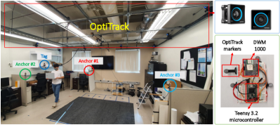
Figure 2: Experimental setup: the OptiTrack system, equipped with 12 infrared cameras, provided precise localization results with an accuracy of $10^{-4}\,$m. In the 2D localization setup, the tag, positioned by a moving agent, was maintained at a consistent height, while three anchors were placed within an indoor environment ($8\,$m $\times 8\,$m) at the same height. This arrangement ensures an unobstructed line of sight between the anchors and the tag, minimizing the potential for biased range measurements.

Remark IV.2

In contrast to the Viterbi algorithm, which exhaustively searches with a time complexity of $O(N^{2})$, where $N$ is the number of discrete states (particles), Stein-MAP finds a candidate for $x^{\mathrm{MAP}}$ using a deterministic gradient flow with few iteration steps. As a result, the computational complexity is reduced to $O(N)$. Since SVGD requires a small number of $N$ particles to compute $q^{\star}$, it exhibits an efficient computational performance. $\Box$

In summary, we sequentially obtain the MAP sequence without the need to maintain all candidate sequences, similar to the memorization table and backtracking process used in the Viterbi algorithm. Furthermore, particles are deterministically identified with minimal iteration steps ($K=10$ to $50$) using second-order (curvature) information. These approaches significantly reduce computational and memory burdens.

V Experimental Demonstrations

This section examines the effectiveness of the Stein-MAP method in the field of robotics, particularly in the difficult task of range-only localization. In range-only localization, the objective is to estimate the position of an object or receiver solely based on distance measurements between the object and multiple reference points, commonly referred to as anchors. This technique is widely applied in various domains, including robotics, autonomous vehicles, and wireless sensor networks [47, 48, 49]. Range-only localization offers several advantages, including simplicity, cost-effectiveness, and suitability for environments where GPS may not be accessible, such as indoors and underwater. However, it also has limitations, including the need for an adequate number of anchors, susceptibility to measurement errors, and the potential for multiple local optimum solutions (multimodality). Our proposed method demonstrates an effective solution to these challenges. Experimental studies are also used to compare the accuracy of Stein-MAP estimation to other existing methods.

We localize a target that is not equipped with any proprioceptive sensor, such as IMU or encoders. Consequently, we use a transition probability of (1) as follows:

$$p(x_{t}|x_{t-1};\zeta)\propto\exp\biggl{(}-\frac{\|x_{t}-x_{t-1}\|_{2}^{2}}{2\zeta^{2}}\biggl{)},$$ (29)

where parameter $\zeta\in{\mathbb{R}}_{>0}$ denotes the predefined standard deviation in the assumed motion model. The transition probability provides the conditional probability of the position variable $x_{t}$ given the previous position $x_{t-1}$ while accounting for the inherent temporal dependencies among the position variables (zero velocity model).

In addition, we consider line-of-sight (LoS) range measurements, thus formulating the likelihood function of the range measurement in (1) as follows:

$$p(z_{t}|x_{t};\theta)\propto\prod_{\forall l}\exp\biggl{(}-\frac{\|z_{t,l}\,-\,\Gamma_{l}(x_{t})\|_{2}^{2}}{2\sigma_{z,l}^{2}}\biggl{)},$$ (30)

where $z_{t,l}\in{\mathbb{R}}_{\geq 0}$ represents the measurement value from the $l$-th anchor $P_{l}$ at time index $t$, and the product arises from the assumption of independent and identically distributed (i.i.d.) measurements. Here, $\forall l$ denotes all connected anchors. $\Gamma_{l}(x_{t})$ is a function of Euclidean distance, that is, $\Gamma_{l}(x_{t})=\|x_{t}-P_{l}\|_{2}$, which leads to nonlinearity. $\sigma_{z,l}\in{\mathbb{R}}_{>0}$ is the standard deviation of measurement $z_{t,l}$. Here, the parameter vector $\theta=[P_{l},~{}\sigma_{z,l}]$ is given and/or predefined.

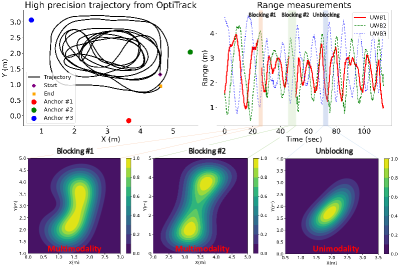
Figure 3: An agent traversed an arbitrary trajectory captured using the OptiTrack system at a rate of $120$ Hz, while the UWB sensor provided range measurements at $10$ Hz. During the experiment ($114.5s$), a tag and three anchors were fully connected except for the blocking periods. We blocked anchor #1 twice at specific times (referred to as Blocking #1 and #2), resulting in a connection only to anchors #2 and #3. The contour plots of the likelihood function (30) for the periods of Blocking #1 ($t=28.5s$) and Blocking #2 ($t=52.9s$) displayed a multimodal distribution, whereas Unblocking ($t=74.0s$) exhibited an unimodal distribution.

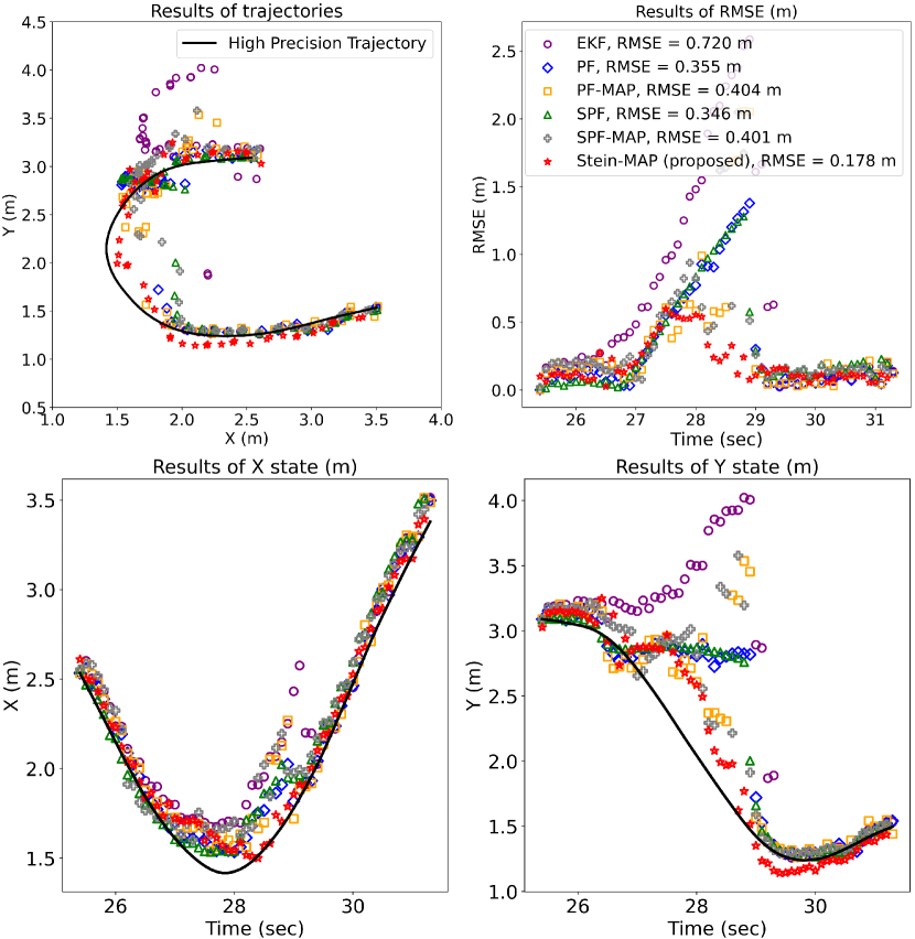
(a) Blocking #1 ($z_{t,l=1}$ dropped in $t\in[27,~{}29.5]s$)

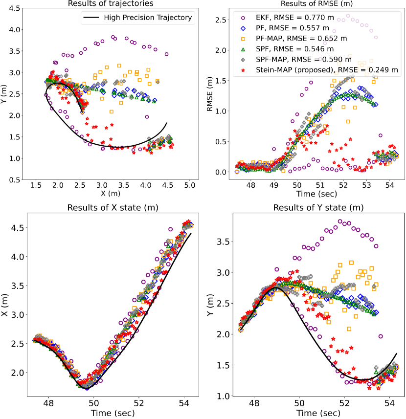
(b) Blocking #2 ($z_{t,l=1}$ dropped in $t\in[49,~{}54]s$)

Figure 4: The Estimated Position results ($10\,$Hz) and RMSE comparison among methods during Blocking #1 and #2 periods.

V-A Experimental Settings and Parameters

In our experiment, a human agent equipped with an Ultra-wideband (UWB) transceiver (tag) walked along an arbitrary trajectory in an $8\,$m $\times 8\,$m indoor environment (Cooperative System Lab at UC Irvine) with 3 UWB anchors. Here, UWB provides range measurements at 10 Hz and can also communicate their IDs, eliminating the need for data association considerations. There were no obstacles between the anchors and tag to mitigate the biased range measurements, as shown in Fig 2. In practice, some anchors might be blocked by dynamic or static obstacles, resulting in multimodal distribution (underdetermined nature of distance measurements). In the experiment, we dropped measurements from anchor #1 at specific time instances to simulate real-world (underdetermined) scenarios for robustness analysis against multimodality, see Fig 3. We used a DWM 1000 module alongside a Teensy 3.2 microcontroller for data acquisition. The microcontroller contains embedded sensor data communication software, allowing us to log and synchronize measurement data using timestamps. For a precise reference trajectory comparison, we employed the OptiTrack optical motion capture system with a mobile agent equipped with four markers. This OptiTrack system utilizes 12 infrared cameras to achieve high precision localization with an accuracy of $10^{-4}\;$m, and a sampling rate of $120$ Hz.

The parameters of the dynamical system model were configured as follows: $\zeta=1.0$ to account for the agent’s movement, and $\sigma_{z}=0.5\,$m to incorporate measurement error and address a minor range bias. Note that the UWB sensor, due to its high accuracy (range measurement error $<0.1$ to $0.3\,$m according to UWB models), can readily exhibit multimodality when the number of connections is insufficient.

V-B Performance Evaluation and Discussion

We conducted a performance comparison with several state estimation methods, including the Extended Kalman filter (EKF) [2], particle filter (PF) [4], Particle-based filter MAP estimate (PF-MAP) [24], Stein particle filter (SPF) [32], and Stein particle filter MAP estimate (SPF-MAP). Detailed descriptions of these methods are provided in Appendix -E. We implemented the estimation methods in a Python environment on a laptop with an Intel i7-10510U CPU and 32GB of RAM.

In this experiment, it was assumed that the initial position was known. Consequently, for the EKF, we set the initial covariance as $\Xi_{0}=0.5\times\mathsf{I}_{2\times 2}$, where $\mathsf{I}$ denotes the identity matrix. For PF and PF-MAP, we employed $N_{p}=1000$ particles, wherease for SPF, SPF-MAP, and Stein-MAP, we used $N_{s}=40$ particles with $K=25$ iterations.

V-B1 Estimation Accuracy Evaluation

We evaluated the accuracy of our positioning estimates using high-precision position data and employed the root mean squared error (RMSE) metric for quantification. Figure 4 displays the estimated position (10Hz), RMSE values, and estimated $x$ and $y$ states generated by each method for both (a) Blocking #1 and (b) Blocking #2. As depicted in the figure, the high-precision trajectories for Blocking #2 exhibit significant deviations compared to those for Blocking #1, posing challenges for the estimation accuracy. Furthermore, we employed contour plots to visualize the posterior results of each method at specific time points, see Fig 5.

First, we observed that the EKF accuracy degrades during the blocking time, with RMSE values of (a) $0.720\,$m and (b) $0.770\,$m. This degradation is attributed to the limitations of Gaussian-based MMSE state estimators when dealing with multimodal posterior distributions, which often lead to convergence toward a single mode. We examined this outcome by analyzing the contour plot of the posterior distribution shown in Fig 5. In contrast, the PF method, which is capable of managing non-Gaussian distributions with weighted particles, exhibited lower RMSE values than the EKF [(a) $0.355\,$m, (b) $0.557\,$m]. Nonetheless, it had limitations in fully addressing multimodality. This is because the PF utilizes the transition model as a proposal distribution for implementing importance sampling (Bootstrap filter), which results in particle weights that align with the inherently multimodal nature of the likelihood, as illustrated in Fig. 5. While PF-MAP exhibited enhanced performance in handling multimodality at specific points compared to PF (with a lower RMSE than PF during the blocking period), it experienced instability during the unblocking period, resulting in less favorable outcomes compared to MMSE result of PF with RMSE values of (a) $0.404,$m and (b) $0.652,$m. In the case of SPF and SPF-MAP, despite using fewer particles (specifically, $N_{s}=40$), they outperformed both PF and PF-MAP (with $N_{p}=1000$) in terms of accuracy, achieving RMSE values of (a) $0.346\,$m and (b) $0.546\,$m. When comparing the contour plots, it became evident that the posterior based on SVGD, which deterministically locates particles, captures the prior model information better than PF. Based on this, SPF-MAP exhibited superior performance compared to PF-MAP but still performed less favorably than SPF [(a) $0.401\,$m and (b) $0.590\,$m]. Our proposed Stein-MAP method had the highest estimation accuracy among all evaluated methods, with RMSE values of (a) $0.178\,$m and (b) $0.249\,$m. In Stein-MAP, particle updates rely on the previous maximum state, resulting in a more robust posterior than SPF for handling the multimodal nature of likelihood. The contour plots verified that Stein-MAP posterior exhibits a single mode, with particles concentrated in this mode, leading to the highest estimation results.

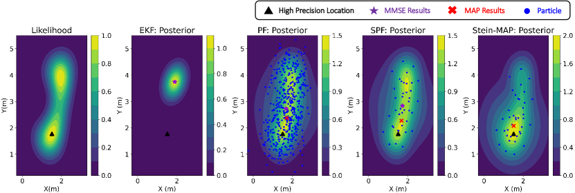
(a) Contour Plots @ $t=29.0s$ during Blocking #1 period

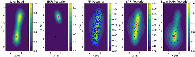
(b) Contour Plots @ $t=52.9s$ during Blocking #2 period

Figure 5: Contour plots of the Posterior for each method during Blocking #1 and #2 periods.

V-B2 Robustness Evaluation

To assess robustness against multimodality, we extended the blocking period from three to seven, denoted as Block (BL) #Number as shown in Table I. The blocking times are BL #3 ($63.0$ to $67.0$s), BL #4 ($75.0$ to $79.0$s), BL #5 ($82.0$ to $85.0$s), BL #6 ($91.0$ to $94.0$s), and BL #7 ($99.5$ to $103.0$s). We calculated the average RMSE metric over $10$ runs to reduce the impact of sampling variations. Table II demonstrates that our proposed Stein-MAP maintains a consistent RMSE even as the number of blocking increases, compared with the other methods.

TABLE I: Experiment Setup: Blocking (BL) Period

	BL#1	BL#2	BL#3	BL#4	BL#5	BL#6	BL#7
BL Time	$2.5$s	$5.0$s	$4.0$s	$4.0$s	$3.0$s	$3.0$s	$3.5$s
Exp #1	O	O	O	-	-	-	-
Exp #2	O	O	O	O	-	-	-
Exp #3	O	O	O	O	O	-	-
Exp #4	O	O	O	O	O	O	-
Exp #5	O	O	O	O	O	O	O

TABLE II: Robustness Evaluation, average RMSE (m) over $10$ runs

	EKF	PF	PF-MAP	SPF	SPF-MAP	Stein-MAP (proposed)
Exp #1	0.294	0.211	0.218	0.204	0.211	$\mathbf{0.204}$
Exp #2	0.295	0.242	0.254	0.220	0.212	$\mathbf{0.208}$
Exp #3	0.296	0.253	0.261	0.232	0.224	$\mathbf{0.212}$
Exp #4	0.325	0.262	0.278	0.240	0.232	$\mathbf{0.217}$
Exp #5	0.326	0.274	0.282	0.255	0.251	$\mathbf{0.218}$

TABLE III: Estimation Error as Particle Count: RMSE (m)

No. of particles	5	10	20	40
Exp #1	0.295	0.167	0.321	0.204
Exp #2	0.262	0.167	0.328	0.208
Exp #3	0.275	0.175	0.346	0.212
Exp #4	0.312	0.185	0.347	0.217
Exp #5	0.313	0.201	0.358	0.218

V-B3 Particle Count-based Estimation Accuracy Evaluation

We evaluated the estimation accuracy of Stein-MAP using different particle numbers, ranging from $5$ to $40$, as summarized in Table III. When employing only $5$ particles, as shown in Fig 6, it became evident that this number was insufficient to represent the distribution accurately, leading to increased estimation errors. Our experiments revealed that the use of $10$ particles resulted in the highest accuracy. However, during the introduction of Block #7 period, the error increased rapidly. This observation was supported by the contour plot, highlighting the inadequacy of the particles in accurately representing the distribution. Interestingly, employing $20$ particles yielded the worst accuracy, as it tended to converge toward other modes even more than when using $10$ particles. This behavior can be attributed to the limited number of particles, which hampers their ability to converge to all mode points owing to repulsive forces. The use of more than $40$ particles consistently produced estimation errors. This was because a sufficient number of particles effectively represented the distribution, covering the entire range of mode points and facilitating the successful sequential identification of MAP points.

V-B4 Discussion of Run-Time Performance

In [32], it was demonstrated that the run-time was impressively short, measured in milliseconds, when employing a C++ implementation on an Intel Core i7-7700 CPU with 16GB of RAM. In terms of computational complexity, although our proposed Stein-MAP involves an additional step for locating MAP points as defined in (25), it is noteworthy that SVGD requires a relatively small number of particles (e.g., $N_{s}=40$). Moreover, if we opt for a binary search, additional computational complexity remains at manageable $O(\log N_{s})$. In our Python environment, the run-time of a single time-step of our proposed Stein-MAP was shorter than those of SPF and SPF-MAP. This improvement in run-time can be attributed to the calculation of $\phi^{\star}(x_{t})$ using only one previous state $x_{t-1}^{\star}$ instead of $N_{s}$ $i$-th states $x_{t-1}^{i}$.

VI Conclusion and Future Work

State estimation in robotics is a significant challenge that often involves complex scenarios and multimodal distributions in the real world. Our estimation methods aim to handle these multimodal distributions efficiently. In this article, we introduced a MAP sequence estimation method that effectively manages multimodality while reducing computational and memory requirements. This approach is grounded in a sequential variational inference framework, that considers dependencies between transition states over time within dynamic system models. Building on this foundation, we tackled MAP sequence estimation through a deterministic gradient flow of particles, embedded in a reproducing kernel Hilbert space. To validate our methods, we conducted real-world experiments, with a particular focus on range-only (wireless) localization. Additionally, we conducted a comprehensive analysis encompassing robustness, impact of particle count, and run-time performance. In a future study, we plan to integrate adaptive prior models into the current estimation framework to enhance its robustness in handling multimodal distributions. In addition, we will address active sensing, with a specific emphasis on motion planning.

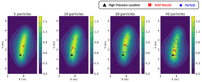
Figure 6: Contour plots of the Posterior according to Particle Count @ $t=101.5s$ during Blocking #7 period.

-A The outline of the Viterbi algorithm

Let $x_{t}^{1},\cdots,x_{t}^{N}$ be $N$ discrete samples representing the state space of the system at time $t$. At the initial step $t=1$, given $p(x_{0})$, for the $i$-th state $x_{1}^{i}$, $i\in\{1,\dots,N\}$, the Viterbi algorithm obtains the most probable state $\psi_{i}(x_{1})$ and logarithm posterior $\phi_{i}(x_{1})$ as follows:

$$\psi_{i}(x_{1}) =x_{0},~{}~{}~{}\forall i\in\{1,\dots,N\},$$

$$\phi_{i}(x_{1}) =\;\log\bigl{(}p(z_{1}|x_{1}^{i})\times p(x_{1}^{i}|x_{0})\times p(x_{0})\bigl{)},~{}~{}~{}\forall i.$$

Then, at each time step $t>1$, for each given $i$-th state $x_{t}^{i}$, $\psi_{i}(x_{t})$ and $\phi_{i}(x_{t})$ are computed from

$$\psi_{i}(x_{t})=\arg\!\max_{x_{t-1}^{j}}\log\bigl{(}p(x_{t}^{i}|x_{t-1}^{j})\bigl{)}+\phi_{j}(x_{t-1}),~{}\forall i,$$

$$\phi_{i}(x_{t})\!=\!\log\Bigl{(}p\bigl{(}z_{t}|x_{t}^{i}\bigl{)}\!\times p\bigl{(}x_{t}^{i}|\psi_{i}(x_{t})\bigl{)}\Bigl{)}+\phi_{j^{\star}}(x_{t-1}),~{}\forall i,$$

where $j^{\star}$ is associated with $x_{t-1}^{j^{\star}}$ through the relation $\psi_{i}(x_{t})=x_{t-1}^{j^{\star}}$, and these processes are implemented recursively until the final time $T$. Finally, the MAP sequence $x_{0:T}^{\text{MAP}}$ is decoded from the memorization table, $\psi_{i^{\ast}}(x_{0:T})$, by backtracking process from $i^{\ast}$ (see an example in Fig 1.) as follows

$$x_{T}^{i^{\ast}}=\arg\!\max_{x_{T}}\phi_{i}(x_{T}).$$

-B The derivation of the ELBO

To address the connection between $p(x_{0:T}|z_{1:T})$ and $q(x_{0:T})$, the representation of the log-posterior $\log p(x_{0:T}|z_{1:T})$ can be established using the relationship between joint and conditional probabilities given by

$$\log p(x_{0:T}|z_{1:T})=\log p(x_{0:T},z_{1:T})-\log p(z_{1:T}),$$ (33)

The proposal distribution $q(x_{0:T})$ is then introduced by subtracting of $\log q(x_{0:T})$ from both sides of (33), that is,

$$\log\frac{p(x_{0:T}|z_{1:T})}{q(x_{0:T})}=\log\frac{p(x_{0:T},z_{1:T})}{q(x_{0:T})}-\log p(z_{1:T}).$$ (34)

Note that the expectation of both sides of (34) w.r.t. $q(x_{0:T})$,

$$\int q(x_{0:T})\,\log\frac{p(x_{0:T}|z_{1:T})}{q(x_{0:T})}dx_{0:T}$$

$$~{}~{}=\int q(x_{0:T})\,\log\frac{p(x_{0:T},z_{1:T})}{q(x_{0:T})}dx_{0:T}-\log p(z_{1:T}),$$ (35)

where $\log p(z_{1:T})$ on the right-hand side of (-B) is independent of $x_{0:T}$. Therefore, $\int q(x_{0:T})\log p(z_{1:T})dx_{0:T}=\log p(z_{1:T})$. Moreover, the left-hand side of (-B) can be expressed using the KL divergence:

$$\text{KL}[\,q(x_{0:T})\,\|\,p(x_{0:T}|z_{1:T})\,]$$ (36)

$$=-\int q(x_{0:T})\,\log\frac{p(x_{0:T},z_{1:T})}{q(x_{0:T})}dx_{0:T}+\log p(z_{1:T})\geq 0.$$

-C Proof of Lemma 4.1

Proof:

The optimal distribution $q^{\star}(x_{0:T})$ is given as

$$q^{\star}(x_{0:T})=\arg\!\max_{\!\!\!\!\!q(x_{0:T})}\mathcal{L}(x_{0:T}),$$ (37)

where

$$\mathcal{L}(x_{0:T}) =\int q(x_{0:T})\log p(x_{0})dx_{0:T}$$

$$~{}~{}~{}~{}+\int q(x_{0:T})\sum\nolimits_{t=1}^{T}\log p(x_{t}|x_{t-1})dx_{0:T}$$

$$~{}~{}~{}~{}+\int q(x_{0:T})\sum\nolimits_{t=1}^{T}\log p(z_{t}|x_{t})dx_{0:T}$$

$$~{}~{}~{}~{}-\int q(x_{0:T})\log q(x_{0:T})dx_{0:T}.$$ (38)

The last integral term in (-C) can be represented by

$$- \int q(x_{0:T})\log q(x_{0:T})dx_{0:T}=-\int q(x_{0})\log q(x_{0})dx_{0}$$

$$~{}~{}~{}~{}-\sum\nolimits_{t=2}^{T}\int q(x_{0:T})\log q(x_{t}|x_{t-1},x_{0:t-2})dx_{0:T}.$$ (39)

Using the conditional differential entropy [50] as given by

$$-\int\!\!\!\int p(x,y)\log p(x|y)dxdy\leq-\int p(x)\log p(x)dx,$$ (40)

where equality if and only if $x$ and $y$ are independent, we have

$$-\int q(x_{0:T})\log q(x_{t}|x_{t-1},x_{0:t-2})dx_{0:T}$$

$$\leq-\int q(x_{0:T})\log q(x_{t}|x_{t-1})dx_{0:T}.$$ (41)

Under Assumption IV.1, there exists

$$q(x_{t}|x_{t-1})=q(x_{t}|x_{t-1},x_{0:t-2}),$$ (42)

and thus $q(x_{0:T})$ is given via (-C) as

$$q(x_{0:T})=q(x_{0})\prod\nolimits_{t=1}^{T}q(x_{t}|x_{t-1}).$$ (43)

∎

-D Proof of Lemma 4.2

Under Lemma IV.1, and considering that $\log p(x_{t}|x_{t-1})$ and $\log p(z_{t}|x_{t})$ depend solely on $x_{t}$ and/or $x_{t-1}$ of $x_{0:T}$, the ELBO in (13) is derived from (IV-A):

$$\mathcal{L}(x_{0:T}) =\int q(x_{0})\log p(x_{0})dx_{0}$$

$$~{}~{}~{}~{}+\sum\nolimits_{t=1}^{T}\int q(x_{t:t-1})\log p(x_{t}|x_{t-1})dx_{t:t-1}$$

$$~{}~{}~{}~{}+\sum\nolimits_{t=1}^{T}\int q(x_{t})\log p(z_{t}|x_{t})dx_{t}$$

$$~{}~{}~{}~{}-\int q(x_{0:T})\log\biggl{(}q(x_{0})\prod\nolimits_{t=1}^{T}q(x_{t}|x_{t-1})\biggl{)}dx_{0:T}$$

$$=\int q(x_{0})\log p(x_{0})dx_{0}-\int q(x_{0})\log q(x_{0})dx_{0}$$

$$~{}~{}~{}~{}+\sum\nolimits_{t=1}^{T}\int q(x_{t:t-1})\log p(x_{t}|x_{t-1})dx_{t:t-1}$$

$$~{}~{}~{}~{}+\sum\nolimits_{t=1}^{T}\int q(x_{t})\log p(z_{t}|x_{t})dx_{t}$$

$$~{}~{}~{}~{}-\!\sum\nolimits_{t=1}^{T}\!\!\int\!q(x_{t:t-1})\log q(x_{t}|x_{t-1})dx_{t:t-1}.$$ (44)

Next, we apply the marginalization technique and the law of total probability to demonstrate that the ELBO in (-D) can be represented recursively as follows:

$$\mathcal{L}(x_{0:T})=\int q(x_{0})\log p(x_{0})dx_{0}-\int q(x_{0})\log q(x_{0})dx_{0}$$

$$~{}~{}+\int q(x_{1}|x_{0})q(x_{0})\log p(x_{1}|x_{0})dx_{1:0}$$

$$~{}~{}+\sum\nolimits_{t=2}^{T}\int q(x_{t}|x_{t-1})q(x_{t-1},x_{t-2})\log p(x_{t}|x_{t-1})dx_{t:t-2}$$

$$~{}~{}+\int q(x_{1}|x_{0})q(x_{0})\log p(z_{1}|x_{1})dx_{1:0}$$

$$~{}~{}+\sum\nolimits_{t=2}^{T}\int q(x_{t}|x_{t-1})q(x_{t-1},x_{t-2})\log p(z_{t}|x_{t})dx_{t:t-2}$$

$$~{}~{}-\int q(x_{1}|x_{0})q(x_{0})\log q(x_{1}|x_{0})dx_{1:0}$$

$$~{}~{}-\sum\nolimits_{t=2}^{T}\!\!\int q(x_{t}|x_{t-1})q(x_{t-1},x_{t-2})\log q(x_{t}|x_{t-1})dx_{t:t-2}.$$ (45)

Each term is rearranged depends on $x_{0}$, $x_{1:0}$, and $x_{t:t-2}$, respectively, then the ELBO term can be expressed by

$$\mathcal{L}(x_{0:T})=\int q(x_{0})\biggl{(}\log p(x_{0})-\log q(x_{0})\biggl{)}dx_{0}$$

$$+\int\biggl{(}\int q(x_{1}|x_{0})\Bigl{(}\log p(x_{1}|x_{0})+\log p(z_{1}|x_{1})$$

$$\qquad\qquad\qquad\qquad\qquad-\log q(x_{1}|x_{0})\Bigl{)}dx_{1}\biggl{)}q(x_{0})dx_{0}$$

$$+\sum\nolimits_{t=2}^{T}\int\biggl{(}\int q(x_{t}|x_{t-1})\Bigl{(}\log p(x_{t}|x_{t-1})+\log p(z_{t}|x_{t})$$

$$\qquad-\log q(x_{t}|x_{t-1})\Bigl{)}dx_{t}\biggl{)}q(x_{t-1}|x_{t-2})q(x_{t-2})dx_{t-1:t-2}.$$ (46)

Using the definition of KL divergence, the ELBO can be represented by

$$\mathcal{L}(x_{0:T})=-\text{KL}[\,q(x_{0})\,\|\,p(x_{0})\,]$$

$$-\int\text{KL}[\,q(x_{1}|x_{0})\,\|\,p(z_{1}|x_{1})p(x_{1}|x_{0})]q(x_{0})dx_{0}$$

$$-\sum\nolimits_{t=2}^{T}\int\text{KL}[\,q(x_{t}|x_{t-1})\,\|\,p(z_{t}|x_{t})p(x_{t}|x_{t-1})]$$

$$\qquad\qquad\qquad\times q(x_{t-1}|x_{t-2})q(x_{t-2})dx_{t-1:t-2}.$$

$$=-\text{KL}[\,q(x_{0})\,\|\,p(x_{0})\,]$$

$$-\int\text{KL}[\,q(x_{1}|x_{0})\,\|\,p(z_{1}|x_{1})p(x_{1}|x_{0})]q(x_{0})dx_{0}$$

$$-\sum\nolimits_{t=2}^{T}\int\text{KL}[\,q(x_{t}|x_{t-1})\,\|\,p(z_{t}|x_{t})p(x_{t}|x_{t-1})]$$

$$\qquad\qquad\qquad\qquad\qquad\qquad~{}~{}\times q(x_{t-1}|x_{t-2})dx_{t-1}.$$ (47)

Therefore, we demonstrate the representation of the ELBO:

$$\mathcal{L}(x_{0:T})=-\text{KL}[\,q(x_{0})\,\|\,p(x_{0})\,]$$

$$-\int\text{KL}[\,q(x_{1}|x_{0})\,\|\,p(z_{1}|x_{1})p(x_{1}|x_{0})]q(x_{0})dx_{0}$$

$$-\sum\nolimits_{t=2}^{T}\int\text{KL}[\,q(x_{t}|x_{t-1})\,\|\,p(z_{t}|x_{t})p(x_{t}|x_{t-1})]$$

$$\qquad\qquad\qquad\qquad\qquad\qquad~{}~{}\times q(x_{t-1}|x_{t-2})dx_{t-1}.$$ (48)

-E Experimental Details: Comparison Methods

Extended Kalman filter: To employ the Extended Kalman filter (EKF) [2], we perform a linearization of the nonlinear likelihood function (30), which arises from $\Gamma_{l}(x_{t})=\|x_{t}-P_{l}\|_{2}$. The linearized likelihood function can be represented as

$$p(z_{t}|x_{t};\theta)\propto\prod_{\forall l}\exp\biggl{(}-\frac{\|z_{t,l}\,-\,H_{l,t}x_{t}\|_{2}^{2}}{2\sigma_{z}^{2}}\biggl{)},$$ (49)

where

$$H_{l,t}=\partial\Gamma_{l}(x_{t})/\partial x_{t}.$$ (50)

Then, the minimum mean square error (MMSE) estimate of the state in the EKF is calculated as follows:

$$x_{t}^{\mathrm{EKF}}=\mu_{t-1}+K_{t}\bigl{(}z_{t}-\Gamma_{l}(\mu_{t-1})\bigl{)},$$ (51)

where the Kalman gain is computed by $K_{t}=(\Xi_{t-1}+\zeta^{2}\mathsf{I}_{n_{x}\times n_{x}})H_{l,t}^{\top}(H_{l,t}(\Xi_{t-1}+\zeta^{2}\mathsf{I}_{n_{x}\times n_{x}})H_{l,t}^{\top}+\sigma_{z,l}^{2}\mathsf{I}_{n_{z}\times n_{z}})^{-1}$. Here, $\mathsf{I}$ is the identity matrix. Also, the covariance is updated by $\Xi_{t}=(\Xi_{t-1}+\zeta^{2}\mathsf{I}_{n_{x}\times n_{x}})-\bigl{(}K_{t}H_{l,t}(\Xi_{t-1}+\zeta^{2}\mathsf{I}_{n_{x}\times n_{x}})\bigl{)}$.

Particle filter: Particle filter (PF) approximates the posterior distribution of the state using a set of particles and their associated weights $\{x^{i}_{t},w^{i}_{t}\}_{i=1}^{N_{p}}$ [4],

$$p(x_{t}|z_{1:t})\approx\sum\nolimits_{i=1}^{N_{p}}w^{i}_{t}\,\delta(x_{t}-x^{i}_{t}),$$ (52)

where $\delta(\cdot)$ is the Dirac delta function, $N_{p}$ is the number of particles, and $w^{i}_{t}\in{\mathbb{R}}_{+}$ is the importance weight for the $i$-th state $x^{i}_{t}$ and satisfied with $\sum_{i=1}^{N_{p}}w^{i}_{t}=1$. The particle $x^{i}_{t}$ and the weight $w^{i}_{t}$ are updated recursively via importance sampling as follows:

$$x^{i}_{t}\propto\pi(x_{t}|x_{t-1}^{i},z_{t}),$$ (53)

$$w^{i}_{t}\propto w^{i}_{t-1}\frac{p(z_{t}|x_{t}^{i})p(x^{i}_{t}|x_{t-1}^{i})}{\pi(x^{i}_{t}|x_{t-1}^{i},z_{t})},$$ (54)

where $\pi(x_{t}|x_{t-1}^{i},z_{t})$ represents the proposal distribution, commonly chosen as the transition probability when it can be directly sampled (i.e., Bootstrap particle filter). However, in our dynamical system, direct sampling from the transition probability is not possible. Therefore, we have selected the proposal distribution to have the same form as the transition probability, as follows:

$$\pi(x_{t}|x_{t-1}^{i},z_{t})=\mathcal{N}(x_{t};x_{t-1}^{i},\zeta^{2}),$$ (55)

where $\mathcal{N}(x;\mu,\Sigma)$ is a Gaussian with mean $\mu$ and covariance $\Sigma$. Consequently, we can employ the Bootstrap filter.

To overcome the impoverishment of particles, we use a multinomial resampling method whenever the effective number of particles $N_{e,n}:=1/\sum_{i=1}^{N_{p}}(w^{i}_{t})^{2}$ drops below a threshold $N_{th}:=N/2$ (for details see [51]). The MMSE estimate of the state in the PF is calculated as

$$x_{t}^{\mathrm{PF}}=\int x_{t}p(x_{t}|z_{1:t})\text{d}x_{t}\approx\sum\nolimits_{i=1}^{N_{p}}x^{i}_{t}\,w^{i}_{t}.$$ (56)

Particle-based filter MAP estimate: With the same procedure (importance sampling and resampling) as the PF, however, instead of $x_{t}^{\text{MMSE}}$, the particle-based filter MAP estimate (PF-MAP) computes the MAP point [24] as

$$x_{t}^{\mathrm{PF-MAP}}=\arg\!\max_{x_{t}^{i}}\;p(z_{t}|x_{t}^{i})\sum_{j=1}^{N_{p}}w^{j}_{t-1}\,p(x_{t}^{i}|x^{j}_{t-1}).$$ (57)

Stein particle filter: Stein particle filter (SPF) has two steps: prediction and update step [32]. In the update step, the logarithm of the posterior is

$$\log p(x_{t}|z_{1:t})=\log p(z_{t}|x_{t})+\log p(x_{t}|z_{1:t-1}),$$ (58)

where $p(x_{t}|z_{1:t-1})$ is obtained in the prediction step as follows:

$$p(x_{t}|z_{1:t-1})\approx\frac{1}{N_{s}}\sum\nolimits_{i=1}^{N_{s}}p(x_{t}|x_{t-1}^{i},z_{1:t-1}).$$ (59)

The logarithm of the posterior of (58) is used in (9) to propagate particles $\{x^{i}_{t}\}_{i=1}^{N_{s}}$ via (10). The SPF (MMSE) and the SPF-MAP estimates are computed respectively as follows:

$$x_{t}^{\mathrm{SPF}}= \frac{1}{N_{s}}\sum\nolimits_{i=1}^{N_{s}}x^{i}_{t},$$ (60)

$$x_{t}^{\mathrm{SPF-MAP}}=\arg\!\max_{x_{t}^{i}} \;p(z_{t}|x_{t}^{i})\frac{1}{N_{s}}\sum\nolimits_{j=1}^{N_{s}}p(x_{t}^{i}|x^{j}_{t-1}).$$ (61)

References

- [1] R. E. Kalman, “A new approach to linear filtering and prediction problems,” J. Fluids Eng., 1960.
- [2] A. Gelb et al., Applied optimal estimation. MIT press, 1974.
- [3] S. J. Julier and J. K. Uhlmann, “New extension of the Kalman filter to nonlinear systems,” in Signal processing, sensor fusion, and target recognition VI, vol. 3068, pp. 182–193, Spie, 1997.
- [4] A. Doucet, N. De Freitas, and N. Gordon, “An introduction to sequential Monte Carlo methods,” Sequential Monte Carlo methods in practice, pp. 3–14, 2001.
- [5] A. Khalajmehrabadi, N. Gatsis, and D. Akopian, “Modern WLAN fingerprinting indoor positioning methods and deployment challenges,” IEEE Communications Surveys & Tutorials, vol. 19, no. 3, pp. 1974–2002, 2017.
- [6] U. Thomas, S. Molkenstruck, R. Iser, and F. M. Wahl, “Multi sensor fusion in robot assembly using particle filters,” in Proceedings 2007 IEEE International Conference on Robotics and Automation, pp. 3837–3843, IEEE, 2007.
- [7] J. Sacks and B. Boots, “Learning sampling distributions for Model Predictive Control,” in Conference on Robot Learning, pp. 1733–1742, PMLR, 2023.
- [8] Y. Bar-Shalom and X.-R. Li, Multitarget-multisensor tracking: principles and techniques, vol. 19. YBs Storrs, CT, 1995.
- [9] H. A. Blom, E. A. Bloem, Y. Boers, and H. Driessen, “Tracking closely spaced targets: Bayes outperformed by an approximation?,” in 2008 11th International Conference on Information Fusion, pp. 1–8, IEEE, 2008.
- [10] Y. Li, C. Lee, and V. Monga, “A maximum a posteriori estimation framework for robust high dynamic range video synthesis,” IEEE Transactions on Image Processing, vol. 26, no. 3, pp. 1143–1157, 2016.
- [11] N. Kanda, X. Lu, and H. Kawai, “Maximum-a-posteriori-based decoding for end-to-end acoustic models,” IEEE/ACM Transactions on Audio, Speech, and Language Processing, vol. 25, no. 5, pp. 1023–1034, 2017.
- [12] A. Abdolmaleki, J. T. Springenberg, Y. Tassa, R. Munos, N. Heess, and M. Riedmiller, “Maximum a posteriori policy optimisation,” arXiv preprint arXiv:1806.06920, 2018.
- [13] M. Z. Islam, C.-M. Oh, J. S. Lee, and C.-W. Lee, “Multi-part histogram based visual tracking with maximum of posteriori,” in 2010 2nd International Conference on Computer Engineering and Technology, vol. 6, pp. V6–435, IEEE, 2010.
- [14] M. Svensén and C. M. Bishop, “Pattern recognition and machine learning,” 2007.
- [15] J. Trogh, D. Plets, L. Martens, and W. Joseph, “Advanced indoor localisation based on the Viterbi algorithm and semantic data,” in 2015 9th European Conference on Antennas and Propagation (EuCAP), pp. 1–3, IEEE, 2015.
- [16] M. Scherhäufl, B. Rudić, A. Stelzer, and M. Pichler-Scheder, “A blind calibration method for phase-of-arrival-based localization of passive UHF RFID transponders,” IEEE Transactions on Instrumentation and Measurement, vol. 68, no. 1, pp. 261–268, 2018.
- [17] S. Sun, Y. Li, W. S. Rowe, X. Wang, A. Kealy, and B. Moran, “Practical evaluation of a crowdsourcing indoor localization system using hidden Markov models,” IEEE Sensors Journal, vol. 19, no. 20, pp. 9332–9340, 2019.
- [18] A. Bayoumi, P. Karkowski, and M. Bennewitz, “Speeding up person finding using hidden Markov models,” Robotics and Autonomous Systems, vol. 115, pp. 40–48, 2019.
- [19] M.-W. Seo and S. S. Kia, “Online target localization using adaptive belief propagation in the HMM framework,” IEEE Robotics and Automation Letters, vol. 7, no. 4, pp. 10288–10295, 2022.
- [20] C. Champlin and D. Morrell, “Target tracking using irregularly spaced detectors and a continuous-state Viterbi algorithm,” in Conference Record of the Thirty-Fourth Asilomar Conference on Signals, Systems and Computers (Cat. No. 00CH37154), vol. 2, pp. 1100–1104, IEEE, 2000.
- [21] P. Chigansky and Y. Ritov, “On the Viterbi process with continuous state space,” Bernoulli, vol. 17, no. 2, pp. 609–627, 2011.
- [22] B. Rudić, M. Pichler-Scheder, D. Efrosinin, V. Putz, E. Schimbaeck, C. Kastl, and W. Auer, “Discrete-and continuous-state trajectory decoders for positioning in wireless networks,” IEEE Transactions on Instrumentation and Measurement, vol. 69, no. 9, pp. 6016–6029, 2020.
- [23] S. Godsill, A. Doucet, and M. West, “Maximum a posteriori sequence estimation using Monte Carlo particle filters,” Annals of the Institute of Statistical Mathematics, vol. 53, pp. 82–96, 2001.
- [24] J. Driessen, “Particle filter MAP estimation in dynamical systems,” in The IET Seminar on Target Tracking and Data Fusion Algorithms and Applications, Birmingham, UK, 2008, pp. 1–25, 2008.
- [25] S. Saha, Y. Boers, H. Driessen, P. K. Mandal, and A. Bagchi, “Particle based MAP state estimation: A comparison,” in 2009 12th International Conference on Information Fusion, pp. 278–283, IEEE, 2009.
- [26] T. Nishida, W. Kogushi, N. Takagi, and S. Kurogi, “Dynamic state estimation using particle filter and adaptive vector quantizer,” in 2009 IEEE International Symposium on Computational Intelligence in Robotics and Automation-(CIRA), pp. 429–434, IEEE, 2009.
- [27] M. Morita and T. Nishida, “Fast Maximum A Posteriori Estimation using Particle Filter and Adaptive Vector Quantization,” in 2020 59th Annual Conference of the Society of Instrument and Control Engineers of Japan (SICE), pp. 977–982, IEEE, 2020.
- [28] Q. Liu and D. Wang, “Stein variational gradient descent: A general purpose bayesian inference algorithm,” Advances in neural information processing systems, vol. 29, 2016.
- [29] Y. Liu, P. Ramachandran, Q. Liu, and J. Peng, “Stein variational policy gradient,” In Conference on Uncertainty on Artificial Intelligence (UAI), 2017.
- [30] L. Barcelos, A. Lambert, R. Oliveira, P. Borges, B. Boots, and F. Ramos, “Dual online Stein variational inference for control and dynamics,” Robotics: Science of Systems (RSS), 2021.
- [31] Z. Wang, O. So, J. Gibson, B. Vlahov, M. S. Gandhi, G.-H. Liu, and E. A. Theodorou, “Variational inference mpc using tsallis divergence,” Robotics: Science of Systems (RSS), 2021.
- [32] F. A. Maken, F. Ramos, and L. Ott, “Stein particle filter for nonlinear, non-Gaussian state estimation,” IEEE Robotics and Automation Letters, vol. 7, no. 2, pp. 5421–5428, 2022.
- [33] M. Pulido and P. J. van Leeuwen, “Sequential Monte Carlo with kernel embedded mappings: The mapping particle filter,” Journal of Computational Physics, vol. 396, pp. 400–415, 2019.
- [34] F. A. Maken, F. Ramos, and L. Ott, “Stein ICP for uncertainty estimation in point cloud matching,” IEEE Robotics and Automation Letters, vol. 7, no. 2, pp. 1063–1070, 2021.
- [35] E. Heiden, C. E. Denniston, D. Millard, F. Ramos, and G. S. Sukhatme, “Probabilistic inference of simulation parameters via parallel differentiable simulation,” in 2022 International Conference on Robotics and Automation (ICRA), pp. 3638–3645, IEEE, 2022.
- [36] E. L. Lehmann and G. Casella, Theory of point estimation. Springer Science & Business Media, 2006.
- [37] S. Kullback and R. A. Leibler, “On information and sufficiency,” The annals of mathematical statistics, vol. 22, no. 1, pp. 79–86, 1951.
- [38] J. Gorham and L. Mackey, “Measuring sample quality with Stein’s method,” Advances in neural information processing systems, vol. 28, 2015.
- [39] J.-P. Vert, K. Tsuda, and B. Schölkopf, “A primer on kernel methods,” Kernel methods in computational biology, vol. 47, pp. 35–70, 2004.
- [40] J. Lu, Y. Lu, and J. Nolen, “Scaling limit of the Stein variational gradient descent: The mean field regime,” SIAM Journal on Mathematical Analysis, vol. 51, no. 2, pp. 648–671, 2019.
- [41] G. Detommaso, T. Cui, Y. Marzouk, A. Spantini, and R. Scheichl, “A Stein variational Newton method,” Advances in Neural Information Processing Systems, vol. 31, 2018.
- [42] A. Korba, P.-C. Aubin-Frankowski, S. Majewski, and P. Ablin, “Kernel stein discrepancy descent,” in International Conference on Machine Learning, pp. 5719–5730, PMLR, 2021.
- [43] D. M. Blei, A. Kucukelbir, and J. D. McAuliffe, “Variational inference: A review for statisticians,” Journal of the American statistical Association, vol. 112, no. 518, pp. 859–877, 2017.
- [44] T. D. Barfoot, J. R. Forbes, and D. J. Yoon, “Exactly sparse Gaussian variational inference with application to derivative-free batch nonlinear state estimation,” The International Journal of Robotics Research, vol. 39, no. 13, pp. 1473–1502, 2020.
- [45] J. Courts, A. G. Wills, T. B. Schön, and B. Ninness, “Variational system identification for nonlinear state-space models,” Automatica, vol. 147, p. 110687, 2023.
- [46] T. H. Cormen, C. E. Leiserson, R. L. Rivest, and C. Stein, Introduction to algorithms. MIT press, 2022.
- [47] E. Olson, J. J. Leonard, and S. Teller, “Robust range-only beacon localization,” IEEE Journal of Oceanic Engineering, vol. 31, no. 4, pp. 949–958, 2006.
- [48] M. N. Ahangar, Q. Z. Ahmed, F. A. Khan, and M. Hafeez, “A survey of autonomous vehicles: Enabling communication technologies and challenges,” Sensors, vol. 21, no. 3, p. 706, 2021.
- [49] C. Chen and S. S. Kia, “Cooperative localization using learning-based constrained optimization,” IEEE Robotics and Automation Letters, vol. 7, no. 3, pp. 7052–7058, 2022.
- [50] R. B. Ash, Information theory. Courier Corporation, 2012.
- [51] J. D. Hol, T. B. Schon, and F. Gustafsson, “On resampling algorithms for particle filters,” in 2006 IEEE nonlinear statistical signal processing workshop, pp. 79–82, IEEE, 2006.