Adaptive Shortcut Debiasing for Online Continual Learning

Abstract

We propose a novel framework DropTop that suppresses the shortcut bias in online continual learning (OCL) while being adaptive to the varying degree of the shortcut bias incurred by continuously changing environment. By the observed high-attention property of the shortcut bias, highly-activated features are considered candidates for debiasing. More importantly, resolving the limitation of the online environment where prior knowledge and auxiliary data are not ready, two novel techniques—feature map fusion and adaptive intensity shifting—enable us to automatically determine the appropriate level and proportion of the candidate shortcut features to be dropped. Extensive experiments on five benchmark datasets demonstrate that, when combined with various OCL algorithms, DropTop increases the average accuracy by up to 10.4% and decreases the forgetting by up to 63.2%.

Introduction

Deep neural networks (DNNs) often rely on a strong correlation between peripheral features, which are usually easy-to-learn, and target labels during the learning process (Park et al. 2021; Scimeca et al. 2021). Such peripheral features and learning bias are called shortcut features and shortcut bias (Geirhos et al. 2019; Hendrycks et al. 2021; Scimeca et al. 2021; Shah et al. 2020). For example, DNNs may extract only shortcut features such as color, texture, and local or background cues; when classifying dogs and birds, only the legs (i.e., local cue) and sky (i.e., background cue) could be extracted if they are the easiest to distinguish between the two classes. The shortcut bias is an important problem in most computer vision themes such as image classification (Geirhos et al. 2020).

Online continual learning (OCL) for image classification maintains a DNN to classify images from an online stream of images and tasks, where an upcoming task may include new classes (De Lange et al. 2021; Rolnick et al. 2019; Bang et al. 2021; Buzzega et al. 2020). Due to the characteristics of the online environment, there is not abundant training data (i.e., images), and the computational and memory budgets are typically tight (De Lange et al. 2021). This limited opportunity for learning exacerbates the shortcut bias in OCL, because DNNs tend to learn easy-to-learn features early on (Du et al. 2021). Therefore, we take a step forward to investigate its adverse effects in OCL.

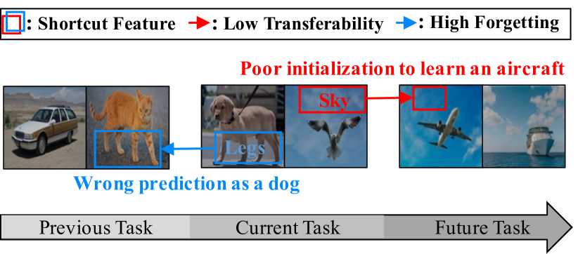
Figure 1: Negative effect of the shortcut bias in OCL: shows the low transferability and high forgetability of shortcut features.

The shortcut bias hinders the main goal of OCL that solves the plasticity and stability dilemma for high transferability and low catastrophic forgetting. That is, it incurs low transferability and high forgetting in OCL, because shortcut features do not generalize well to unseen new classes (Geirhos et al. 2020; Park et al. 2021) and are no longer discriminative for all classes. Figure 1 illustrates the negative effect of the shortcut bias in OCL. Regarding low transferability, if an OCL model learns to use the sky as a shortcut feature for the current task, it is faced with a bad initial point for the future task. Regarding high forgetting, if an OCL model learns to use the dog’s legs for the current task, it is forced to forget the prior knowledge about the legs due to the misclassification of the animals other than the dog.

A significant amount of research has gone into eliminating an undesirable (e.g., shortcut) bias in offline supervised learning. Representative debiasing methods require the prior knowledge of a target task to predefine the undesirable bias for unseen conditions (Bahng et al. 2020; Geirhos et al. 2019; Lee, Kim, and Nam 2019) or leverage auxiliary data such as out-of-distribution (OOD) data (Lee et al. 2021; Park et al. 2021). However, neither prior knowledge nor auxiliary data is available in OCL, because future tasks are inherently unknown and access to auxiliary data is typically constrained due to a limited memory budget. Therefore, overcoming the lack of prior knowledge and auxiliary data should be the main challenge in debiasing for OCL.

Figure 2: Adaptive intensity shifting: shows how the portion of the high-attention features to be dropped can be adjusted in Split ImageNet, where the ground-truth background (shortcut) annotations are available for evaluation.

For shortcut debiasing, we suppress the learning of the shortcut features in a DNN. Accordingly, those shortcut features need to be identified accurately and efficiently without help from prior knowledge and auxiliary data. To this end, we pose two research questions.

RQ1 “Which level of features is the most useful for identifying shortcut features?”: A DNN consists of many layers, and each layer produces its own feature map. Due to the aforementioned uncertainty, we take into account both low-level features from a low-level layer and high-level features from a high-level layer, refining semantic high-level features with structural low-level features via feature map fusion. Our experience indicates that picking up the first and last layers is sufficient for the fusion. Meanwhile, it is known that DNNs prefer to learn shortcut features early owing to their simplicity (Valle-Perez, Camargo, and Louis 2019; Shah et al. 2020; Scimeca et al. 2021), so they tend to have high attention scores. Therefore, we drop the features with top-$\kappa\%$ attention scores on the fused feature map.

RQ2 “How much portion of high-attention features are expected to be shortcut features?”: Answering this question is very challenging because the high-attention features include both shortcut and non-shortcut features, though shortcut features are expected to be dominating. Nevertheless, we endeavor to propose a novel, practical solution called adaptive intensity shifting. In Figure 3, if the features with top-$\kappa\%$ attention scores include a large number of shortcut (e.g., background) features, it is better to increase $\kappa$ to drop shortcut features aggressively (see the 1st histogram); for the opposite case possibly resulted from effective debiasing, it is better to decrease $\kappa$ not to drop useful features (see the 3rd histogram).

Although the idea is very intuitive, there is no ground-truth for shortcut features in practice. Instead, we examine the loss reduction followed by two shift directions—increment and decrement. A bigger loss reduction can be accomplished if more of shortcut features are dropped. The benefit of this loss-based approach is that estimating the dominance of shortcut features in high-attention features does not require additional overhead.

Overall, answering the two questions, we develop a novel framework, DropTop, for suppressing shortcut features in OCL. It is model-agnostic and thus can be incorporated into any replay-based OCL method; two widely-used backbones, a convolutional neural network (CNN) (He et al. 2016) and a Transformer (Dosovitskiy et al. 2021), are adopted for the evaluation. The main contributions of the paper are summarized as follows:

• To the best of our knowledge, this is the first work to address the shortcut bias in OCL. Moreover, we theoretically analyze its negative effect in OCL.

• We present feature map fusion and adaptive intensity shifting to get around the uncertainty caused by the absence of prior knowledge and auxiliary data.

• We empirically show that DropTop improves the average accuracy and forgetting of seven representative OCL methods by up to 10.4% and 63.2%, respectively, on conventional benchmarks as well as newly-introduced benchmarks, namely Split ImageNet-OnlyFG and Split ImageNet-Stylized.

Related Work

Online Continual Learning

Recent studies have mainly considered an online environment for more practical applications (Rolnick et al. 2019; Buzzega et al. 2020; Prabhu, Torr, and Dokania 2020; Bang et al. 2021; Koh et al. 2022; Chaudhry et al. 2018; Kirkpatrick et al. 2017). Access to the data from the current task is permitted until model convergence in an offline environment, but only once in an online environment. Thus, online continual learning (OCL) is much more challenging than offline continual learning. Representative OCL methods are mainly categorized into two groups: replay-based strategies exploiting small episodic memory to consolidate the knowledge of old tasks (Rolnick et al. 2019; Buzzega et al. 2020; Prabhu, Torr, and Dokania 2020; Koh et al. 2022) and regularization-based strategies penalizing a model for rapid parameter updates to avoid the forgetting of old tasks (Chaudhry et al. 2018; Kirkpatrick et al. 2017). In general, replay-based approaches outperform regularization-based ones in terms of accuracy and computational efficiency. Thus, we focus on the replay-based approaches in this paper.

Replay-based approaches suggest the policies for keeping more useful instances. ER (Rolnick et al. 2019) and DER++ (Buzzega et al. 2020) propose random sampling and reservoir sampling, respectively. DER++ (Buzzega et al. 2020) additionally utilizes knowledge distillation (Hinton et al. 2015) to better retain previous knowledge. MIR (Aljundi et al. 2019a) selects the samples whose loss increases the most by a preliminary model update. GSS (Aljundi et al. 2019b) chooses the samples diversifying their gradients. Last, ASER (Shim et al. 2021) retrieves the samples that better preserve latent decision boundaries for known classes while learning new classes.

Debiasing Shorcut Features

The negative impact of shortcuts bias has gained a great attention in the deep learning community (Ilyas et al. 2019; Wang et al. 2020). To prevent the overfitting to the shortcuts, several methods pre-define the type of the target shortcut bias. ReBias (Bahng et al. 2020) removes pixel-level local shortcuts using a set of biased predictions from a bias-characterizing model. Stylized-ImageNet (Geirhos et al. 2019) generates texture-debiased examples. SRM (Lee, Kim, and Nam 2019) synthesizes debiased examples via generative modeling. Another direction is to leverage auxiliary OOD data (Lee et al. 2021; Park et al. 2021), which relies on undesirable features found in the OOD data. However, these existing methods are not directly applicable to our environment, because enforcing prior knowledge or auxiliary data violates the philosophy of OCL.

Moreover, the adverse impact of shortcuts is amplified when training data is insufficient (Lee et al. 2021)—as in OCL involved with an online stream of small tasks. Overall, lack of the prerequisite and rich training data calls for a new debiasing method dedicated for OCL.

Preliminary

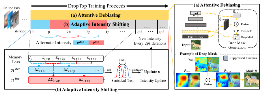
Figure 3: Detailed view of the main components of DropTop: (a) drops the highly-activated features on the fused feature map according to the intensity $\kappa$; as in the example of the drop mask, the fusion facilitates identifying the background shortcuts from the signal of the high-level features on important parts such as the body of the dog. (b) adjusts the drop intensity $\kappa$ for the use in attentive debiasing.

Online Continual Learning

We consider the online continual learning setting, where a sequence of tasks continually emerges with a set of new classes. Each data instance can be accessed only once unless it is stored in episodic memory. For the $t$-th task, let $D_{t}=\{(x^{i}_{t},y^{i}_{t})\}_{i=1}^{m_{t}}$ be a data stream obtained from a joint data distribution over $\mathcal{X}_{t}\times\mathcal{Y}_{t}$, where $\mathcal{X}_{t}$ is the input space, $\mathcal{Y}_{t}$ is the label space in a one-hot fashion, and $m_{t}$ is the number of instances of the $t$-th task. The goal of OCL is to train a classifier, such that it maximizes the test accuracy of all seen tasks $T=\{1,2,\dots,t\}$ at time $t$, with limited or no access to the data stream $D_{t^{\prime}}$ of previous tasks $t^{\prime}<t$.

Shortcut and Non-shortcut Features

Let a DNN model trained on $(x,y)\sim\mathcal{X}\times\mathcal{Y}$ comprises a general feature extractor $f^{\theta}:\mathcal{X}\rightarrow\mathcal{Z}\in\mathbb{R}^{d}$ and a final classifier layer $g^{\text{w}}:\mathcal{Z}\rightarrow\mathbb{R}^{k}$, which is the multiplication of a linear weight matrix $\text{w}\in\mathbb{R}^{k\times d}$ and a feature $z\in\mathcal{Z}$ such that $g^{\text{w}}(z)=w\cdot z$. Here, $k$ is the number of classes, and $d$ is the dimensionality of a feature $z$. Let a feature be the function mapping from the input space $\mathcal{X}$ to a real number; formally speaking, for the $i$-th sub-feature extractor of $f^{\theta}$ where $i\!\in\!\{1,2,\!\ldots\!,d\}$, $f^{\theta}_{i}:\mathcal{X}\rightarrow\mathbb{R}$. DNNs are known to have simplicity bias toward shortcut features which can easily distinguish between given classes (Geirhos et al. 2019; Shah et al. 2020; Geirhos et al. 2020; Pezeshki et al. 2021). Then, the shortcut and non-shortcut features are defined by Definitions 1 and 2, respectively.

Definition 1.

(Shortcut Feature). Let $x$ and $\tilde{x}$ be the instances from seen and unseen data distributions $\mathcal{X}$ and $\mathcal{\tilde{X}}$, respectively, where $\mathcal{X}\cap\mathcal{\tilde{X}}=\emptyset$. We call a feature a shortcut if it is not only highly activated ($\geq\rho$) for the seen data instance but also undesirably activated ($\geq\epsilon$) for the unseen data instance in expectation. That is,

$$f^{\theta}_{s}(\rho,\epsilon):\mathbb{E}_{x\sim\mathcal{X}}\big{[}|f^{\theta}_{s}(x)|\big{]}\geq\rho\leavevmode\nobreak\ \land\leavevmode\nobreak\ \mathbb{E}_{\tilde{x}\sim\mathcal{\tilde{X}}}\big{[}|f^{\theta}_{s}(\tilde{x})|\big{]}\geq\epsilon,\vspace{-0.1cm}$$ (1)

where $s$ is the index of the shortcut feature. $\rho$ and $\epsilon$ are the thresholds indicating high activation for the seen and unseen data distributions.

Note that a shortcut feature, such as an animal’s legs, can be observed from the unseen data instances because it is not an intrinsic feature.

Definition 2.

(Non-shortcut Feature). Let $x$ and $\tilde{x}$ be the instances from seen and unseen data distributions $\mathcal{X}$ and $\mathcal{\tilde{X}}$, respectively, where $\mathcal{X}\cap\mathcal{\tilde{X}}=\emptyset$. We call a feature a non-shortcut if it is highly activated only for the seen instance in expectation. That is,

$$f^{\theta}_{n}(\rho,\epsilon):\mathbb{E}_{x\sim\mathcal{X}}\big{[}|f^{\theta}_{n}(x)|\big{]}\geq\rho\leavevmode\nobreak\ \land\leavevmode\nobreak\ \mathbb{E}_{\tilde{x}\sim\mathcal{\tilde{X}}}\big{[}|f^{\theta}_{n}(\tilde{x})|\big{]}<\epsilon.\vspace{-0.1cm}$$ (2)

Property of Shortcut Feature

Due to a DNN’s simplicity bias, the shortcut features tend to have higher activation values than the non-shortcut features (Shah et al. 2020; Pezeshki et al. 2021), such that

$$\mathbb{E}_{s\in\mathcal{S}}\big{[}|f^{\theta}_{s}(x)|\big{]}>\mathbb{E}_{n\in\mathcal{N}}\big{[}|f^{\theta}_{n}(x)|\big{]},\vspace{-0.1cm}$$ (3)

where $\mathcal{S}$ and $\mathcal{N}$ are the set of the indices of shortcut and non-shortcut features, respectively.

Proposed Method: DropTop

DropTop realizes adaptive feature suppression thorough (a) attentive debiasing with feature map fusion and (b) adaptive intensity shifting. The former drops high-attention features which are expected to be shortcuts, following the guidance from the latter in the form an adjusted drop intensity. Figure 3 illustrates the detailed procedure of DropTop. While (a) attentive debiasing is executed during the learning process, the drop intensity $\kappa$ is periodically adjusted by (b) adaptive intensity shifting. DropTop can be implemented on top of any replay-based OCL methods, and see the implementation detail in Appendix A.

Attentive Debiasing

The shortcut features generally exhibit higher attention scores than the non-shortcut feature by Eq. (3). This shortcut bias usually appears as local or background cues (Scimeca et al. 2021). Thus, after fusing the feature maps of different levels, we generate a drop mask to debias the effect of local or background cues on the feature activation.

Feature Map Fusion

The high-level features are essential to obtain discriminative signals, but they lack fine-grained details (Zhong, Ling, and Wang 2019; Wei et al. 2021), e.g., boundaries of objects. The low-level features embrace structural information with more details, which is helpful for accurately finding shortcut regions as empirically shown in Section Ablation Study. Thus, feature map fusion facilitates the reduction of the ambiguity in identifying the shortcut regions. Specifically, as shown in Figure 3(a), given a small memory footprint, we fuse the feature maps ${F}_{first}\in\mathbb{R}^{h\times w\times c}$ and ${F}_{last}$ $\in\mathbb{R}^{h^{\prime}\times w^{\prime}\times c^{\prime}}$ respectively from the first and last layers. To cope with different resolutions, i.e., $\langle{h,w,c}\rangle\neq\langle{h^{\prime},w^{\prime},c^{\prime}}\rangle$, the last layer’s feature map $F_{last}$ is up-sampled to have the same resolution as the first layer’s feature map $F_{first}$ such that $h^{\prime}=h$ and $w^{\prime}=w$. Then, we conduct average pooling along the channel dimension, compressing the outputs of all $c$ channels to produce the attention map ${A}_{fuse}$, which is derived by

$$\begin{gathered}{F}_{fuse}={F}_{first}\odot{\rm Upsample}({F}_{last})\in\mathbb{R}^{h\times w\times c}\leavevmode\nobreak\ \leavevmode\nobreak\ \text{and}\\ {A}_{fuse}={\rm ChannelPool}(F_{fuse})\in\mathbb{R}^{h\times w},\end{gathered}\vspace*{-0.1cm}$$ (4)

where ChannelPool($\cdot$) is the pooling along the channel, and $\odot$ is the element-wise tensor product.

Drop Mask Generation

Given a drop intensity $\kappa\%$ for each class, we generate a drop mask $M\in\mathbb{R}^{h\times w}$ based on the attention map ${A}_{fuse}$ in Eq. (4). The mask at $(i,j)$ in $M$ is determined by

$$M_{i,j}=\begin{cases}0&\text{if}\!\!\quad(i,j)\in{\rm top\text{-}}\kappa(A_{fuse})\\ 1&\text{otherwise},\\ \end{cases}\vspace*{-0.15cm}$$ (5)

where ${\rm top\text{-}}\kappa(A_{fuse})$ returns the set of the top-$\kappa\%$ elements of $A_{fuse}$. While this hard drop mask is simple and effective, we also test a soft drop mask with continuous values in Appendix E. Last, we apply the drop mask to the first feature map ${F}_{first}$ after the stem layer of a backbone network, e.g., a ResNet or a Vision Transformer (ViT),

$$\tilde{F}_{first}=M\odot{F}_{first}.$$ (6)

This masking process affects all succeeding layers along the forward process. The masked feature map $\tilde{F}_{first}$ accomplishes debiasing by using only the attention scores which can be computed on the fly.

Adaptive Intensity Shifting

The extent of the shortcut bias naturally varies depending on the incoming tasks and the learning progress of a DNN model. Thus, adaptive intensity shifting aims to guide attentive debiasing by adaptively adjusting the drop intensity $\kappa$ in a timely manner. The drop intensity is maintained separately for each class to capture diverse sensitivity to shortcut bias. (See Appendix E for an additional test of sharing the drop intensity across classes.) It is decreased if the removal of features is expected to lose important non-shortcut features which have high predictive power, increased if the removal of features is expected to help emphasize important non-shortcut features, and unchanged in neither of the cases,

$$\kappa\leftarrow\begin{cases}\kappa^{\prime}*\alpha&\text{if decrement}\\ \kappa^{\prime}*(1/\alpha)&\text{if increment}\\ \kappa^{\prime}&\text{otherwise},\end{cases}\vspace*{-0.15cm}$$ (7)

where $\kappa^{\prime}$ is the preceding value, and $\alpha$ $(<1.0)$ is a hyperparameter that indicates the shift step.

Loss Collection

To classify each case, we focus on the contribution to the reduction of the training loss because a better choice of the drop intensity leads to a better training performance (Scimeca et al. 2021; Geirhos et al. 2020). To determine whether a decrement or an increment is preferable, two potential values $\kappa=\kappa^{\prime}*\alpha$ and $\kappa=\kappa^{\prime}*(1/\alpha)$ alternate every $p$ iterations. $p$ is set to be long enough to observe stable behavior with respect to each $\kappa$ option, as shown in Appendix D. The loss reductions are computed at the end of every $p$ iterations and maintained in the set $\mathcal{H}^{dec}$ when $\kappa^{\prime}*\alpha$ is used and in the set $\mathcal{H}^{inc}$ when $\kappa^{\prime}*(1/\alpha)$ is used, as shown in Figure 3(b),

$$\begin{gathered}\,\,\,{\mathcal{H}}^{dec}=\{\Delta\mathcal{L}_{0},\Delta\mathcal{L}_{2p},\dots,\Delta\mathcal{L}_{2p(l-1)}\}\text{and}\\ {\mathcal{H}}^{inc}=\{\underbrace{\Delta\mathcal{L}_{p},\Delta\mathcal{L}_{3p},\dots,\Delta\mathcal{L}_{2pl}}_{\text{Collect }\Delta\mathcal{L}\text{ every }2p\text{ iterations}}\},\end{gathered}\vspace*{-0.1cm}$$ (8)

where $\Delta\mathcal{L}_{(q+1)\cdot p}=\mathcal{L}_{q\cdot p}-\mathcal{L}_{(q+1)\cdot p}$, and $\mathcal{L}_{(q+1)\cdot p}$ is the expected cross-entropy loss on the samples of a specific class in the memory buffer at the iteration $(q+1)\cdot p$. Note that we compute the loss using the samples in the memory buffer rather than in a batch to obtain a more generalizable training loss. Those loss reductions are recorded until ${\mathcal{H}}^{dec}$ and ${\mathcal{H}}^{inc}$ have $l$ elements. Only a single model is needed to compare two shift directions, preserving the memory constraint of OCL; the validity of using a single model is empirically confirmed in Section Evaluation.

Statistical Test and Update

When ${\mathcal{H}}^{dec}$ and ${\mathcal{H}}^{inc}$ become full every $2\cdot p\cdot l$ iterations, we conduct $t$-test to evaluate if the difference between the two directions in the loss reduction is statistically significant, i.e., either $p$-value $\leq 0.05$ or $p$-value $\geq 0.95$. If a better direction exists, the preceding value is updated to the better direction; otherwise, it remains the same. Appendix A describes the pseudocode of adaptive intensity shifting, which is self-explanatory.

Training Data Stabilization

Furthermore, we consider the side effect of shifting the drop intensity during training. If it changes over time, the distribution of input features could be swayed inconsistently. As widely claimed in Ioffe and Szegedy; Zhou et al., this problem often causes training instability and eventually deteriorates the overall performance. In this sense, we decide to drop $\gamma\%$ of the features constantly. Thus, $\kappa$ cannot grow beyond $\gamma$; if $\kappa<\gamma$, $(\gamma-\kappa)$% of the features are additionally chosen uniformly at random among those whose drop mask is not $1$.

Understanding of Shortcut Bias in OCL

From a theoretical standpoint, we clarify two detrimental effects of learning shortcut features in OCL. See Appendix B for relevant empirical evidences. Let $g^{\text{w}}_{i}:\mathbb{R}\rightarrow\mathbb{R}^{k}$ be the multiplication of an $i$-th column vector of the weight matrix w and an $i$-th feature $f_{i}^{\theta}$. Then, $g^{\text{w}}_{i}(f^{\theta}_{i}(x))$ denotes the contribution of the $i$-th feature to a prediction, i.e., how much the $i$-th feature $f^{\theta}_{i}(x)$ contributes to the prediction $g^{\text{w}}(f^{\theta}(x))$, since $g^{\text{w}}(f^{\theta}(x))=\sum_{i=1}^{d}{g^{\text{w}}_{i}(f^{\theta}_{i}(x))}$.

Property 1 (Low Transferability).

A shortcut feature of the current task hinders the model from learning the knowledge of the next task.

Proof.

Let’s consider training a classifier for the ($t$+1)-th task, given a shortcut biased model $\theta_{t}$ as the initial model. By Eq. (1), $\mathbb{E}_{x_{t+1}\sim\mathcal{X}_{t+1}}\big{[}|f^{\theta_{t}}_{s}(x_{t+1})|\big{]}\geq\epsilon$ if $x_{t+1}$ shares the same shortcut features with $x_{t}$. Then, when training a new model $\theta_{t+1}$ from the model $\theta_{t}$, the shortcut feature $f^{\theta_{t}}_{s}$ is no longer discriminative since it can appear in both $\mathcal{X}_{t}$ and $\mathcal{X}_{t+1}$. Thus, the model $\theta_{t+1}$ should learn a totally new discriminative feature, starting from a poor initialization. As a result, the training convergence becomes slower compared with a non-biased model $\theta_{t}^{*}$. $\blacksquare$

Property 2 (High Forgetability).

A shortcut feature of the current task makes the model forget the knowledge of the previous tasks.

Proof.

Given the previous tasks at $t^{\prime}\in\{1,\ldots,t-1\}$ and the current task at $t$, let’s assume that we trained a shortcut biased model $\theta_{t}$. Then, the shortcut feature $s$ of $f^{\theta_{t}}$ contributes to predict the class $y_{t}\in\mathcal{Y}_{t}$ such that $\operatornamewithlimits{argmax}g^{\text{w}_{t}}_{s}(f^{\theta_{t}}_{s}(x_{t}))=y_{t}\in\mathcal{Y}_{t}$. However, by Eq. (1), $\mathbb{E}_{x_{t^{\prime}}\sim\mathcal{X}_{t^{\prime}}}\big{[}|f^{\theta_{t}}_{s}(x_{t^{\prime}})|\big{]}\geq\epsilon$ if $x_{t^{\prime}}$ shares the same shortcut features with $x_{t}$. Then, even for the previous instance $x_{t^{\prime}}$, the shortcut feature $s$ contributes to predict the class $y_{t}\in\mathcal{Y}_{t}$ such that $\operatornamewithlimits{argmax}g^{\text{w}_{t}}_{s}(f^{\theta_{t}}_{s}(x_{t^{\prime}}))=y_{t}\notin\mathcal{Y}_{t^{\prime}}$, which is a wrong prediction. Due to the high activation of shortcut features in Eq. (3), this wrong feature contribution gives a significant impact to the final prediction $g^{\text{w}}(f^{\theta}(x_{t^{\prime}}))=\sum_{i=1}^{d}{g^{\text{w}}_{i}(f^{\theta}_{i}(x_{t^{\prime}}))}$, so that the model highly forgets the knowledge of the previous tasks. $\blacksquare$

Evaluation

Experiment Setting

Dataset Preparation

We validate the debiasing efficacy of DropTop on biased and unbiased setups. A biased setup measures the OCL performance on biased test datasets, where the test dataset shares the same distribution of shortcut features with the training dataset, e.g., the sky background in the bird class. On the other hand, an unbiased setup (Bahng et al. 2020) does not contain the shortcut features in the test dataset, so that we can more clearly measure the debiasing efficacy.

Biased Setup: We use the Split CIFAR-10 (Krizhevsky, Hinton et al. 2009), Split CIFAR-100 (Krizhevsky, Hinton et al. 2009), and Split ImageNet-9 (Xiao et al. 2020) for the biased setup. Split CIFAR-10 and Split CIFAR-100 consist of five different tasks with non-overlapping classes, and thus each task contains two and 20 classes, respectively. The details of Split ImageNet-9 are provided in Appendix C.

Unbiased Setup: The evaluation of unbiased setup is conducted after being trained on Split ImageNet-9. We introduce two Split ImageNet-9 variants: Split ImageNet-OnlyFG and Split ImageNet-Stylized, which are generated by debiasing two realistic shortcuts, the background and the local texture cue, respectively. In ImageNet-OnlyFG (Xiao et al. 2020), the background is removed to evaluate the dependecy on the background in image recognition; in ImageNet-Stylized (Geirhos et al. 2019), the local texture is shifted by style-transfer, and the reliance of a model on the local texture cue is removed. Performance improvements on these two datasets indicate that DropTop helps untie undesirable dependency on the realistic shortcuts.

Algorithms and Evaluation Metrics

We apply DropTop to seven popular algorithms including ER (Rolnick et al. 2019) and DER++ (Buzzega et al. 2020), MIR (Aljundi et al. 2019a), GSS (Aljundi et al. 2019b), ASER (Shim et al. 2021), L2P (Wang et al. 2022b), and DualPrompt (Wang et al. 2022a). They are all actively being cited. The experimental details are presented in Appendix E. We adopt widely-used performance measures (Aljundi et al. 2019b; Shim et al. 2021; Koh et al. 2022): (1) average accuracy $A_{avg}=\frac{1}{T}\Sigma_{i=1}^{T}A_{i}$, where $A_{i}$ is the accuracy at the end of the $i$-th task, and (2) forgetting $F_{last}=\frac{1}{T-1}\Sigma_{j=1}^{T-1}f_{T,j}$, where $f_{i,j}$ indicates how much the model forgets about the $j$-th task after learning the $i$-th task ($j<i$). For reliability, we repeat every experiment five times with different random seeds and report the average value with the standard error. We report the relative improvements (denoted as “Rel. Improv.”) by DropTop for each metric. All algorithms are implemented using PyTorch 1.12.1 and tested on a single NVIDIA RTX 2080Ti GPU, and the source code is available at https://github.com/kaist-dmlab/DropTop.

	Biased Setup						Unbiased Setup
	Split CIFAR-100		Split CIFAR-10		Split ImageNet-9		Split ImageNet-OnlyFG		Split ImageNet-Stylized
Method	$A_{avg}$ ($\uparrow$)	$F_{last}$ ($\downarrow$)	$A_{avg}$ ($\uparrow$)	$F_{last}$ ($\downarrow$)	$A_{avg}$ ($\uparrow$)	$F_{last}$ ($\downarrow$)	$A_{avg}$ ($\uparrow$)	$F_{last}$ ($\downarrow$)	$A_{avg}$ ($\uparrow$)	$F_{last}$ ($\downarrow$)
ER	25.3 ($\pm$0.2)	19.2 ($\pm$0.3)	55.4 ($\pm$0.3)	39.9 ($\pm$2.4)	46.1 ($\pm$0.2)	55.8 ($\pm$1.8)	32.8 ($\pm$0.4)	45.0 ($\pm$1.5)	39.3 ($\pm$0.3)	49.7 ($\pm$0.9)
$+$DropTop	26.5 ($\pm$0.2)	18.3 ($\pm$1.3)	61.0 ($\pm$0.6)	37.6 ($\pm$1.9)	48.9 ($\pm$0.4)	44.0 ($\pm$3.8)	35.9 ($\pm$0.9)	47.8 ($\pm$3.7)	41.3 ($\pm$0.1)	38.9 ($\pm$2.6)
1-11   Rel. Improv.	4.4%	4.9%	10.2%	5.7%	6.1%	21.1%	9.4%	-6.2%	5.1%	21.8%
DER++	23.6 ($\pm$0.3)	33.4 ($\pm$0.7)	59.8 ($\pm$0.8)	28.2 ($\pm$1.5)	44.2 ($\pm$1.0)	63.0 ($\pm$4.6)	33.2 ($\pm$0.5)	61.6 ($\pm$2.1)	37.8 ($\pm$0.7)	60.3 ($\pm$3.2)
$+$DropTop	25.1 ($\pm$0.3)	31.1 ($\pm$1.2)	62.6 ($\pm$0.7)	23.7 ($\pm$1.0)	45.4 ($\pm$0.5)	60.7 ($\pm$5.1)	34.5 ($\pm$0.7)	54.9 ($\pm$3.2)	39.7 ($\pm$0.4)	58.9 ($\pm$4.1)
1-11   Rel. Improv.	6.4%	6.9%	4.7%	16.0%	2.8%	3.6%	3.7%	11.0%	4.9%	2.4%
MIR	20.8 ($\pm$0.6)	25.3 ($\pm$1.7)	51.5 ($\pm$0.5)	58.4 ($\pm$1.3)	39.3 ($\pm$1.2)	41.1 ($\pm$2.0)	32.1 ($\pm$0.4)	38.9 ($\pm$3.1)	34.0 ($\pm$1.0)	40.7 ($\pm$1.6)
$+$DropTop	22.4 ($\pm$0.1)	24.8 ($\pm$1.0)	51.6 ($\pm$0.6)	56.3 ($\pm$1.6)	42.0 ($\pm$0.9)	39.3 ($\pm$4.5)	35.4 ($\pm$1.4)	36.0 ($\pm$3.1)	36.1 ($\pm$0.6)	38.3 ($\pm$3.4)
1-11   Rel. Improv.	8.1%	1.9%	0.2%	3.7%	6.8%	4.4%	10.4%	7.5%	6.0%	6.0%
GSS	21.8 ($\pm$0.3)	27.9 ($\pm$0.8)	46.0 ($\pm$0.4)	69.7 ($\pm$0.7)	40.3 ($\pm$0.6)	71.5 ($\pm$2.0)	34.5 ($\pm$0.9)	65.6 ($\pm$0.7)	35.3 ($\pm$0.7)	64.2 ($\pm$1.9)
$+$DropTop	23.7 ($\pm$0.2)	28.4 ($\pm$1.0)	49.1 ($\pm$0.5)	69.2 ($\pm$1.5)	41.3 ($\pm$0.6)	68.5 ($\pm$1.9)	36.5 ($\pm$0.7)	61.6 ($\pm$1.8)	35.9 ($\pm$0.4)	62.3 ($\pm$2.3)
1-11   Rel. Improv.	8.8%	-1.7%	6.5%	0.6%	2.3%	4.2%	5.9%	6.1%	1.8%	2.9%
ASER	32.7 ($\pm$0.1)	41.8 ($\pm$0.4)	50.3 ($\pm$0.5)	57.8 ($\pm$3.3)	39.7 ($\pm$0.7)	62.6 ($\pm$2.1)	30.2 ($\pm$0.2)	60.2 ($\pm$0.9)	33.6 ($\pm$0.5)	56.8 ($\pm$1.1)
$+$DropTop	33.4 ($\pm$0.4)	39.5 ($\pm$0.8)	51.3 ($\pm$0.3)	57.5 ($\pm$0.8)	41.6 ($\pm$0.8)	57.5 ($\pm$3.2)	31.2 ($\pm$0.2)	49.6 ($\pm$2.8)	35.5 ($\pm$0.4)	52.6 ($\pm$2.5)
1-11   Rel. Improv.	2.3%	5.3%	2.0%	0.4%	4.8%	8.2%	3.4%	17.7%	5.7%	7.3%

Table 1: Average accuracy (higher is better) and forgetting (lower is better) on Split CIFAR-100, Split CIFAR-10, and Split ImageNet-9 for a biased setup and on Split ImageNet-OnlyFG and Split ImageNet-Stylized for an unbiased setup. The best values are marked in bold.

Improvements through Debiasing

Biased Setup

Table 1 summarizes the performance of five replay-based OCL methods with and without applying DropTop under the biased and unbiased setups. Overall, DropTop consistently improves their performances with respect to $A_{avg}$ and $F_{last}$. Quantitatively, $A_{avg}$ and $F_{last}$ are improved by 5.3% and 6.5%, respectively, on average across all baselines and datasets. That is, the debiasing by DropTop is very effective in OCL regardless of the method and dataset. In addition, the high $A_{avg}$ and the low $F_{last}$ demonstrate that the proposed debiasing approach helps expedite the training convergence of OCL models (higher transferability) and retain the knowledge of the previous tasks well (lower forgetability).

In detail, the effect of our method is the most prominent for ER, increasing $A_{avg}$ by 7.0% on average. In particular, DropTop improves the performances of ER and DER++ on Split CIFAR-10 and Split CIFAR-10 by 10.2% and 9.4% in terms of $A_{avg}$ and by 5.7% and 16.0% in terms of $F_{last}$, respectively. In contrast, ASER is improved relatively less. Since ASER is designed for keeping the samples with high diversity in the memory, we conjecture that the adverse effect of shortcut features is naturally smaller than random sampling as in ER and DER++.

	Split ImageNet-9		ImageNet-OnlyFG		ImageNet-Stylized
​​​​​​​​​​​​​​​​Method​​​​​​​​​​​​​	$A_{avg}$ ($\uparrow$)	$F_{last}$ ($\downarrow$)	$A_{avg}$ ($\uparrow$)	$F_{last}$ ($\downarrow$)	$A_{avg}$ ($\uparrow$)	$F_{last}$ ($\downarrow$)
L2P​​​	95.3 ($\pm$0.7)	12.6 ($\pm$1.9)	91.0 ($\pm$0.7)	20.6 ($\pm$2.2)	87.7 ($\pm$0.5)	25.8 ($\pm$1.8)
$+$DropTop​​​	97.1 ($\pm$0.4)	5.6 ($\pm$1.1)	92.9 ($\pm$0.4)	12.7 ($\pm$0.6)	89.7 ($\pm$0.8)	18.3 ($\pm$1.0)
1-7 Rel. Improv.​​​​​	1.9%	55.4%	2.1%	38.3%	2.3%	28.9%
DualPrompt​​​	96.1 ($\pm$0.6)	9.9 ($\pm$1.4)	90.8 ($\pm$1.2)	20.0 ($\pm$2.0)	86.3 ($\pm$1.5)	29.2 ($\pm$2.4)
$+$DropTop​​​	97.5 ($\pm$0.3)	3.7 ($\pm$0.8)	93.5 ($\pm$0.5)	9.8 ($\pm$0.5)	89.9 ($\pm$0.6)	16.6 ($\pm$0.8)
1-7 Rel. Improv.​​​​​	1.5%	63.2%	2.9%	51.0%	4.2%	43.1%

Table 2: Performance of DropTop on top of pretrained ViT-based CL algorithms, L2P and DualPrompt, on Split ImageNet-9, Split ImageNet-OnlyFG, and Split ImageNet-Stylized.

Unbiased Setup

The improvement of DropTop becomes more noticeable in the unbiased setup than in the biased setup, because this unbiased setup does not contain the shortcut features in the test datasets. For example, in Table 1, the relative improvement for MIR on Split ImageNet-OnlyFG is $10.4\%$, while that on Split ImageNet-9 is $6.8\%$. In addition, DropTop is more effective in reducing the background bias than the local cue bias; $A_{avg}$ improves by $6.6\%$ on average for all methods in Split ImageNet-OnlyFG, which is larger than $4.7\%$ in Split ImageNet-Stylized. Achieving high accuracy for the unbiased setup requires robustly generalizing to more intrinsic complex features beyond less generalizable shortcut features. Obviously, attentive debiasing coordinated by adaptive intensity shifting supports the requirement by suppressing the undesirable reliance on shortcut features.

Debiasing Pretrained ViT-based CL

We test DropTop’s adaptability to a pretrained ViT since it has been used frequently in recent CL studies, by injecting DropTop into L2P and DualPrompt in an online setting. Table 2 shows the performance of L2P and DualPrompt with and without DropTop on the Split ImageNet datasets. We note that both versions of L2P or DualPrompt are modified to perform experience replay (Rolnick et al. 2019) using the small replay buffer for a fair comparison. Overall, DropTop consistently exhibits significant improvements in both forgetting and accuracy, where the accuracy is initially high due to pretraining. Quantitatively, $F_{last}$ and $A_{avg}$ are improved by 46.7% and 2.5%, respectively, on average across the datasets and algorithms. This result clearly demonstrates the universal need for mitigating the shortcut bias in different backbone networks as well as DropTop’s excellent adaptability. Please see Appendix F for the result on more datasets.

		No Drop Int. Shift
Method	No MF	Rand Drop	Fixed Drop	DropTop
ER	43.8	43.9	44.1	45.5
DER++	42.0	41.6	43.4	44.4
MIR	38.0	37.8	39.3	38.7
GSS	34.7	34.8	37.0	38.0
ASER	40.5	41.4	40.5	42.1
AVG (Degrad.)	39.8 (-4.9%)	39.9 (-4.5%)	40.9 (-2.1%)	41.7

Table 3: Ablation study on multi-level feature fusion and drop intensity shifting with respect to the accuracy $A_{avg}$ averaged over the biased datasets: Split CIFAR-100, Split CIFAR-10, and Split ImageNet-9. The highest values are marked in bold.

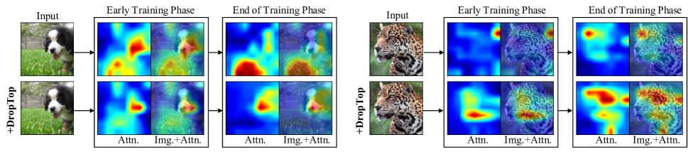
(a) Debiasing the background shortcut bias.                                 (b) Debiasing the local cue bias.

Figure 4: Visualization of the gradual debiasing process by DropTop. The results are the activation maps from ER and ER$+$DropTop trained on Split ImageNet-9: (a) and (b) are respectively related to debiasing the background and local cue bias during training, where the bias is the reliance on the grass background in (a) and on a local part of a leopard (e.g., part of the face without the body) in (b).

Ablation Study

We conduct an ablation study to examine the general effectiveness of multi-level feature fusion in Eq. (4) and adaptive intensity shifting in Eq. (7). Table 3 compares DropTop with its three variants with respect to the average accuracy across the biased datasets (Split CIFAR-100, Split CIFAR-10, and Split ImageNet-9). The results for the unbiased datasets are presented in Appendix E. No MF drops only high-level features without multi-level fusion, Rand Drop drops randomly chosen features, and Fixed Drop drops the features with the highest attention scores without adaptive intensity shifting.

Multi-level Feature Fusion

The first variant, No MF, omits multi-level feature fusion for generating the drop masks, which solely relies on the high-level features. As a result, it shows the worst average accuracy among the variants. In particular, compared to DropTop which relies on the first and last layers for multi-level feature fusion, the average accuracy drops significantly by 4.9% on average. Therefore, refining semantic high-level features with structural low-level features via feature map fusion is essential to precisely identify the shortcut features.

Adaptive Intensity Shifting

The other two variants, Rand Drop and Fixed Drop, do not apply adaptive intensity shifting while dropping the same proportion of the features as DropTop. Based on their accuracy worse than DropTop, we conclude that drop intensity shifting makes further improvements. Quantitatively, without drop intensity shifting, they face the average degradation of 4.5% and 2.1% compared with the complete DropTop. Therefore, adaptively adjusting the drop intensity is needed for effective debiasing to catch the continuously varying proportion of the shortcut features in a timely manner. Furthermore, the superior performance of DropTop as well as Fixed Drop over Rand Drop verifies that debiasing based on highly activated features cannot be easily replaced by the regularization effect of the random drop (Srivastava et al. 2014).

Qualitative Analysis for Debiasing Effect

Figure 4 visualizes the activation maps of ER with and without DropTop on Split ImageNet-9 to qualitatively analyze the debiasing effect. In summary, we observe that DropTop gradually alleviates the shortcut bias as the training proceeds whereas the original ER increasingly relies on the shortcut bias—the background and local cue. In Figure 4(a) for the background bias, as the training proceeds, ER$+$DropTop successfully debiases the grass background and, eventually, focuses on the intrinsic shapes of the dog at the end of training whereas ER rather intensifies the reliance on the background. In Figure 4(b) for the local cue bias, ER$+$DropTop gradually expands the extent of the discriminative regions to cover the overall shapes of the object, resulting in more accurate and comprehensive recognition of the leopard compared with ER. Please see Appendix H for more visualizations.

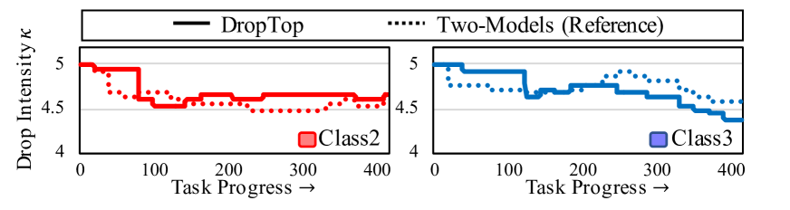
Figure 5: Comparison between the original and two-model versions of DropTop regarding the adjustments of the drop intensity $\kappa$ for Split CIFAR-10 on top of ER.

Validity of Drop Intensity Adjustments

One might think that alternating the increment and decrement of $\kappa$ with a single model is invalid because the effect of one option may influence that of the other option. Using only a single model is inevitable because of the memory restriction in OCL, as discussed in Section Adaptive Intensity Shifting. Thus, by assuring the period for each option to be long enough, we aim to reducing undesirable influence between the two options. To verify the validity of our approach, we implement a two-model “reference” version that maintains two separate models, each for increment and decrement, but does violate the memory restriction. As shown in Figure 5, the original version adjusts $\kappa$ very similarly to the reference version. Quantitatively, 82.1$\pm$0.6% of the adjustments of $\kappa$ coincide with each other, and their accuracy is nearly identical, 61.0$\pm$0.6% and 61.5$\pm$0.2% for the test.

Conclusion

We propose a debiasing OCL method called DropTop, introducing two novel solutions for debiasing shortcut features, attentive debiasing with feature map fusion and adaptive intensity shifting. Without relying on prior knowledge and auxiliary data, DropTop determines the appropriate level and proportion of possible short features and drops them from the feature map for debiasing. It can easily be built on top of any existing replay-based OCL methods. The evaluation confirms that DropTop significantly improves the existing state-of-the-art OCL methods. Overall, we believe that our work sheds the light on the importance of debiasing shortcuts in OCL.

A  Pseudocode of DropTop

Algorithm 1 Replay-based OCL with DropTop

0:  Number of tasks $T$, online data stream $\{D_{1},\dots,D_{T}\}$, total drop ratio $\gamma$, softmax function $\sigma$, learning rate $\eta$, batch size $b$

0:  Model parameters $\theta,w$ after learning task $T$

1:  $\theta,w\leftarrow\text{Initialize model parameters};$

2:  $\mathcal{B}\leftarrow\text{Initialize replay memory};$

3:  $\kappa\leftarrow\text{Initialize class-wise debiasing intensity};$

4:  for $t=1$ to $T$ do

5:     for $i=1$ to $|D_{t}|/b$ do

6:        ${X}_{n},{Y}_{n}$ $\leftarrow$ a mini-batch from online data stream $D_{t}$;

7:        /* Replay Memory Retrieval */

8:        ${X}_{m},{Y}_{m}$ $\leftarrow$ ${\rm MemoryRetrieve}(\mathcal{B},{X}_{n},{Y}_{n})$;

9:        /* Attentive Debiasing in Sec. 4.1 */

10:        $M$ $\leftarrow$ ${\rm MultiLevelDropMask}({X}_{n}\cup{X}_{m};\theta,\kappa,\gamma)$;

11:        $P$ $\leftarrow$ $\sigma({\rm DebiasForward}({X}_{n}\cup{X}_{m},M;\theta,w))$;

12:        /* Model Update */

13:        Compute the loss $\mathcal{J}$ using ${Y}_{n}\cup{Y}_{m}$ and ${P}$;

14:        $\theta\leftarrow\theta-\eta\nabla_{\theta}\mathcal{J}$;  $w\leftarrow w-\eta\nabla_{w}\mathcal{J}$;

15:        /* Replay Memory Update */

16:        $\mathcal{B}$ $\leftarrow$ ${\rm MemoryUpdate}(\mathcal{B},{X}_{n},{Y}_{n})$;

17:        /* Adaptive Intensity Shifting in Sec. 4.2 */

18:        $\kappa$ $\leftarrow$ ${\rm AdjustDropIntensity}(\mathcal{M},i)$;

19:     end for

20:  end for

21:  return  $\theta,w$;

Algorithm 1 describes how DropTop works with replay-based online continual learning (OCL) methods. Various replay-based algorithms are applied by using their respective methods for MemoryRetrieve (Line 8) and MemoryUpdate (Line 15). At the beginning, a model and a memory buffer are initialized for a replay-based algorithm; and class-wise drop intensity is initialized for our DropTop (Lines 1–3). The model receives two minibatches from the online data stream and the memory buffer, respectively (Lines 6–8). The forward propagation is carried out through the online debiasing layer (Lines 9–11). First, a drop mask is obtained by masking top $\kappa$% and random $(\gamma-\kappa)$% of the multi-level features (Line 10). Next, the drop mask is applied to the forward pass by multiplying it element-by-element with the intermediate feature maps (Line 11). Then, based on the cross-entropy loss with the combined batch, the backward propagation is carried out to update the model parameters (Lines 12–14). In addition, the replay algorithm performs an online update of the memory buffer using the minibatch from the data stream (Lines 15–16). Last, the class-wise drop intensity for each class is updated (Lines 17–18). The detailed pseudocode of adaptive intensity shifting is described in Algorithm 2, which is self-explanatory.

Algorithm 2 Adaptive Intensity Shifting

0:  Preceding intensity: $\kappa^{\prime}$, step size: $\alpha$, alternating period: $p$, episodic memory of each class: $\mathcal{B}$, model parameters: $\{\theta,w\}$, training iteration: $i$

0:  Drop intensity $\kappa$ that will be applied to the next model update

1:  /* Initialize candidate strategies */

2:  $\kappa^{dec}\leftarrow\kappa^{\prime}*\alpha;\leavevmode\nobreak\ \leavevmode\nobreak\ \kappa^{inc}\leftarrow\kappa^{\prime}*(1/\alpha);$

3:  {$\mathcal{H}^{dec},\mathcal{H}^{inc}\}\leftarrow{\rm InitializeHistory}()$;

4:  if ${\rm mod}(i,p)=0$ then

5:     /* Compute contribution of intensity */

6:     $\mathcal{L}_{new}$ $\leftarrow$ ${\rm Loss}(\mathcal{B},\{\theta,w\})$;

7:     $\Delta\mathcal{L}\leftarrow\mathcal{L}_{old}-\mathcal{L}_{new}$;

8:      ${\rm UpdateHistory}(\{\mathcal{H}^{dec},\mathcal{H}^{inc}\},\Delta\mathcal{L})$;

9:     $\mathcal{L}_{old}$ $\leftarrow$ $\mathcal{L}_{new}$;

10:     /* Update Intensity based on Statistical Test */

11:     if ${\rm full}(\mathcal{H}^{dec},\mathcal{H}^{inc})$ then

12:        if ${\rm\textit{p}\text{-}value}(\mathcal{H}^{dec},\mathcal{H}^{inc})\leq 0.05$ then

13:           $\kappa^{inc}$ $\leftarrow$ $\kappa^{dec}$;

14:           $\kappa^{dec}$ $\leftarrow$ $\kappa^{dec}*\alpha$;

15:        else if ${\rm\textit{p}\text{-}value}(\mathcal{H}^{dec},\mathcal{H}^{inc})\geq 0.95$ then

16:           $\kappa^{dec}$ $\leftarrow$ $\kappa^{inc}$;

17:           $\kappa^{inc}$ $\leftarrow$ $\kappa^{inc}*(1/\alpha)$;

18:        end if

19:        ${\rm ResetHistory}(\mathcal{H}^{dec},\mathcal{H}^{inc})$;

20:     end if

21:     /* Alternate two shift directions  */

22:     $\kappa\leftarrow{\rm AlternateBetween}(\kappa^{dec},\kappa^{inc},i)$ ;

23:  else

24:     $\kappa\leftarrow\kappa^{\prime}$;

25:  end if

26:  return  $\kappa$;

B  Empirical Proofs of Low Transferability and High Forgetting

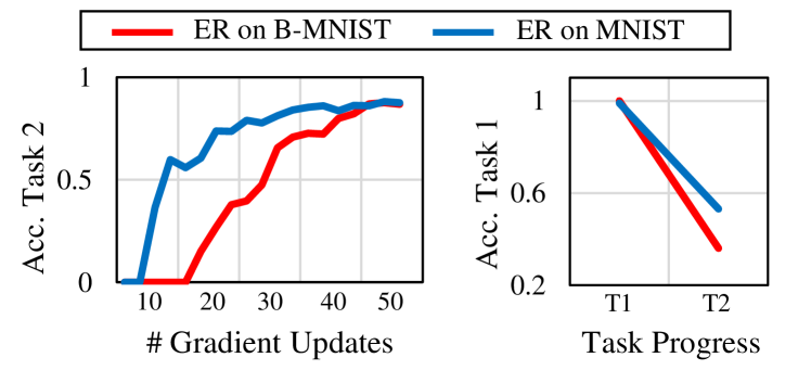
(a) Transferability.             (b) Forgetability.

Figure 6: Shortcut learning in OCL: (a) shows lower transferability from Task 1 (0 and 1) to Task 2 (2 and 3), and (b) shows high forgetting of Task 1 (0 and 1) by Task 2 (2 and 3), compared with non-shortcut learning.

To empirically investigate transferability and forgetting, we conduct a simple controlled experiment using Biased MNIST (B-MNIST) (Bahng et al. 2020), which is a widely-used dataset in bias learning (Bahng et al. 2020; Bui et al. 2021; Tartaglione, Barbano, and Grangetto 2021), as well as MNIST (LeCun et al. 1998). In B-MNIST, each digit is in a different color, e.g., 0 in red and 1 in green. DNNs trained on B-MNIST employ only color shortcut features for classification because the color is a simpler feature than the shape of a digit. We train ER (Rolnick et al. 2019) for OCL with two tasks—Task 1 (T1) classifying 0 and 1, and Task 2 (T2) classifying 2 and 3.

Low Transferability. Figure 6(a) shows that shortcut features have lower transferability than non-shortcut features. When training T2, ER trained on B-MNIST (the shortcut-biased model) shows slower increase of test accuracy than ER trained on MNIST, since the red and green color features learned in T1 are not applicable to T2. This result indicates that the transferability of the OCL model significantly deteriorates once the model is biased towards the shortcut features.

High Forgetability. Figure 6(b) shows that shortcut features have higher forgetting than non-shortcut features. After training T2, ER trained on B-MNIST shows rapid forgetting of the prediction capability in T1, since the red or green color becomes a shortcut cue to predict the digit 2 or 3 in T2. This result indicates that the OCL model is also significantly damaged by forgetting once the model is biased towards the shortcut features.

	OCL						Standard
​​​​​​​​​​​​​​​​Dataset​​​​​​​​​​​​​	$Task_{1}$	$Task_{2}$	$Task_{3}$	$Task_{4}$	$A_{avg}$ ($\uparrow$)​​	$F_{last}$ ($\downarrow$)​​	$Acc.$ ($\uparrow$)
OnlyBG​	54.4 $\pm$2.2	35.4 $\pm$1.7	21.6 $\pm$1.6	16.3 $\pm$0.8 ​​​​	31.9 $\pm$1.2 ​​	45.6 $\pm$1.7 ​​​​​​​	28.4 $\pm$1.6
OnlyFG​	54.0 $\pm$0.3	37.3 $\pm$2.3	24.9 $\pm$0.6	21.2 $\pm$0.6 ​​​​	34.4 $\pm$0.6 ​​	40.5 $\pm$1.6 ​​​​​​​	29.1 $\pm$0.4
1-8 Rel. Improv.​​​	-0.8%	5.5%	15.4%	29.6%	7.6%	11.1%	2.7%

Table 4: Impact of shortcut bias on OCL and standard learning.

Impact of Realistic Shortcuts on OCL. Table 4 compares the performance of DNNs in OCL and standard learning with and without background shortcut features. In longer OCL with real-world images, the shortcut bias on background significantly degrades the performance. Moreover, the negative impact of the shortcut bias is much more pronounced in OCL than in standard learning. In detail, to enable or disable the shortcut bias, ER was trained using two ImageNet-variant datasets (Xiao et al. 2020): OnlyBackground (OnlyBG) and OnlyForeground (OnlyFG). ER trained on OnlyBG experienced a more severe degradation in terms of accuracy (transferability) and forgetting, by 7.6% and 11.1% respectively, compared with ER trained on OnlyFG. In standard learning, the accuracy gap between two datasets is much smaller at 2.7%.

C  Split ImageNet-9 Datasets

ImageNet-9 (Xiao et al. 2020), a subset of ImageNet (Deng et al. 2009), contains 9 coarser-level classes: Dog, Bird, Vehicle, Reptile, Carnivore, Insect, Instrument, Primate, and Fish. Additionally, the ratio of the classes is balanced, and each class has about 4,500 instances. See Appendix A of (Xiao et al. 2020) for the further details of ImageNet-9.

Task Configuration. Split ImageNet-9 is constructed for the continual learning environment by evenly distributing the 9 classes into 4 tasks except the class Primate. Thus, the 4 sequential tasks are (Dog, Bird), (Vehicle, Reptile), (Carnivore, Insect), and (Instrument, Fish).

Split ImageNet-9 Variants for the Unbiased Setup. The two variants are used to measure the debiasing efficacy of DropTop. Split ImageNet-OnlyFG is created by adopting the same split of ImageNet as originally done in (Xiao et al. 2020). Similarly, Split ImageNet-Stylized is created by applying the same split of Stylized ImageNet as done in (Geirhos et al. 2019).

D  Hyperparameter Sensitivity Analysis

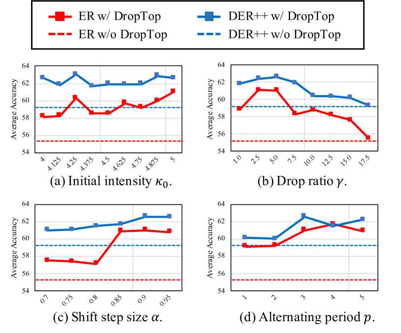
Figure 7: Parameter sensitivity analysis: the default values are the initial drop intensity $\kappa_{0}=5.0$%, the drop ratio $\gamma=5.0$%, the shifting step size $\alpha=0.9$, and the alternating period $p=3$. Each subfigure shows how the average accuracy $A_{avg}$ of five runs changes as only one of the hyperparamters varies.

The hyperparameters of DropTop are the initial drop intensity $\kappa_{0}$, the total drop ratio $\gamma$, the shifting step size $\alpha$, and the alternating period $p$. Figure 7 shows how each hyperparameter affects the average accuracy with ER (Rolnick et al. 2019) and DER (Buzzega et al. 2020).

Initial Drop Intensity. The initial drop intensity $\kappa_{0}$ is continuously shifted during the training period coordinated by adaptive intensity shifting. Figure 7(a) shows that the performance is consistently high over a wide range of $\kappa_{0}$, and we conjecture that the continuous adjustment of the intensity leads to such consistency. Among similarly good values, we set $\kappa_{0}=5.0$% at which ER and DER++ peak, for all experiments of these algorithms. The values of the hyperparameters for the other algorithms are chosen in the same way.

Drop Ratio. A proper drop ratio $\gamma$ prevents too much removal of informative features and too small debiasing effect. Interestingly, Figure 7(b) shows that the performance begins to drop if $\gamma$ is greater than $7.5$% while losing the benefit from DropTop if $\gamma$ becomes $17.5$%; thus, we set $\gamma=5.0$% as the proper drop ratio for all experiments.

Shifting Step Size. The shifting step size $\alpha$ determines the size of a single intensity update to handle the varying extent of the shortcut bias. The smaller $\alpha$, the larger a shifting step size. Figure 7(c) shows that DropTop achieves consistently high performance as long as $\alpha$ is greater than 0.85, and particularly we set $\alpha=0.9$ where the performance peaks, for all experiments. For a small $\alpha$ (a large shifting step size), the drop intensity may not be finely adjusted, resulting in suboptimal performances.

Alternating Period. The alternating period $p$ decides how often the contribution of each intensity to the loss reduction is measured. If two intensities alternate too often with a small $p$, measuring the contribution of the intensity will become inconsistent and inaccurate. In this sense, we observe consistently high performances when $p$ is greater than or equal to 3, as in Figure 7(d). Therefore, $p$ is decided to 3 for all experiments.

E  Complete Experiment Results

Implementation Settings

For all algorithms and datasets, the size of a minibatch from the data stream and the replay memory is set to 32 (Buzzega et al. 2020). The size of episodic memory is set to 500 for Split CIFAR-10 and Split ImageNet-9 and 2,000 for Split CIFAR-100 depending on the total number of classes. In order to add DropTop’s debiasing capability to L2P and DualPrompt, which are originally rehearsal-free, we attach small replay memory whose size is reduced to 200 and 500, respectively. We train ResNet18 using SGD with a learning rate of 0.1 (Buzzega et al. 2020; Shim et al. 2021) for all ResNet-based algorithms. We optimize L2P and DualPrompt with a pretrained ViT-B/16 using Adam with a learning rate of 0.05, $\beta_{1}$ of 0.9, and $\beta_{2}$ of 0.999.

Since we follow the widely-used OCL setting of (Shim et al. 2021; Buzzega et al. 2020) regarding the batch sizes, optimizer, backbone, etc., we adopt the hyperparameter values selected through an extensive grid search in the same OCL setting (Shim et al. 2021; Buzzega et al. 2020). Specifically, we adopt the values of ER and DER++ following (Buzzega et al. 2020), those of MIR, GSS, and ASER following (Shim et al. 2021), and those of L2P and DualPrompt following (Wang et al. 2022a).

The hyperparameters specific to the individual algorithms are set for all datasets as follows:

• ER (Rolnick et al. 2019): No additional hyperparameters.

• DER++ (Buzzega et al. 2020): The coefficient of knowledge distillation loss is set to 0.2, and the coefficient of the cross entropy loss using a batch from the memory buffer is set to 0.5.

• MIR (Aljundi et al. 2019a): The number of subsamples for searching maximally interfered samples is set to 50.

• GSS (Aljundi et al. 2019b): The number of batches from the memory buffer to estimate the maximal similarity score is set to 10.

• ASER (Shim et al. 2021): The mean values of Adversarial SV and Cooperative SV are used as a type of ASER. The number of samples per class is set to 1.5, and the number of neighbors for computing KNN-SV is set to 3.

• L2P (Wang et al. 2022b): The prompt length, top-N, and size of the prompt pool are set to 5, 5, and 10, respectively. Besides, to provide an optimization similar to DualPrompt (Wang et al. 2022a), we apply prefix tuning-based prompts to the first through fifth Transformer layers.

• DualPrompt (Wang et al. 2022a): The general prompts with a length of 5 are applied to the first and second Transformer layers, while the expert prompts with a length of 20 are applied to the third, fourth, and fifth Transformer layers.

For the empirical proofs in Appendix B, we use ER with the ResNet18 backbone and SGD with an initial learning rate of 0.001. The size of episodic memory is set to 200.

Hyperparameters

There are a few hyperparameters introduced by DropTop. For attentive debiasing, we fix the total drop ratio $\gamma$ to $5.0\%$ and set the initial drop intensity $\kappa_{0}$ to $5.0\%$ for ER, DER++, and MIR and to $0.5\%$ for GSS and ASER, differently depending on the sampling method. For L2P and DualPrompt, we set $\gamma$ and $\kappa_{0}$ to $2.0\%$ and $1.0\%$, respectively, owing to the difference of the backbone network. For adaptive intensity shifting, we fix the history length $l$ to $10$, which is approximately the minimum sample size for one-sided $t$-test with the significance level 0.05 (Heckert et al. 2002). The alternating period $p=3$ and the shifting step size $\alpha=0.9$ are adequate across the algorithms and datasets. Please see Appendix D for the sensitivity analysis of the hyperparameters and Appendix E for the hyperparameter tuning (Buzzega et al. 2020) for the other algorithms.

Method	$A_{avg}$ ($\uparrow$)	Degrade	$F_{last}$ ($\downarrow$)	Degrade
Soft Drop Mask	60.3 ($\pm$0.4)	1.1%	40.4 ($\pm$3.1)	7.4%
Common Drop Intensity	57.6 ($\pm$0.1)	5.6%	42.7 ($\pm$1.6)	13.6%
DropTop	61.0 ($\pm$0.6)	—	37.6 ($\pm$1.9)	—

Table 5: Performance of ER+DropTop with alternative design choices: the soft drop mask for attentive debiasing (Section 4.1) and a common drop intensity for all classes (Section 4.2).

Considerations of Alternative Design Choices

Soft Drop Mask for Attentive Debiasing. We test a soft drop mask by replacing the hard drop mask in Eq. (5). Specifically, the soft drop mask linearly reduces the dependence on a shortcut feature as its attention value increases. That is, the soft drop mask at $(i,j)$ in a drop mask $M$ is determined by

$$M_{i,j}=\begin{cases}\frac{{\rm rank\text{-}}\kappa(i,j)}{|{\rm top\text{-}}\kappa(A_{fuse})|}&\text{if}\!\!\quad(i,j)\in{\rm top\text{-}}\kappa(A_{fuse})\\ 1&\text{otherwise},\\ \end{cases}\vspace*{-0.15cm}$$ (9)

where ${\rm top\text{-}}\kappa(A_{fuse})$ returns the set of the top-$\kappa\%$ elements of $A_{fuse}$ and ${\rm rank\text{-}}\kappa(i,j)$ returns the rank of the value at $(i,j)$ within ${\rm top\text{-}}\kappa(A_{fuse})$ in descending order. Table 5 shows a slight degradation by the soft drop mask, meaning that it is more effective to lessen reliance on shortcut features by outright excluding them.

Common Drop Intensity for All Classes. We test a common drop intensity shared across classes by replacing class-wise drop intensities that capture diverse sensitivities of classes to shortcut features. Using a single common drop intensity notably degrades performance by 5.6% and 13.6% in terms of average accuracy and forgetting, as shown in Table 5. This result provides clear evidence for the necessity of maintaining class-wise drop intensities.

Ablation Studies for Unbiased Setup

Table 6 compares DropTop with its three variants across the unbiased datasets, Split ImageNet-OnlyFG and Split ImageNet-Stylized, where a sharper degradation of the performance indicates a stronger dependence on shortcut features. In general, the results for the unbiased datasets are consistent with those for the biased datasets.

		No Drop Int. Shift
Method	No MF	Rand Drop	Fixed Drop	DropTop
ER	35.2	38.1	39.1	39.4
DER++	34.0	33.7	38.0	37.1
MIR	33.1	32.3	36.6	35.8
GSS	33.4	32.2	32.4	36.2
ASER	33.0	31.7	33.1	33.4
AVG (Degrad.)	33.7 (-7.9%)	33.6 (-8.3%)	35.8 (-1.6%)	36.4

Table 6: Ablation study on multi-level feature fusion and drop intensity shifting with respect to the accuracy $A_{avg}$ averaged over the unbiased datasets: Split ImageNet-OnlyFG and Split ImageNet-Stylized. The highest values are marked in bold.

Multi-level Feature Fusion. The first variant, No MF, drops only high-level features without multi-level fusion. Compared with the results of the biased datasets, the degradation by No MF on the unbiased datasets is sharper from the degradation of 4.9% to 7.9%, meaning that the multi-level fusion reduces undesirable bias towards shortcuts. Therefore, the multi-level fusion is essential to precisely capture shortcut features.

	GPU Memory (GB)	Running Time (mins.)
ER	4.509	42.55
ER+DropTop	4.563 (+0.054 / 1.183%)	49.26 (+6.71 / 13.62%)

Table 7: Computational overhead incurred by DropTop.

Adaptive Intensity Shifting. Rand Drop drops randomly chosen features, and Fixed Drop drops the features with the highest attention scores, where neither of them uses adaptive intensity shifting. As a result, we consistently observe that using adaptive intensity shifting makes further improvements over the two variants by 8.3% and 1.6%. In particular, Rand Drop becomes the worst for the unbiased setup, emphasizing that random drop-based regularization is not suitable for debiasing the shortcut features.

Computational Complexity

Table 7 reports the GPU memory and OCL time of ER with and without DropTop on Split ImageNet-9, showing that DropTop efficiently debiases shortcuts. The additional cost of DropTop is only $\frac{p+1}{p}$ forward passes on average per iteration, where $p$ is the alternating period ($p\!=\!3$ in the paper); it is much smaller than the total cost of ER (especially including backward passes). A forward pass is inexpensive, costing roughly one-third as much as a backward pass (Li et al. 2020).

	Split CIFAR-100			Split CIFAR-10
Method	$A_{last}$ ($\uparrow$)	$A_{avg}$ ($\uparrow$)	$F_{last}$ ($\downarrow$)	$A_{last}$ ($\uparrow$)	$A_{avg}$ ($\uparrow$)	$F_{last}$ ($\downarrow$)
L2P​​​	72.3 ($\pm$0.6)	81.5 ($\pm$1.2)	24.3 ($\pm$0.9)	85.8 ($\pm$1.1)	92.2 ($\pm$1.3)	16.6 ($\pm$1.4)
$+$DropTop​​​	74.3 ($\pm$0.7)	82.1 ($\pm$0.6)	21.9 ($\pm$1.1)	89.3 ($\pm$0.7)	94.0 ($\pm$0.2)	12.2 ($\pm$0.8)
1-8   Rel. Improv.​​​	2.7%	0.7%	9.9%	4.0%	1.9%	26.7%
DualPrompt​​​	73.5 ($\pm$0.5)	83.2 ($\pm$0.8)	22.5 ($\pm$0.8)	89.5 ($\pm$1.6)	94.9 ($\pm$1.3)	11.8 ($\pm$0.7)
$+$DropTop​​​	74.0 ($\pm$0.4)	82.7 ($\pm$0.4)	21.5 ($\pm$0.6)	90.5 ($\pm$0.4)	95.0 ($\pm$0.2)	10.5 ($\pm$0.5)
1-8   Rel. Improv.​​​	0.7%	-0.6%	4.5%	1.2%	0.1%	11.2%

Table 8: Performance of DropTop on top of pretrained ViT-based CL algorithms, L2P (Wang et al. 2022b) and DualPrompt (Wang et al. 2022a), on Split CIFAR-100, and Split CIFAR-10. The highest values are marked in bold.

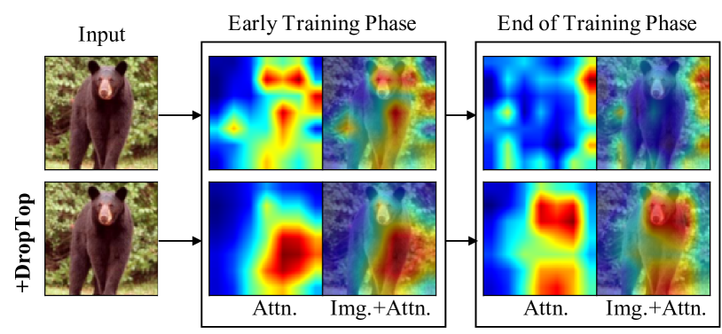
(a) Debiasing the background shortcut bias.

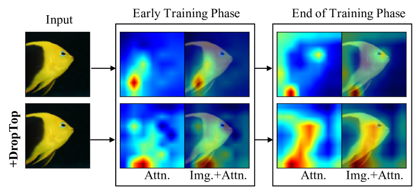
(b) Debiasing the local cue bias.

Figure 8: Additional visualization of the gradual debiasing process by DropTop. The results are the activation maps from ER and ER$+$DropTop trained on Split ImageNet-9: (a) and (b) are respectively related to debiasing the background and local cue bias during training, where the bias is the reliance on the grass background in (a) and on a local part of a fish (e.g., its eye without the body) in (b).

F  Debiasing Pretrained ViT-based CL

In addition to Table 2, Table 8 shows the performance of L2P (Wang et al. 2022b) and DualPrompt (Wang et al. 2022a) with and without DropTop on Split CIFAR-100 and Split CIFAR-10 in an online setting. Overall, the results for the CIFAR datasets are consistent with those for the ImageNet datasets. Specifically, DropTop improves $F_{last}$, $A_{last}$, and $A_{avg}$ by 13.1%, 2.2%, and 0.5%, respectively, on average across the datasets and algorithms. The relatively modest improvement observed in $A_{avg}$ can be attributed to the slow convergence of the prompt tuning mechanism, which has been widely acknowledged (Huang et al. 2022; Su et al. 2022), in L2P and DualPrompt. This slow convergence leads to a gradually increasing dependence on shortcut features, which reduces the effectiveness of debiasing in the early stages of training. Consequently, the improvement observed in $A_{avg}$ becomes less significant than that observed in $A_{last}$. Nevertheless, the overall improvements by DropTop again emphasize the compelling need for mitigating the shortcut bias, irrespective of backbone networks.

G  Limitations and Future Work

DropTop has consistently improved performance on a range of datasets when combined with different OCL algorithms. However, it is necessary to formally formulate the effectiveness of DropTop in light of the characteristics of datasets and OCL algorithms. Although debiasing shortcut features by DropTop is effective since DNNs are highly susceptible to the shortcut bias (Shah et al. 2020), as shown in Section Evaluation, its effectiveness varies by OCL algorithms and datasets. Therefore, determining the effectiveness of debiasing shortcuts based on such characteristics would be an interesting research area.

H  Additional Visualization of Debiasing

Last, in addition to Figure 4, we present another visualization in Figure 8 which was omitted owing to lack of space. Again, Figure 8 verifies that DropTop gradually alleviates the shortcut bias as the training proceeds whereas the original ER increasingly relies on the shortcut bias—the background and local cue.

References

- Aljundi et al. (2019a) Aljundi, R.; Belilovsky, E.; Tuytelaars, T.; Charlin, L.; Caccia, M.; Lin, M.; and Page-Caccia, L. 2019a. Online Continual Learning with Maximal Interfered Retrieval. In NeurIPS, 11849–11860.
- Aljundi et al. (2019b) Aljundi, R.; Lin, M.; Goujaud, B.; and Bengio, Y. 2019b. Gradient Based Sample Selection for Online Continual Learning. In NeurIPS.
- Bahng et al. (2020) Bahng, H.; Chun, S.; Yun, S.; Choo, J.; and Oh, S. J. 2020. Learning De-biased Representations with Biased Representations. In ICML, 528–539.
- Bang et al. (2021) Bang, J.; Kim, H.; Yoo, Y.; Ha, J.-W.; and Choi, J. 2021. Rainbow Memory: Continual Learning with a Memory of Diverse Samples. In CVPR, 8218–8227.
- Bui et al. (2021) Bui, M.-H.; Tran, T.; Tran, A.; and Phung, D. 2021. Exploiting Domain-specific Features to Enhance Domain Generalization. NeurIPS, 21189–21201.
- Buzzega et al. (2020) Buzzega, P.; Boschini, M.; Porrello, A.; Abati, D.; and Calderara, S. 2020. Dark Experience for General Continual Learning: a Strong, Simple Baseline. NeurIPS, 15920–15930.
- Chaudhry et al. (2018) Chaudhry, A.; Dokania, P. K.; Ajanthan, T.; and Torr, P. H. 2018. Riemannian Walk for Incremental Learning: Understanding Forgetting and Intransigence. In ECCV, 532–547.
- De Lange et al. (2021) De Lange, M.; Aljundi, R.; Masana, M.; Parisot, S.; Jia, X.; Leonardis, A.; Slabaugh, G.; and Tuytelaars, T. 2021. A Continual Learning Survey: Defying Forgetting in Classification Tasks. IEEE Transactions on Pattern Analysis and Machine Intelligence, 44(7): 3366–3385.
- Deng et al. (2009) Deng, J.; Dong, W.; Socher, R.; Li, L.-J.; Li, K.; and Fei-Fei, L. 2009. Imagenet: A Large-scale Hierarchical Image Database. In 2009 IEEE conference on computer vision and pattern recognition, 248–255. IEEE.
- Dosovitskiy et al. (2021) Dosovitskiy, A.; Beyer, L.; Kolesnikov, A.; Weissenborn, D.; Zhai, X.; Unterthiner, T.; Dehghani, M.; Minderer, M.; Heigold, G.; Gelly, S.; Uszkoreit, J.; and Houlsby, N. 2021. An Image is Worth 16x16 Words: Transformers for Image Recognition at Scale. In ICLR.
- Du et al. (2021) Du, M.; Manjunatha, V.; Jain, R.; Deshpande, R.; Dernoncourt, F.; Gu, J.; Sun, T.; and Hu, X. 2021. Towards Interpreting and Mitigating Shortcut Learning Behavior of NLU Models. arXiv preprint arXiv:2103.06922.
- Geirhos et al. (2020) Geirhos, R.; Jacobsen, J.-H.; Michaelis, C.; Zemel, R.; Brendel, W.; Bethge, M.; and Wichmann, F. A. 2020. Shortcut Learning in Deep Neural Networks. Nature Machine Intelligence, 2(11): 665–673.
- Geirhos et al. (2019) Geirhos, R.; Rubisch, P.; Michaelis, C.; Bethge, M.; Wichmann, F. A.; and Brendel, W. 2019. ImageNet-trained CNNs Are Biased Towards Texture; Increasing Shape Bias Improves Accuracy and Robustness. In ICLR.
- He et al. (2016) He, K.; Zhang, X.; Ren, S.; and Sun, J. 2016. Deep Residual Learning for Image Recognition. In CVPR, 770–778.
- Heckert et al. (2002) Heckert, N. A.; Filliben, J. J.; Croarkin, C. M.; Hembree, B.; Guthrie, W. F.; Tobias, P.; Prinz, J.; et al. 2002. Handbook 151: NIST/SEMATECH e-handbook of Statistical Methods. NIST Interagency/Internal Report (NISTIR).
- Hendrycks et al. (2021) Hendrycks, D.; Zhao, K.; Basart, S.; Steinhardt, J.; and Song, D. 2021. Natural Adversarial Examples. In CVPR, 15262–15271.
- Hinton et al. (2015) Hinton, G.; Vinyals, O.; Dean, J.; et al. 2015. Distilling the Knowledge in a Neural Network. arXiv preprint arXiv:1503.02531.
- Huang et al. (2022) Huang, Y.; Qin, Y.; Wang, H.; Yin, Y.; Sun, M.; Liu, Z.; and Liu, Q. 2022. FPT: Improving Prompt Tuning Efficiency via Progressive Training. In EMNLP, 6877–6887.
- Ilyas et al. (2019) Ilyas, A.; Santurkar, S.; Tsipras, D.; Engstrom, L.; Tran, B.; and Madry, A. 2019. Adversarial Examples are Not Bugs, They are Features. In NeurIPS.
- Ioffe and Szegedy (2015) Ioffe, S.; and Szegedy, C. 2015. Batch Normalization: Accelerating Deep Network Training by Reducing Internal Covariate Shift. In ICML, 448–456. PMLR.
- Kirkpatrick et al. (2017) Kirkpatrick, J.; Pascanu, R.; Rabinowitz, N.; Veness, J.; Desjardins, G.; Rusu, A. A.; Milan, K.; Quan, J.; Ramalho, T.; Grabska-Barwinska, A.; et al. 2017. Overcoming Catastrophic Forgetting in Neural Networks. Proceedings of the National Academy of Sciences, 114(13): 3521–3526.
- Koh et al. (2022) Koh, H.; Kim, D.; Ha, J.-W.; and Choi, J. 2022. Online Continual Learning on Class Incremental Blurry Task Configuration with Anytime Inference. In ICLR.
- Krizhevsky, Hinton et al. (2009) Krizhevsky, A.; Hinton, G.; et al. 2009. Learning Multiple Layers of Features from Tiny Images. Technical Report.
- LeCun et al. (1998) LeCun, Y.; Bottou, L.; Bengio, Y.; and Haffner, P. 1998. Gradient-based Learning Applied to Document Recognition. Proceedings of the IEEE, 86: 2278–2324.
- Lee, Kim, and Nam (2019) Lee, H.; Kim, H.-E.; and Nam, H. 2019. Srm: A Style-based Recalibration Module for Convolutional Neural Networks. In ICCV, 1854–1862.
- Lee et al. (2021) Lee, S.; Park, C.; Lee, H.; Yi, J.; Lee, J.; and Yoon, S. 2021. Removing Undesirable Feature Contributions Using Out-of-Distribution Data. In ICLR.
- Li et al. (2020) Li, S.; Zhao, Y.; Varma, R.; Salpekar, O.; Noordhuis, P.; Li, T.; Paszke, A.; Smith, J.; Vaughan, B.; and Damania, P. 2020. PyTorch Distributed: Experiences on Accelerating Data Parallel Training. Proceedings of the VLDB Endowment.
- Park et al. (2021) Park, D.; Song, H.; Kim, M.; and Lee, J.-G. 2021. Task-Agnostic Undesirable Feature Deactivation Using Out-of-Distribution Data. In NeurIPS, 4040–4052.
- Pezeshki et al. (2021) Pezeshki, M.; Kaba, O.; Bengio, Y.; Courville, A. C.; Precup, D.; and Lajoie, G. 2021. Gradient Starvation: A Learning Proclivity in Neural Networks. NeurIPS, 1256–1272.
- Prabhu, Torr, and Dokania (2020) Prabhu, A.; Torr, P. H.; and Dokania, P. K. 2020. Gdumb: A Simple Approach that Questions Our Progress in Continual Learning. In ECCV, 524–540.
- Rolnick et al. (2019) Rolnick, D.; Ahuja, A.; Schwarz, J.; Lillicrap, T.; and Wayne, G. 2019. Experience Replay for Continual Learning. NeurIPS.
- Scimeca et al. (2021) Scimeca, L.; Oh, S. J.; Chun, S.; Poli, M.; and Yun, S. 2021. Which Shortcut Cues Will Dnns Choose? A Study from the Parameter-space Perspective. arXiv preprint arXiv:2110.03095.
- Shah et al. (2020) Shah, H.; Tamuly, K.; Raghunathan, A.; Jain, P.; and Netrapalli, P. 2020. The Pitfalls of Simplicity Bias in Neural Networks. NeurIPS, 9573–9585.
- Shim et al. (2021) Shim, D.; Mai, Z.; Jeong, J.; Sanner, S.; Kim, H.; and Jang, J. 2021. Online Class-Incremental Continual Learning with Adversarial Shapley Value. In AAAI, 9630–9638.
- Srivastava et al. (2014) Srivastava, N.; Hinton, G.; Krizhevsky, A.; Sutskever, I.; and Salakhutdinov, R. 2014. Dropout: A Simple Way to Prevent Neural Networks from Overfitting. The Journal of Machine Learning Research, 15(1): 1929–1958.
- Su et al. (2022) Su, Y.; Wang, X.; Qin, Y.; Chan, C.-M.; Lin, Y.; Wang, H.; Wen, K.; Liu, Z.; Li, P.; Li, J.; et al. 2022. On Transferability of Prompt Tuning for Natural Language Processing. In NAACL, 3949–3969.
- Tartaglione, Barbano, and Grangetto (2021) Tartaglione, E.; Barbano, C. A.; and Grangetto, M. 2021. End: Entangling and Disentangling Deep Representations for Bias Correction. In CVPR, 13508–13517.
- Valle-Perez, Camargo, and Louis (2019) Valle-Perez, G.; Camargo, C. Q.; and Louis, A. A. 2019. Deep Learning Generalizes Because the Parameter-function Map is Biased towards Simple Functions. In ICLR.
- Wang et al. (2020) Wang, H.; Wu, X.; Huang, Z.; and Xing, E. P. 2020. High-frequency Component Helps Explain the Generalization of Convolutional Neural Networks. In CVPR, 8684–8694.
- Wang et al. (2022a) Wang, Z.; Zhang, Z.; Ebrahimi, S.; Sun, R.; Zhang, H.; Lee, C.-Y.; Ren, X.; Su, G.; Perot, V.; Dy, J.; et al. 2022a. Dualprompt: Complementary Prompting for Rehearsal-free Continual Learning. In ECCV, 631–648.
- Wang et al. (2022b) Wang, Z.; Zhang, Z.; Lee, C.-Y.; Zhang, H.; Sun, R.; Ren, X.; Su, G.; Perot, V.; Dy, J.; and Pfister, T. 2022b. Learning to Prompt for Continual Learning. In CVPR, 139–149.
- Wei et al. (2021) Wei, J.; Wang, Q.; Li, Z.; Wang, S.; Zhou, S. K.; and Cui, S. 2021. Shallow Feature Matters for Weakly Supervised Object Localization. In CVPR, 5993–6001.
- Xiao et al. (2020) Xiao, K.; Engstrom, L.; Ilyas, A.; and Madry, A. 2020. Noise or Signal: The Role of Image Backgrounds in Object Recognition. arXiv preprint arXiv:2006.09994.
- Zhong, Ling, and Wang (2019) Zhong, G.; Ling, X.; and Wang, L.-N. 2019. From Shallow Feature Learning to Deep Learning: Benefits from the Width and Depth of Deep Architectures. Wiley Interdisciplinary Reviews: Data Mining and Knowledge Discovery, 9: e1255.
- Zhou et al. (2022) Zhou, S.; Zhao, H.; Zhang, S.; Wang, L.; Chang, H.; Wang, Z.; and Zhu, W. 2022. Online Continual Adaptation with Active Self-Training. In AISTATS, 8852–8883.