Depolarization dyadics for truncated spheres, spheroids, and ellipsoids

Abstract

Depolarization dyadics play a central role in theoretical studies involving scattering from small particles and homogenization of particulate composite materials. Closed-form expressions for depolarization dyadics have been developed for truncated spheres and truncated spheroids, and the formalism has been extended to truncated ellipsoids; the evaluation of depolarization dyadics for this latter case requires numerical integration. The Hölder continuity condition has been exploited to fix the origin of the coordinate system for the evaluation of depolarization dyadics. These results will enable theoretical studies involving scattering from small particles and homogenization of particulate composite materials to accommodate particles with a much wider range of shapes than was the case hitherto.

Keywords: Depolarization dyadic, Hölder continuity, singularity, truncated spheroid, truncated sphere

1 Introduction

The calculation of the electric field due to a specified source current density is a fundamental problem in electromagnetics [1]. The usual approach involves integration of a suitable product of a dyadic Green function and the source current density over the source region (i.e., the region occupied by the source current density) [2, 3]. This process is particularly challenging if the electric field is sought in the source region, since the singularity of dyadic Green function must be considered then [4]. The integrated singularity of the dyadic Green function — known as the depolarization dyadic — is a central pillar in scattering and homogenization theories [5, 6].

The depolarization dyadic is expressible in terms of a surface integral. The evaluation of this integral is crucially dependent upon the shape of the surface. For relatively simple shapes, such as spherical [4], spheroidal [7, 8], ellipsoidal [9, 10, 11, 12], cylindrical [13, 14], cubical [13], and polyhedral [15], closed-form expressions for depolarization dyadics have been developed, but for more complex shapes numerical methods must be used for their evaluation.

In this communication, closed-form expressions are developed for truncated spheres and spheroids, and these are illustrated numerically. The formalism is extended to truncated ellipsoids. Hereafter, $\varepsilon_{\scriptscriptstyle 0}$, $\mu_{\scriptscriptstyle 0}$, and $k_{\scriptscriptstyle 0}=\omega\sqrt{\varepsilon_{\scriptscriptstyle 0}\mu_{\scriptscriptstyle 0}}$ are the free-space permittivity, permeability, and wavenumber, respectively, with $\omega$ being the angular frequency; an $\exp(-i\omega t)$ time-dependence is implicit; and $\underline{\underline{I}}=\hat{{\bf u}}_{\rm x}\hat{{\bf u}}_{\rm x}+\hat{{\bf u}}_{\rm y}\hat{{\bf u}}_{\rm y}+\hat{{\bf u}}_{\rm z}\hat{{\bf u}}_{\rm z}$ is the identity dyadic, with $\hat{{\bf u}}_{\rm x}$, $\hat{{\bf u}}_{\rm y}$, and $\hat{{\bf u}}_{\rm z}$ being unit vectors aligned with the Cartesian coordinate axes .

2 Depolarization dyadics

Suppose that a time-harmonic source current density ${\bf J}({\bf r})$ exists inside a finite region $V_{s}$ which is bounded by a closed surface. The unbounded region outside $V_{s}$ is vacuous. The time-harmonic electric field both outside and inside $V_{s}$ is given as [1]

$${\bf E}({\bf r})=i\omega\mu_{\scriptscriptstyle 0}\int_{V_{s}}\underline{\underline{G}}({\bf r},{\bf r}_{s})\mbox{ \tiny{${}^{\bullet}$} }{\bf J}({\bf r}_{s})\,d^{3}{\bf r}_{s},$$ (1)

wherein

$$\underline{\underline{G}}({\bf r},{\bf r}_{s})=\left(\underline{\underline{I}}+\frac{\nabla\nabla}{k_{\scriptscriptstyle 0}^{2}}\right)\frac{\exp\left(ik_{\scriptscriptstyle 0}|{\bf r}-{\bf r}_{s}|\right)}{4\pi|{\bf r}-{\bf r}_{s}|}$$ (2)

is the free-space dyadic Green function [3].

For field points outside the source region, i.e., ${\bf r}\notin V_{s}$, the integral on the right side of Eq. (1) is well behaved and its evaluation delivers ${\bf E}({\bf r})$ as an analytic function. For field points inside the source region, i.e., ${\bf r}\in V_{s}$, the evaluation of the integral on the right side of Eq. (1) requires care because the dyadic Green function is singular at ${\bf r}={\bf r}_{s}$ [4]. In particular, the double derivative in the free-space dyadic Green function (2) gives rise to a $|{\bf r}-{\bf r}_{s}|^{-3}$ term. This is not integrable unless the source current density ${\bf J}({\bf r})$ satisfies the following Hölder continuity condition: there exist three positive constants $a_{1}$, $a_{2}$, and $a_{3}$ such that [16]

$$|{\bf J}({\bf r})-{\bf J}({\bf r}_{s})|\leq a_{1}|{\bf r}-{\bf r}_{s}|^{a_{2}}$$ (3)

for all ${\bf r}_{s}$ satisfying $|{\bf r}-{\bf r}_{s}|\leq a_{3}$.

Provided that the Hölder continuity condition (3) is satisfied, the electric field inside the source region $V_{s}$ may be expressed as [17]

$${\bf E}({\bf r})=i\omega\mu_{\scriptscriptstyle 0}\lim_{\delta\to 0}\int_{V_{s}-V_{\delta}}\underline{\underline{G}}({\bf r},{\bf r}_{s})\mbox{ \tiny{${}^{\bullet}$} }{\bf J}({\bf r}_{s})\,d^{3}{\bf r}_{s}+\frac{1}{i\omega\varepsilon_{\scriptscriptstyle 0}}\underline{\underline{L}}\mbox{ \tiny{${}^{\bullet}$} }{\bf J}({\bf r}),\qquad{\bf r}\in V_{s}.$$ (4)

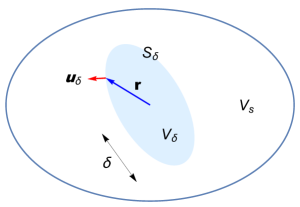
(a) Exclusion region $V_{\delta}$ inside source region $V_{s}$.

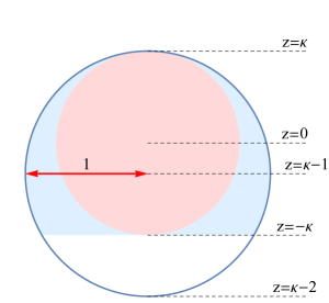
(b) Truncated unit sphere with largest inscribed sphere of radius $\kappa\in(0,1)$.

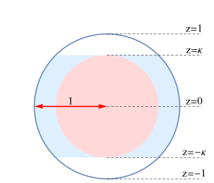
(c) Double-truncated unit sphere with largest inscribed sphere of radius $\kappa\in(0,1)$.

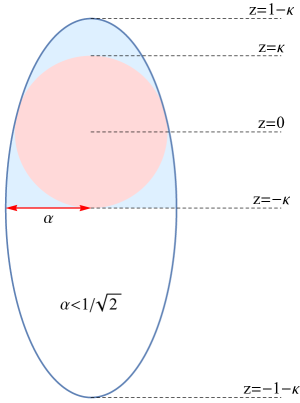
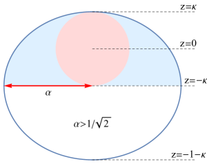
(d) Hemispheroid with largest inscribed sphere of radius $\kappa\in(0,1)$ for $\alpha<1/\sqrt{2}$ (top) and $\alpha>1/\sqrt{2}$ (bottom).

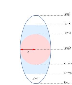
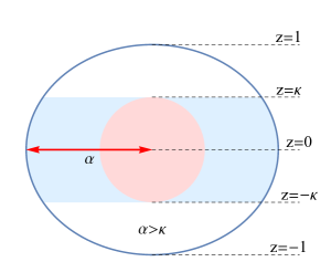
(e) Double-truncated spheroid with largest inscribed sphere of radius $\alpha$ for $\alpha<\kappa$ (top) and of radius $\kappa$ for $\alpha>\kappa$ (bottom).

Figure 1: Schematic representations of exclusion regions.

Herein $V_{\delta}\subset V_{s}$ is an exclusion region of linear dimensions quantifiable through a small length $\delta$, and surface $S_{\delta}$, that contains the singular point ${\bf r}={\bf r}_{s}$; a schematic representation is displayed in Fig. 1(a). The depolarization dyadic

$$\underline{\underline{L}}=\frac{1}{4\pi}\int_{S_{\delta}}\frac{{\bf u}_{\delta}\,{\bf r}}{|{\bf r}|^{3}}\,d^{2}{\bf r},$$ (5)

with ${\bf u}_{\delta}$ being the unit outward normal vector to $S_{\delta}$. The shape of $V_{\delta}$ should be such that ${\bf u}_{\delta}$ is unambiguously identified at every point on $S_{\delta}$, but edges on $S_{\delta}$ can be rounded off slightly to overcome this restriction, if necessary.

The question arises: Where inside the exclusion region $V_{\delta}$ should the coordinate origin be taken for the integration that delivers the depolarization dyadic in Eq. (5)? In the case of the spherical exclusion region, there is no problem because $\underline{\underline{L}}=(1/3)\underline{\underline{I}}$ regardless of where the coordinate origin is located inside $V_{\delta}$ [4]. However, $\underline{\underline{L}}$ generally depends on the choice of coordinate origin for less symmetric exclusion regions [17, 18]. The origin of the coordinate system must therefore be taken as the center of the largest sphere that can be inscribed inside the exclusion region $V_{\delta}$, so that the Hölder continuity condition (3) holds over the largest portion of $V_{\delta}$.

In the following sections, depolarization dyadics are calculated for exclusions regions shaped as truncated spheres, spheroids, and ellipsoids. For a truncated ellipsoid whose principal axes are aligned with the axes of the Cartesian coordinate system, the depolarization dyadic has the diagonal form

$$\underline{\underline{L}}=L_{x}\,\hat{{\bf u}}_{\rm x}\hat{{\bf u}}_{\rm x}+L_{y}\,\hat{{\bf u}}_{\rm y}\hat{{\bf u}}_{\rm y}+L_{z}\,\hat{{\bf u}}_{\rm z}\hat{{\bf u}}_{\rm z};$$ (6)

with $L_{x}=L_{y}\equiv L$ for truncated spheres and truncated spheroids. Furthermore, the trace of the depolarization dyadic

$$\mbox{trace}\left\{\underline{\underline{L}}\right\}=\frac{1}{4\pi}\int_{S_{\delta}}\frac{{\bf u}_{\delta}\mbox{ \tiny{${}^{\bullet}$} }{\bf r}}{|{\bf r}|^{3}}\,d^{2}{\bf r}$$ (7)

represents the normalized solid angle of the surface $S_{\delta}$ as viewed from ${\bf r}={\bf 0}$ [17]. Hence, $\mbox{trace}\left\{\underline{\underline{L}}\right\}=1$. Accordingly, in the following presentation of closed-form expressions for depolarization dyadics for truncated spheres and spheroids, there is no need to provide explicit expressions for $L_{z}$ because $L_{z}=1-2L$.

3 Spherical geometry

3.1 Truncated sphere

Suppose that the unit sphere centered at $x=y=0,z=\kappa-1$, i.e.,

$$x^{2}+y^{2}+\left(z-\kappa+1\right)^{2}\leq 1,$$ (8)

is bifurcated by the plane $z=-\kappa$, where $0<\kappa<1$, as schematically illustrated in Fig. 1(b). The exclusion region $V_{\delta}$ is the upper part of the sphere bounded below by the plane $z=-\kappa$, and the largest inscribed sphere is specified by

$$x^{2}+y^{2}+z^{2}\leq\kappa^{2}.$$ (9)

After integrating over both the curved and the flat parts of $S_{\delta}$, we found from Eq. (5) that $\underline{\underline{L}}=L\left(\hat{{\bf u}}_{\rm x}\hat{{\bf u}}_{\rm x}+\hat{{\bf u}}_{\rm y}\hat{{\bf u}}_{\rm y}\right)+L_{z}\,\hat{{\bf u}}_{\rm z}\hat{{\bf u}}_{\rm z}$ with

$$L=\frac{\kappa}{6\left(1-\kappa\right)^{3}\tau}\,\left\{6-\tau\left(3-3\kappa+\kappa^{2}\right)-\kappa\left[11-3\kappa\left(3-\kappa\right)\right]\right\},$$ (10)

where

$$\tau=\sqrt{\left(4-3\kappa\right)\kappa};$$ (11)

and confirmed that $L_{z}=1-2L$. Observe that $L\to 0$ and $L_{z}\to 1$ in the limit $\kappa\to 0$, while $L\to 1/3$ and $L_{z}\to 1/3$ in the limit $\kappa\to 1$, in agreement with well-known results [4].

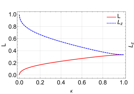
Figure 2: $L$ and $L_{z}$ plotted against $\kappa\in(0,1)$ for the truncated unit sphere.

Plots of the depolarization factors $L$ and $L_{z}$ versus $\kappa$ are provided in Fig. 2. As $\kappa$ increases, the value of $L$ increases monotonically whereas the value of $L_{z}$ decreases monotonically. For all $\kappa<1$, $L_{z}>L$. The case of the hemisphere, i.e., $\kappa=1/2$, for which $L=(19/6\sqrt{5})-7/6=0.24951$ and $L_{z}=\left(50-19\sqrt{5}\right)/15=0.500981$ is notable: $L_{z}$ is approximately – but not exactly – equal to $2L$.

3.2 Double-truncated sphere

Suppose that the unit sphere centered at the origin of the coordinate system, i.e.,

$$x^{2}+y^{2}+z^{2}\leq 1,$$ (12)

is symmetrically trifurcated by the planes $z=-\kappa$ and plane $z=\kappa$, where $0<\kappa<1$, per the schematic representation in Fig. 1(c). The exclusion region $V_{\delta}$ is the double-truncated sphere bounded by the planes $z=\pm\kappa$.

The depolarization dyadic for this $V_{\delta}$ again is of the form $\underline{\underline{L}}=L\left(\hat{{\bf u}}_{\rm x}\hat{{\bf u}}_{\rm x}+\hat{{\bf u}}_{\rm y}\hat{{\bf u}}_{\rm y}\right)+L_{z}\,\hat{{\bf u}}_{\rm z}\hat{{\bf u}}_{\rm z}$. With the largest inscribed sphere specified by Eq. (9), we determined

$$L=\frac{\left(3-\kappa^{2}\right)\kappa}{6}$$ (13)

from Eq. (5) and verified that $L_{z}=1-2L$.

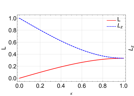
Figure 3: $L$ and $L_{z}$ plotted against $\kappa\in(0,1)$ for the double-truncated unit sphere.

In Fig. 3, the depolarization factors $L$ and $L_{z}$ are plotted against $\kappa$. As is the case for the truncated sphere presented in §3.1, for the double-truncated sphere $L\to 0$ and $L_{z}\to 1$ in the limit $\kappa\to 0$, while $L\to 1/3$ and $L_{z}\to 1/3$ in the limit $\kappa\to 1$. Furthermore, the plots of $L$ and $L_{z}$ for the double-truncated sphere in Fig. 3 are similar to the corresponding plots in Fig. 2 for the truncated sphere. Differences are most obvious in the regime of small values of $\kappa$ wherein $L$ (resp. $L_{z}$) increases (resp. decreases) less rapidly for the double-truncated sphere as $\kappa$ increases.

4 Spheroidal geometry

4.1 Hemispheroid

Consider the spheroid

$$\frac{x^{2}+y^{2}}{\alpha^{2}}+\left(z+\kappa\right)^{2}\leq 1,$$ (14)

with $\alpha>0$ and $0\leq\kappa\leq 1/2$. The spheroid is oblate for $\alpha>1$ and prolate for $\alpha<1$. Suppose that the spheroid is bifurcated in two halves by the symmetry plane $z=-\kappa$. Then $V_{\delta}$ is the hemispheroid bounded below by the plane $z=-\kappa$, as schematically illustrated in Fig. 1(d). The largest inscribed sphere is specified by Eq. (9) with radius

$$\kappa=\left\{\begin{array}[]{lcr}1/2&\mbox{for}&\alpha>1/\sqrt{2}\vspace{8pt}\\ \alpha\sqrt{1-\alpha^{2}}&\mbox{for}&\alpha\leq 1/\sqrt{2}\end{array}\right..$$ (15)

Again, $\underline{\underline{L}}=L\left(\hat{{\bf u}}_{\rm x}\hat{{\bf u}}_{\rm x}+\hat{{\bf u}}_{\rm y}\hat{{\bf u}}_{\rm y}\right)+L_{z}\,\hat{{\bf u}}_{\rm z}\hat{{\bf u}}_{\rm z}$ with $L_{z}=1-2L$. We found from Eq. (5) for $\alpha\leq 1/\sqrt{2}$ that

$${L=\frac{1+\nu+\alpha^{2}\left[\alpha\left(\alpha+\sqrt{2-\alpha^{2}}\right)-\nu-3\right]-\left(\alpha\gamma\right)^{2}\sqrt{2-\alpha^{2}}\log\displaystyle{\frac{\left(1-\alpha^{2}+\gamma\right)\left(1-\alpha\right)}{\alpha\left(\nu-\gamma\right)}}}{4\nu\gamma^{4}},}$$ (16)

where

$$\left.\begin{array}[]{l}\nu=\sqrt{2-3\alpha^{2}+\alpha^{4}}\vspace{6pt}\\ \gamma=\sqrt{1-\alpha^{2}}\end{array}\right\};$$ (17)

and for $\alpha>1/\sqrt{2}$

$${L=\frac{3\left(1+\sqrt{1+4\alpha^{2}}\right)+\alpha^{2}\left(10-8\sqrt{1+4\alpha^{2}}\right)-8\alpha^{4}}{4\gamma^{2}\left(3+8\alpha^{2}-16\alpha^{4}\right)}+\frac{\alpha^{2}\log\displaystyle{\frac{1-2\alpha^{2}+\gamma}{\sqrt{1+3\alpha^{2}-4\alpha^{4}}-1}}}{4\gamma^{3}}}.$$ (18)

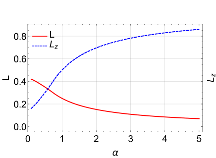
Figure 4: $L$ and $L_{z}$ plotted against $\alpha$ for the hemispheroid.

Plots of the depolarization factors $L$ and $L_{z}$ versus $\alpha$ are displayed in Fig. 4. As $\alpha$ increases, the value of $L$ decreases monotonically whereas the value of $L_{z}$ increases monotonically. For $\alpha<0.569$, $L>L_{z}$; and for $\alpha>0.569$, $L<L_{z}$. In the limit $\alpha\to 0$ we find $L=\left(2+\sqrt{2}\right)/8$ and $L_{z}=\left(2-\sqrt{2}\right)/4$, while in the limit $\alpha\to\infty$ we find $L=0$ and $L_{z}=1$. For $\alpha=1$ the results for the hemisphere are recovered.

4.2 Double-truncated spheroid

Consider the spheroid

$$\frac{x^{2}+y^{2}}{\alpha^{2}}+z^{2}\leq 1,$$ (19)

centered at the coordinate origin with $\alpha>0$. The spheroid is oblate for $\alpha>1$ and prolate for $\alpha<1$. Suppose that the spheroid is trifurcated symmetrically by the planes $z=\pm\kappa$, where $0<\kappa<1$. Then $V_{\delta}$ is the double-truncated spheroid bounded by the planes $z=\pm\kappa$, as shown in Fig. 1(e). The largest inscribed sphere is centered at the origin of the coordinate system.

Equation (5) yields $\underline{\underline{L}}=L\left(\hat{{\bf u}}_{\rm x}\hat{{\bf u}}_{\rm x}+\hat{{\bf u}}_{\rm y}\hat{{\bf u}}_{\rm y}\right)+L_{z}\,\hat{{\bf u}}_{\rm z}\hat{{\bf u}}_{\rm z}$, where

$$L=\frac{1-L_{z}}{2}=\frac{-\nu+\alpha^{2}\tan^{-1}\nu}{2\left(\alpha^{2}-1\right)^{3/2}}$$ (20)

with

$$\nu=\kappa\sqrt{\frac{\alpha^{2}-1}{\alpha^{2}-\kappa^{2}\left(\alpha^{2}-1\right)}};$$ (21)

and again $L_{z}=1-2L$.

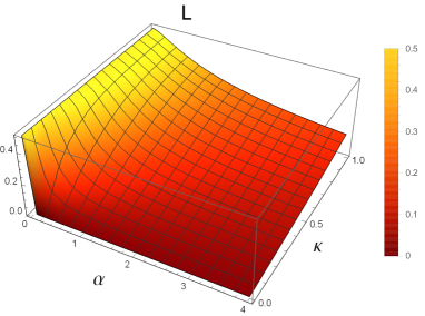
Figure 5: $L$ plotted against $\alpha\in(0,4]$ and $\kappa\in(0,1)$ for the double-truncated spheroid.

In Fig. 5, the depolarization factor $L$ is plotted against $\alpha$ and $\kappa$. As $\alpha$ increases, $L$ decreases monotonically and $L_{z}$ increases monotonically, for all values of $\kappa$. As $\kappa$ increases, $L$ increases monotonically and $L_{z}$ decreases monotonically for all values of $\alpha>0$. In the limit $\kappa\to 0$ we find $L=0$ and $L_{z}=1$, while in the limit $\kappa\to 1$ we find

$$L=\frac{1}{2}\left(\frac{1}{1-\alpha^{2}}+\alpha^{2}\frac{\tan^{-1}\sqrt{\alpha^{2}-1}}{\left(\alpha^{2}-1\right)^{3/2}}\right),$$ (22)

in agreement with the standard results for spheroids [8]. In the limit $\alpha\to 0$, $L=1/2$ and $L_{z}=0$; while $L=0$ and $L_{z}=1$ in the limit $\alpha\to\infty$. And the results for the hemisphere are recovered with $\alpha=1$.

5 Ellipsoidal geometry

In the cases of truncated ellipsoidal geometries, closed-form expressions for $L_{x}$, $L_{y}$, and $L_{z}$ could not be obtained, but numerical methods were used to evaluate these depolarization factors.

5.1 Hemi-ellipsoid

Consider the ellipsoid

$$\frac{x^{2}}{\alpha^{2}}+\frac{y^{2}}{\beta^{2}}+\left(z+\kappa\right)^{2}\leq 1.$$ (23)

with $\alpha>0$, $\beta>0$, and $0\leq\kappa\leq 1/2$. Suppose that the ellipsoid is truncated by the symmetry plane $z=-\kappa$. We chose $V_{\delta}$ as the upper hemi-ellipsoid bounded below by the plane $z=-\kappa$. The largest inscribed sphere is specified by Eq. (9) with radius

$$\kappa=\left\{\begin{array}[]{lcr}1/2,&\mbox{for}&\alpha>1/\sqrt{2},\quad\beta>1/\sqrt{2}\vspace{8pt}\\ \alpha\sqrt{1-\alpha^{2}}&\mbox{for}&\alpha\leq 1/\sqrt{2},\quad\alpha<\beta\vspace{8pt}\\ \beta\sqrt{1-\beta^{2}}&\mbox{for}&\beta\leq 1/\sqrt{2},\quad\beta<\alpha\end{array}\right..$$ (24)

In Fig. 6, plots of the depolarization factors $L_{x}$ and $L_{y}$ versus $\alpha$ and $\beta$ are displayed; the plot of $L_{z}$ may be inferred from $L_{z}=1-L_{x}-L_{y}$. All depolarization factors vary smoothly as $\alpha$ and $\beta$ increase. In particular, $L_{x}$ decreases markedly as $\alpha$ increases but is relatively insensitive to changes in $\beta$; $L_{y}$ decreases markedly as $\beta$ increases but is relatively insensitive to changes in $\alpha$; and $L_{z}$ generally increases as both $\alpha$ and $\beta$ increase.

5.2 Double-truncated ellipsoid

Consider the ellipsoid

$$\frac{x^{2}}{\alpha^{2}}+\frac{y^{2}}{\beta}+z^{2}\leq 1,$$ (25)

centered at the origin of the coordinate system with $\alpha>0$ and $\beta>0$. Suppose that the ellipsoid is trifurcated by the planes $z=\pm\kappa$, where $0<\kappa<1$. Then $V_{\delta}$ is the double-truncated ellipsoid bounded by the planes $z=\pm\kappa$, and the largest inscribed sphere is centered at the origin of the coordinate system.

For $\kappa\in\left\{0.1,0.5,0.9\right\}$, plots of $L_{x}$ and $L_{y}$ versus $\alpha$ and $\beta$ are provided in Fig. 7; the plot of $L_{z}$ may be inferred since $L_{z}=1-L_{x}-L_{y}$. The plots in Fig. 7 for the double-truncated ellipsoid are qualitatively similar to those in Fig. 6 for the hemi-ellipsoid. The effects of varying $\kappa$ are most appreciable at low values of $\alpha$ for $L_{x}$, at low values of $\beta$ for $L_{y}$, and at low values of both $\alpha$ and $\beta$ for $L_{z}$. Generally, the values of the depolarization factors $L_{x}$, $L_{y}$, and $L_{z}$ are substantially more sensitive to variations in $\alpha$ and $\beta$ than they are to variations in $\kappa$.

6 Closing remarks

Depolarization dyadics are central to theoretical studies in scattering and homogenization, but closed-form expressions for these entities have been available only for a few simple shapes. Closed-form expressions for depolarization dyadics have been developed herein for truncated spheres and truncated spheroids, and the formalism has been extended to truncated ellipsoids; the evaluation of depolarization dyadics for this latter case requires numerical integration. These theoretical results will enable studies of scattering from complex-shaped small particles [19] as well as of homogenization of particulate composite materials containing complex-shaped particles [6]. These results are particular valuable in view of the ongoing rapid development of nanocomposite materials for optical applications [20].

Acknowledgments: TGM was supported by EPSRC (grant number EP/V046322/1). AL was supported by the US National Science Foundation (grant number DMS-1619901) as well as the Charles Godfrey Binder Endowment at Penn State.

Declaration of competing interest: The authors declare that they have no known competing financial interests or personal relationships that could have appeared to influence the work reported in this paper.

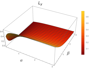
Figure 6: $L_{x}$ and $L_{y}$ plotted against $\alpha\in(0,3]$ and $\beta\in(0,3]$ for the hemi-ellipsoid.

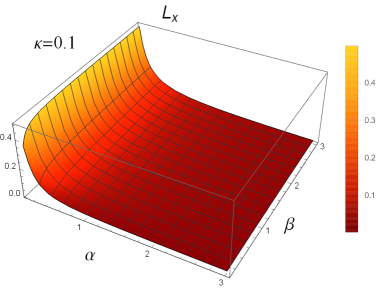
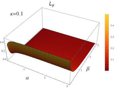
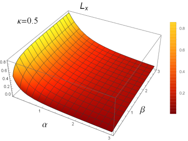
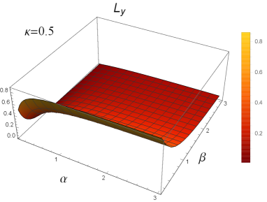
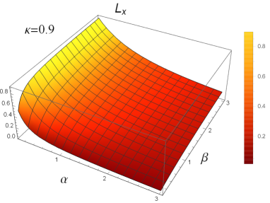
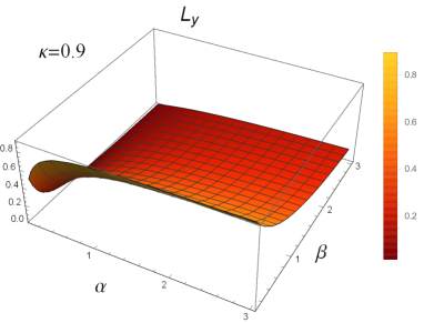
Figure 7: $L_{x}$ and $L_{y}$ plotted against $\alpha\in(0,3]$ and $\beta\in(0,3]$ for the double-truncated ellipsoid with $\kappa\in\left\{0.1,0.5,0.9\right\}$.

References

- [1] H.C. Chen, Theory of Electromagnetic Waves. New York, NY, USA: McGraw–Hill, 1983.
- [2] C.T. Tai, Dyadic Green Functions in Electromagnetic Theory, 2nd Ed. Piscataway, NJ, USA: IEEE Press, 1994.
- [3] M. Faryad and A. Lakhtakia, Infinite-Space Dyadic Green Functions in Electromagnetism. San Rafael, CA, USA: Morgan & Claypool, 2018.
- [4] J. Van Bladel, Singular Electromagnetic Fields and Sources. Oxford, UK: Oxford University Press, 1991 (reissued in association with IEEE Press, New York, NY, USA, 1995).
- [5] T.G. Mackay and A. Lakhtakia, Electromagnetic Anisotropy and Bianisotropy: A Field Guide, 2nd Ed. Singapore: World Scientific, 2019.
- [6] T.G. Mackay and A. Lakhtakia, Modern Analytical Electromagnetic Homogenization with Mathematica, 2nd Ed. Bristol, UK: IOP Publishing, 2020.
- [7] B. Michel, “A Fourier space approach to the pointwise singularity of an anisotropic dielectric medium,” Int. J. Appl. Electromagn. Mech., vol. 8, pp. 219–227, 1997.
- [8] A. Moroz, “Depolarization field of spheroidal particles,” J. Opt. Soc. Am. B, vol. 26, pp. 517–527, 2009.
- [9] J.A. Osborn, “Demagnetizing factors of the general ellipsoid,” Phys. Rev., vol. 67, pp. 351–357, 1945.
- [10] E.C. Stoner, “The demagnetizing factors for ellipsoids,” Phil. Mag., vol. 36, pp. 803–821, 1945.
- [11] B. Michel and W.S. Weiglhofer, “Pointwise singularity of dyadic Green function in a general bianisotropic medium,” Arch. Elektr. Übertrag., vol. 51, pp. 219–223, 1997. Corrections: vol. 52, p. 310, 1998.
- [12] W.S. Weiglhofer, “Electromagnetic depolarization dyadics and elliptic integrals,” J. Phys. A: Math. Gen., vol. 31, pp. 7191–7196, 1998.
- [13] S.W. Lee, J. Boersma, C.L. Law, and G.A. Deschamps, “Singularity in Green’s function and its numerical evaluation,” IEEE Trans. Antennas. Propagat., vol. 28, pp. 311–317, 1980.
- [14] W.S. Weiglhofer and T.G. Mackay, “Needles and pillboxes in anisotropic mediums,” IEEE Trans. Antennas Propagat., vol. 50, pp. 85–86, 2002.
- [15] A. Lakhtakia and N.S. Lakhtakia, “A procedure for evaluating depolarization dyadics of polyhedra,” Optik, vol. 109, pp. 140–142, 1998.
- [16] J.J.H. Wang, “A unified and consistent view on the singularities of the electric dyadic Green’s function in the source region,” IEEE Trans. Antennas Propagat., vol. 30, 463–468, 1982.
- [17] A.D. Yaghjian, “Electric dyadic Green’s function in the source region,” Proc. IEEE, vol. 68, pp. 248–263, 1980.
- [18] J. Avelin, A. N. Arslan, J. Brännback, M. Flykt, C. Icheln, J. Juntunen, K. Kärkkäinen, T. Niemi, O. Nieminen, T. Tares, C. Toma, T. Uusitupa, and A. Sihvola, “Electric fields in the source region: the depolarization dyadic for a cubic cavity,” Elec. Eng., vol. 81, pp. 199–202, 1998.
- [19] C.F. Bohren and D.R. Huffman, Absorption and Scattering of Light by Small Particles. New York: Wiley, 1983,
- [20] M.P. Mengüç and M. Francoeur (Eds.), Light, Plasmonics and Particles. Amsterdam: Elsevier, 2023.