In situ Remnants of Solar Surface Structures from Jensen-Shannon Scalogram

Abstract

The heliosphere is permeated with highly structured solar wind originating from the sun [7]. One of the primary science objectives of Parker Solar Probe (PSP) is to determine the structures and dynamics of the plasma and magnetic fields at the sources of the solar wind [18]. However, establishing the connection between in situ measurements and structures and dynamics in the solar atmosphere is challenging: most of the magnetic footpoint mapping techniques have significant uncertainties in the source localization of a plasma parcel observed in situ [39; 4; 5], and the PSP plasma measurements suffer from a limited field of view [26; 36]. Therefore it lacks a universal tool to self-contextualize the in situ measurements. Here we develop a novel time series visualization method named Jensen-Shannon Scalogram. Utilizing this method, by analyzing the magnetic magnitude data from both PSP and Ulysses [10], we successfully identify in situ remnants of solar atmospheric and magnetic structures spanning more than seven orders of magnitude, from years to seconds, including polar and mid-latitude coronal holes, [35; 5; 14] as well as structures compatible with super-granulation [9], “jetlets” [40; 48] and very small scale flaring activity [13]. Furthermore, computer simulations of Alfvénic turbulence support key features of the observed magnetic magnitude distribution. Building upon these discoveries, the Jensen-Shannon Scalogram therefore not only enables us to reveal the fractal fine structures in the solar wind time series from both PSP and decades-old data archive, but will also serve as a general-purpose data visualization method applicable to all time series.

Main

The solar atmosphere is highly structured both spatially and temporally [7; 27]. Recent studies have successfully established connections between PSP in situ observations and solar atmospheric structures including mid-latitude coronal holes [5; 14], pseudostreamers [28], and supergranulation [8; 17; 9], even though alternative explanations remain [44]. Recent advances in remote sensing provide strong support for the minutes long small-scale jetting activity from magnetic reconnection (“jetlets”) as a major source of the solar wind [40]. In addition, EUV observations from Solar Orbiter [37] unveiled ubiquitous brightening termed “picoflare” [13] with associated jets that last only a few tens of seconds, suggesting the solar wind source might be highly intermittent. However, magnetic footpoint mapping methods [4; 39; 5] use photospheric magnetic field observations over the whole visible disk that are refreshed at best once every six hours and lack, of course, any real temporal reliability for the far side. Therefore, such methods are hardly able to reliably contextualize and explain the boundaries of the highly structured solar wind in situ time series, except perhaps in a statistical sense.

Two of the most interesting yet overlooked features of the time series of the solar wind magnetic field magnitude $B$ are that: 1. Sometimes $B$ displays a surprisingly stable power law dependence on the heliocentric distance $R$; 2. By applying a helio-radial power law fit between $B$ and $R$, i.e. $B\propto R^{-s}$, the fit normalized magnetic magnitude $B^{*}=B(R/R_{0})^{s}$ sometimes displays a near-perfect Gaussian distribution. This is demonstrated in Figure 1 (a-c), where the selected interval is highlighted with a golden bar in panel (a) and the helio-radial power law fit (fit index $s=1.86$) is shown in the inset figure. The histogram of $B$ is shown in blue in panel (b) and the normalized $B^{*}$ is shown in red. To illustrate the close proximity of the probability density function of $B^{*}$ ($PDF_{B^{*}}$) to a Gaussian distribution ($\mathcal{N}$), a Gaussian curve is overplotted in panel (c) (shifted with the mean value $\langle B^{*}\rangle$ and scaled with the standard deviation $\sigma_{B^{*}}$). The Jensen-Shannon Distance (JSD), a statistical distance metric between probability density functions [32], is calculated between $PDF_{B^{*}}$ and $\mathcal{N}$ to be $JSD(PDF_{B^{*}},\mathcal{N})=10^{-1.431}$, indicating considerable closeness (see Benchmark in Methods). In addition, this highly Gaussian $B^{*}$ interval coincides with the radial solar wind speed profile visualized with radial colored lines in panel (a) and Figure 10c (compiled with SPAN-ion from SWEAP suite [26]). From Nov-17 to Nov-20, the spacecraft was immersed in the high speed solar wind. The JSD produced by this process is represented as one pixel (tip of the green pyramid) in the Jensen-Shannon Scalogram (JS Scalogram) shown in panel (d3), and the scalogram for the corresponding helio-radial power law fit index $s$ is displayed in panel (d4).

Identifying Coronal Holes from in situ Timeseries

Each pixel in the JS scalogram is characterized by a timestamp ($t_{mid}$) and window size ($win$). The step size in $win$ (vertical axis) is chosen to be twice the step size in $t_{mid}$ (horizontal axis), and thus the time range covered by one pixel corresponds to the same time range covered by three pixels in the following row, and so on towards the smallest scales. Therefore, if an interval and the nested sub-intervals possess similar characteristics (e.g. relatively small JSD regardless of $t_{mid}$ and $win$ within the interval), a pyramidal structure is expected from the JS scalogram, and the base of the pyramid indicates the start and end time of the interval. One example is highlighted by the green dashed pyramid in panel (d3), where the tip of the pyramid is in fact selected a posteriori as the local minimum in the JS scalogram ($PDF_{B^{*}}$ being closest to Gaussian). Ample information can be inferred from the JS scalogram: 1. A semi-crossing of the heliospheric current sheet (HCS) at noon of Nov-22 is visualized as an inverted black pyramid; 2. It is well-known that the solar wind sourced from a single mid-latitude coronal hole from Nov-17 to the end of Nov-20, and from another coronal hole for the whole day of Nov-21 [39; 5; 9]. The coronal holes are naturally visualized here as two white pyramids (green and red dashed lines) separated by a dark region around the mid-night of Nov-20; 3. The helio-radial power law fit index $s$ is unexpectedly stable and systematically deviates from $R^{-2}$ ($s\simeq 1.87\pm 0.02$).

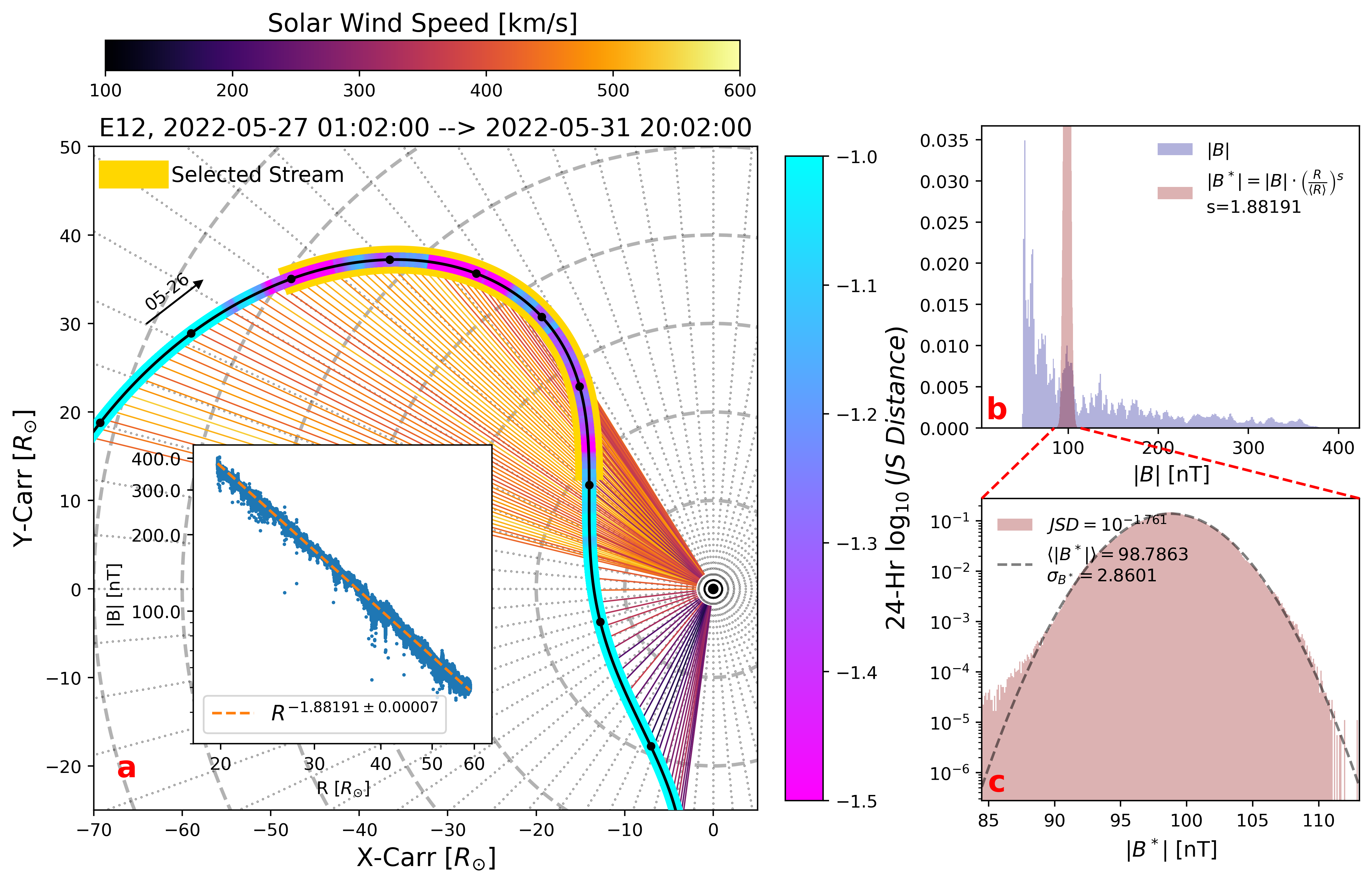
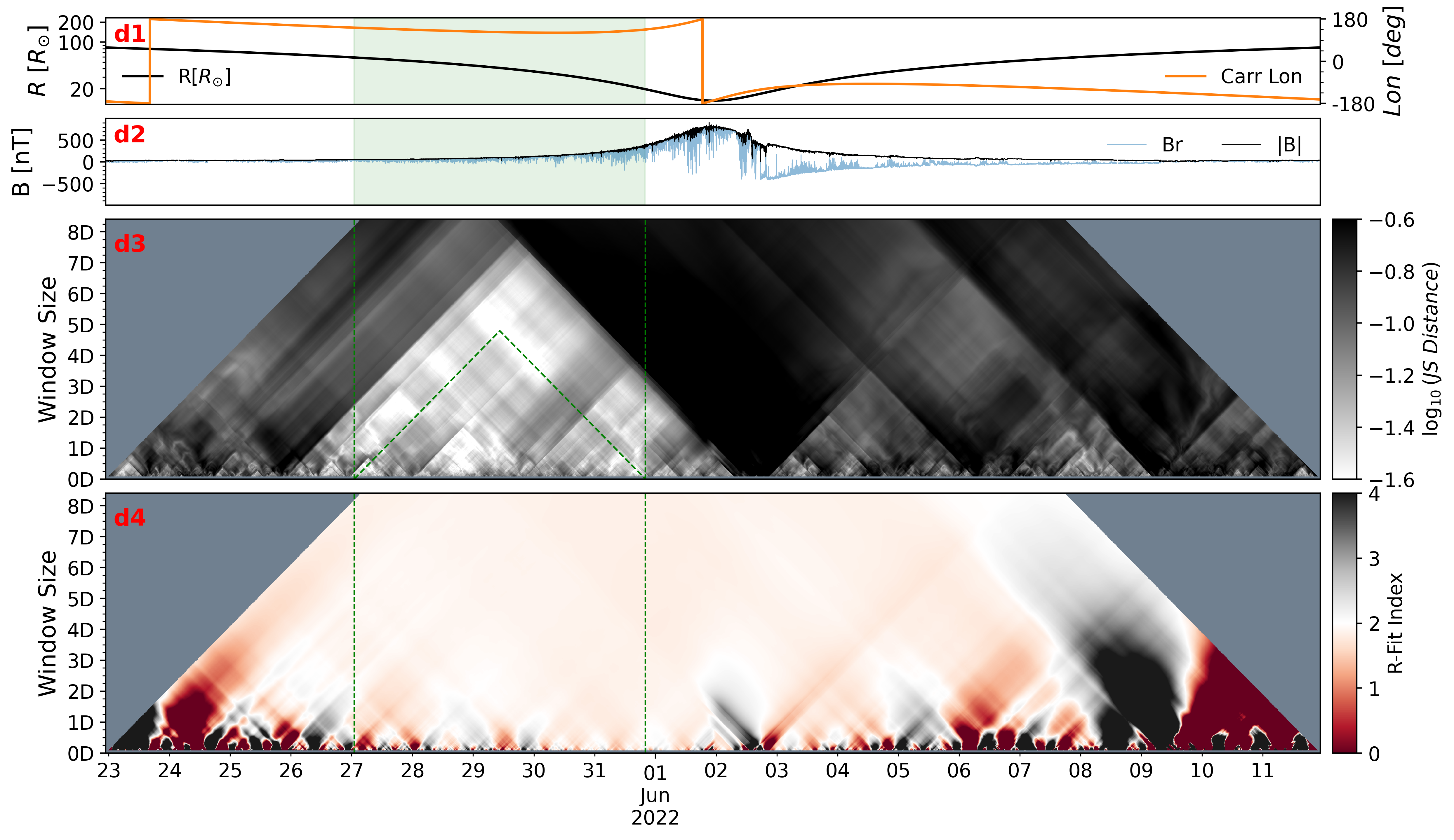
Figure 12: Selected interval from E12.

The clear correspondence between the white pyramid and coronal hole encourages us to predict intervals of solar wind originating from coronal holes with JS scalograms compiled from PSP data. Unfortunately, among the first 14 encounters (Nov-2018 to Dec-2022), we only identified one more (for a total of 2) long intervals ($>$ 3 days) characterized by high Gaussianity in $B^{*}$. A panoramic view of these two long intervals is shown in Figure 10. The newly found interval from the inbound of E12, shown in Figure 12 and Figure 10 (d), is characterized by a 5-day long highly Gaussian $B^{*}$ time series. For illustration purpose, the green pyramid in Figure 12 (d3) is selected as the deepest local minimum in JS scalogram for $win>$ 3 days. The histogram of $B^{*}$ is remarkably concentrated (panel (b)) and aligns with Gaussian almost perfectly within 4 standard deviation (panel (c)). Similar to Figure 1 (c), the non-Gaussian part of $PDF_{B^{*}}$ has a systematic bias towards magnetic holes (weaker magnetic magnitudes), and the helio-radial power law fit index scalogram also shows a systematic deviation from $s=2$, similarly $s\simeq 1.87\pm 0.02$. To validate this prediction, independent results from Potential Field Source Surface (PFSS) model shown in Figure 8 (see [39] for more details) indicate that the selected interval is magnetically connected to a mid-latitude coronal hole.

Figure 1: Selected interval from November 2021, encounter 10 of Parker Solar Probe. Panel (a): This panel presents the spacecraft trajectory in the Carrington corotating frame from the afternoon of November 16, 2021, to the afternoon of November 22, 2021. Each day’s start is indicated with black circles. The ballistic solar wind streamlines are plotted at a 2-hour cadence and colored according to the 10-minute averaged solar wind speed profile from SPAN-ion moment. The selected interval is emphasized with a golden bar, and the 24-Hour window Jensen-Shannon Distance (JSD) of normalized magnetic magnitude $B^{*}$ is represented by the colored band. An inset displays the helio-radial power law dependence of $B$. Panel (b): The histogram of $B$ and $B^{*}$ from the selected interval. Panel (c): The histogram of $B^{*}$ and $JSD(PDF_{B^{*}})$. Panel (d1): Spacecraft heliocentric distance (black) and Carrington longitude (orange). Panel (d2): Magnetic field radial component $B_{r}$ and magnitude $B$. Panel (d3): Jensen-Shannon Distance Scalogram. The selected interval is highlighted with the green pyramid. Panel (d4): Helio-radial power law fit index scalogram of $B$.

Switchback Patches, Jetlets and Picoflares

To substantiate the potential of JS scalogram, we demonstrate here several applications that visualize the fractal spatial-temporal structures in the solar wind (Due to the rapid movement of PSP around perihelia, the structures in the in situ time series can be categorized into two kinds. Spatial: transverse longitudinal structures traversed by PSP; Temporal: radial structures advected by the solar wind and/or propagation of Alfvén waves), from the largest scales: Ulysses, years-long polar coronal hole [35], towards the smallest scales: hour-long switchback patches [8; 17; 44; 9]; minute-long structures compatible with “jetlets” [40]; and second-long structures consistent with “picoflare” [13].

Figure 2: Jensen-Shannon Scalogram from Ulysses first orbit from 1993 to 1998. Panel (a): Ulysses heliocentric distance $R$ (black line) and heliographic latitude colored with local 48-hour averaged solar wind speed. Panel (b): Jensen-Shannon Scalogram compiled from magnetic magnitude $B$ (lower half) and helio-radial power law normalized magnitude $B^{*}$ (upper half). Panel (c): $R_{max}/R_{min}$ of each interval (pixel), the cut-off value is chosen to be $R_{max}/R_{min}=1.5$, beyond which $B$ is normalized into $B^{*}$ using helio-radial power law fit.

Figure 2 shows the JS scalogram of the first Ulysses orbit, and the colorbar in panel (b) is enhanced compared to Figure 1 (d3) for illustration purposes. The solar latitude and wind speed profile in panel (a) indicate that the spacecraft was in southern and northern polar coronal holes in the whole year of 1994, and from 1995 to 1997 (see also [35]). The two large white pyramids in the JS scalogram clearly correspond to the two polar coronal holes. Notably, the boundary observed in panel (b) results from an artificial cut-off in the helio-radial power law fit, as shown in panel (c). For more details on the cut-off boundary, refer to the caption of Figure 2. However, the JSD are much larger in the polar coronal holes compared to the mid-latitude coronal holes observed by PSP at much smaller heliocentric distance, and the histograms of magnetic magnitude show much more significant fat tail towards the magnetic holes side (not shown here). This indicates that the Gaussianity of magnetic magnitudes decreases with increasing heliocentric distance and magnetic holes are much more preferred than spikes in the solar wind.

Figure 3: Jensen-Shannon Scalogram of Parker Solar Probe E10 inbound mid-latitude coronal hole. Panel (a): From top to bottom: Carrington longitude plotted with 1 degree cadence colored with spacecraft angular velocity in the corotating frame (blue: prograde, red: retrograde); JS scalogram with 1-minute resolution; Normalized magnetic magnitude $B^{*}$ and radial component $B_{r}^{*}$; Radial solar wind speed $V_{r}$; Panel (b): Expanded view of panel (a) with 10-second resolution.

Figure 3 shows the hour-long switchback patches from a single mid-latitude coronal hole in PSP E10, which have been recently argued to be the remnants of the solar supergranulation [8; 17; 9]. The Carrington longitude of the spacecraft is plotted every one degree on the top bars of both panels (a) and (b), and the color indicates spacecraft angular velocity in the corotating frame (blue: prograde, red: retrograde). The magnetic magnitude is normalized with a universal helio-radial power law fit index ($s=1.87$) and the JS scalogram is compiled with the full-resolution fluxgate magnetic data ($\sim$ 292 Hz, see [6; 12]). The red dashed pyramids in panel (a) and (b) are drawn to highlight the $B^{*}$ intervals with high level of Gaussianity. The selected intervals in panel (a) show that the JS scalogram effectively captures the switchback patches. When these are compared with the Carrington longitude, it becomes evident that some of the structures align with the size of supergranulation, as discussed in [9]. However, other structures, which are smaller in angular size and likely temporal in nature, could be more accurately attributed to the ’breathing’ phenomenon of the solar wind, as explained in [11; 44]. After the “fast radial scan” phase on Nov-18, the spacecraft began to rapidly retrograde on Nov-19 and Nov-20 (see Figure 1 (a) for the spacecraft trajectory in the corotating frame). For better comparison, an expanded view is shown in panel (b). The second and third pyramids also show decent capability of capturing the switchback patches, whereas the first pyramid seems to capture a boundary between the patches. Starting from 7:00 on Nov-20, the remaining patches consistently exhibit a high level of Gaussianity across all scales and locations, resulting in indistinct boundaries between them.

Figure 4: Hierarchic multi-scale Jensen-Shannon Scalogram illustration of mid-latitude coronal from PSP encounter 12 inbound. For all subplots, the Carrington longitude of the spacecraft is shown in the top panel. For subplots (a) to (c), the bars are plotted every 1 degree, with colors indicating the heliocentric angular velocity in the solar corotating frame (blue: progradation, red: retrogradation). For subplots d and e, the crosses are plotted every 0.1 degree. The corresponding magnetic field magnitude $B$ and radial component $B_{r}$ are shown in the second panel of each subplot; and except for subplot (a), the magnetic field is normalized with helio-radial power law fit. The radial solar wind speed $V_{r}$ is also shown in subplot (b) to (e).

Figure 4 presents a hierarchic JS scalogram of the mid-latitude coronal hole from E12 of PSP. In panels (d) and (e), focusing on the smallest scales resolvable by the Jensen-Shannon distance (approximately 1 minute, corresponding to around 20,000 data points for the shortest interval), we observe a surprising number of structures with distinct boundaries. For details on how the number of data points influences this analysis, see the Methods section. In fact, these structures, typically lasting 1-10 minutes, are omnipresent in the Alfvénic solar wind observed in all PSP encounters. Notably, they are not limited to winds with a clear coronal hole origin, such as those in the outbound paths of E12 (for more details, see the video in the supplementary materials). These structures are typically separated (interrupted) by radial jets (or switchbacks), with these separations frequently accompanied by kinetic-scale ($\lesssim$ 5 seconds) fluctuations that are bursty and short-lived in all three components. Once smoothed, these fluctuations resemble magnetic holes. For further illustration, refer to the skewness scalogram video in the supplementary materials. Unlike the spatial structures shown in panels (a), (b), and (c) (as well as in Figure 1 and Figure 2), the longitude change of the spacecraft for each structure in panel (d) and (e) is less than 0.1 degree, as indicated by the crosses plotted every 0.1 Carrington longitude in the top bar. Therefore, these structures are likely temporal, advected by the solar wind. All of these features are highly compatible with the “jetlets” observed in equatorial coronal holes [40], and therefore could potentially be the “building blocks” of the solar wind. In fact, even finer structures can be found with the normalized standard deviation ($\sigma_{B^{*}}/\langle B^{*}\rangle$) scalogram and skewness scalogram shown in Figure 11. For example, the small white pyramid around 8:36 in Figure 4e has two 30-seconds long substructures nested beneath in Figure 11. These seconds-long structures are intervals with smaller standard deviation compared to the surroundings, and their interruptions are temporally compatible with the “picoflare” [13].

Origin of Gaussian B: Turbulence Relaxation and Magnetic Pressure Balance

These observations indicate that the Alfvénic solar wind is permeated with highly Gaussian magnetic magnitude intervals that are often interrupted by radial jets (switchbacks) every 1-10 minutes. In addition, the magnetic fluctuations inside the intervals often resemble the outward propagating small amplitude linear Alfvén waves. Therefore, it is reasonable to model the system as small amplitude Alfvénic MHD turbulence. Figure 9 shows the temporal evolution of the $JSD(PDF_{B},\mathcal{N})$ of a 3D MHD small amplitude Alfvénic turbulence simulation [42]. The simulation is run with $512^{3}$ periodic box, and is initialized with unidirectional small amplitude linearly polarized Alfvén waves with isotropic wave vector spectrum (see Methods section for more details). At $t=0.00\ t_{A}$ (Alfvén crossing time $t_{A}=L/v_{A}$, where $L$ is the simulation box size), $PDF_{B}$ deviates significantly from a Gaussian distribution due to the small amplitude shear Alfvén wave initialization (fluctuations in $B$ are positive definite). The corresponding JSD is highlighted as the first red dot in the lower panel and is much larger than 0. Surprisingly, within one Alfvén crossing time at $t=0.40\ t_{A}$, the distribution of $B$ rapidly relaxes to a near-perfect Gaussian, and the JSD rapidly drops towards the ground truth value (see Benchmark in Methods). As the simulation evolves, the JSD remains considerably small and thus the distribution of $B$ remains very close to Gaussian. The simulation indicates that Gaussian is the natural relaxation state for magnetic magnitude in small amplitude Alfvénic turbulence, consistent with the ubiquitous 1-10 minutes Gaussian intervals found in the solar wind.

Nevertheless, the simulation suggests that information is fully exchanged within the system, as it propagates at Alfvén speed throughout the simulation box. This allows $B$ to relax to a Gaussian distribution, which occurs within about 0.5 $t_{A}$, the time it takes for Alfvén waves to carry information from the center of the simulation box to its edges. It is not reasonable to assume that the information is fully exchanged for the hours, days or even months long structures shown in Figures 1, 2 and 3, due to the super-Alfvénic nature of the solar wind close to the sun. Beyond the Alfvén surface [28], the information can only propagate radially outwards in the solar wind. Moreover, the structures that last an hour or longer are likely spread spatially and longitudinally. However, Alfvén waves, along with the information they carry, are guided by the background magnetic field, which predominantly points radially outwards around PSP perihelia. Therefore, an alternative explanation is needed for the hour-long (and longer) Gaussian structures. The simplest explanation for the Gaussian $B$ structures originating from coronal holes (mid-latitude coronal holes from E10 and E12, and polar coronal holes from Ulysses) is the pressure balance between the open coronal field lines. Close to the sun, the solar wind originating from the coronal holes is mostly magnetic dominant (plasma $\beta=2\mu_{0}P/B^{2}\ll 1$, see e.g. [28]). Therefore, to maintain pressure balance, the open field lines from the same coronal hole tend to evolve to a state in which the magnetic pressure $P_{B}=B^{2}/2\mu_{0}$ is mostly uniform for a given cross section of the magnetic flux tube. In Figure 1, the helio-radial power law normalization of $B$ essentially maps the magnetic field line density, which is effectively the magnetic flux density due to the spherical polarization of the Alfvén waves, from various radial distances and transverse locations to a single cross-section of the flux tube (for more details, see the Methods section and [33; 34]). As a support of this idea, from the PSP observations of E10 and E12 (Figure 1 and Figure 12), the helio-radial power law normalization of $B$ effectively collapses the histogram of $B$ into a delta-function-like histogram of $B^{*}$. This is indicative of identical field line density within a single coronal hole due to the magnetic pressure balance. The detailed distribution of $B^{*}$ is hence the feature of the noise in magnetic magnitude within the coronal hole, which can be considered as a stopped one-dimensional random walk (additive noise sourced from the base of the corona). Therefore, the Gaussian distribution of $B^{*}$ can be easily explained as the result of the random walk according to central limit theorem. Nevertheless, difficulties remain for the origin of the hour-long structures. They may be the manifestation of the denser field line density originating from a single supergranule, but the more detailed discussion lies beyond the scope of this study.

Finally, the existence of a stable power law dependence of $B$ with regard to heliocentric distance $R$ itself already sheds light on the physics of the solar wind originating from coronal holes. As solar activities ramp up for solar cycle 25, 4 out of the 5 recent encounters (E10, E11, E12, E14) of PSP show systematic preference for a single helio-radial power law index, which confidently deviates from $R^{-2}$. However, the $R^{-2}$ power law, expected only from the dominant radial component $B_{r}$ as a result of the Parker Spiral (conservation of magnetic flux in spherical expansion), is not strictly applicable to $B$, especially for PSP, due to the ubiquitous switchbacks. Due to the relation between $B$ and the local magnetic flux density, this is indicative of a stable expansion rate for the magnetic flux tube in the magnetic dominant wind ($\beta\ll 1$) close to the sun. Such an expansion rate is crucial for the estimation of the WKB evolution of the fluctuation quantities like the magnetic and velocity field [21; 20; 50; 23]. It should be noted that the fit indices of $B$ coincide with the helio-radial dependence of the electron density compiled from Quasi Thermal Noise [29; 36], indicating that the deviation from $R^{-2}$ could be the evidence of active acceleration of the solar wind.

Compiled from the almost featureless magnetic magnitude time series from the solar wind, the Jensen-Shannon scalograms unveiled a striking number of fractal magnetic structures spanning across over seven orders of magnitude in time. These structures include spatial structures like polar coronal holes [35], mid-latitude coronal holes [5], and switchback patches [9]. They also include temporal structures compatible with “jetlets” [40] and “picoflare” [13], which are often interrupted by the radial jets (switchbacks). In addition, three-dimensional MHD simulations have shown that Gaussian is the natural relaxation state for small amplitude unidirectional Alfvénic turbulence. The minute-long structures are hence likely to be the natural products of Alfvénic MHD turbulence. Thus, it is now clear that the Alfvénic solar wind is permeated with these intermittent Gaussian $B$ structures, which are self-similarly organized from seconds to years, and are likely the remnants of the magnetic structures on the solar surface [47; 2; 3; 9; 40; 13]. This paper reveals just a fraction of the rich structures uncovered by the JS scalogram from the solar wind time series. The JS scalogram proves to be a versatile tool, essential not only for deciphering the structure and dynamics of plasma and magnetic fields—key objectives of the PSP mission [18]—but also for revitalizing decades-old solar wind data from missions like Helios, Ulysses, and WIND. These efforts unveil new physics previously hidden within these data sets. Additionally, the JS scalogram’s applicability extends beyond solar wind analysis, serving as an effective general-purpose method for visualizing a wide range of time series data.

Methods

Jensen-Shannon Distance, Jensen-Shannon Scalogram and Benchmark

Figure 5: Benchmark of all three free parameters: number of standard deviation $\sigma$, number of bins, and number of points. Panel (a): the Jensen-Shannon distance between a given probability distribution function and the standard Gaussian distribution $\mathcal{N}(0,1)$; Panel (b): the “Ground Truth” values, i.e. the JS distance of the histogram with $N_{b}$ number of bins estimated from $N_{p}$ number of points from $\mathcal{N}(0,1)$; Panel (c): the same x and y bins as panel (b), with values of $JSD(PDF_{Logistic}\parallel\mathcal{N}(0,1))$.

The Jensen-Shannon Distance is the square root of Jensen-Shannon Divergence [32] which is the symmetrized and smoothed version of Kullback–Leibler Divergence [30]. Due to its symmetry and smoothness, Jensen-Shannon Distance is an ideal metric for the similarity between the observed magnetic magnitude distribution and the Gaussian distribution. For two discrete probability distribution functions $P$ and $Q$ defined in the same space $\mathcal{X}$, the Jensen-Shannon Divergence is calculated as following:

$$\mathrm{JSD}(P\|Q)=\frac{1}{2}D_{\mathrm{KL}}(P\|M)+\frac{1}{2}D_{\mathrm{KL}}(Q\|M)$$ (1)

where $M=(P+Q)/2$ is the mixture distribution of $P$ and $Q$, and $D_{\mathrm{KL}}(P\|Q)$ is the Kullback–Leibler Divergence:

$$D_{\mathrm{KL}}(P\|Q)=\sum_{x\in\mathcal{X}}P(x)\log\left(\frac{P(x)}{Q(x)}\right)$$ (2)

In this study, we use scipy.spatial.distance.jensenshannon [51] to calculate the Jensen-Shannon Distance. This program uses natural base logarithm in Kullback–Leibler Divergence, and therefore the final Jensen-Shannon distance is bounded by $[0,\sqrt{ln(2)}]$.

The Jensen-Shannon scalogram (JS scalogram) is a map where the vertical axis is window size ($win$) and the horizontal axis is the central time of each interval ($t_{mid}$), together forming a scalogram of Jensen-Shannon distance between the normalized probability density function of a given interval $PDF(t_{mid},win)$ and the standard Gaussian distribution $\mathcal{N}(0,1)$, i.e. $JSD(PDF(t_{mid},win),\mathcal{N}(0,1))$, or simply $JSD(PDF,\mathcal{N})$. To calculate $PDF(t_{mid},win)$ from the ensemble of samples from a given interval, there are three controlling parameters: sample size $N_{p}$, number of bins $N_{b}$, and number of standard deviation considered $\sigma$. In addition, for benchmark purposes, it is necessary to calculate the JSD between some well-known symmetric distributions and standard Gaussian distribution. The summary of the influence of the controlling parameters and the comparison with well-known distributions are shown in Figure 5.

The JSD between Laplace and Logistic distributions and Gaussian distribution as a function of standard deviation range considered is shown in panel (a). The JSD value stablizes approximately at 5 $\sigma$, and therefore for all JS scalograms shown in this paper, the $PDF$ are all compiled for $\pm 5\sigma$. To see how $N_{p}$ and $N_{b}$ control the JSD value, samples are repeated drawn from a true Logistic distribution to calculate $JSD(Logistic,\mathcal{N}|N_{p},N_{b})$. In panel (c), we see a much stablized region for large enough $N_{p}$ and not-too-large $N_{b}$ (The stable region is orange-ish because theoretical value at 5 $\sigma$ is slightly smaller than the true value shown in panel (a) as dark red horizontal dashed line). Two purple dashed regions are highlighted in panel (c), where the right one indicates the parameter space used for low resolution JS scalogram shown in Figure 1 and 12, and the left one corresponds to the high resolution version shown in Figure 4 (c-e).

In addition, $N_{p}$ and $N_{b}$ also influence the ground truth value, i.e. the Jensen-Shannon distance between an ensemble statistically drawn from Gaussian generator and the real Gaussian PDF, which is not available in closed form [38]. To obtain the ground truth value, the PDF is a histogram of equally spaced $N_{b}$ bins located within $\pm$ 5 $\sigma$ compiled from $N_{p}$ independent samples drawn from a standard Gaussian source numpy.random.randn [19], and then the JSD is the averaged distance between the statistically calculated PDF($N_{p},N_{b}$) (repeated 30 times for each $N_{p}$ and $N_{b}$) and the true Gaussian PDF. The standard deviation is found to be small for a given tuple of $N_{p}$ and $N_{b}$. The resulting $N_{p}$-$N_{b}$ map is shown in panel (b), and the two parameter space considered are also shown as purple dashed regions. Even for the poorest case ($N_{p}\sim 20000$), the ground truth value is still sufficiently away from JSD($Logistic,\mathcal{N}$).

Spherical Polarization of Alfvén Waves

Figure 6: Spherical Polarization of Alfvén waves

Although spherical (arc) polarization of Alfvén waves is well-known [15; 41; 49; 46; 52; 16; 25; 22; 45], for completeness, here we provide a simple model for the spherically polarized Alfvén waves in the magnetically dominated plasma (plasma $\beta=2\mu_{0}P/B^{2}\lesssim 0.1$, typical for Alfvénic solar wind measured by PSP around perihelion [28]) to contextualize the switchbacks and its relation to conservation of magnetic flux. Similar to [33], this model consider the background magnetic field $\vec{B}_{0}$ to be the same as the constant magnetic magnitude $|B|$, but is different from [22] where $\vec{B}_{0}$ is calculated as the spatial average $\langle\vec{B}\rangle$.

For the fluctuation-free magnetic flux tube originated from a coronal hole, the magnetic field is pointing mostly radially higher in the corona and in the solar wind close to the sun. The spherically polarized Alfvén waves can therefore be considered as perturbations to this otherwise quiet system. To maintain the constant $B$ state observed in the solar wind, the additive magnetic perturbation has to “switchback” on top of the radial background field. This scenario is depicted in Figure 6. The constant magnetic magnitude $B$ is shown as the radius of the circle and the static radial field from coronal hole is $\boldsymbol{B}_{0}$. To maintain the constant $B$ state, the perturbation to the system $\boldsymbol{B}_{1}$ is restricted to the semi-circle, and the resultant magnetic vector $\boldsymbol{B}=\boldsymbol{B}_{0}+\boldsymbol{B}_{1}$ can thus fluctuate on a constant sphere of $B$. Following this setup, the magnetically dominant ($p\ll B^{2}/2\mu_{0}$) incompressible MHD equations can be rewritten as follows ($\rho=const$, $p=const$, $B^{2}=const$, $\vec{B}=\vec{B}_{0}+\vec{B}_{1}$):

$$\frac{\partial\vec{u}}{\partial t}=\vec{b}\cdot\nabla\vec{b}-\vec{u}\cdot\nabla\vec{u}$$ (3)

$$\frac{\partial\vec{b}}{\partial t}=\vec{b}\cdot\nabla\vec{u}-\vec{u}\cdot\nabla\vec{b}$$ (4)

where $\vec{b}=\vec{B}/\sqrt{\mu_{0}\rho}=\vec{B}_{0}/\sqrt{\mu_{0}\rho}+\vec{B}_{1}/\sqrt{\mu_{0}\rho}=\vec{b}_{0}+\vec{b}_{1}$. Assuming the frame is co-moving with the bulk flow and the perturbations are Alfvénic, i.e. $\vec{u}=\vec{u}_{1}$ and $\vec{u}_{1}=\pm\vec{b}_{1}$, the equations can be further reduced into a wave equation:

$$\frac{\partial^{2}\vec{b}_{1}}{\partial t^{2}}=(\vec{v}_{a}\cdot\nabla)^{2}\vec{b}_{1}$$ (5)

where $\vec{v}_{a}=\vec{b}_{0}=\vec{B}_{0}/\sqrt{\mu_{0}\rho}$. This equation is identical to the circularly polarized shear Alfvén wave equation, except that $\vec{B}_{1}$ can be large but restricted to a semi-circle and the Alfvén phase velocity $\vec{v}_{a}$ is precisely defined (not defined with time-averaged field).

This model leads to some important implications: 1. The spherically polarized Alfvén wave is an exact solution and is mathematically identical to the small amplitude shear Alfvén mode; 2. If radial jet is present in the system, i.e. $\vec{u}_{1r}\parallel\vec{B}_{0}$, in accordance with the observed “switchbacks”, the spherically polarized Alfv́en waves can only be outward-propagating. This is because to maintain the constant $B$ state, the only possible polarization is $\vec{u}_{1}=-\vec{B}_{1}/\sqrt{\mu_{0}\rho}$; 3. There exists a well-defined background field $\vec{B}_{0}$ for the constant $B$ state, and hence the constant magnetic magnitude $B$ can be regarded as a good proxy for the local $\vec{B}_{0}$, i.e. the local magnetic flux density.

In fact, the reversal of the magnetic field line (switchback) does not increase the number of field lines (thus field line density) and the Alfvén wave, being a solenoidal mode, is not possible to change the local magnetic flux density. This establishes a connection between the magnetic magnitude (magnetic field line density) and the local magnetic flux density within the magnetically dominated coronal holes close to the sun. The helio-radial normalization of $B$ in the main text can therefore be regarded as mapping the magnetic flux density measured at different radial distances and longitudinal locations back to a cross section of the magnetic flux tube originated from the coronal hole.

PSP and Ulysses Data Analysis

The Jensen-Shannon scalograms in this paper are compiled from magnetic magnitude time series of PSP and Ulysses. The fluxgate magnotometer of PSP [6; 12] offers two versions of level-2 data in RTN coordinates: mag_rtn_4_per_cyc and mag_rtn. The JS scalograms for intervals longer than one day are compiled with the low resolution (4 samples per 0.874 second) data product and the rest are compiled with the high resolution (256 samples per 0.874 second) mag_rtn. All magnetic magnitude data points for each interval are treated as independent samples drawn from a stochastic source and therefore the invalid (NaN) values are discarded and no interpolation is applied. The Ulysses magnetic field data is treated the same way.

Three-Dimensional MHD Alfvénic Turbulence Simulation

The simulation is conducted using a 3D Fourier-transform based pseudo-spectral MHD code [43]. MHD equation set in conservation form is evolved with a third-order Runge-Kutta method. A detailed description of the simulation set-up and normalization units can be found in [42]. Here we briefly summarize the key parameters.

The domain of the simulation is a rectangular box with the length of each side being $L=5$. The number of grid points along each dimension is $512$. To ensure numerical stability, explicit resistivity and viscosity $\eta=\nu=2\times 10^{-5}$ are adopted besides a de-aliasing.

For the initial configuration, uniform density, magnetic field and pressure are added: $\rho_{0}=B=1$, $P_{0}=0.1006$. The magnetic field has a small angle ($8.1^{\circ}$) with respect to $x$-axis, and it is inside $x-y$ plane. On top of the background fields, we add correlated velocity and magnetic field fluctuations, i.e. the fluctuations are Alfvénic, with 3D isotropic power spectra. The reduced 1D spectra roughly follow $|k|^{-1.3}$. The strength of the fluctuations is $b_{rms}/B\approx 0.14$ where $b_{rms}$ is the root-mean-square of the magnetic field fluctuation.

Fluxgate Magnotometer Noise and Zeros-Drift

Figure 7: Jensen-Shannon scalogram of magnetic magnitude from the fluxgate magnotometer noise. From top to bottom: magnetic magnitude $B$ timeseries; JS scalogram of $B$; standard deviation scalogram of $B$.

There are several sources of error in the PSP fluxgate magnetometer measurements [6], including the instrumental noise as well as uncertainty in the zero offsets which drift in time [12]. The instrumental noise of each vector component is approximated as Gaussian white noise with a standard deviation $\sigma\simeq 0.05nT$, and together produce a noise with a standard deviation of $\sigma_{noise}\sim 0.1nT$ for the magnetic magnitude. $\sigma_{noise}$ is usually much smaller than the standard deviation of the in situ measured $\sigma_{B}$ for all scales that we are interested in. Nevertheless, the JS scalogram of a ground measured one-hour magnetic field time series for calibration is shown in Figure 7. The distribution of the noise signal is universally Gaussian regardless of scales and location, and the standard deviations are unanimously small. Therefore, most of the Gaussian structures we show in the paper are real signals rather than instrument noise.

The error from drifting spacecraft offsets is a significantly larger contribution to the error as the approximated zero-offsets drift over time and are calibrated each day [12]. The drift of the spacecraft offsets, which is thought to occur due to slowly varying currents on the spacecraft is not well constrained and varies over time. This error is not Gaussian in nature, but should introduce small offsets in the measured field from the real background magnetic field. Spacecraft rolls are used to determine zero-offsets in both the inbound and outbound phases of each orbit, and are updated daily through optimizing the measurements to ensuring that spherically polarized magnetic field intervals maintain a constant magnitude. Typical offset values drift about $0.5nT$/day. Due to the continuous drift and non-Gaussian nature, the sub-day ($\lesssim 5Hr$) structures are not strongly affected by the zeros-drift. And the days-long structures are also not affected because of the instrument calibration of the zeros-offset.

Supplementary Materials

Supplementary Videos

This manuscript contains two supplementary videos: js_scalogram_E12.mp4 and skewness_scalogram_E12.mp4.

js_scalogram_E12.mp4 shows the Jensen-Shannon scalogram and normalized standard deviation scalogram of magnetic magnitude with window sized from 30 second to 15 minutes for the whole Parker Solar Probe E12. This video aims to show the self-similar magnetic structures revealed by JS scalogram and the corresponding sub-structures from the normalized standard deviation scalogram. For the first one minute, the JS scalogram looks different because of the low sampling rate of the fluxgate magnetometer.

skewness_scalogram_E12.mp4 shows the Skewness scalogram and normalized standard deviation scalogram of magnetic magnitude with window sized from 1 second to 5 minutes for the whole Parker Solar Probe E12. This video aims to show the systematic tendency for magnetic holes in the magnetic magnitude distributions.

Supplementary Figures

Figure 8: Magnetic field connectivity with the solar sources during inbound of PSP encounter 12. The thick black lines are the model neutral lines. Black contours indicate magnetic field pressure at 1.05 $R_{s}$. The ballistic projection of the PSP trajectory (blue diamonds) on the source surface (blue crosses) and down to the solar wind source regions (blue circles) is calculated for source surfaces $R_{ss}/R_{s}$ = 2.5 (see [39] for details) and measured in situ solar wind speed ± 80 km s−1. Open magnetic field regions are shown in blue (negative) and green (positive).

Figure 9: Relaxation of magnetic magnitude $B$ in Alfvénic MHD turbulence simulation. Upper panels: (Left) Probability distribution of $B$ ($PDF_{B}$) at $t=0.00\ t_{A}$, where $t_{A}=L/v_{A}$ is the Alfvén time and $L$ is the size of simulation box, $v_{A}$ is the Alfvén speed; (Right) $PDF_{B}$ at $t=0.40\ t_{A}$. Lower panel: Time evolution of the Jensen-Shannon Distance between $PDF_{B}$ and Gaussian Distribution (blue line), and the normalized standard deviation of $B$ (dash dotted line). The time axis is normalized with the Alfvén time $t_{A}$. The simulation time step of the upper left and right panels are highlighted with two red circles in the lower panel.

Figure 10: Panoramic plot of the data considered in this study. Panel (a): This panel shows the heliocentric distance of the spacecraft from encounter 1 to 14. The data analyzed in this study is from $\pm$ 10 days around the perihelia, which are highlighted with black lines and pink shaded areas. The two normally distributed long intervals under investigation are represented by the two green segments. Panel (b): This panel provides a detailed illustration of E10 to E12, with the spacecraft’s angular velocity in the Carrington corotation frame displayed on the twin axis. The corotating periods ($\omega<10\ [deg/Day]$) are marked with golden shaded areas, and the selected intervals are highlighted in green on top of the angular velocity profile. Panel (c) and (d): These panels provide a synopsis plot of E10 and E12 spacecraft trajectories from $\pm$ 8 days around the perihelion in the Carrington corotating frame. The starts of each day are indicated by black dots, and the two arrows show the spacecraft’s entering directions, with the corresponding dates highlighted by red circles. The solar wind streamlines are colored according to the 10-minute averaged solar wind speed and are plotted every 2 hours. The two selected intervals are also highlighted in green.

Figure 11: Skewness and normalized standard deviation scalogram. From top to bottom: spacecraft carrington longitude plotted with 0.1 degree cadence; magnetic magnitude ($B$, black) and radial component ($B_{r}$, blue); radial solar wind speed ($V_{r}$); skewness scalogram of $B$; normalized standard deviation scalogram of $B$

References

- Angelopoulos et al. [2019] Angelopoulos, V., Cruce, P., Drozdov, A., et al. 2019, Space Science Reviews, 215, 9, doi: 10.1007/s11214-018-0576-4
- Aschwanden [2011] Aschwanden, M. 2011, Self-Organized Criticality in Astrophysics: The Statistics of Nonlinear Processes in the Universe (Berlin, Heidelberg: Springer Berlin Heidelberg), doi: 10.1007/978-3-642-15001-2
- Aschwanden et al. [2016] Aschwanden, M. J., Crosby, N. B., Dimitropoulou, M., et al. 2016, Space Science Review, 198, 47, doi: 10.1007/s11214-014-0054-6
- Badman et al. [2020] Badman, S. T., Bale, S. D., Oliveros, J. C. M., et al. 2020, The Astrophysical Journal Supplement Series, 246, 23, doi: 10.3847/1538-4365/ab4da7
- Badman et al. [2023] Badman, S. T., Riley, P., Jones, S. I., et al. 2023, Journal of Geophysical Research: Space Physics, 128, e2023JA031359, doi: 10.1029/2023JA031359
- Bale et al. [2016] Bale, S. D., Goetz, K., Harvey, P. R., et al. 2016, ßr, 204, 49, doi: 10.1007/s11214-016-0244-5
- Bale et al. [2019] Bale, S. D., Badman, S. T., Bonnell, J. W., et al. 2019, Nature, 1, doi: 10.1038/s41586-019-1818-7
- Bale et al. [2021] Bale, S. D., Horbury, T. S., Velli, M., et al. 2021, The Astrophysical Journal, 923, 174, doi: 10.3847/1538-4357/ac2d8c
- Bale et al. [2023] Bale, S. D., Drake, J. F., McManus, M. D., et al. 2023, Nature, 618, 252, doi: 10.1038/s41586-023-05955-3
- Balogh et al. [1992] Balogh, A., Beek, T. J., Forsyth, R. J., et al. 1992, Astronomy and Astrophysics Supplement Series (ISSN 0365-0138), vol. 92, no. 2, Jan. 1992, p. 221-236. Research supported by SERC., 92, 221
- Berger et al. [2017] Berger, T., Hillier, A., & Liu, W. 2017, The Astrophysical Journal, 850, 60, doi: 10.3847/1538-4357/aa95b6
- Bowen et al. [2020] Bowen, T. A., Bale, S. D., Bonnell, J. W., et al. 2020, Journal of Geophysical Research: Space Physics, 125, e2020JA027813, doi: 10.1029/2020JA027813
- Chitta et al. [2023] Chitta, L. P., Zhukov, A. N., Berghmans, D., et al. 2023, Science, 381, 867, doi: 10.1126/science.ade5801
- Davis et al. [2023] Davis, N., Chandran, B. D. G., Bowen, T. A., et al. 2023, The Evolution of the 1/f Range Within a Single Fast-Solar-Wind Stream Between 17.4 and 45.7 Solar Radii, arXiv. http://arxiv.org/abs/2303.01663
- Del Zanna [2001] Del Zanna, L. 2001, Geophysical Research Letters, 28, 2585, doi: 10.1029/2001GL012911
- Erofeev [2019] Erofeev, D. V. 2019, Geomagnetism and Aeronomy, 59, 1081, doi: 10.1134/S0016793219080061
- Fargette et al. [2021] Fargette, N., Lavraud, B., Rouillard, A. P., et al. 2021, The Astrophysical Journal, 919, 96, doi: 10.3847/1538-4357/ac1112
- Fox et al. [2016] Fox, N. J., Velli, M. C., Bale, S. D., et al. 2016, Space Science Reviews, 204, 7, doi: 10.1007/s11214-015-0211-6
- Harris et al. [2020] Harris, C. R., Millman, K. J., van der Walt, S. J., et al. 2020, Nature, 585, 357, doi: 10.1038/s41586-020-2649-2
- Heinemann & Olbert [1980] Heinemann, M., & Olbert, S. 1980, Journal of Geophysical Research: Space Physics, 85, 1311, doi: 10.1029/JA085iA03p01311
- Hollweg [1973] Hollweg, J. V. 1973, Journal of Geophysical Research (1896-1977), 78, 3643, doi: 10.1029/JA078i019p03643
- Hollweg [1974] —. 1974, Journal of Geophysical Research (1896-1977), 79, 1539, doi: 10.1029/JA079i010p01539
- Huang et al. [2022] Huang, Z., Sioulas, N., Shi, C., Velli, M., & Tenerani, A. 2022, in AGU Fall Meeting Abstracts, Vol. 2022, SH53A–03
- J. Towns et al. [2014] J. Towns, T. Cockerill, M. Dahan, et al. 2014, Computing in Science & Engineering, 16, 62, doi: 10.1109/MCSE.2014.80
- Johnston et al. [2022] Johnston, Z., Squire, J., Mallet, A., & Meyrand, R. 2022, Physics of Plasmas, 29, 072902, doi: 10.1063/5.0097983
- Kasper et al. [2016] Kasper, J. C., Abiad, R., Austin, G., et al. 2016, ßr, 204, 131, doi: 10.1007/s11214-015-0206-3
- Kasper et al. [2019] Kasper, J. C., Bale, S. D., Belcher, J. W., et al. 2019, Nature, 576, 228
- Kasper et al. [2021] Kasper, J. C., Klein, K. G., Lichko, E., et al. 2021, Physical Review Letters, 127, 255101, doi: 10.1103/PhysRevLett.127.255101
- Kruparova et al. [2023] Kruparova, O., Krupar, V., Szabo, A., Pulupa, M., & Bale, S. D. 2023, The Astrophysical Journal, 957, 13, doi: 10.3847/1538-4357/acf572
- Kullback & Leibler [1951] Kullback, S., & Leibler, R. A. 1951, The Annals of Mathematical Statistics, 22, 79, doi: 10.1214/aoms/1177729694
- Lam et al. [2015] Lam, S. K., Pitrou, A., & Seibert, S. 2015, in Proceedings of the Second Workshop on the LLVM Compiler Infrastructure in HPC (Austin Texas: ACM), 1–6, doi: 10.1145/2833157.2833162
- Lin [1991] Lin, J. 1991, IEEE Transactions on Information Theory, 37, 145, doi: 10.1109/18.61115
- Matteini et al. [2014] Matteini, L., Horbury, T. S., Neugebauer, M., & Goldstein, B. E. 2014, Geophysical Research Letters, 41, 259, doi: 10.1002/2013GL058482
- Matteini et al. [2015] Matteini, L., Horbury, T. S., Pantellini, F., Velli, M., & Schwartz, S. J. 2015, The Astrophysical Journal, 802, 11, doi: 10.1088/0004-637X/802/1/11
- McComas et al. [2003] McComas, D. J., Elliott, H. A., Schwadron, N. A., et al. 2003, Geophysical Research Letters, 30, doi: 10.1029/2003GL017136
- Moncuquet et al. [2020] Moncuquet, M., Meyer-Vernet, N., Issautier, K., et al. 2020, The Astrophysical Journal Supplement Series, 246, 44, doi: 10.3847/1538-4365/ab5a84
- Müller et al. [2020] Müller, D., St. Cyr, O. C., Zouganelis, I., et al. 2020, åp, 642, A1, doi: 10.1051/0004-6361/202038467
- Nielsen [2019] Nielsen, F. 2019, Entropy, 21, 485, doi: 10.3390/e21050485
- Panasenco et al. [2020] Panasenco, O., Velli, M., D’Amicis, R., et al. 2020, The Astrophysical Journal Supplement Series, 246, 54, doi: 10.3847/1538-4365/ab61f4
- Raouafi et al. [2023] Raouafi, N. E., Stenborg, G., Seaton, D. B., et al. 2023, The Astrophysical Journal, 945, 28, doi: 10.3847/1538-4357/acaf6c
- Riley et al. [1996] Riley, P., Sonett, C. P., Tsurutani, B. T., et al. 1996, Journal of Geophysical Research: Space Physics, 101, 19987
- Shi et al. [2023] Shi, C., Sioulas, N., Huang, Z., et al. 2023, Evolution of MHD turbulence in the expanding solar wind: residual energy and intermittency, arXiv, doi: 10.48550/arXiv.2308.12376
- Shi et al. [2020] Shi, C., Velli, M., Tenerani, A., Rappazzo, F., & Réville, V. 2020, The Astrophysical Journal, 888, 68, doi: si
- Shi et al. [2022] Shi, C., Panasenco, O., Velli, M., et al. 2022, The Astrophysical Journal, 934, 152
- Squire & Mallet [2022] Squire, J., & Mallet, A. 2022, Journal of Plasma Physics, 88, 175880503, doi: 10.1017/S0022377822000848
- Tsurutani et al. [1994] Tsurutani, B. T., Ho, C. M., Smith, E. J., et al. 1994, Geophysical Research Letters, 21, 2267, doi: 10.1029/94GL02194
- Uritsky & Davila [2012] Uritsky, V. M., & Davila, J. M. 2012, Astrophys. J., 748, 60, doi: 10.1088/0004-637X/748/1/60
- Uritsky et al. [2023] Uritsky, V. M., Karpen, J. T., Raouafi, N. E., et al. 2023, Self-Similar Outflows at the Source of the Fast Solar Wind: A Smoking Gun of Multiscale Impulsive Reconnection?, arXiv. http://arxiv.org/abs/2309.06407
- Vasquez & Hollweg [1996] Vasquez, B. J., & Hollweg, J. V. 1996, Journal of Geophysical Research: Space Physics, 101, 13527, doi: 10.1029/96JA00612
- Velli et al. [1991] Velli, M., Grappin, R., & Mangeney, A. 1991, Geophysical & Astrophysical Fluid Dynamics, 62, 101, doi: 10.1080/03091929108229128
- Virtanen et al. [2020] Virtanen, P., Gommers, R., Oliphant, T. E., et al. 2020, Nature Methods, 17, 261, doi: 10.1038/s41592-019-0686-2
- Wang et al. [2012] Wang, X., He, J., Tu, C., et al. 2012, The Astrophysical Journal, 746, 147, doi: 10.1088/0004-637X/746/2/147