Markov-bridge generation of transition paths and its application to cell-fate choice

Abstract

We present a method to sample Markov-chain trajectories constrained to both the initial and final conditions, which we term Markov bridges. The trajectories are conditioned to end in a specific state at a given time. We derive the master equation for Markov bridges, which exhibits the original transition rates scaled by a time-dependent factor. Trajectories can then be generated using a refined version of the Gillespie algorithm. We illustrate the benefits of our method by sampling trajectories in the Müller-Brown potential. This allows us to generate transition paths which would otherwise be obtained at a high computational cost with standard Kinetic Monte Carlo methods because commitment to a transition path is essentially a rare event. We then apply our method to a single-cell RNA sequencing dataset from mouse pancreatic cells to investigate the cell differentiation pathways of endocrine-cell precursors. By sampling Markov bridges for a specific differentiation pathway we obtain a time-resolved dynamics that can reveal features such as cell types which behave as bottlenecks. The ensemble of trajectories also gives information about the fluctuations around the most likely path. For example, we quantify the statistical weights of different branches in the differentiation pathway to alpha cells.

I Introduction

In a world where computational capabilities are continually expanding, stochastic simulations have become indispensable tools, shedding light on myriad phenomena across physics, chemistry, and biology. These simulations are crucial for exploring processes such as the spontaneous folding and unfolding of proteins [1], allosteric transitions [2], glassy dynamics [3, 4], the binding of molecules [5], and more generally for computing physical observables of complex systems [6]. However, sampling realizations of stochastic processes is fraught with challenges, particularly when it involves trajectories that explore rare states.

For instance, in protein folding, although the total folding time may be of the order of seconds, the time during which the system effectively jumps from an unfolded state to the folded state can be of the order of microseconds [7]. This most interesting part of the trajectory, during which the system effectively evolves from an unfolded state to the folded state, is called the transition path. More precisely, while the typical time between folding-unfolding events is given by the Kramers time [8], which is exponential in the barrier height (also known as activation energy), the duration of the folding process, denoted as the transition-path time (TPT), is logarithmic in the barrier height [9, 10]. This implies that the majority of a simulation is spent waiting for the rare event of interest to occur and that, to observe a transition, one might need to run extensive simulations, making the task daunting and resource intensive.

Langevin bridges have been proposed as an elegant solution to address such challenges in the case of stochastic processes of a continuous variable [11, 12, 13, 14]. They deal with the problem of sampling the stochastic trajectories of a system, which starts in a certain known configuration at the initial time and transitions to a known final state (or family of final states) in a given time $t_{\text{f}}$. The goal is to sample many such transition trajectories [15, 16], as they allow for the exploration of the dynamics of the system during the TPT, enabling the monitoring of large conformational changes undergone by the system. This is crucial for a microscopic determination of the transition states and the barrier height of the transition, knowledge pivotal for applications such as drug design, where modifying the barrier height or blocking the transition by binding to the transition state is of paramount importance [17, 18, 19].

In this article, we consider the counterpart of Langevin bridges for stochastic processes of a discrete variable, namely Markov bridges. While Langevin bridges are derived from a Fokker-Planck equation and, therefore, require that a force field be given, we derive Markov bridges from a master equation, which requires that transition rates between discrete states be given. The main difficulty in the practical implementation of this method resides in the efficient evaluation of a matrix exponential. Yet we will show through several examples that this is hardly a problem for most applications. In particular, in the context of developmental biology, we will use Markov bridges to investigate the dynamics of cell differentiation.

A longstanding challenge in developmental biology is to reconstruct the temporal sequence of cell differentiation (i.e., cell fate), to understand commitment to competing cell types, and to understand how robust differentiation pathways are to fluctuations. Such questions have traditionally been studied experimentally with spatio-temporal microscopy data [20, 21], but in recent years single-cell RNA sequencing (scRNA-seq) has emerged as a pivotal technique giving molecular information [21] about cell differentiation. The meticulous examination of RNA abundance within individual cells has yielded insight into the diversity of cell states in a sample with remarkable quantitative accuracy, sensitivity, and throughput [22, 23, 24, 25]. More recently, the calculation of RNA velocity [26, 27], which estimates the time derivative of RNA abundance in a single cell for a given gene, has become instrumental in analyzing dynamic developmental processes involving cell-fate decisions such as embryogenesis and organogenesis.

Computational tools like scVelo [27] and Cell Rank [28, 29] have been introduced to compute effective transition rates between cell microstates from RNA velocities. In this context, a microstate corresponds to the gene-expression profile of one individual cell. By applying such methods, one can turn scRNA developmental data into a discrete Markov chain [28] and investigate cell-fate dynamics through the analysis of trajectories of a variable taking discrete values, namely the microstates.

This article is organized as follows. In section II we introduce our framework and we derive a modified Gillespie algorithm to sample Markov bridges. In section III we show several applications of our method. Specifically, in section III.1 we validate our method by applying it to the case of one-dimensional (1D) diffusion, for which analytical results are available. In section III.2 we illustrate the benefits of Markov bridges on a widely used benchmark potential. Finally, in section III.3 we apply our method to the investigation of the cell-fate dynamics of pancreatic endocrine-cell precursors. We conclude by discussing the strengths and limitations of our approach in section IV.

II Model

II.1 Master equation of a Markov chain

Let us consider a system with $N$ discrete states, namely $\llbracket 1,N\rrbracket=\{1,2,\ldots,N\}$. For any pair of states $(\alpha,\beta)\in\llbracket 1,N\rrbracket^{2}$, we introduce the transition rate $W_{\alpha\beta}$, such that the probability to jump from state $\beta$ to state $\alpha$ during an infinitesimal time interval is $\mathbbm{P}\left(\beta,t\to\alpha,t+\mathrm{d}t\right)=W_{\alpha\beta}\mathrm{d}t$. The time evolution of the probability to be in state $\alpha$ at time $t$ conditioned to the the initial state $\alpha_{\text{i}}$ at $t=0$, namely $P_{\alpha}(t)=\mathbbm{P}\left(\alpha,t\mid\alpha_{\text{i}},0\right)$ is described by the master equation [30]:

$$\frac{\mathrm{d}P_{\alpha}(t)}{\mathrm{d}t}=\sum\limits_{\beta}\left(W_{\alpha\beta}P_{\beta}(t)-W_{\beta\alpha}P_{\alpha}(t)\right).$$ (1)

Let us now introduce the probability to be in the final state $\alpha_{\text{f}}$ at time $t_{\text{f}}$ conditioned to being in state $\alpha$ at time $t$, namely $Q_{\alpha}(t)=\mathbbm{P}\left(\alpha_{\text{f}},t_{\text{f}}\mid\alpha,t\right)$. By differentiating with respect to $t$ the identity: $\sum_{\alpha}P_{\alpha}(t)Q_{\alpha}(t)=\mathbbm{P}(\alpha_{\text{f}},t_{\text{f}}|\alpha_{\text{i}},0)$, we obtain the backward master equation:

$$\frac{\mathrm{d}Q_{\alpha}(t)}{\mathrm{d}t}=\sum\limits_{\beta}W_{\beta\alpha}\left(Q_{\alpha}(t)-Q_{\beta}(t)\right).$$ (2)

Both eqs. 1 and 2 can be solved, and the formal solutions are given by:

$$\begin{aligned} P(t)&=\mathrm{e}^{t\mathbbm{W}}P(0),\\ Q(t)&=\mathrm{e}^{(t_{\text{f}}-t)\mathbbm{W}^{T}}Q(t_{\text{f}}),\end{aligned}$$ (3)

where we introduced the $\mathbbm{W}$ matrix [30] with entries:

$$\mathbbm{W}_{\alpha\beta}=W_{\alpha\beta}-\delta_{\alpha\beta}\sum\limits_{\gamma}W_{\gamma\alpha}.$$ (4)

II.2 Bridge master equation

We aim to generate bridges between states $(\alpha_{\text{i}},0)$ and $(\alpha_{\text{f}},t_{\text{f}})$. We therefore express the conditional probability to be in state $(\alpha,t)$ given the aforementioned initial and final states:

$$\begin{aligned} R_{\alpha}(t)&=\frac{\mathbbm{P}(\alpha_{\text{f}},t_{\text{f}}\mid\alpha,t)\mathbbm{P}(\alpha,t\mid\alpha_{\text{i}},0)}{\mathbbm{P}(\alpha_{\text{f}},t_{\text{f}}\mid\alpha_{\text{i}},0)},\\ &=\frac{1}{Z}P_{\alpha}(t)Q_{\alpha}(t),\end{aligned}$$ (5)

where $Z$ is a normalization factor ensuring that $\sum_{\alpha}R_{\alpha}(t)=1$. Differentiating the previous equation, and using eqs. 1 and 2, we obtain the master equation satisfied by $R_{\alpha}(t)$:

$$\begin{aligned} \frac{\mathrm{d}R_{\alpha}(t)}{\mathrm{d}t}&=\sum\limits_{\beta}\left(V_{\alpha\beta}(t)R_{\beta}(t)-V_{\beta\alpha}(t)R_{\alpha}(t)\right),\\ V_{\alpha\beta}(t)&=W_{\alpha\beta}\frac{Q_{\alpha}(t)}{Q_{\beta}(t)}.\end{aligned}$$ (6)

Equation 6 is very similar to the master equation in eq. 1, except that the original transition rates are scaled by a time-dependent factor $Q_{\alpha}(t)/Q_{\beta}(t)$. When $t_{\text{f}}-t\gg 1$, $Q_{\alpha}(t)\to P_{\alpha_{\text{f}}}(\infty)=\pi_{\alpha_{\text{f}}}$ (the stationary distribution), and we recover the non-bridge transition rates $V_{\alpha\beta}(t)\to W_{\alpha\beta}$. On the other hand, when $t\to t_{\text{f}}$, we have $Q_{\alpha}(t)\to\delta_{\alpha\alpha_{\text{f}}}$, thus $\forall\alpha\neq\alpha_{\text{f}}$ the incoming transition rate vanishes, $V_{\alpha\alpha_{\text{f}}}(t)\to 0$, while the transition rate towards the final state diverges, $V_{\alpha_{\text{f}}\alpha}\to+\infty$. In between the aforementioned limiting cases, the evaluation of the bridge transition rates requires knowledge of $Q(t)$.

II.3 Kinetic Monte Carlo implementation

To sample bridge trajectories, we can adapt the original Gillespie algorithm [31] to the master eq. 6 with time-dependent transition rates. Given a current state $(\alpha,t)$, the probability to leave this state in the infinitesimal time interval $[t,t+\mathrm{d}t]$ is:

$$\Gamma_{\alpha}(t)\mathrm{d}t=\sum\limits_{\beta\neq\alpha}V_{\beta\alpha}(t)\mathrm{d}t.$$ (7)

It is convenient to introduce a random variable $T$ representing the dwell time in state $\alpha$. We define the characteristic function $F_{t}(\tau)=\mathbbm{P}\left(T<\tau\right)$ and the survival probability $G_{t}(\tau)=1-F_{t}(\tau)$. The latter function satisfies the ODE:

$$\frac{\mathrm{d}G_{t}}{\mathrm{d}\tau}(\tau)=-\Gamma_{\alpha}(t+\tau)G_{t}(\tau),\quad G_{t}(0)=1.$$ (8)

The distribution of $T$ is therefore determined:

$$F_{t}(\tau)=1-\exp{\left(-\int\limits_{0}^{\tau}\mathrm{d}s\,\Gamma_{\alpha}(t+s)\right)}.$$ (9)

By noting that $F_{t}(T)$ is a uniform random variable between 0 and 1, we can generate $T$ through the operation $T=F_{t}^{-1}(U)$ where $U\equiv\mathcal{U}(0,1)$. In practice, $F_{t}^{-1}$ is not tractable, therefore we solve for $\tau$ given a realization $u$:

$$\int\limits_{0}^{\tau}\mathrm{d}s\,\Gamma_{\alpha}(t+s)+\ln{(1-u)}=0.$$ (10)

The left-hand side of eq. 10 is strictly increasing with $\tau$ so its root can be easily found with $0<\tau<t_{\text{f}}-t$. Since $V_{\alpha_{\text{f}}\beta}(t)$ diverges as $t\to t_{\text{f}}$, $\Gamma_{\alpha}(t)$ also diverges as $t\to t_{\text{f}}$. This ensures that there is always a solution. Eventually, we can sample Markov bridges using a modified version of the Gillespie algorithm in which jump events are determined by solving eq. 10 (see appendices A and 1 for a pseudo-code implementation).

So far we have omitted giving any explanation on how to compute the time-dependent transition rates $V_{\alpha\beta}(t)$, yet they are the defining parameters of the bridge master equation, eq. 6. They require evaluating $Q(t)$, whose formal solution given in eq. 3 relies on the evaluation of a matrix exponential, which can be computationally expensive for large $N$. In this work, we decided to use the eigenvalue decomposition of $\mathbbm{W}$ to evaluate this matrix exponential. While costly to compute, the eigenvalue decomposition $\mathbbm{W}=-U\mathrm{Diag}\left(\lambda_{1},\ldots,\lambda_{N}\right)U^{-1}$ ($0=\lambda_{1}<\lambda_{2}\leq\ldots\leq\lambda_{N}$) is computed only once and used subsequently every time $Q(t)$ needs to be evaluated, as shown in eq. 11. The Perron-Frobenius theorem ensures that $\lambda_{1}=0$ is a unique eigenvalue, and that the associated eigenvector is non-negative: $\pi_{\alpha}=U_{\alpha 1}\geq 0$. The vector $\pi$ is the stationary distribution of the Markov process represented in eq. 1. In general, $W$ is a non-symmetric matrix with real non-negative entries, and the non-symmetric eigenvalue problem must be solved. When detailed balance is satisfied, namely $W_{\alpha\beta}\pi_{\beta}=W_{\beta\alpha}\pi_{\alpha}$, the matrix $\pi_{\alpha}^{-1/2}W_{\alpha\beta}\pi_{\beta}^{1/2}$ is symmetric and can therefore be diagonalized efficiently, along with $\mathbbm{W}$. For large systems, the eigenvalue decomposition of $\mathbbm{W}$ (and most other matrix decompositions of the form $A=UBU^{-1}$) might be difficult to obtain since the usual methods require $\mathrm{O}({N^{3}})$ computing time. For such systems, one can still sample Markov bridges using the standard method to sample Markov chains (see appendix A).

$$Q_{\alpha}(t)=\sum\limits_{k}U_{\alpha_{\text{f}}k}\left(U^{-1}\right)_{k\alpha}\mathrm{e}^{-\lambda_{k}(t_{\text{f}}-t)}.$$ (11)

In this work, we have restrained ourselves to Markov bridges connecting one initial state $(\alpha_{\text{i}},0)$ to one final state $(\alpha_{\text{f}},t_{\text{f}})$. Yet, our method can easily be extended to Markov bridges with $L$ competing final states $\{\alpha_{\text{f}}^{(l)}\}$. For example, to generate bridges with equal probabilities to end in any of the competing final states eq. 3 needs to be solved with:

$$Q_{\alpha}(t_{\text{f}})=\frac{1}{L}\sum\limits_{l=1}^{L}\delta_{\alpha\alpha_{\text{f}}^{(l)}},$$ (12)

and eq. 11 must be modified to:

$$Q_{\alpha}(t)=\frac{1}{L}\sum\limits_{l=1}^{L}\sum\limits_{k}U_{\alpha_{\text{f}}^{(l)}k}\left(U^{-1}\right)_{k\alpha}\mathrm{e}^{-\lambda_{k}(t_{\text{f}}-t)}.$$ (13)

III Results

Figure 1: Markov bridges for diffusion on the 1D lattice, with $N=256$, $\alpha=1$, $\beta=0.5$, $n_{\text{i}}=n_{\text{f}}=0$ and $t_{\text{f}}=100$. (a) Four selected trajectories. (b) The computed estimate for $R(t)$ (symbols) agrees with the theoretical expression (solid lines), but is markedly different from $P(t)$ that would be obtained with the non-bridge dynamics (dashed lines). We show the distributions at times $t=1.5,\,5.5,\,10.5,\,50.5$.

We now proceed to apply our method to several examples. We start with 1D diffusion on a lattice. Although trivial, since $P(t)$, $Q(t)$ and $R(t)$ can be computed exactly, it allows us to validate our model, by comparing the results of the simulations to the theory. Second, we apply our method to sample bridge trajectories to study the transition between two wells in the Müller-Brown potential, which is widely used in physical chemistry as a benchmark potential to investigate transition paths. Theoretical results are not available, yet this example will help us illustrate the benefits of our method which enables us to focus on the transition path and to discard the less interesting part of the simulation spent waiting for the transition to occur. Third, we illustrate the interest of our method in studying cell fate. Recent developments have made it possible to estimate transition rates from one cell type to another from scRNA-seq data. This is achieved by computing so-called RNA velocities, which quantify the rate of change in the genes’ expression profiles. We will generate Markov bridges for two differentiation pathways of pancreatic endocrine-cell precursors.

III.1 Validation with 1D diffusion

We first set out to validate our method by applying it to diffusion on the 1D lattice, for which $P(t)$ and $Q(t)$ can be expressed analytically. For this process, the master equation from eq. 1 reads:

$$\frac{\mathrm{d}P_{n}}{\mathrm{d}t}=\alpha P_{n-1}+\beta P_{n+1}-(\alpha+\beta)P_{n},\qquad\forall n\in\llbracket 1,N\rrbracket,$$ (14)

where $n\in\llbracket 1,N\rrbracket$ denotes the state of a diffusing particle being at position $x_{n}=n\Delta x$ ($\Delta x$ is the lattice site size), and $\alpha$ (respectively $\beta$) is the forward (respectively backward) transition rate. The diffusion process is biased when $\alpha\neq\beta$. We consider periodic boundary conditions, i.e., $x_{N+1}=x_{1}$. We generated $1024$ trajectories using algorithm 1, for which we used the following parameters: $N=256$, $\alpha=1$, $\beta=$0.5$$ (hence the diffusion is biased), $n_{\text{i}}=n_{\text{f}}=0$ and $t_{\text{f}}=100$. In fig. 1a, we show 4 of those trajectories.

Since $P(t)$ and $Q(t)$ can be expressed analytically, so can the bridge probability distribution $R(t)$ be (see appendix B). We can therefore compare this theoretical distribution to its estimate obtained by averaging over the sampled trajectories. For this purpose we defined a time subdivision $t_{j}=j\Delta t$ for $j\in\llbracket 0,M\rrbracket$, such that $t_{M}=t_{\text{f}}$. The estimate of $R(t_{j})$ from simulations is then:

$$R_{n}^{\mathrm{sim}}(t_{j})=\frac{1}{Z_{j}}\sum\limits_{s}\sum\limits_{(n_{s},t_{s})}\delta_{n_{s},n}\mathbbm{1}_{[t_{j},t_{j+1}[}(t_{s}),$$ (15)

where the sum runs over all states $(n_{s},t_{s})$ sampled in each bridge trajectory with index $s$, and $Z_{j}$ is a normalization factor ensuring that $\sum_{n}R_{n}^{\mathrm{sim}}(t_{j})=1$. In fig. 1b, we computed $R^{\mathrm{sim}}$ at $t_{j}=1.5,\,5,5,\,10.5,\,50.5$, with a subdivision size $\Delta t=1$. We find that it agrees with the theoretical values of $R(t)$ (solid lines). For comparison, we also show the theoretical values of $P(t)$ (dashed lines), which are drastically different. Therefore the method used to sample Markov bridges successfully recovers expected theoretical results.

III.2 Application to the Müller-Brown potential

The Müller-Brown potential [32, 33] is a standard benchmark potential used to check the validity of methods for generating transition paths. It is a two-dimensional potential given by:

$$U(x,y)=\sum\limits_{j=1}^{4}A_{j}\mathrm{e}^{a_{j}(x-x_{j}^{0})^{2}+b_{j}(x-x_{j}^{0})(y-y_{j}^{0})+c_{j}(y-y_{j}^{0})^{2}},$$ (16)

with:

$$\begin{aligned} A&=[-200,-100,-170,15],\\ a&=[-1,-1,-6.5,0.7],\\ b&=[0,0,11,0.6],\\ c&=[-10,-10,-6.5,0.7],\\ x^{0}&=[1,0,-0.5,-1],\\ y^{0}&=[0,0.5,1.5,1].\end{aligned}$$ (17)

It has 3 minima denoted by A $(-0.558,1.442)$, B $(-0.05,0.467)$ and C $(0.623,0.028)$. As a second application of our method, we seek to sample Markov bridges from A to C. For that matter, we considered a 2D grid of points in $[-1.5,1]\times[-0.5,2]$, which defines $N=4225$ states. We defined the transition rates as given in eq. 18. We note that detailed balance is satisfied [34], namely $W_{\alpha\beta}\pi_{\beta}=W_{\beta\alpha}\pi_{\alpha}$. This ensures that the stationary distribution is the Boltzmann distribution: $\pi_{\alpha}\propto\exp{(-U_{\alpha}/k_{\mathrm{B}}T)}$.

$$W_{\alpha\beta}=\mathrm{e}^{-\frac{U_{\alpha}-U_{\beta}}{2k_{\mathrm{B}}T}}.$$ (18)

Figure 2: (a) Markov bridges for the Müller-Brown potential, with $N=4225$, $\alpha_{\text{i}}=A$, $\alpha_{\text{f}}=C$ and $t_{\text{f}}=1000$. The 2D grid of microstates is represented with black crosses ($+$). The level lines of the Müller-Brown potential are shown (thin solid black lines). We also give the mean trajectory (thick black line) and the most likely trajectory (thick red line). We show a selection of trajectories going through (b) low and (c) high energy barriers.

To accommodate the accuracy of double precision computation arithmetic, we truncated the potential so that $\min U(x,y)=U_{\mathrm{min}}=-75\,k_{\mathrm{B}}T$ and $\max U(x,y)=U_{\mathrm{max}}=15\,k_{\mathrm{B}}T$, and we chose $k_{\mathrm{B}}T=3.2$, so that the ratio of probabilities of the extreme states is $\exp{\left(\left(U_{\mathrm{max}}-U_{\mathrm{min}}\right)/k_{\mathrm{B}}T\right)}\approx 10^{-15}$. In fig. 2 we show $128$ Markov bridges generated with our method. We also represented the mean and most likely trajectory (details in appendix C). As can be expected most trajectories take paths close to the most likely trajectory (fig. 2b). Yet some of them use paths which go through high energy barriers (fig. 2c). The mean trajectory is markedly different from the most likely trajectory. This is mostly due to the inhomogeneous kinetics of the bridge trajectories. Indeed, each trajectory spends a varying amount of time sampling states in the potential well $A$ before actually committing to transitioning to towards states $B$ and $C$. This asynchrony in the timing of the transition $A\to C$ causes the mean trajectory to deviate from the most likely one. For the same reason, the most likely trajectory erroneously suggests a small number of large jumps connecting the wells surrounding states $A$, $B$ and $C$.

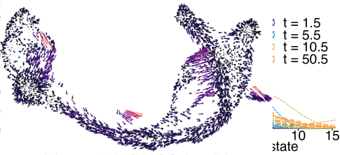
Figure 3: Histograms for the (a) first-passage times and (b) transition-path times obtained by sampling $2048$ trajectories with standard kinetic Monte Carlo (eq. 1) in the Müller-Brown potential, with $N=4225$ and $\alpha_{\text{i}}=A$. (c) Transition paths for a selection of the most-likely trajectories (left) and trajectories visiting the rarest states (right). The colors indicate the states belonging to either of the 3 wells in the Müller-Brown potential. Filled circle indicates the bottom of each well ($U(x,y)=U_{A},U_{B},U_{C}$). The thick dashed line denotes the mean transition path (see appendix C).

This example also emphasizes the difference between first-passage time (FPT) and TPT. To be more quantitative, we considered the non-bridge dynamics described in eq. 1, and we sampled $2048$ trajectories using the Gillespie algorithm. For each trajectory, we defined the last-passage time (LPT) as the time corresponding to the last occurrence of a state belonging to the bottom of well $A$ (filled circles in fig. 3c), and the FPT as the time corresponding to the first occurrence of a state belonging to well $C$. The transition-path time is then simply given by $\text{TPT}=\text{FPT}-\text{LPT}$. We checked that the distribution of the TPT agrees with previously reported theoretical results (figs. S1 and D). Figure 3a-b show that the mean TPT is about 4 orders of magnitude smaller than the mean FPT. Therefore to study the transition $A\to C$ with standard kinetic Monte Carlo, one has to typically simulate trajectories for a duration of time of the order of $10^{4}$ time units, whereas the portion of interest in which the transition $A\to C$ actually happens represents less than $0.01\text{\,}\mathrm{\char 37\relax}$ of the trajectory. Computationnally, such an approach is very inefficient. This emphasizes the benefits of our method, which allows to specifically sample the transition paths. That also means that the value for $t_{\text{f}}$ should be chosen to be slightly larger than the mean TPT.

III.3 Dynamics of differentiation pathways of pancreatic endocrine-cell precursors

We now use our method to generate cell-fate trajectories. We used a mouse pancreatic development dataset [35] which comprises $N=3696$ states (see appendix E). Single cells can be visualized by applying dimensional reduction techniques to the gene expression vectors. In particular, they can be projected onto the first two components obtained by the Uniform Manifold Approximation and Projection method (UMAP) [36, 37], and we computed the transition rates using scVelo (see appendix E). We noted that the resulting rate matrix $\mathbbm{W}$ did not satisfy detailed balance. Using our method, we generated $512$ Markov bridges to study the transition from the ductal cell type to the beta cell type (fig. 4a) and from the ductal cell type to the alpha cell type (fig. 4b). To illustrate how biological insights can be gained, we focus on the differentiation into the alpha cell type. The time-lapse in fig. 5a shows that trajectories spend a variable but significant amount of time in the ductal cell type. This is further corroborated by noting that the average waiting time in the ductal and Ngn3 low-EP cell types are the longest (fig. 5c). Here the waiting time was defined as the time of the last occurrence of a cell type minus the its first occurrence, i.e., $\text{LPT}-\text{FPT}$. Therefore, commitment out of the ductal and Ngn3 low-EP cell types appears to be the main bottleneck of this differentiation route.

Figure 4: Markov bridges for the pancreas dataset, with $N=3696$, $\alpha_{\text{i}}=1103$ (ductal cell type) and $t_{\text{f}}=100$. We study the transition towards the final state (a) $\alpha_{\text{f}}=2379$ (beta cell type) and (b) $\alpha_{\text{f}}=3437$ (alpha cell type). We generated $512$ bridge trajectories in each case. The state coordinates are the first two components of a UMAP analysis.

Once commitment to the Ngn3 high-EP cell type occurs, trajectories move primarily from left to right, with very few jumps in the reverse direction, as qualitatively seen in the time-lapse (fig. 5a). For a more precise statement, we computed for each cell type the mean direction by averaging the curve tangent (velocity normalized to unity, $\mathbf{u}=\mathbf{v}/\|\mathbf{v}\|$) over all states in all trajectories which are in a given cell type. We obtain that the cell types exhibiting the most robust direction are the epsilon, Ngn3 high-EP and pre-endocrine cell types (fig. 5c). While the ductal and Ngn3 low-EP were previously qualified as bottlenecks, these three states should rather be seen as the highways for this differentiation route.

Another insight that can be gained from analyzing bridge trajectories concerns the statistical weights of the different routes for differentiation. In fig. 5b we represented only the part of the trajectories which is between the last occurrence of the Ngn3 high-EP cell type and the first occurrence of the alpha cell type. The trajectories can be broadly divided into three groups, each taking a different route to connect those two cell types. It appears that one of the group is by far the most-likely, containing about $94\text{\,}\mathrm{\char 37\relax}$ of the sampled trajectories. The two other groups have similar weight. Interestingly, it seems that the epsilon cell type is only accessible through these less likely routes. We speculate that this approach can be used to investigate more broadly bifurcations in cell-fate dynamics.

We note that velocities, akin to RNA velocities, can be obtained directly from the transition rates, as:

$$\mathbf{v}_{\alpha}=\sum\limits_{\beta\neq\alpha}(\mathbf{x}_{\beta}-\mathbf{x}_{\alpha})W_{\beta\alpha},$$ (19)

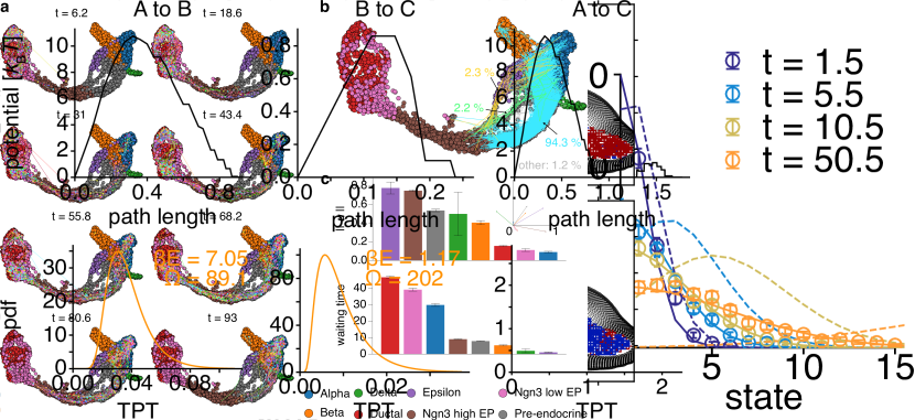
Figure S2: Supplementary figure to fig. 4 of the main text. Velocity field computed as $\mathbf{v}_{\alpha}=\sum_{\beta\neq\alpha}(\mathbf{x}_{\beta}-\mathbf{x}_{\alpha})W_{\beta\alpha}$. Both the lengths and the colors of the arrows scale linearly with $\|\mathbf{v}_{\alpha}\|$.

which seemingly does not require sampling Markov bridges. While the velocity field obtained (fig. S2) is consistent with the observations made above (for example the bottleneck of the ductal/Ngn3 low-EP cell type appears as a region with velocities pointing inward), it is not enough by itself to get a temporal resolution of the dynamics nor to analyze the role of fluctuations such as the statistical weights of different routes, therefore emphasizing the unique type of insights that can be gained by using Markov bridges to study differentiation pathways.

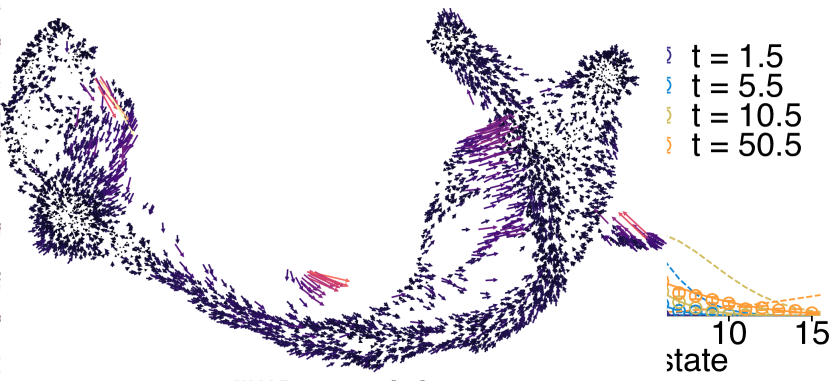
Figure 5: Insights for the differentiation of pancreatic endocrine-cell precursors to alpha cells obtained from the bridge trajectories shown in fig. 4. (a) Time-lapse of the bridge dynamics. Current states are represented with filled circles and the tails show a few of the previous states. (b) Focus on the parts of the bridge trajectories which go from the “Ngn3 high-EP” to “alpha” cell types. (c) Norm of the mean direction ($\|\mathbf{u}\|$) and waiting time ($\text{LPT}-\text{FPT}$) for each cell type. The inset shows the mean direction vector $\mathbf{u}$ for the 8 different cell types.

IV Discussion

The evaluation of the bridge transition rates requires the evaluation of $Q(t)$, which, as already mentioned, involves a matrix exponential (eq. 3). In this work, we have made the choice to use the eigenvalue decomposition of $\mathbbm{W}$ to evaluate $Q(t)$ as shown in eq. 11. However, in general, for any matrix $A=UDU^{-1}$ ($D=\mathrm{Diag}\left(\lambda_{1},\lambda_{2},\ldots,\lambda_{N}\right)$), $\mathrm{e}^{tA}$ is not well approximated (numerically) by $U\mathrm{e}^{D}U^{-1}$ when A is non-normal (see for example [38] and section 11.3 of [39]). Unfortunately, $\mathbbm{W}$ is seldom normal. Therefore, an improvement to our method would be to find more reliable ways to compute $Q(t)$.

Given a system with discrete states, whose dynamics can be described by a master equation as in eq. 1, we have presented a method to generate the subset of possible trajectories that go from one initial state $\alpha_{\text{i}}$ to a final state $\alpha_{\text{f}}$ in a time $t_{\text{f}}$. This method is especially valuable when the final state has a low probability to occur, or when the initial state and the final state are separated by high energy barriers (in the sense of Kramers’ theory). Stochastic realizations of such processes might exhibit a large FPT, and would be sampled with very low efficiency using standard kinetic Monte Carlo methods (e.g. Gillespie algorithm). In such cases, most of the time is therefore spent waiting for a rare event to happen. Yet, in most applications, the sampling of states during this waiting period is of little interest; we are rather interested in the actual transition path once a trajectory has committed to the transition. A benefit of our method is therefore to discard the uninteresting waiting time. This can be done heuristically by adjusting $t_{\text{f}}$ so that it is slightly greater than the typical TPT.

Although we mentioned some lines of improvement, we showed that our approach can be applied in its current state to study diverse phenomena, including cell-fate dynamics, and yield unique insights. The application to scRNA-seq data paves the way for novel computational approaches to study cell development, such as in silico perturbations. We note that it would be interesting to compare results from our methods with experiments tracking cell fate with scRNA-seq and an orthogonal modality (e.g. microscopy), when they become available. Finally, in this work a cell microstate was characterized only through RNA abundance. However it could be enriched with observables coming from other modalities (e.g. morphological measurements coming from microscopy imaging). Provided that an appropriate definition of transition rates is taken, Markov bridges could therefore be used to probe more complex features of cell-fate dynamics.

Appendix A Pseudo code implementations

Algorithm 1 is the implementation we have used in this work to sample Markov bridges. However, as mentioned in the main text, for large systems it might not be adequate due to the computational cost of the eigenvalue decomposition of the $\mathbbm{W}$ matrix. We therefore give algorithm 2, which is an implementation not relying on a matrix decomposition of the form $\mathrm{e}^{t\mathbbm{W}}=U\mathrm{e}^{-tD}U^{-1}$ to evaluate $Q(t)$. In this approach, $Q(t)$ can be evaluated at specified discrete times $t_{j}=j\Delta t$ (with $t_{M}=t_{\text{f}}$) by integrating eq. 2. We note here that matrix-vector multiplications can be performed very quickly with modern GPUs, which can be leveraged in an integration scheme. The time resolution $\Delta t$ should be chosen so that $\Delta t<\Delta t^{\ast}=1/\max_{\alpha}{\left(\Gamma_{\alpha}\right)}$ ($\Gamma_{\alpha}$ is the escape rate as defined in eq. 7).

Algorithm 1 Gillespie sampling for Markov bridges

0:  $(\alpha_{\text{i}},0)$, rate matrix $W$

  Set $(\alpha,t)\leftarrow(\alpha_{\text{i}},0)$

  print  $(\alpha,t)$.

  while $t<t_{\text{f}}$ do

     Draw $u_{1}$ and $u_{2}$ as $\mathcal{U}(0,1)$.

     $\tau\leftarrow$ Solve eq. 10 with $u_{1}$. $Q(t)$ is computed through eq. 11.

     Take $\gamma$ so that $\sum\limits_{\beta=1}^{\gamma-1}V_{\beta\alpha}<u_{2}\Gamma_{\alpha}(t+\tau)\leq\sum\limits_{\beta=1}^{\gamma}V_{\beta\alpha}$.

     Update $(\alpha,t)\leftarrow(\gamma,t+\tau)$.

     print  $(\alpha,t)$.

  end while

Algorithm 2 Standard sampling for Markov bridges

0:  $(\alpha_{\text{i}},0)$, rate matrix $W$, time resolution $\Delta t=t_{\text{f}}/M$

  Integrate eq. 2 and evaluate $Q(t_{j}),\,\forall j\in\llbracket 0,M\rrbracket$.

  Set $(\alpha,t)\leftarrow(\alpha_{\text{i}},0)$

  print  $(\alpha,t)$.

  while $t<t_{\text{f}}$ do

     Draw $u_{1}$ and $u_{2}$ as $\mathcal{U}(0,1)$.

     $\tau\leftarrow j\Delta t$, where $j$ is the smallest integer such that eq. 10 is positive (with $u_{1}$).

     Take $\gamma$ so that $\sum\limits_{\beta=1}^{\gamma-1}V_{\beta\alpha}<u_{2}\Gamma_{\alpha}(t+\tau)\leq\sum\limits_{\beta=1}^{\gamma}V_{\beta\alpha}$.

     Update $(\alpha,t)\leftarrow(\gamma,t+\tau)$.

     print  $(\alpha,t)$.

  end while

Appendix B Analytical treatment of diffusion on the 1D lattice

To solve eq. 14, we introduce the discrete Fourier transform $\tilde{P}_{k}$, such that:

$$\begin{aligned} \tilde{P}_{k}&=\sum\limits_{n=1}^{N}P_{n}\mathrm{e}^{-\mathrm{i}\frac{2\pi}{N}nk},\\ P_{n}&=\frac{1}{N}\sum\limits_{k=1}^{N}\tilde{P}_{k}\mathrm{e}^{\mathrm{i}\frac{2\pi}{N}nk}.\end{aligned}$$ (20)

Taking the time derivative of $\tilde{P}_{k}$, and using eq. 14, we obtain the following system of ODE:

$$\begin{aligned} \frac{\mathrm{d}\tilde{P}_{k}}{\mathrm{d}t}&=-\tilde{\omega}_{k}\tilde{P}_{k},\qquad\forall k\in\llbracket 1,N\rrbracket,\end{aligned}$$ (21)

where we introduced:

$$\begin{aligned} \tilde{\omega}_{k}&=-2\mathrm{i}\sin{\left(\frac{\pi k}{N}\right)}\left(\beta\mathrm{e}^{\mathrm{i}\frac{\pi k}{N}}-\alpha\mathrm{e}^{-\mathrm{i}\frac{\pi k}{N}}\right),\\ \omega_{n}&=(\alpha+\beta)\delta_{n}-\alpha\delta_{n-1}-\beta\delta_{n+1},\end{aligned}$$ (22)

where $\delta_{n}$ is the Kronecker delta. In general, $\tilde{\omega}_{k}$ has a non-zero imaginary part. However, when $\alpha=\beta$, it reduces to $\tilde{\omega}_{k}\leavevmode\nobreak\ =\leavevmode\nobreak\ 4\alpha\sin^{2}{\left(\frac{\pi k}{N}\right)}$.

Equation 21 is straightforwardly integrated and yields:

$$\tilde{P}_{k}(t)=\mathrm{e}^{-\tilde{\omega}_{k}t}\mathrm{e}^{-\mathrm{i}\frac{2\pi}{N}n_{\text{i}}k},$$ (23)

where we used the initial condition $P_{n}(0)=\delta_{n,n_{\text{i}}}$.

For the backward master equation, we introduce $Q_{n}(t)=\mathbbm{P}(n_{\text{f}},t_{\text{f}}|n,t)$. Equation 2 reads:

$$\frac{\mathrm{d}Q_{n}}{\mathrm{d}t}=-\alpha Q_{n+1}-\beta Q_{n-1}+(\alpha+\beta)Q_{n},\qquad\forall n\in\llbracket 1,N\rrbracket,$$ (24)

and its discrete Fourier transform satisfies the ODE:

$$\begin{aligned} \frac{\mathrm{d}\tilde{Q}_{k}}{\mathrm{d}t}&=\tilde{\omega}_{k}^{\ast}\tilde{Q}_{k},\qquad\forall k\in\llbracket 1,N\rrbracket,\end{aligned}$$ (25)

where the superscript $\ast$ denotes complex conjugation. Equation 25 is again straightforwardly integrated and yields:

$$\tilde{Q}_{k}(t)=\mathrm{e}^{-\tilde{\omega}_{k}^{\ast}(t_{\text{f}}-t)}\mathrm{e}^{-\mathrm{i}\frac{2\pi}{N}n_{\text{f}}k},\qquad\forall k\in\llbracket 1,N\rrbracket.$$ (26)

where we used the final condition $Q_{n}(t_{\text{f}})=\delta_{n,n_{\text{f}}}$.

We can now compute the joint probability $R_{n}(t)\leavevmode\nobreak\ \propto\leavevmode\nobreak\ \mathbbm{P}(n_{\text{f}},t_{\text{f}}|n,t)\mathbbm{P}(n,t|n_{\text{i}},0)$:

$$\begin{aligned} R_{n}(t)&=\frac{1}{Z}P_{n}(t)Q_{n}(t),\qquad\forall n\in\llbracket 1,N\rrbracket,\\ \tilde{R}_{k}&=\frac{\tilde{P}\ast\tilde{Q}_{k}}{\tilde{P}\ast\tilde{Q}_{0}},\qquad\forall k\in\llbracket 1,N\rrbracket,\end{aligned}$$ (27)

where $Z=\sum_{n}P_{n}(t)Q_{n}(t)=P_{n_{\text{f}}}(t_{f})=Q_{n_{\text{i}}}(0)$, and $\ast$ in this context is the convolution operator ($U\ast V_{n}=\sum_{m}U_{n-m}V_{m}$). Therefore $R_{n}(t)$ can be exactly computed from eqs. 23, 26 and 27.

By differentiating $R_{n}(t)$ and making use of the forward (eq. 14) and backward (eq. 24) master equations, we obtain the bridge master equation:

$$\begin{aligned} \frac{\mathrm{d}R_{n}}{\mathrm{d}t}&=\alpha\left(\frac{Q_{n}}{Q_{n-1}}R_{n-1}-\frac{Q_{n+1}}{Q_{n}}R_{n}\right)\\ &+\beta\left(\frac{Q_{n}}{Q_{n+1}}R_{n+1}-\frac{Q_{n-1}}{Q_{n}}R_{n}\right),\qquad\forall n\in\llbracket 1,N\rrbracket.\end{aligned}$$ (28)

The bridge master equation eq. 28 has the same form as eq. 6, where the forward and backward rates are now time-dependent:

$$\begin{aligned} V_{n+1,n}=\alpha\frac{Q_{n+1}}{Q_{n}},\qquad V_{n+p,n}=0\quad\text{ if}\quad p>1,\\ V_{n-1,n}=\beta\frac{Q_{n-1}}{Q_{n}},\qquad V_{n-p,n}=0\quad\text{ if}\quad p>1.\end{aligned}$$ (29)

Appendix C Mean and most likely trajectories

The mean trajectory shown in fig. 2 was calculated by averaging trajectories after time registration. First, we defined a suitable subdivision of times $t_{j}=j\Delta t$. For a given trajectory $\{(t_{k},\alpha_{k})\}$, the state at time $t_{j}$, namely $\alpha_{j}$ is such that:

$$\alpha_{j}:=\alpha_{k_{j}},\quad\text{with}\quad t_{k_{j}}\leq t_{j}<t_{k_{j}+1}.$$ (30)

The mean trajectory was obtained by averaging over the coordinates of the $S$ trajectories:

$$\bar{\mathbf{x}}_{j}=\frac{1}{S}\sum\limits_{s=1}^{S}\mathbf{x}_{\alpha_{j}^{(s)}},$$ (31)

where $\mathbf{x}_{\alpha}$ is the coordinates vector associated with state $\alpha$ and $\alpha_{j}^{(s)}$ is the state of trajectory $s$ at time $t_{j}$ after registration as defined in eq. 30.

The mean transition path shown in fig. 3 was obtained by setting the origin of time at the LPT in well A for each trajectory, and then averaging the coordinates as described above.

The most-likely trajectory shown in fig. 2 was obtained by computing the most-likely state $\alpha_{j}^{\mathrm{ML}}$ at each time $t_{j}$:

$$\alpha_{j}^{\mathrm{ML}}=\mathrm{argmax}_{\alpha}\left(\{R_{\alpha}(t_{j})\}\right).$$ (32)

Appendix D Distribution of the transition-path time

We used theoretical results published in [10], investigating the TPT for the symmetric one-dimensional quartic potential. For the overdamped Langevin dynamics, the probability distribution function of the TPT reads:

$$\begin{aligned} p_{\mathrm{TPT}}(t)&=\sqrt{\frac{\beta E}{\pi}}\frac{2\Omega}{1-\mathrm{erf}(\sqrt{\beta E})}\mathrm{e}^{-\Omega t}\left(1-\mathrm{e}^{-\Omega t}\right)^{-\frac{3}{2}}\left(1+\mathrm{e}^{-\Omega t}\right)^{-\frac{1}{2}}\exp{\left(-\beta E\frac{1+\mathrm{e}^{-\Omega t}}{1-\mathrm{e}^{-\Omega t}}\right)},\end{aligned}$$ (33)

where $\beta E$ denotes the height of the potential barrier and $\Omega$ is proportional to the curvature at the top of the potential barrier. The previous equation makes use of the error function:

$$\mathrm{erf}(x)=\frac{2}{\sqrt{\pi}}\int\limits_{0}^{x}\mathrm{d}u\,\mathrm{e}^{-u^{2}}.$$ (34)

The fits shown in fig. S1 were performed by fitting $\beta E$ and $\Omega$ using the Levenberg-Marquardt algorithm.

Appendix E Transition rates for pancreatic cells

We used a mouse pancreatic development dataset [35], and the RNA Velocity method scVelo [27] to obtain a transition matrix. We normalized the raw counts data utilizing the default procedures from scVelo. Each cell is size-normalized to the median of total molecules, and $2000$ top highly variable genes are chosen (with a minimum of $20$ expressed counts for spliced and unspliced mRNA). The scVelo pipeline calculates a nearest neighbor graph using Euclidean distance utilizing $30$ principal components on logarithmic spliced counts, and the mean and variance for each cell its calculated across is 30 nearest neighbors. We give below a Python implementation using the scVelo package (scv), where adata is the annotated pancreas dataset from [35].

scv.pp.filter_genes(adata, min_shared_counts=20)
scv.pp.normalize_per_cell(adata)
scv.pp.filter_genes_dispersion(adata, n_top_genes=2000)
scv.pp.log1p(adata)
scv.pp.moments(adata, n_pcs=30, n_neighbors=30)

We then compute the velocity and transition matrix using scVelo-dynamical. We used the following functions to recover the splicing kinetics of each gene, and the cell-specific latent time which are estimated using expectation-maximization. We computed the transition matrix based on the velocity graph, using the scVelo function with default parameters.

scv.tl.recover_dynamics(adata)
scv.tl.velocity(adata, mode="dynamical")
scv.tl.velocity_graph(adata)
scv.utils.get_transition_matrix(adata, ’velocity’)

Figure S1: Supplementary figure to fig. 3 of the main text. Distribution of the TPT from A to B and from B to C for the Müller-Brown potential. The solid lines denote the fit to the theoretical prediction from [10] (see appendix D).

References

- Shaw et al. [2008] D. E. Shaw, M. M. Deneroff, R. O. Dror, J. S. Kuskin, R. H. Larson, J. K. Salmon, C. Young, B. Batson, K. J. Bowers, J. C. Chao, M. P. Eastwood, J. Gagliardo, J. P. Grossman, C. R. Ho, D. J. Ierardi, I. Kolossváry, J. L. Klepeis, T. Layman, C. McLeavey, M. A. Moraes, R. Mueller, E. C. Priest, Y. Shan, J. Spengler, M. Theobald, B. Towles, and S. C. Wang, Anton, a special-purpose machine for molecular dynamics simulation, Communications of the ACM 51, 91 (2008).
- Elber [2011] R. Elber, Simulations of allosteric transitions, Current Opinion in Structural Biology 21, 167 (2011).
- Cavagna [2009] A. Cavagna, Supercooled liquids for pedestrians, Physics Reports 476, 51 (2009).
- Charbonneau et al. [2023] P. Charbonneau, E. Marinari, G. Parisi, F. Ricci-tersenghi, G. Sicuro, F. Zamponi, and M. Mezard, Spin Glass Theory and Far Beyond: Replica Symmetry Breaking after 40 Years (World Scientific, 2023).
- Shan et al. [2011] Y. Shan, E. T. Kim, M. P. Eastwood, R. O. Dror, M. A. Seeliger, and D. E. Shaw, How Does a Drug Molecule Find Its Target Binding Site?, Journal of the American Chemical Society 133, 9181 (2011).
- Wang et al. [2020] X. Wang, S. Ramírez-Hinestrosa, and D. Frenkel, Using Molecular Simulation to Compute Transport Coefficients of Molecular Gases, The Journal of Physical Chemistry B 124, 7636 (2020).
- Hartmann et al. [2014] C. Hartmann, R. Banisch, M. Sarich, T. Badowski, and C. Schütte, Characterization of Rare Events in Molecular Dynamics, Entropy 16, 350 (2014).
- Hänggi et al. [1990] P. Hänggi, P. Talkner, and M. Borkovec, Reaction-rate theory: fifty years after Kramers, Reviews of Modern Physics 62, 251 (1990).
- Zhang et al. [2007] B. W. Zhang, D. Jasnow, and D. M. Zuckerman, Transition-event durations in one-dimensional activated processes, The Journal of Chemical Physics 126, 074504 (2007).
- Laleman et al. [2017] M. Laleman, E. Carlon, and H. Orland, Transition path time distributions, The Journal of Chemical Physics 147, 214103 (2017).
- Orland [2011] H. Orland, Generating transition paths by Langevin bridges, The Journal of Chemical Physics 134, 174114 (2011).
- Delarue et al. [2017] M. Delarue, P. Koehl, and H. Orland, Ab initio sampling of transition paths by conditioned Langevin dynamics, The Journal of Chemical Physics 147, 152703 (2017).
- Elber et al. [2020] R. Elber, D. E. Makarov, and H. Orland, Molecular kinetics in condensed phases: Theory, simulation, and analysis (John Wiley & Sons, 2020).
- Koehl and Orland [2022] P. Koehl and H. Orland, Sampling constrained stochastic trajectories using Brownian bridges, The Journal of Chemical Physics 157, 054105 (2022).
- Neupane et al. [2012] K. Neupane, D. B. Ritchie, H. Yu, D. A. N. Foster, F. Wang, and M. T. Woodside, Transition Path Times for Nucleic Acid Folding Determined from Energy-Landscape Analysis of Single-Molecule Trajectories, Physical Review Letters 109, 068102 (2012).
- Chung and Eaton [2018] H. S. Chung and W. A. Eaton, Protein folding transition path times from single molecule FRET, Current Opinion in Structural Biology 48, 30 (2018).
- Faccioli et al. [2006] P. Faccioli, M. Sega, F. Pederiva, and H. Orland, Dominant Pathways in Protein Folding, Physical Review Letters 97, 108101 (2006).
- Autieri et al. [2009] E. Autieri, P. Faccioli, M. Sega, F. Pederiva, and H. Orland, Dominant reaction pathways in high-dimensional systems, The Journal of Chemical Physics 130, 064106 (2009).
- Faccioli et al. [2010] P. Faccioli, A. Lonardi, and H. Orland, Dominant reaction pathways in protein folding: A direct validation against molecular dynamics simulations, The Journal of Chemical Physics 133, 045104 (2010).
- McDole et al. [2018] K. McDole, L. Guignard, F. Amat, A. Berger, G. Malandain, L. A. Royer, S. C. Turaga, K. Branson, and P. J. Keller, In Toto Imaging and Reconstruction of Post-Implantation Mouse Development at the Single-Cell Level, Cell 175, 859 (2018).
- Lange et al. [2023] M. Lange et al., Zebrahub – Multimodal Zebrafish Developmental Atlas Reveals the State-Transition Dynamics of Late-Vertebrate Pluripotent Axial Progenitors, bioRxiv , 2023.03.06.531398 (2023).
- Sandberg [2014] R. Sandberg, Entering the era of single-cell transcriptomics in biology and medicine, Nature Methods 11, 22 (2014).
- Gawad et al. [2016] C. Gawad, W. Koh, and S. R. Quake, Single-cell genome sequencing: current state of the science, Nature Reviews Genetics 17, 175 (2016).
- Schaum et al. [2018] N. Schaum et al., Single-cell transcriptomics of 20 mouse organs creates a Tabula Muris, Nature 562, 367 (2018).
- Jones et al. [2022] R. C. Jones et al., The Tabula Sapiens: A multiple-organ, single-cell transcriptomic atlas of humans, Science 10.1126/science.abl4896 (2022).
- La Manno et al. [2018] G. La Manno, R. Soldatov, A. Zeisel, E. Braun, H. Hochgerner, V. Petukhov, K. Lidschreiber, M. E. Kastriti, P. Lönnerberg, A. Furlan, J. Fan, L. E. Borm, Z. Liu, D. van Bruggen, J. Guo, X. He, R. Barker, E. Sundström, G. Castelo-Branco, P. Cramer, I. Adameyko, S. Linnarsson, and P. V. Kharchenko, RNA velocity of single cells, Nature 560, 494 (2018).
- Bergen et al. [2020] V. Bergen, M. Lange, S. Peidli, F. A. Wolf, and F. J. Theis, Generalizing RNA velocity to transient cell states through dynamical modeling, Nature Biotechnology 38, 1408 (2020).
- Lange et al. [2022] M. Lange, V. Bergen, M. Klein, M. Setty, B. Reuter, M. Bakhti, H. Lickert, M. Ansari, J. Schniering, H. B. Schiller, D. Pe’er, and F. J. Theis, CellRank for directed single-cell fate mapping, Nature Methods 19, 159 (2022).
- Weiler et al. [2023] P. Weiler, M. Lange, M. Klein, D. Pe’er, and F. Theis, Unified fate mapping in multiview single-cell data, bioRxiv , 2023 (2023).
- Van Kampen [1992] N. G. Van Kampen, Stochastic processes in physics and chemistry, Vol. 1 (Elsevier, 1992).
- Gillespie [1976] D. T. Gillespie, A general method for numerically simulating the stochastic time evolution of coupled chemical reactions, Journal of Computational Physics 22, 403 (1976).
- Müller and Brown [1979] K. Müller and L. D. Brown, Location of saddle points and minimum energy paths by a constrained simplex optimization procedure, Theoretica chimica acta 53, 75 (1979).
- Müller [1980] K. Müller, Reaction Paths on Multidimensional Energy Hypersurfaces, Angewandte Chemie International Edition in English 19, 1 (1980).
- Binder et al. [1992] K. Binder, D. W. Heermann, and K. Binder, Monte Carlo simulation in statistical physics, Vol. 8 (Springer, 1992).
- Bastidas-Ponce et al. [2019] A. Bastidas-Ponce, S. Tritschler, L. Dony, K. Scheibner, M. Tarquis-Medina, C. Salinno, S. Schirge, I. Burtscher, A. Böttcher, F. J. Theis, H. Lickert, and M. Bakhti, Comprehensive single cell mRNA profiling reveals a detailed roadmap for pancreatic endocrinogenesis, Development 146, dev173849 (2019).
- McInnes et al. [2018] L. McInnes, J. Healy, and J. Melville, UMAP: Uniform Manifold Approximation and Projection for Dimension Reduction, arXiv , 1802.0342 (2018).
- Becht et al. [2019] E. Becht, L. McInnes, J. Healy, C.-A. Dutertre, I. W. H. Kwok, L. G. Ng, F. Ginhoux, and E. W. Newell, Dimensionality reduction for visualizing single-cell data using UMAP, Nature Biotechnology 37, 38 (2019).
- Moler and Van Loan [2003] C. Moler and C. Van Loan, Nineteen dubious ways to compute the exponential of a matrix, twenty-five years later, SIAM review 45, 3 (2003).
- Golub and Van Loan [2013] G. H. Golub and C. F. Van Loan, Matrix computations (JHU press, 2013).