MotherNet: A Foundational Hypernetwork for Tabular Classification

Abstract

The advent of Foundation Models is transforming machine learning across many modalities (e.g., language, images, videos) with prompt engineering replacing training in many settings. Recent work on tabular data (e.g., TabPFN) hints at a similar opportunity to build Foundation Models for classification for numerical data. In this paper, we go one step further and propose a hypernetwork architecture that we call MotherNet, trained on millions of classification tasks, that, once prompted with a never-seen-before training set generates the weights of a trained “child” neural-network. Like other Foundation Models, MotherNet replaces training on specific datasets with in-context learning through a single forward pass. In contrast to existing hypernetworks that were either task-specific or trained for relatively constraint multi-task settings, MotherNet is trained to generate networks to perform multiclass classification on arbitrary tabular datasets without any dataset specific gradient descent.

The child network generated by MotherNet using in-context learning outperforms neural networks trained using gradient descent on small datasets, and is competitive with predictions by TabPFN and standard ML methods like Gradient Boosting. Unlike a direct application of transformer models like TabPFN, MotherNet generated networks are highly efficient at inference time. This methodology opens up a new approach to building predictive models on tabular data that is both efficient and robust, without any dataset-specific training.

1 Introduction

Foundation Models, i.e., large transformer-based (Vaswani et al., 2017) models trained on massive corpora, are disrupting machine learning in many areas such as natural language and reasoning tasks. The field is quickly moving from small task-specific models to large generic models with task-specific instructions via prompting and in-context learning.

This tidal wave of change has yet to reach tabular data, the most common data type in real-world machine learning applications (Chui et al., 2018), where currently traditional machine learning methods are still the norm. In this paper, we explore a new angle of applying transformer-based Foundational Models to tabular classification. Such models have the potential to transform ML for Tabular data, replacing costly and slow AutoML activities with in-context learning. The existing TabPFN approache, while very promising in terms of accuracy, fall short of state-of-the-art classical solutions in terms of scalability to large training datasets and inference runtime. We focus our attention towards removing these limitations.

We introduce a new architecture, called MotherNet, which adapts the TabPFN transformer architecture (Hollmann et al., 2022; Vaswani et al., 2017) to produce model weights for a neural network of fixed structure (a two hidden layer neural network in the experiments ) that performs competitively with baseline methods such as gradient boosting (Friedman, 2001; Chen & Guestrin, 2016). Using MotherNet to generate neural network weights substantially outperforms learning by gradient descent in computational efficiency, accuracy and ease of use on small tabular datasets.

Our approach combines the transformer architecture of TabPFN (Hollmann et al., 2022) with the idea of hyper-networks (Ha et al., 2017), to produce state-of-the-art classification models in a single forward pass. Unlike original work in hypernetworks (Ha et al., 2017), which used a small hyper network to generate a large “main” network, we are training a large, transformer-style hyper-network to generate a compact classification network. Compared to the approach of Hollmann et al. (2022), this allows for very fast inference, making the model applicable for low-latency requirements and for prediction on large datasets. Compared to earlier work on hypernetworks, we train a single hyper-network to address tabular classification on numeric data in general, i.e. in style of a foundational model, instead of a task-specific or multi-task hypernetwork.

Our key contribution is demonstrating that it is indeed possible to generate neural networks directly as the output of a transformer model, without the need to do any dataset-specific learning or gradient descent. Using a fixed model structure, we are able to produce neural networks that work well on small numeric tabular datasets from the OpenML CC-18 benchmark suite (Bischl et al., 2017).

The key intuition is that the “mother” network has been trained on millions of classification scenarios and has learned a certain degree of regularization. This “wisdom” is passed down to the child, allowing for the child to operate in a label-scarce environment without over-reacting to outliers present in the prompt.

Aside from applications to AutoML, our approach also has an interesting theoretical angle. Given a tabular training dataset, MotherNet learns (via in-context learning) to build a machine learning model in the form of an MLP. However, throughout the procedure, there is no optimization for training set accuracy at any point. Therefore, the MotherNet approach does not use framework of regularized empirical risk minimization that is the basis of nearly all modern machine learning methods. Instead, it directly optimizes expected test-set performance, with distributional assumptions encoded in the training of the MotherNet model.

Our findings can be summarized as follows:

• It is possible to create accurate small neural networks without gradient descent, using in-context learning with a transformer.

• Our approach performs competitively with baseline methods, including Gradient Boosting with hyper-parameter tuning, without any dataset specific tuning of our method.

• Our approach has extremely fast inference time, as well as combined inference and training time.

• Our approach provides a proof-of-concept for building standard machine learning models without relying on empirical risk minimization, therefore providing a new perspective on generalization.

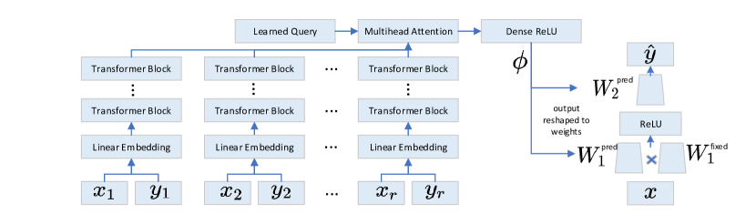
Figure 1: MotherNet architecture. Given training data $(x_{1},y_{1}),\dots,(x_{r},y_{r})$, the transformer produces a vector $\phi$, which is reshaped to weight matrices of an MLP with low-rank weight structure.

2 Related Work

2.1 Foundation Models

The use of Foundation Models for natural language tasks has taken research and applications by storm, especially since the launch of ChatGPT and GPT-4 (OpenAI, 2023). One of the surprising observations about the work in this area is that models trained purely for next word prediction can be adapted to novel NLP tasks by providing the correct prompt (Brown et al., 2020). This approach replaces training or even fine-tuning by providing task-dependent input to a fixed model, also known as in-context learning. While the original training of the model might be quite expensive (computationally, data needed, and financially), once the model is built, in-context learning allows for near-instantaneous adaptation to new tasks and new contexts. Much work has been done to further improve the responsiveness to prompts, and adjust output to human preference. Our paper addresses tabular numeric data, and in this context, providing task definitions as part of the input is non-trivial. Therefore we fix the task to multi-class classification. Our goal is to produce a Foundation Model that can generalize this task across training datasets, in contrast to state-of-the-art approaches that train a classifier per dataset.

2.2 Transformers for Tabular Data

There have been several works investigating the use of small, heterogeneous tables for question answering, and extracting tables from data, using large language models and specifically fine-tuned transformers (Yin et al., 2020; Iida et al., 2021).

While generic language models can be adapted to work on tables, the restriction on the number of input tokens, even for the largest models, severely limits the amount of data that can be ingested. Using a dedicated architecture for numeric data allows scaling to much larger datasets. More specifically, compare the memory usage of a large language model like LLAMA (Touvron et al., 2023) with that of a transformer for numeric data such as TabPFN (Hollmann et al., 2022). LLAMA has a vocabulary size of 32,000 and an embedding dimension of 4096 (in the smallest version). Expressing a single feature in the iris dataset, which are decimals with two places, takes four tokens, so approximately $4096\cdot 4=16384$ floating point numbers or a sparse vector of length $32,000\cdot 4=128000$. Using a transformer for floating point tables, it takes a single floating point number. Expressing the whole iris dataset (four features, three classes, 150 data points) in a way consumable by a large language model yields 5000 to 15000 tokens, depending on the tokenizer and JSON representation, which is above the capability of most large language models: Llama supports 2048, the largest current model, GPT-4, up to 32k, while Hollmann et al. (2022) showed scaling to 100 features and 1000 data points (up to 5000 in extrapolation experiments). Notably, the token limits on the Large Language Model combine input, output and instructions, while the limitations in Hollmann et al. (2022) are for the training set, with the assumption of a test set of the same size.

2.3 TabPFN

Recently Hollmann et al. (2022), building on the work of Müller et al. (2021), introduced a transformer architecture that is capable of performing supervised classification on tabular numeric data. This work is quite distinct from other transformer architectures on tabular data in that it is focused on numeric input and numeric output. The authors design a prior over synthetically generated datasets, based on Structural Causal models and Bayesian Neural Networks. Using draws from this prior, they are able to train a model that generalizes to perform supervised classification on real-world tabular datasets. Our work builds on the work of Hollmann et al. (2022), and adds the capability to create a dataset-specific model. This allows much faster and more memory-efficient inference given a fixed training set, and allows standard model inspection techniques for neural networks, as opposed to inspecting the activations of the transformer model. We use the prior of Müller et al. (2021), therefore sharing their assumptions about the data distribution, and as we are using a transformer architecture, we are also limited in the training set size similar to their approach.

2.4 Learning to Learn and Meta-learning

There has been a long history of approaches to “learning to learn” and to build neural network that produce other neural networks in machine learning (Schmidhuber, 1992; Ravi & Larochelle, 2016; Andrychowicz et al., 2016; Thrun & Pratt, 1998). Given the long history, we will only review some more recent and closely related approaches.

Ha et al. (2017) introduce the term hypernetwork for networks that produce networks using task-specific embeddings. The hypernetwork and embedding are both learned via gradient descent on the same dataset, reducing the approach (in the non-recurrent case) in essence to a standard neural network with a low-rank structure in the weights.

Later, Finn et al. (2017) proposed the MAML framework for multi-task learning, which generates “easy-to-finetune” weights for a fixed architecture, which allows quick adaption to new tasks. Among the many follow-ups to MAML, of particular relevance to this work is CAVIA (Zintgraf et al., 2019), which decomposes the network into a task-specific part to be fine-tuned in the ”inner loop” and a task agnostic part, which is fixed after meta-learning. This approach has been studied more in-depth, and put into the context of hypernetworks in Zhao et al. (2020). Zhao et al. (2020) learn an initialization for the task embedding using a MAML-style objective, which can then be further fine-tuned using gradient descent.

Similar to our work, MAML and later variants aim to speed up and improve learning of a network by meta-learning from a related set of tasks, using a fixed network architecture. However, MAML requires performing gradient descent to adjust to specific tasks, and factorization based approaches like Zintgraf et al. (2019) and Zhao et al. (2020) still require gradient descent on the task-specific components of the model, while MotherNet produces task-specific weights using a HyperNetwork, requiring no further gradient descent. Furthermore, MAML and related multi-task methods have usually been applied to tasks that require large models, in particular computer vision tasks, with close relationships between tasks, i.e. learning new classes in an image classification dataset.

Not relying on gradient descent not only provides improved computational performance, but it fundamentally changes the nature of the optimization. In CAVIA and MAML-style approaches, the network weights are (directly or indirectly) optimized to minimize training-set loss on a new task, while MotherNet never optimizes training-set loss, and so does not suffer from overfitting (though potentially from meta-overfitting to the meta-trainingset). This removes the need for any regularization for generating the task-specific model.

While it would be possible to adapt MAML to the setting of variable number of features and classes by borrowing methods from Hollmann et al. (2022), this is beyond the scope of this work.

More closely aligned with our work, Bertinetto et al. (2016) also propose a gradient-free approach to produce fully-fledge student networks based on single-shot examples in OCR and object tracking. Their objective and formulation closely resembles ours; however, in this work, a single “exemplar” is a tabular training dataset, while in Bertinetto et al. (2016), it is a single handwritten digit, or example of an object to track. By learning to ingest generic tabular datasets, our approach successfully deals with a much broader variety of tasks.

In spirit, our approach is also related to more classical meta-learning approaches, that have attempted at generalizing knowledge among datasets  (Vanschoren, 2018). For tabular data, this has usually been in the form of hyper-parameters, either via the generation of portfolios (Brazdil et al., 2003; Wistuba et al., 2015; Abdulrahman et al., 2018) or by using dataset characteristics such as meta-features (Rivolli et al., 2018). Our work differs, in that our meta model takes in the whole dataset, and, instead of producing hyper-parameters or candidate model architectures, it directly produces a fully trained model. This makes the MotherNet architecture much cheaper than traditional meta-learning approaches, in that no actual per-dataset model training needs to be performed in the meta-training or prediction phases. Commonly, meta-learning also requires local search over hyper-parameters, in addition to the use of a meta-model (Hutter et al., 2019), while we found our one-shot weights to work robustly without any modifications.

3 Methodology

3.1 Background

Hollmann et al. (2022) introduced TabPFN, an adaption of the transformer architecture to solve tabular classification problems. TabPFN uses a transformer where each input “token” is a row of the tabular dataset. The model is adapted to work with a variable number of features by zero-padding (and scaling) to 100 features. For the training data, linear projections of the input rows are summed with linear projections of integer classification labels. For the test data, the addition of labels is simply omitted, and class-probabilities are produced as output tokens. The model is trained to minimize cross-entropy of probabilistic predictions on the test data points. Attention is masked so that all training points can attend to all other training points, while test points can only attend to training points. A variable number of classes is handled by training for up to ten classes, and when predicting for a dataset with $k\leq 10$ classes, using only the first $k$ outputs in the softmax layer.

TabPFN showed strong predictive performance without any per-dataset tuning, and with extremely fast time to train and predict on small datasets ($\leq 2000$ data points). Because of the quadratic nature of the self-attention matrix, training on larger datasets is impractical with the method proposed in Hollmann et al. (2022). Their prior focused on numeric-only data, so their model was evaluated on datasets without categorical or missing features. We extend this approach in our work removing some of the limitations discussed next.

Limitations of TabPFN

Comparing speed and computational efficiency between TabPFN and traditional ML and AutoML methods is somewhat complicated, as they have very different characteristics. In particular, there is no dataset specific training phase after meta-training when applying TabPFN, only near-instantaneous in-context learning. Prediction, on the other hand, is significantly slower than prediction in standard ML models, as predicting on $N_{p}$ data points given a training dataset of size $N_{t}$ requires constructing attention matrices of sizes $N_{t}\times N_{t}$ and $N_{t}\times N_{p}$. This is similar to the characteristics of traditional $kNN$ classifiers or Gaussian Process models, which (absent specific optimizing data structures) have no training phase.

The gold standard of modern tabular learning, gradient boosted trees (Friedman, 2001; Chen & Guestrin, 2016; Ke et al., 2017), on the other hand, has significant training cost, in particular when accounting for hyper-parameter tuning, but has prediction cost independent of the training set size, and only dependent on the model size.

From these, it is clear that applying TabPFN to large training sets using the standard transformer architecture is challenging. Moreover, when looking at just prediction time, TabPFN is far behind gradient boosted models.

While both models have prediction time linear in the number of test data points $N_{t}$, the constant in the case of TabPFN is much larger. Together with the memory requirements of a large transformer model, this makes TabPFN impractical for settings where fast, on-demand predictions are required.

Next we present two approaches, a surprisingly effective baseline distillation approach, and MotherNet, that address some of the runtime and scalability limitations of TabPFN.

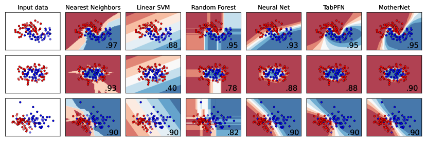
Figure 2: Comparing decision boundaries on synthetic toy datasets, adapted from the scikit-learn (Pedregosa et al., 2011) documentation. MotherNet decision boundaries closely resemble TabPFN and traditional Neural Network boundaries.

3.2 Distillation

While TabPFN has good training-time properties, it has high prediction time cost. A natural solution is to create a dataset specific compression or instantiation of the model based on a given training dataset. There are many potential routes to this, including model pruning or distilling the transformer model. We chose to evaluate a simple baseline, applying the predictions of TabPFN as a teacher model for a small feed-forward neural network, such as a Multilayer Perceptron (MLP) model, that is trained specifically for a dataset, analogous to the methodology of Hinton et al. (2015). Note that we are not attempting to distill TabPFN, but instead create dataset-specific distillations for each dataset we want to predict on. Furthermore, while TabPFN is acting as a teacher model, it never saw the dataset for which it is a teacher during training time. While this is a natural way to distill the model for dataset-specific prediction, we are not aware of this being investigated before. The reduction in model size and complexity between the original model and the distilled model is dramatic (at nearly 3 orders of magnitude): We use an MLP model with two hidden layers of size 128, which results in a maximum of  30k parameters (with 100 input features and 10 targets, i.e., the limit in the datasets we consider as most datasets are smaller), while the original TabPFN has  26M parameters.

In Section 4.2 we show that this distillation process is extremely effective in approximating the predictions made by by the original model without any dataset-specific tuning of the MLP hyper-parameters. This is in stark contrast to training the same MLP from scratch using gradient descent, which is unable to achieve competitive results without hyper-parameter tuning. Creating the distilled model introduces a distinct training phase in using TabPFN, but tremendously accelerates prediction.

Next we present a novel approach that also produces a small ”child” network, without incurring the cost of a distinct training phase.

3.3 MotherNet: Generating Model Weights

Motivated by the success of TabPFN, and inspired by previous work on hypernetworks, we propose MotherNet, a transformer architecture that is trained to produce machine learning models with trained weights in a single forward pass. This methodology combines the benefits of a Foundation Model that does not require dataset specific training or tuning with the high efficiency of a compact model at inference time. The resulting models are small feed-forward neural networks (an MLP with two hidden layers of size 512 in our experiments), that have competitive performance, created without the use of back-propagation or any loss minimization on the training set. The training process of the overall architecture can be described as:

$$\begin{split}\min_{\theta}\sum_{i}\mathcal{L}(\texttt{MLP}_{\phi},D^{p}_{i}),\\ \textrm{ where }\phi=\texttt{MotherNet}(\mathbf{D^{t}_{i}},\theta))\end{split}$$ (1)

Where $\theta$ are the parameters of the MotherNet transformer, $D^{t}_{i}$ and $D^{p}_{i}$ are training and prediction portion of synthetic dataset $i$, $\textrm{MLP}_{\phi}$ is the feed-forward neural network with parameters given by $\phi$ and $\mathcal{L}(M,D)$ is the cross entropy loss of the model $M$ evaluated on datasets $D$. Training is performed by back-propagation through the whole architecture (from the output of the child model, and through the transformer layers) where each training sample corresponds to one dataset. We will refer to this process as meta-training in the following. During meta-training, the parameters $\theta$ are learned using synthetic datasets, using the prior from Hollmann et al. (2022) and then frozen (as common in Foundation Models). To apply the model to a new (real) dataset $\hat{D}$ consisting of a training portion $\hat{D}^{t}$ and a prediction portion $\hat{D}^{p}$, we evaluate $\texttt{MotherNet}(\hat{D}^{t},\theta)$, which produces a vector of parameters $\hat{\phi}$. This vector is then used as the weight and bias vectors of a feed-forward neural network (properly reshaped), which can be used to make predictions on $\hat{D}^{p}$. We refer to this approach of applying MotherNet to create a child network as in-context learning. This approach is somewhat similar to the approach of Zintgraf et al. (2019), however instead of producing initializations that have to be fine-tuned on a specific dataset, we directly produce the final weights of the model. The absence of gradient descent in our method not only provides an advantage in terms of runtime complexity, it also eliminates the need to apply any regularization, as the model was trained for generalization, not training set performance.

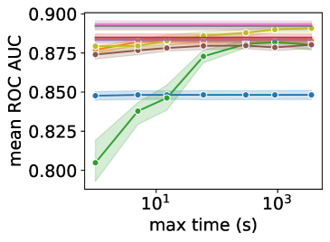
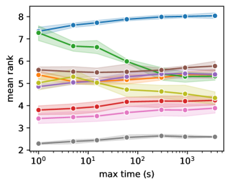
Figure 3: Comparison of TabPFN, MLP-distill and MotherNet with tuned baselines on the test datasets. Left: Mean normalized ROC AUC over time. The two versions of TabPFN overlap too closely to be distinguished. Right: Mean rank over time. Predictions of transformer-based models are constant over the $x$ axis. Compare Figure 9 for validation set results. All transformer based methods use an ensemble of of size 3.

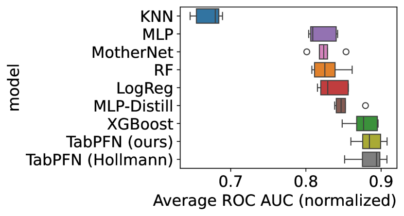
Figure 4: Comparison of normalized mean ROC AUC on test datasets, based on tuning baselines for 1h.

The success of our approach might inspire some skepticism, but we believe our empirical results show not only the feasibility but the competitiveness of the method.

An overview of the model architecture is shown in Figure 1. MotherNet maintains the structure of input encoding and twelve transformer layers of TabPFN on the training set, which produces activations of size $m$ (512 for the experiments) for each pair of training data point and label. On top of this, another attention layer is added, that, based on a learned query vector, reduces all activations to a single dataset embedding $E$ of size $m_{\textrm{all}}$ (2048 in the experiments). The query token is learned during gradient descent and then fixed, similar to prefix tuning (Li & Liang, 2021), but present only in an attention module on top of the transformer layers, not in every layer of the network.

This embedding $E$ is then decoded into the vector $\phi$ using a one-hidden-layer feed-forward neural network. The vector $\phi$ of activations based on the transformer is then reshaped into weights and biases for another feed-forward network.

Initial experiments showed this approach to be very successful, but lead to very large transformer models as a function of the size of the network that was to be produced. Therefore, we employed a standard compression technique and imposed a low rank structure on the weights of the produces networks. As in Ha et al. (2017) we decompose the weights into two components, $W_{i}^{\text{pred}}$ that is the output of the transformer, and $W_{i}^{\text{fixed}}$ that is learned during the meta-training phase and fixed during in-context learning.

The low-rank structure drastically reduces the number of entries in $\phi$ for a given size of neural network produces. All our experiments use the low-rank version, which yielded slightly better AUC on the validation set, at a much smaller model size.

Prediction with MotherNet

For prediction, given a dataset $D^{t}$ with $r$ features and $c$ classes, and output $\phi=\texttt{MotherNet}(\mathbf{D^{t}_{i}},\theta)$, we discard all but the first $r$ rows of the input layer matrix, and keep only the first $c$ columns of the output matrix (which produces up to 10 classes, of which only the first $c$ are used) in the output network $\texttt{MLP}_{\phi}$, resulting in a network with an input layer of size $r$, hidden layers of size 512 and an output layer of size $c$.

We found that ensembling improves predictive performance, as was found by Hollmann et al. (2022). We use the same ensembling strategy as used there, which includes circular permutations of features and classes, and optional encoding using Yeo-Johnson encoding (Yeo & Johnson, 2000). This results in $r\cdot c\cdot 2$ possible combinations of permutations and transformation, of which we sample 3 for all our experiments, following the default setting of Hollmann et al. (2022). Sampling a larger number improves performance but slows down both training and predictions. The predictions that are produced, both by individual networks, and the ensemble, are quite smooth and similar to traditionally learned neural networks or TabPFN, see Figure 2.

did	name	d	n	k
11	balance-scale	5	625	3
14	mfeat-fourier	77	2000	10
15	breast-w	10	699	2
16	mfeat-karhunen	65	2000	10
18	mfeat-morphological	7	2000	10
22	mfeat-zernike	48	2000	10
23	cmc	10	1473	3
29	credit-approval	16	690	2
31	credit-g	21	1000	2
37	diabetes	9	768	2
50	tic-tac-toe	10	958	2
54	vehicle	19	846	4
188	eucalyptus	20	736	5
458	analcatdata_authorship	71	841	4
469	analcatdata_dmft	5	797	6
1049	pc4	38	1458	2
1050	pc3	38	1563	2
1063	kc2	22	522	2
1068	pc1	22	1109	2
1462	banknote-authentication	5	1372	2
1464	blood-transfusion-…	5	748	2
1480	ilpd	11	583	2
1494	qsar-biodeg	42	1055	2
1510	wdbc	31	569	2
6332	cylinder-bands	40	540	2
23381	dresses-sales	13	500	2
40966	MiceProtein	82	1080	8
40975	car	7	1728	4
40982	steel-plates-fault	28	1941	7
40994	climate-model-…	21	540	2

Table 1: Test dataset names and properties, taken from Hollmann et al. (2022). Here did is the OpenML Dataset ID, d the number of features, n the number of instances, and k the number of classes in each dataset.

Training MotherNet

We train MotherNet using the setup of Hollmann et al. (2022) with one modification. Instead of using a linear embedding of integer class encodings, we use a one-hot encoding of classes. We train the network on a single A100 GPU with 80GB of GPU memory, which takes approximately four weeks. We found that training MotherNet from scratch using the objective in 1 is possible, but warm-starting by initiating the transformer using the TabPFN weights can accelerate training. We are using increasing batch sizes of 8, 16 and 32 and a learning rate of 0.00003, with cosine annealing (Loshchilov & Hutter, 2016). We fix the output architecture to an MLP with two hidden layers with 512 hidden units each, and with weight-matrices of rank 32. We evaluated variants of the architecture hyper-parameters on the validation set of Hollmann et al. (2022). The best-performing version of our architecture has 149M parameters, with 124M of these in the decoder attached to the last transformer. Somewhat surprisingly, we found that a decoder with a learned embedding $E$ of size 2048 (see Figure 1), and a hidden dense hidden layer of size 4096 for decoding works well. This is particularly surprising because it means the whole training dataset is first compressed to a vector of length 2048, and then expanded into a vector of size $25738$ to encode the low-rank components of the weights for the network that is produced. We suspect that this choice of architecture is not optimal, and better performance could be achieved with longer training and larger embedding dimensions, or similar performance could potentially be achieved by producing smaller neural networks.

Training TabPFN

We trained our own version of TabPFN to compare it to the version provided by Hollmann et al. (2022). We made the same architectural change for encoding the labels as described for MotherNet above. As for MotherNet, we used a single A100 GPU with 80 GB of GPU memory. We used a batch-size progressively increasing from 32 to 128, and a learning rate of $0.0001$ with cosine annealing. We train for ca 4.4M steps, which means our model saw ca 200M synthetic datasets, compared to the ca 10M synthetic datasets for the original TabPFN.

4 Experimental Evaluation

We follow the experimental evaluation of Hollmann et al. (2022), leveraging their synthetic dataset generation and evaluation methodology.

4.1 Evaluation Protocol

We focus our evaluation on the 30 datasets within the CC-18 with less than 2000 samples, listed in Table 1, and compare models using one-vs-rest ROC AUC. When aggregating across datasets, normalize scores with the minimum and maximum performance achieved on the dataset by any algorithm. As in Hollmann et al. (2022), we split each dataset 50/50 into training (i.e. per-dataset model generation via in-context learning) and test set, and repeat this split five times. We refer to that work for an in-depth comparison of TabPFN with current AutoML methods. Here, we compare predictive performance and runtime of the following models: TabPFN as provided by the authors of Hollmann et al. (2022), our own version of TabPFN, MLP-distill, MotherNet, a vanilla MLP, and baselines consisting of Histogram Gradient Boosting (Chen & Guestrin, 2016; Friedman, 2001), $k$-Nearest Neighbors, Logistic Regression and Random Forests (Breiman, 2001). In contrast to Hollmann et al. (2022), we include datasets which contain categorical features or missing values; we use a one-hot-encoding for categorical values and fill missing values with zeros as in Hollmann et al. (2022).

There is no dataset specific tuning for any of the transformer architectures , while for the other methods we vary the maximum time used for tuning hyper-parameters.

4.2 Results

The results are shown in Figure 3 and Figure 4. Error bars show standard deviation over the five splits of each dataset. Figure 5 shows the Critical Difference Diagram (Demšar, 2006) for the different models given 60 minutes of tuning (furthest right point Figure 3). We can see that TabPFN outperforms all other methods, even at 60 minutes of tuning. There is a substantial gap between the original TabPFN and our version, likely because of the larger training budget. While the distilled version MLP-distill does not achieve the same level of performance, it outperforms all the baseline models in rank, eventhough baseline models include tuning. This is particularly noteworthy since we did not perform any per-dataset tuning of the student network. It seems the probabilistic predictions produced by TabPFN provide enough regularization for good generalization.

Our MotherNet approach performs comparatively to the baseline methods on the test set until 1 minute of tuning time, when it is overtaken by XGBoost (Chen & Guestrin, 2016). We found that on the validation set, MotherNet outperforms XGBoost until 60 minutes of per-dataset training (see Figure 9). Interestingly, the MLP which is trained using standard gradient descent is performing much worse than MLP-distill and worse than MotherNet until about 5 minutes of per-dataset tuning for the test datasets. On the validation set, MotherNet outperforms the MLP even after 1h of tuning, Figure 9, Figure LABEL:fig:validation_set_cd. Clearly MotherNet provides a feasible alternative to training with gradient descent on these datasets.

Table 2 compares average per-dataset speed-ups (higher is better) for different modeling phases with XGBoost as a baseline. If we only consider prediction time, TabPFN is about five times slower than XGBoost, while MotherNet on the GPU is about four times faster than XGBoost. This is the main advantage we look to gain from using MotherNet over TabPFN. However, MLP-distill is even faster, at 21 times the prediction speed of XGBoost on average, likely due to the ensembling described in Section 3.3. However, if we look at the speed of training (assuming optimum hyper-parameters are known) and prediction, which is particularly critical for model development, we see that MotherNet on GPU provides a 36x speedup over XGBoost, while MLP-distill only obtains parity.

In most real-world settings, hyper-parameters are unknown, and Table 2 shows the substantial speed-up that can be achieved using one of the foundational models. Using TabPFN or MotherNet on the GPU results in more than 300x speedup for model-development, while MotherNet on the CPU still provides 7x speedup. We want to point out that these speedup figures might depend strongly on the tuning time estimated for XGBoost. On the test dataset, XGBoost achieves parity with MotherNet after 30 seconds of tuning, while on the validation set, it takes one hour; this means speed-ups on the validation set are two orders of magnitude larger than on the test set. This points at a practical difficulty of tuning parameters: in practice it is often unclear how much time should be allocated for hyper-parameter tuning. Using MotherNet removes this trade-off by providing competitive accuracy near-instantaneously without any tuning.

From Figure 5 and Figure 3 we can see that MLP-distill outperforms MotherNet in terms of ROC AUC on the test datasets, while the same is not true on the validation datasets, see Figure 8 and Figure 9. Understanding the differences in performance between MLP-distill and MotherNet on these datasets is an interesting question that we leave for future work. Some qualitative results on the test set are shown in Figure 7.

	predict	fit+predict	fit+predict
			+ tuning
model
XGBoost	1.00	1.00	1.00
LogReg	98.89	201.14	2.33
MLP	13.64	1.51	0.12
RF	0.85	22.05	0.01
TabPFN GPU	0.18	40.45	310.16
MLP-Distill GPU	21.27	1.03	7.63
MotherNet CPU	2.68	1.01	7.00
MotherNet GPU	4.28	36.29	335.43

Table 2: Speedup of various modeling phases over XGBoost. We omitted KNN since it does not perform competitively with the other approaches.

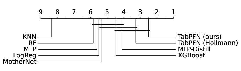
Figure 5: Critical Differences Diagram (Demšar, 2006) of TabPFN, MLP-distill and MotherNet with tuned baselines over the test datasets of Hollmann et al. (2022), listed in Table 1.

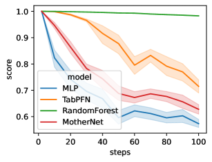
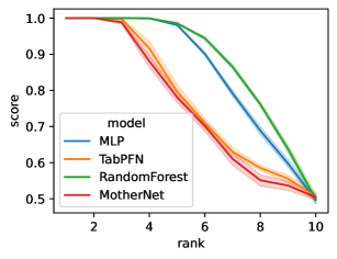
Figure 6: Mean test-set accuracy on synthetic binary classification datasets comparing TabPFN and MotherNet to untuned variants of scikit-learn classifiers. Left: one-dimensional dataset with variable number of jumps. Right: boolean functions of varying rank.

5 Failure Cases of TabPFN and MotherNet

When examining validation test results (see Appendix B), we found that there was, unsurprisingly, a strong correlation between MotherNet and TabPFN results, and both under-performed compared to the tuned XGBoost on the same datasets, in particularly parity5_plus_5, teachingAssitant and schizo. When looking at these dataset in more detail, we found that there was data leakage in both teachingAssitant and schizo datasets via an ID column, see Appendix D for details. While in these particular cases, the datasets could be considered faulty, there was information included in the data that a tree-based model was able to exploit, while TabPFN and MotherNet could not; in this case discontinuous functions with many jumps in a single continuous feature. The parity5_plus_5 illustrated a different failure case: this dataset relies on matching boolean patterns on a subset of the columns. While (Hollmann et al., 2022) showed that irrelevant features degrade the performance of TabPFN, removing the irrelevant features did not improve performance on parity5_plus_5; the issues rather seems in the inability of TabPFN and MotherNet to memorize binary patterns. Based on these two failure cases, we generated families of synthetic functions to illustrate the shortcomings. We compare TabPFN and MotherNet to two simple baselines, RandomForestClassifier and MLPClassifier from scikit-learn (Pedregosa et al., 2011) with default parameters without tuning, see Appendix C for details. Figure 6 shows that as the complexity of the dataset increases, either in terms of jumps in a 1d function, or in terms of complexity of a boolean function, TabPFN and MotherNet degrade in performance much more quickly than the Random Forest model. The MLP is able to easily learn the boolean datasets, but not the discontinuous 1d datasets; somewhat suprisingly, given the underperformance of MotherNet on this task, MotherNet slightly outperforms the MLP. We speculate that these failure cases can be addressed in future work by including similar synthetic datasets in the prior. It might also be necessary to adopt the architecture of MotherNet, for example using fourier features (Tancik et al., 2020) to account for discontinuities.

6 Conclusion

We demonstrated that it is possible to achieve competitive results on small numeric tabular datasets by producing neural networks using a single forward pass in our MotherNet architecture, without using gradient descent. We also find that distilling TabPFN, into a small neural network is highly effective and doesn’t require dataset-specific hyper-parameter tuning — as opposed to training a similar neural network from scratch. The distilled network performs somewhat better than the network produced in a forward pass with our current architecture for MotherNet, though this result is not consitent between training and validation datasets; importantly, networks generated via distillation are substantially slower to produce. The fact that a model can be generated with a simple forward pass is quite surprising, and our work should be seen as a first exploration into this idea.

Open Questions and Future Work

Possibly the most interesting open question from a theoretical perspective is “Why does this work?”. The success of our relatively straight-forward methodology can seem somewhat surprising from a traditional ML perspective, though it might be less surprising in the light of current development around Foundation Models for AI. In particular, it would be interesting to see how the models produced by MotherNet differ from those produced by gradient descent. As mentioned before, the nature of the optimization is fundamentally different, and in essence, MotherNet learns to regularize according to the datasets presented during meta-training.

It is also somewhat surprising that any of the datasets could be compressed to a single encoding vector $E$, which only had a dimension of $2048$ in our best-performing model. This vector is used as the single input to the decoder to generate a full trained neural net model. This presents a rather severe bottleneck for limiting the information that can be extracted from a dataset to produce the weights of the output network; however, we were not able to improve results by increasing the size of the bottle neck (i.e., increase $m_{\textrm{all}}$, and other changes to the architecture might be necessary as well).

What we found striking was that we were able to achieve good performance with a single neural network architecture across all datasets. A possible explanation for this is that the training procedure essentially trains for generalization, not fitting the training set. Therefore regularization via the architecture might not be necessary. Given that MLP-distill performs at near-parity with TabPFN using a very simple architecture for the student network provides evidence that a single simple architecture might perform well, given the right training procedure. However, the gap in the predictive performance between MotherNet and MLP-distill on some datasets indicates that our transformer-based architecture is not yet sufficient to consistently recover this model (though sufficient to outperform an MLP trained with gradient descent and without a teacher network). Closing the gap between the performance of MLP-distill and MotherNet promises a technique that can yield state-of-the-art results on tabular data at interactive speeds.

Another area of exploration is scaling the MotherNet method to larger training datasets. There is substantial literature on improving the complexity of attention mechanisms (see (Tay et al., 2022) for an overview). The architecture of MotherNet doesn’t require a transformer decoder as TabPFN does, broadening the range of available techniques.

Appendix A Per-dataset comparison on the test set

We show a per-dataset comparison of average ROC AUC of TabPFN, MotherNet, MLP-distill and XGBoost in Figure 7. In contrast to the validation set, there seems to be no clear winner between MLP-distill and MotherNet. Overall, it seems hard to determine overall trends, but it’s likely that dataset characteristics play a role, as we can observe similar relative performance in eucalyptus, dresses-sales and cylinder-bands, while the mfeat datasets and MiceProtein show a very different profile. We plan to revisit this comparison after addressing the issues discussed in Section 5.

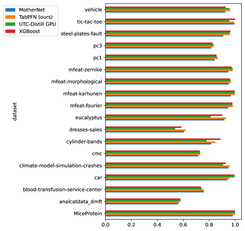
Figure 7: Subset of validation data where there is a difference of at least $0.03$ average ROC-AUC between MotherNet and MLP-distill.

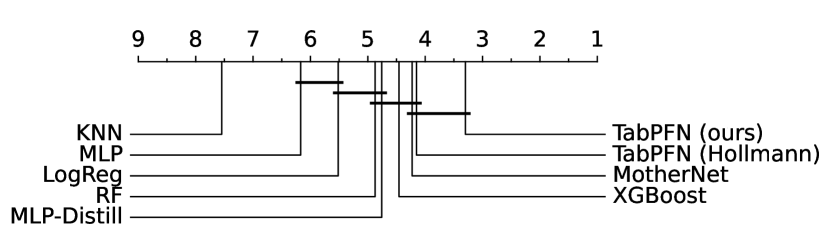
Figure 8: Critical differences diagram for the validation datasets. Baseline models are tuned for 1h per dataset.

Appendix B Validation Set Results

Experimental results for the validation set are shown in Figure 9, Figure 8. Maybe somewhat surprisingly, the ranking according to average ROC AUC and using the CD diagram are quite different; using the ranking metric, TabPFN and MotherNet win overall, while on average scores, XGBoost wins out over TabPFN, and Random Forest wins out over MotherNet. It should be noted that un-normalized averaging of ROC AUC scores is likely misleading, but the diffeerence between average and ranking points to large differences on some datasets. We confirmed this by looking at datasets with at least $0.1$ ROC AUC difference between TabPFN and XGBoost, which are shown in Figure 11. In all cases, it’s TabPFN and/or MotherNet that is drastically underperforming. It’s notable that there’s two types of datasets here. The datasets teachingAssistant and schizo have single features that are highly informative but contain strong discontinuities with respect to the target class. Both could be considered data leakage via an ID column, but in essence these point to the fact that discontinuous functions with many steps, and/or memorization of ID variables are not well captured by TabPFN and MotherNet. Two of the other datasets, parity5_plus_5 and monks-problem-1 are synthetic datasets that model higher-order boolean functions. The last dataset, GAMETES consists of categorical variables with nearly no univariate effects, so it is also likely to contain information in the higher order interactions. To confirm our intuition on these datasets, we constructed synthetic datasets to reproduce these failure cases, which are detailed in Section C.

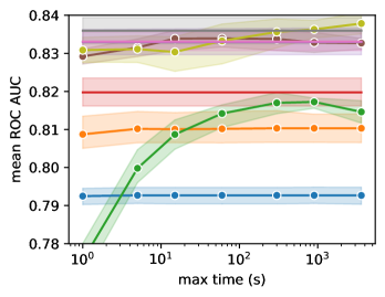
Figure 9: Comparison of TabPFN, MLP-distill and MotherNet with tuned baselines on the validation set. Left: mean normalized ROC AUC over time. Right: Mean rank over time. Predictions of transformer-based models are constant over the $x$ axis. Compare Figure 3 for test set results.

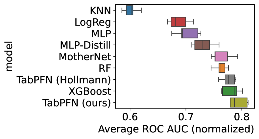
Figure 10: Comparison of normalized mean ROC AUC on validation datasets, based on tuning baselines for 1h.

Figure 11: Subset of validation data where there is a difference of at least $0.1$ average ROC-AUC between TabPFN and XGBoost.

Appendix C Failure Case Dataset Generation

Inspired by the results shown in Figure 11, we created two families of synthetic datasets. The first is a binary classification task on a single feature, that is distributed uniformly between $0$ and $1$. For each dataset that we generate, we draw $2000$ samples from the uniform distribution, and $n_{\text{steps}}-1$ cut-off points, also between $0$ and $1$. At each cut-off point we flip the class label. A resulting dataset for $n_{\text{steps}}=5$ is show in Figure 12, where we show only 100 points for illustration purposes. Note that since the split into training and test data is done using an (class-stratified) i.i.d. assumption, this dataset is trivial to learn for any tree-based or neighbors-based learner. While it is possible to learn such a dataset with a neural network, this might require tuning the architecture, and using the $MLP$ with default parameters from scikit-learn fails to learn this data.

The other family of synthetic datasets is inspired by the parity5_plus_5 dataset and is a random combination of boolean conjunctions of a certain rank. The training samples in all cases are all binary sequences of length 10, where each bit is one feature, hence the feature space is $X=\{0,1\}^{10}$. The labels for each dataset are constructed iteratively using a logical disjunction of conjunctions. In every iteration, a term is created by conjoining $r$ bits chosen at random, with each bit also randomly assigned a negation or not. Terms are continually added to the disjunction until at least one-third of the samples satisfy the formula, ensuring a relatively balanced dataset. We split the dataset randomly (but class-stratified) into training and test set. This is a relaxation of the classical parity problem; for rank $1$, the label would correspond simply to one of the input features and therefore should be easily learnable for any algorithm. For rank $10$, the dataset is an arbitrary boolean function, which is not learnable (in the sense that seeing only the training set in expectation provides no information on the test set).

For the experiments in Figure 6, we generated 20 datasets for each rank or step, and performed five-fold stratified cross-validation for each of them.

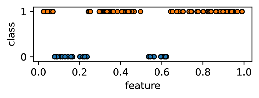
Figure 12: Example of a synthetic classification example in 1d.

Appendix D Data Leakage

We found that two of the dataset in the validation set contained data-leakage that was exploitable by tree-based models but not TabPFN or MotherNet, inspiring the analysis in Section 5. The teachingAssistant dataset (OpenML did 1115), contains a ID column that provides an ordering of rows that is strongly correlated with the target class, as shown in Figure 13. To confirm the leakage, we trained a RandomForest classifier on just the ID feature, and obtained perfect AUC in 5-fold cross-validation with just this feature. For the schizo dataset (OpenML did 466), again there is an ID column which leaks the target, but with a different mechanism. In the schizo dataset, the ID column is not unique, but instead there are 86 unique values for the 340 rows, and the class is directly determined by the ID. Again, to confirm the leakage, we trained a RandomForest classifier on just the ID feature, and obtained near-perfect AUC in 5-fold cross-validation with just this feature.

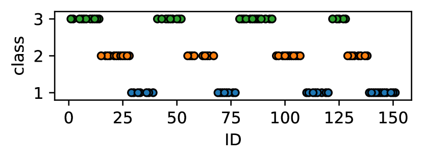
Figure 13: Correlation structure of class label and ID column in teachingAssistant dataset.

Appendix E Hyper Parameter Spaces for Baseline Methods

The hyperparameters used for the baseline models discussed in Section 4 are shown in Table 3 and were tuned with HyperOpt (Bergstra et al., 2011) following the setup of Hollmann et al. (2022).

Model	Hyperparameters
Random Forest	n_estimators: randint(20, 200), max_features: choice([None, ’sqrt’, ’log2’]),
	max_depth: randint(1, 45), min_samples_split: choice([2, 5, 10])
MLP	hidden_size: choice([16, 32, 64, 128, 256, 512]), learning_rate: loguniform($10^{-5}$, 0.01),
	n_epochs: choice([10, 100, 1000]), dropout_rate: choice([0, 0.1, 0.3]),
	n_layers: choice([1, 2, 3]), weight_decay: loguniform($10^{-5}$, 0.01)
KNN	n_neighbors: randint(1, 16)
XGBoost	learning_rate: loguniform($e^{-7}$, 1), max_depth: randint(1, 10),
	subsample: uniform(0.2, 1), colsample_bytree: uniform(0.2, 1),
	colsample_bylevel: uniform(0.2, 1), min_child_weight: loguniform($e^{-16}$, $e^{5}$),
	alpha: loguniform($e^{-16}$, $e^{2}$), lambda: loguniform($e^{-16}$, $e^{2}$),
	gamma: loguniform($e^{-16}$, $e^{2}$), n_estimators: randint(100, 4000)
Logistic Regression	penalty: choice([’l1’, ’l2’, ’none’]), max_iter: randint(50, 500),
	fit_intercept: choice([True, False]), C: loguniform($e^{-5}$, $\log(5)$)

Table 3: Hyperparameters for each model

Appendix F Validation Set

We use the validation set of (Hollmann et al., 2022), as listed in Table 4.

did	name	d	n	k
13	breast-cancer	10	286	2
25	colic	27	368	2
35	dermatology	35	366	6
40	sonar	61	208	2
41	glass	10	214	6
43	haberman	4	306	2
48	tae	6	151	3
49	heart-c	14	303	2
51	heart-h	14	294	2
53	heart-statlog	14	270	2
55	hepatitis	20	155	2
56	vote	17	435	2
59	ionosphere	35	351	2
61	iris	5	150	3
187	wine	14	178	3
329	hayes-roth	5	160	3
333	monks-problems-1	7	556	2
334	monks-problems-2	7	601	2
335	monks-problems-3	7	554	2
336	SPECT	23	267	2
337	SPECTF	45	349	2
338	grub-damage	9	155	4
377	synthetic_control	61	600	6
446	prnn_crabs	8	200	2
450	analcatdata_lawsuit	5	264	2
451	irish	6	500	2
452	analcatdata_broadwaymult	8	285	7
460	analcatdata_reviewer	8	379	4
463	backache	32	180	2
464	prnn_synth	3	250	2
466	schizo	15	340	2
470	profb	10	672	2
475	analcatdata_germangss	6	400	4
481	biomed	9	209	2
679	rmftsa_sleepdata	3	1024	4
694	diggle_table_a2	9	310	9
717	rmftsa_ladata	11	508	2
721	pwLinear	11	200	2
724	analcatdata_vineyard	4	468	2
733	machine_cpu	7	209	2
738	pharynx	11	195	2
745	auto_price	16	159	2
747	servo	5	167	2
748	analcatdata_wildcat	6	163	2
750	pm10	8	500	2
753	wisconsin	33	194	2
756	autoPrice	16	159	2
757	meta	22	528	2
764	analcatdata_apnea3	4	450	2
765	analcatdata_apnea2	4	475	2
767	analcatdata_apnea1	4	475	2
774	disclosure_x_bias	4	662	2

Table 4: Validation dataset names and properties, taken from Hollmann et al. (2022). Here did is the OpenML Dataset ID, d the number of features, n the number of instances, and k the number of classes in each dataset.

did	name	d	n	k
778	bodyfat	15	252	2
786	cleveland	14	303	2
788	triazines	61	186	2
795	disclosure_x_tampered	4	662	2
796	cpu	8	209	2
798	cholesterol	14	303	2
801	chscase_funds	3	185	2
802	pbcseq	19	1945	2
810	pbc	19	418	2
811	rmftsa_ctoarrivals	3	264	2
814	chscase_vine2	3	468	2
820	chatfield_4	13	235	2
825	boston_corrected	21	506	2
826	sensory	12	576	2
827	disclosure_x_noise	4	662	2
831	autoMpg	8	398	2
839	kdd_el_nino-small	9	782	2
840	autoHorse	26	205	2
841	stock	10	950	2
844	breastTumor	10	286	2
852	analcatdata_gsssexsurvey	10	159	2
853	boston	14	506	2
854	fishcatch	8	158	2
860	vinnie	3	380	2
880	mu284	11	284	2
886	no2	8	500	2
895	chscase_geyser1	3	222	2
900	chscase_census6	7	400	2
906	chscase_census5	8	400	2
907	chscase_census4	8	400	2
908	chscase_census3	8	400	2
909	chscase_census2	8	400	2
915	plasma_retinol	14	315	2
925	visualizing_galaxy	5	323	2
930	colleges_usnews	34	1302	2
931	disclosure_z	4	662	2
934	socmob	6	1156	2
939	chscase_whale	9	228	2
940	water-treatment	37	527	2
941	lowbwt	10	189	2
949	arsenic-female-bladder	5	559	2
966	analcatdata_halloffame	17	1340	2
968	analcatdata_birthday	4	365	2
984	analcatdata_draft	5	366	2
987	collins	23	500	2
996	prnn_fglass	10	214	2
1048	jEdit_4.2_4.3	9	369	2
1054	mc2	40	161	2
1071	mw1	38	403	2
1073	jEdit_4.0_4.2	9	274	2
1100	PopularKids	11	478	3
1115	teachingAssistant	7	151	3
1412	lungcancer_GSE31210	24	226	2
1442	MegaWatt1	38	253	2

Table 5: Validation datasets, continued

did	name	d	n	k
1443	PizzaCutter1	38	661	2
1444	PizzaCutter3	38	1043	2
1446	CostaMadre1	38	296	2
1447	CastMetal1	38	327	2
1448	KnuggetChase3	40	194	2
1451	PieChart1	38	705	2
1453	PieChart3	38	1077	2
1488	parkinsons	23	195	2
1490	planning-relax	13	182	2
1495	qualitative-bankruptcy	7	250	2
1498	sa-heart	10	462	2
1499	seeds	8	210	3
1506	thoracic-surgery	17	470	2
1508	user-knowledge	6	403	5
1511	wholesale-customers	9	440	2
1512	heart-long-beach	14	200	5
1520	robot-failures-lp5	91	164	5
1523	vertebra-column	7	310	3
4153	Smartphone-Based_Recognition…	68	180	6
23499	breast-cancer-dropped-…	10	277	2
40496	LED-display-domain-7digit	8	500	10
40646	GAMETES_Epistasis_2-Way…	21	1600	2
40663	calendarDOW	33	399	5
40669	corral	7	160	2
40680	mofn-3-7-10	11	1324	2
40682	thyroid-new	6	215	3
40686	solar-flare	13	315	5
40690	threeOf9	10	512	2
40693	xd6	10	973	2
40705	tokyo1	45	959	2
40706	parity5_plus_5	11	1124	2
40710	cleve	14	303	2
40711	cleveland-nominal	8	303	5
40981	Australian	15	690	2
41430	DiabeticMellitus	98	281	2
41538	conference_attendance	7	246	2
41919	CPMP-2015-runtime-classification	23	527	4
41976	TuningSVMs	81	156	2
42172	regime_alimentaire	20	202	2
42261	iris-example	5	150	3
42544	Touch2	11	265	8
42585	penguins	7	344	3
42638	titanic	8	891	2

Table 6: Validation dataset, continued

References

- Abdulrahman et al. (2018) Abdulrahman, S. M., Brazdil, P., van Rijn, J. N., and Vanschoren, J. Speeding up algorithm selection using average ranking and active testing by introducing runtime. Machine learning, 107:79–108, 2018.
- Andrychowicz et al. (2016) Andrychowicz, M., Denil, M., Gomez, S., Hoffman, M. W., Pfau, D., Schaul, T., Shillingford, B., and De Freitas, N. Learning to learn by gradient descent by gradient descent. Advances in neural information processing systems, 29, 2016.
- Bergstra et al. (2011) Bergstra, J., Bardenet, R., Bengio, Y., and Kégl, B. Algorithms for hyper-parameter optimization. Advances in Neural Information Processing Systems, 24, 2011.
- Bertinetto et al. (2016) Bertinetto, L., Henriques, J. F., Valmadre, J., Torr, P., and Vedaldi, A. Learning feed-forward one-shot learners. Advances in neural information processing systems, 29, 2016.
- Bischl et al. (2017) Bischl, B., Casalicchio, G., Feurer, M., Gijsbers, P., Hutter, F., Lang, M., Mantovani, R. G., van Rijn, J. N., and Vanschoren, J. Openml benchmarking suites. arXiv preprint arXiv:1708.03731, 2017.
- Brazdil et al. (2003) Brazdil, P. B., Soares, C., and Da Costa, J. P. Ranking learning algorithms: Using ibl and meta-learning on accuracy and time results. Machine Learning, 50:251–277, 2003.
- Breiman (2001) Breiman, L. Random forests. Machine learning, 45:5–32, 2001.
- Brown et al. (2020) Brown, T., Mann, B., Ryder, N., Subbiah, M., Kaplan, J. D., Dhariwal, P., Neelakantan, A., Shyam, P., Sastry, G., Askell, A., et al. Language models are few-shot learners. Advances in neural information processing systems, 33:1877–1901, 2020.
- Chen & Guestrin (2016) Chen, T. and Guestrin, C. Xgboost: A scalable tree boosting system. In Proceedings of the 22nd acm sigkdd international conference on knowledge discovery and data mining, pp. 785–794, 2016.
- Chui et al. (2018) Chui, M., Manyika, J., Miremadi, M., Henke, N., Chung, R., Nel, P., and Malhotra, S. Notes from the ai frontier: Insights from hundreds of use cases. McKinsey Global Institute, 2, 2018.
- Demšar (2006) Demšar, J. Statistical comparisons of classifiers over multiple data sets. The Journal of Machine learning research, 7:1–30, 2006.
- Finn et al. (2017) Finn, C., Abbeel, P., and Levine, S. Model-agnostic meta-learning for fast adaptation of deep networks. In International conference on machine learning, pp. 1126–1135. PMLR, 2017.
- Friedman (2001) Friedman, J. H. Greedy function approximation: a gradient boosting machine. Annals of statistics, pp. 1189–1232, 2001.
- Ha et al. (2017) Ha, D., Dai, A., and Le, Q. V. Hypernetworks. 2017. URL https://openreview.net/pdf?id=rkpACe1lx.
- Hinton et al. (2015) Hinton, G., Vinyals, O., and Dean, J. Distilling the knowledge in a neural network. arXiv preprint arXiv:1503.02531, 2015.
- Hollmann et al. (2022) Hollmann, N., Müller, S., Eggensperger, K., and Hutter, F. TabPFN: A transformer that solves small tabular classification problems in a second. In NeurIPS 2022 First Table Representation Workshop, 2022. URL https://openreview.net/forum?id=eu9fVjVasr4.
- Hutter et al. (2019) Hutter, F., Kotthoff, L., and Vanschoren, J. Automated machine learning: methods, systems, challenges. Springer Nature, 2019.
- Iida et al. (2021) Iida, H., Thai, D., Manjunatha, V., and Iyyer, M. Tabbie: Pretrained representations of tabular data. arXiv preprint arXiv:2105.02584, 2021.
- Ke et al. (2017) Ke, G., Meng, Q., Finley, T., Wang, T., Chen, W., Ma, W., Ye, Q., and Liu, T.-Y. Lightgbm: A highly efficient gradient boosting decision tree. Advances in neural information processing systems, 30, 2017.
- Li & Liang (2021) Li, X. L. and Liang, P. Prefix-tuning: Optimizing continuous prompts for generation. arXiv preprint arXiv:2101.00190, 2021.
- Loshchilov & Hutter (2016) Loshchilov, I. and Hutter, F. Sgdr: Stochastic gradient descent with warm restarts. arXiv preprint arXiv:1608.03983, 2016.
- Müller et al. (2021) Müller, S., Hollmann, N., Arango, S. P., Grabocka, J., and Hutter, F. Transformers can do bayesian inference. arXiv preprint arXiv:2112.10510, 2021.
- OpenAI (2023) OpenAI. Gpt-4 technical report, 2023.
- Pedregosa et al. (2011) Pedregosa, F., Varoquaux, G., Gramfort, A., Michel, V., Thirion, B., Grisel, O., Blondel, M., Prettenhofer, P., Weiss, R., Dubourg, V., et al. Scikit-learn: Machine learning in python. the Journal of machine Learning research, 12:2825–2830, 2011.
- Ravi & Larochelle (2016) Ravi, S. and Larochelle, H. Optimization as a model for few-shot learning. In International conference on learning representations, 2016.
- Rivolli et al. (2018) Rivolli, A., Garcia, L. P. F., Soares, C., Vanschoren, J., and de Carvalho, A. C. P. L. F. Towards reproducible empirical research in meta-learning. CoRR, abs/1808.10406, 2018. URL http://arxiv.org/abs/1808.10406.
- Schmidhuber (1992) Schmidhuber, J. Learning to control fast-weight memories: An alternative to dynamic recurrent networks. Neural Computation, 4(1):131–139, 1992.
- Tancik et al. (2020) Tancik, M., Srinivasan, P., Mildenhall, B., Fridovich-Keil, S., Raghavan, N., Singhal, U., Ramamoorthi, R., Barron, J., and Ng, R. Fourier features let networks learn high frequency functions in low dimensional domains. Advances in Neural Information Processing Systems, 33:7537–7547, 2020.
- Tay et al. (2022) Tay, Y., Dehghani, M., Bahri, D., and Metzler, D. Efficient transformers: A survey. ACM Computing Surveys, 55(6):1–28, 2022.
- Thrun & Pratt (1998) Thrun, S. and Pratt, L. Learning to learn: Introduction and overview. In Learning to learn, pp. 3–17. Springer, 1998.
- Touvron et al. (2023) Touvron, H., Lavril, T., Izacard, G., Martinet, X., Lachaux, M.-A., Lacroix, T., Rozière, B., Goyal, N., Hambro, E., Azhar, F., et al. Llama: Open and efficient foundation language models. arXiv preprint arXiv:2302.13971, 2023.
- Vanschoren (2018) Vanschoren, J. Meta-learning: A survey. arXiv preprint arXiv:1810.03548, 2018.
- Vaswani et al. (2017) Vaswani, A., Shazeer, N., Parmar, N., Uszkoreit, J., Jones, L., Gomez, A. N., Kaiser, Ł., and Polosukhin, I. Attention is all you need. Advances in neural information processing systems, 30, 2017.
- Wistuba et al. (2015) Wistuba, M., Schilling, N., and Schmidt-Thieme, L. Sequential model-free hyperparameter tuning. In 2015 IEEE international conference on data mining, pp. 1033–1038. IEEE, 2015.
- Yeo & Johnson (2000) Yeo, I.-K. and Johnson, R. A. A new family of power transformations to improve normality or symmetry. Biometrika, 87(4):954–959, 2000.
- Yin et al. (2020) Yin, P., Neubig, G., Yih, W.-t., and Riedel, S. Tabert: Pretraining for joint understanding of textual and tabular data. arXiv preprint arXiv:2005.08314, 2020.
- Zhao et al. (2020) Zhao, D., Kobayashi, S., Sacramento, J., and von Oswald, J. Meta-learning via hypernetworks. In 4th Workshop on Meta-Learning at NeurIPS 2020 (MetaLearn 2020). NeurIPS, 2020.
- Zintgraf et al. (2019) Zintgraf, L., Shiarli, K., Kurin, V., Hofmann, K., and Whiteson, S. Fast context adaptation via meta-learning. In International Conference on Machine Learning, pp. 7693–7702. PMLR, 2019.