Coexistence of Satellite-borne Passive Radiometry and Terrestrial NextG Wireless Networks in the 1400-1427 MHz Restricted L-Band

Abstract

The rapid growth of wireless technologies has fostered research on spectrum coexistence worldwide. One idea that is gaining attention is using frequency bands solely devoted to passive applications, such as passive remote sensing. One such option is the 27 MHz L-band spectrum from 1.400 GHz to 1.427 GHz. Active wireless transmissions are prohibited in this passive band due to radio regulations aimed at preventing Radio Frequency Interference (RFI) on highly sensitive passive radiometry instruments. The Soil Moisture Active Passive (SMAP) satellite, launched by the National Aeronautics and Space Administration (NASA), is a recent space-based remote sensing mission that passively scans the Earth’s electromagnetic emissions in this 27 MHz band to assess soil moisture on a global scale periodically. This paper evaluates using the restricted L-band for active terrestrial wireless communications through two means. First, we investigate an opportunistic temporal use of this passive band within a terrestrial wireless network, such as a cluster of cells, during periods when there is no Line of Sight (LoS) between SMAP and the terrestrial network. Second, leveraging stochastic geometry, we assess the feasibility of using this passive band within a large-scale network in LoS of SMAP while ensuring that the error induced on SMAP’s measurements due to RFI is below a given threshold. The methodology established here, although based on SMAP’s specifications, is adaptable for utilization with various passive sensing satellites regardless of their orbits or operating frequencies.

I Introduction

Besides those at absolute zero Kelvin, all objects emit electromagnetic radiation due to their body temperature (natural thermal emissions) [1]. In Remote Sensing (RS), thermal radiations from land, oceans, atmosphere, and vegetation are extremely useful in climate and geology sciences, as they can provide us with invaluable information about soil moisture (SM), sea surface salinity (SSS), and other climatological and geological variables. As climate change escalates, this information becomes even more critical in many applications, including weather, flood, and drought forecasting, as well as agricultural productivity, carbon cycle, and hydrological modeling [2].

Although thermal emissions from objects exist on a wide range of frequencies, some frequency bands are more favorable for different RS applications. For example, L-band spectrum ( 1–2 GHz) is optimal for sensing SM because of its relatively high sensitivity to the moisture content in deeper soil, its semi-transparency to vegetation covering the soil, and lower attenuation from the atmosphere[3]. Such favorable properties have inspired the allocation of several portions of the frequency spectrum for various passive RS applications, including the L-band (1.4 GHz), C-band (6 GHz), X-band (10 GHz), and mm-wave frequencies ($>$30 GHz) [4]. For some passive bands, Federal Communications Commission (FCC) radio regulations disallow in-band active wireless transmissions and out-of-band spectral leakage from adjacent bands [4].

In parallel, the proliferation of Next-G networks demands enhanced, reliable, and ubiquitous connectivity to support various applications with faster speeds, reduced latency, and massive numbers of connected devices. This will require improving utilization of the frequency spectrum [5] and will further exacerbate the so-called spectrum crunch [6]. With the limited availability of radio frequency spectrum, network operators and regulatory bodies face the task of efficiently allocating and managing this valuable resource.

One solution gaining attention is the use of passive bands for active wireless communications [7]. However, this increases the risk of active wireless devices inducing radio frequency interference (RFI) on passive sensing instruments. Since these instruments are designed to measure faint natural emissions, even weak RFI can lead to erroneous measurements. Worse still, strong RFI can potentially saturate the passive radiometry electrical equipment, rendering it inoperable. The conflict between active and passive users of the spectrum calls for research on active-passive coexistence in spectrally adjacent bands or in co-channel (i.e., in the same frequency band). An indispensable step in this course is evaluating the amount of RFI that active Next-G devices induce on passive sensing instruments, which can then help us determine the degree to which Next-G devices can utilize passive bands without compromising the incumbent passive sensing instruments’ operations and the science that relies on their measurements.

Among various passive sensing methodologies, spaceborne passive sensing has gained significant importance due to the comprehensive coverage it can provide in a short time [2]. A notable benefit is the ability to employ a single sensor globally and for an extended duration. This allows for more accurate monitoring of changes in the observed natural phenomena across different geographical areas and time spans. It also overcomes the limitations of using multiple instruments with different calibrations, ensuring greater precision in data tracking.

One frequency band commonly used for space-borne passive radiometry missions is the 27 MHz narrow-band of the L-band portion of the frequency spectrum from 1.400 GHz to 1.427 GHz, i.e., the restricted L-band, which is exclusively devoted to passive radiometry for Earth Exploration Satellites, Radio Astronomy, and Space Research, according to Federal Communications Commission (FCC) radio regulations [4]. The contemporary L-band passive remote space missions can be traced back to the launch of the European Space Agency’s (ESA) Soil Moisture and Ocean Salinity (SMOS) Satellite in 2009 [8], followed by the National Aeronautics and Space Administration’s (NASA) Aquarius satellite in 2011 [9]. Launched in 2015, NASA’s Soil Moisture Active Passive (SMAP) satellite is the latest space-borne RS mission operating in this band [10]. SMAP provides data on soil moisture through point-wise scanning of soil’s passive electromagnetic thermal radiations with high resolution Earth footprints every 2 to 3 days.

In this paper, we investigate how a large-scale terrestrial NextG network can share the spectrum with NASA’s SMAP in the restricted L-band. Given that SMAP is a Low Earth Orbit (LEO) satellite [11], it does not maintain fixed position relative to the Earth at all times. Consequently, at each time, the Earth’s surface is partitioned into two distinct regions: one region where there is Line of Sight (LoS) between SMAP and the NextG network (and hence SMAP is exposed to the network) and another region where there is no LoS (and hence SMAP is not exposed to the network).

• We propose opportunistic temporal use of the restricted L-band when SMAP is not exposed to a NextG network site. This strategy will prevent SMAP’s direct exposure to RFI from the network site. For this purpose, for NextG network sites located at different Earth locations, we examine the ratio of time SMAP is not exposed to them (exposure-free time ratio) during its three-day global coverage time.

• Based on simulations using SMAP’s orbital characteristics, we show that the exposure-free time ratio is predominantly affected by a NextG network site’s Earth latitude. Based on simulations, we show the minimum exposure-free time ratio is $86.43\%$ for equatorial regions while its maximum value is $96.82\%$ for polar regions.

• Regarding regions of Earth in LoS with SMAP, we employ stochastic geometry to examine the viability of having a large-scale NextG network active in the restricted L-band. To the best of our knowledge, this is the first work that uses stochastic geometry to assess the aggregate RFI from a NextG network on a passive remote sensing satellite. To model the aggregate RFI on SMAP, we use a Thomas Poisson Cluster Process to model the NextG network as a constellation of clusters, where each cluster represents a dense urban area with multiple active cellular base stations (BSs).

• Employing the acquired stochastic geometry model, we establish a balance between the NextG network parameters including the number of active clusters and cellular base stations, and the degree of disruption inflicted upon SMAP’s measurement accuracy.

While the methodology established here derives from SMAP’s specifications, it is adaptable to other passive sensing satellites operating in different frequency bands and orbits.

The rest of the paper is organized as follows. In Section II, we discuss related work on spectrum coexistence between terrestrial and satellite communication networks. In Section III, we present the orbital characteristics of the SMAP satellite and investigate the opportunistic temporal transmissions within a terrestrial network. In Section III, we analyze the spectrum coexistence of SMAP with a global-scale terrestrial wireless network under LoS conditions. In Section V, we present the simulation results. We conclude the paper in Section VI.

II Related Work

In [12], we investigated opportunistic temporal spectrum coexistence between a large-scale terrestrial network and SMAP during periods when there is no LoS between SMAP and the terrestrial network. In contrast, in this paper, we use stochastic geometry to model the impact of the aggregate RFI induced on a remote sensing satellite such as SMAP by a large-scale terrestrial cellular network in LoS with the satellite. To the best of our knowledge, this is the first work to use stochastic geometry in an Earth-space active-passive scenario between a terrestrial active wireless communication network and a passive sensing space object. In the absence of comparable research, we first briefly introduce the existing research concerning active-passive spectrum sharing, i.e., the coexistence of active wireless communications and passive sensing technologies, e.g., passive remote sensing and radio astronomy. Another category of research that has inspired us on the geometry analysis for Earth-space RFI modeling is the active-active spectrum coexistence in scenarios containing both active terrestrial and space components. This scope of research will be also briefly reviewed in this section. Additionally, another established realm of research, which is partially addressed within this study, focuses on the identification and alleviation of RFI in passive remote sensing technologies, rather than tackling the coexistence of active-passive technologies in the spectrum.

Polese et al. [7] investigate the allocation of large chunks of continuous bandwidths for future 6G wireless networks operating above 100 GHz, where multiple narrow passive sensing sub-bands scatter over the frequency spectrum, precluding the allocation of large continuous bandwidth chunks. In their work, they consider a wireless link between two terrestrial base stations interfering with an Earth Exploration Satellite Service (EESS) satellite. Using International Telecommunication Union (ITU) recommendations, they develop a path loss model between the interfering base stations and the EESS satellite. The main distinction from our work is that they do not take into account the coexistence of a large network within the LoS of a passive sensing satellite

Zheleva et al. [13] propose the idea of Radio Dynamic Zones (RDZ) as experimental testbeds for spectrum research. These testbeds enable the study of the coexistence of different technologies used by three major frequency spectrum stakeholders: consumer broadband, microwave remote sensing, and radio astronomy. The RDZs are regional-scale geographic areas of $10$s to $100$s of square kilometers, where these diverse stakeholders can conduct research on spectrum coexistence.

In [14], authors investigate spectrum coexistence between Cellular Wireless Communications (CWC) and terrestrial Radio Astronomy Systems (RAS). They propose a geographical Shared Spectrum Access Zone (SSAZ) around a RAS site in which there is a three-phase spectrum access for the surrounding cellular network based on the distance to the RAS site. Also, the network outside the SSAZ has full spectrum access. They considered both deterministic hexagonal CWC cells and a 2-dimensional Poisson Point Process to model the cellular network surrounding a RAS site.

In the following, we provide a brief introduction to related work on the active-active RFI problem in scenarios involving both terrestrial and space components. In [15], Jung et al. investigate downlink LEO satellite communication systems. In their model, they assume a constellation of LEO satellites is distributed around the Earth according to a Binomial Point Process (BPP) at a certain altitude. The primary focus of their analysis is on the communication link from an individual satellite to its corresponding Earth base station. Within this context, they evaluate the likelihood of communication disruptions caused by RFI stemming from the sidelobe emissions of neighboring satellites.

Han et al. [16] investigate the adjacent channel coexistence of Time Division Long Term Evolution (TD-LTE) with the Compass navigation satellite system (COMPASS) in the same geographical area. Using stochastic geometry, they calculate the outage probability of COMPASS service on Earth due to the interference from TD-LTE cells in a region. Moreover, they develop a resource scheduling approach called Maximum Adjacent Channel Interference Ratio (Max-ACIR) that lessens interference induced on the COMPASS downlink from the TD-LTE uplink.

Zhang et al. [17] calculate RFI on a communication link between a geostationary (GEO) satellite and its associated ground base station caused by lower orbit satellites and terrestrial 5G networks. In their model, they assume the operational frequency for the GEO is $17.7-19.7$ GHz and $27.5-29.5$ GHz devoted to Fixed Satellite Services (FSS), Fixed Services (FS), and Mobile Services (MS). They calculate the minimum distance $R$ that the non-geostationary and 5G base stations must be away from the GEO ground station to at least preserve the minimum required bit rate between the GEO base station and its associated satellite.

Latachi et al. [18] determine the requirements for establishing a reliable connection between a ground base station and a CubeSat satellite. They first calculate the frequency shift due to the CubeSat’s velocity using a simplified 2-dimensional model of the earth and the satellite’s orbit. Next, they develop a simplified model for the attenuation caused by distance and atmospheric effects for frequencies below 3 GHz; they calculate the impact of the thermal noise radiated from the transmitter (located on Earth) to the satellite’s receiver; and, using Friis law, they calculate the effect of noise on cascaded electrical components and amplifiers in the receiver.

Del Re et al. [19] investigate a cognitive radio approach for a meshed OFDM-based secondary terrestrial wireless service to coexist with a primary terrestrial and satellite Digital Video Broadcasting Satellite To Handheld (DVB-SH) system in the L-band (0.39-1.55 GHz). Because the secondary system is cognitive, its flexibility over power allocation, frequency, and modulation schemes is exploited to maximize its bit rate with a maximum tolerable Bit Error Rate (BER) while maintaining the primary systems’ BER below a specified target.

Khawar et al. [20] investigate the deployment of small terrestrial cells (both indoor and outdoor) in the satellite frequencies adjacent to conventional and extended C-band Fixed Satellite Services (FSS) receiving Earth stations. Their work shows that out-of-band emissions from small cells can cause Low Noise Amplifier (LNA) saturation for FSS receivers; therefore, exclusion zones are required to protect FSS systems. They also show that exclusion zones should be relatively larger when small cells are deployed outdoors rather than indoors.

Janhunen et al. [21] explore the impact of RFI from a terrestrial LTE network on the uplink of a satellite-extended LTE network. In their study, the LTE cellular network is situated in a densely populated urban area, while the satellite-extended LTE network covers a nearby rural region. In the satellite-extended LTE network, a User Equipment (UE) device directly connects to a satellite’s uplink, and the uplink transmissions from UEs and their respective base stations in the neighboring terrestrial LTE network can introduce interference. Using a simulator based on Single-Carrier Frequency-Division Multiple Access (SC-FDMA) LTE technology, the authors demonstrate that despite the long satellite communication link, strict power limitations at the UE end, and interference from adjacent terrestrial networks, the satellite link can operate on the same frequency range as the terrestrial network.

It is worth mentioning another category of articles that focuses on diagnosing RFI and mitigating its effects on passive sensing satellites. These studies primarily examine the impact of RFI and do not delve into the concept of spectrum coexistence. In the following discussion, we explore two recent articles that specifically address the issue of RFI on SMAP.

In [22], Mohammed et al. leverage Deep Learning (DL) for RFI detection in SMAP. Using a supervised learning approach, they feed the spectrograms produced by SMAP as inputs to Convolutional Neural Networks (CNNs) that classify the spectrograms into “RFI” and “No RFI” groups. To enable training of the classifiers using a small dataset from SMAP, they replace and retrain the last few layers of pre-trained CNN models (ResNet-101, AlexNet, and GoogleNet) with spectrograms from SMAP. In their dataset, they use spectrograms with different RFI levels, including low ($5$ - $10$ K), intermediate ($10$ - $100$ K), and high ($>100$ K) levels from across the globe. The RFI has different types, including pulsed, Continuous Wave (CW), and wideband. They provide RFI-free spectrograms from RFI-free parts of the world with RFI levels below 2 K.

The current interference mitigation techniques used for the SMAP passive radiometer involve detecting and flagging contaminated samples and then discarding them, which leads to the loss of data, especially in severe cases of RFI. To prevent the loss of information, the authors in [23] proposed a novel interference mitigation method based on an autoencoder for the SMAP passive radiometer. This method focuses on reconstructing clean readings from the contaminated samples rather than discarding them. This innovative idea not only preserves valuable information but also paves the way for new ways of coexistence between terrestrial users and space-borne passive radiometers, as it makes the radiometers more robust against RFI.

In comparison to existing research on the coexistence of active-passive spectrums, which primarily involves terrestrial passive sensing elements like terrestrial radio astronomy sites and active terrestrial wireless networks, We delve into the RFI issue caused by an active terrestrial network affecting a passive sensing object positioned in space. This work also distinctly deviates from studies addressing RFI concerns in active-active Earth-satellite communication systems.

III Preliminaries & Temporal Spectrum Coexistence

While temporal spectrum coexistence between different active wireless systems, such as wireless communication networks and radars [24, 25], has been extensively studied, investigation of it between active and passive systems has been relatively limited. One objective of our research is to assess temporal spectrum coexistence between a terrestrial NextG wireless network and SMAP, by allowing the NextG network to transmit when SMAP is absent from its sky. To this end, we investigate the importance of the NextG network’s latitude on Earth to analyze the exposure time and exposure-free time ratios during SMAP’s global coverage period.

III-A SMAP’s Orbit & Rotational Movement

SMAP follows a near-polar Sun-synchronous orbit (SSO), commonly referred to as the “6 am/6 pm orbit,” deviating from the equator by $98.12\degree$. In this orbit, SMAP passes over each point on Earth at the same local mean solar time, as shown in Figure 1(a), and circles the Earth every 98 minutes at an altitude of 685 km, as illustrated in Figure 1(b) [12, 26].

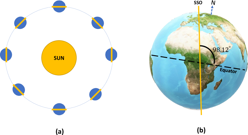
Figure 1: (a) Near polar Sun-synchronous orbit (SSO). (b) Near-polar SSO with respect to Earth’s axis and the equator.

SMAP’s radiometer has a 6-meter-diameter golden mesh reflector with a horn that has a beam-width of $2.4\degree$, as depicted in Figure 2. At an incidence angle of approximately $40\degree$, the reflector creates a footprint of $40\times 40$ km² on the Earth’s surface, capturing thermal radiations from the soil in the $1400$ to $1427$ MHz restricted L-band. Operating at a speed of $14.5$ revolutions per minute (RPM), the horn and reflector cover a swath that spans $1000$ km along SMAP’s nadir track. Full Earth coverage happens in $2$ to $3$ days, while a complete orbit where SMAP returns to its starting point takes $8$ days [12, 26].

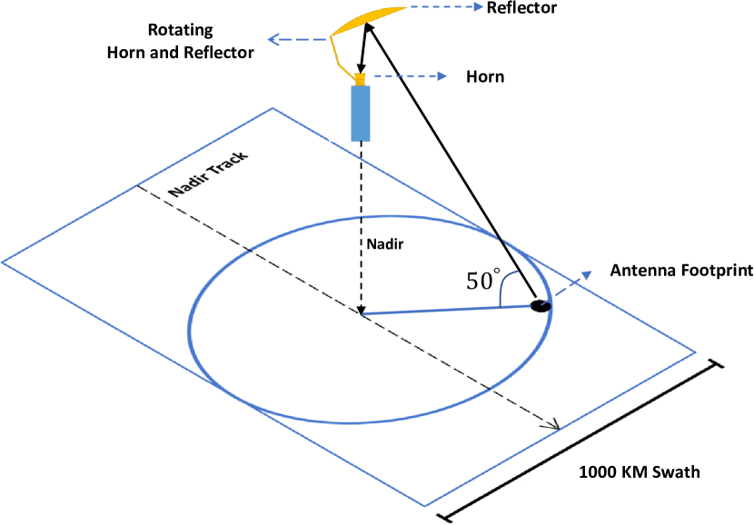
Figure 2: Horn and reflector rotation, beam footprint of the reflector, and SMAP’s nadir track.

III-B Temporal Spectrum Coexistence

For each NextG network site around the world, time can be divided into two alternating phases: periods when the cellular site has LoS to the satellite (equivalently, SMAP is visible in the cellular site’s sky), and intervals when it does not. When the network is not visible to the satellite, we propose that it opportunistically leverages the restricted L-band for wireless transmissions.

The key point to consider is that exposure to SMAP for cellular sites situated at different locations on Earth varies based on SMAP’s orbital attributes. For example, during a particular time window, some regions might experience more extended periods of exposure to SMAP compared to others. Consequently, we investigate the impact of the cellular site’s latitude and longitude on its exposure to SMAP. For each geographical location, we assess two specific metrics. First, the exposure-free time ratio, which represents the proportion of time when the cellular site has no exposure to SMAP during its three-day global coverage period. Second, the number of exposure events, indicating how many times SMAP becomes visible in the cellular site’s sky during its three-day global coverage period. Our simulations reveal that the primary determining factor for these metrics is the cellular site’s latitude, rather than its longitude. In Section V-A, we comprehensively evaluate these two metrics for cellular sites located at various Earth latitudes.

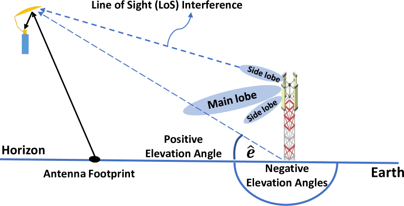
Figure 3: SMAP satellite and an interfering NextG BS. A positive elevation angle means direct LoS between SMAP and the BS, while a negative elevation angle means SMAP is below the horizon.

To determine whether a cellular site is exposed to SMAP, we rely on the concept of the elevation angle. This angle represents the incline between the horizon, the cellular site, and the SMAP satellite, as illustrated in Figure 3. In this diagram, a positive elevation angle signifies exposure to the satellite, while a negative angle indicates that the satellite is below the horizon as viewed from the cellular site, consequently, there is no LoS from the cellular site to SMAP. As a result, cellular sites situated in locations with negative elevation angles can opportunistically transmit within the restricted L-band until the next appearance of SMAP in their sky. It is important to acknowledge that a positive elevation angle does not necessarily guarantee direct exposure to SMAP, as natural obstacles like buildings, mountains, or vegetation could obstruct the view. However, for the sake of simplicity, these scenarios are not addressed in this paper. Instead, considering this simplifying assumptions, we provide a worst-case analysis in terms of exposure times. By monitoring the elevation angle using SMAP’s orbital specifications and auxiliary synchronization data, cellular sites across the globe can opportunistically use the restricted L-band without direct LoS exposure to a passive remote sensing satellite like SMAP.

IV LoS Spectrum Coexistence

In contrast to the previous section, we now shift our focus to examining the coexistence of a large-scale terrestrial NextG network in LoS of SMAP. Specifically, we explore the conditions that must be met to ensure that the NextG network does not exceed the acceptable RFI limit imposed on SMAP’s measurements. By investigating these factors, we aim to identify the requirements for maintaining a harmonious coexistence between a NextG network and SMAP while preserving the integrity and accuracy of SMAP’s data. Although deterministic models based on system-level simulations are precise for small-scale networks, they can be infeasible and error-prone for large-scale networks [27]. Therefore, we resort to mathematical tools, including stochastic geometry [28, 29, 30, 27], to model the aggregate RFI on SMAP induced by a large-scale terrestrial NextG wireless network. However, before we can model the aggregate RFI, we need to model various components of the problem, including the Earth-space path loss (comprising atmospheric losses, BS antenna gains, and SMAP’s radiometer antenna gain), the impact of RFI on the brightness temperature measured by SMAP, and the geometry of the system. Subsequently, we establish the network parameters by utilizing stochastic geometry models.

IV-A Earth-Space Path Loss Model

In this section, we model the path loss from a NextG BS to SMAP. For this purpose, we consider the following path loss equation based on the ITU-R model [31]:

$$PL=10\alpha\log_{10}(x)+20\log_{10}(f)\\ +32.45+A_{l}+G_{BS}+G_{SMAP}\quad\text{dB},$$ (1)

where $x$ denotes the distance between the NextG BS and the satellite in meters; $f$ denotes the carrier frequency of the BS in GHz; and $A_{l}$, $G_{BS}$, and $G_{SMAP}$ denote the atmospheric path loss, BS antenna gain, and SMAP’s radiometer antenna gain, respectively.

Equation (1) incorporates the parameter $\alpha$, which represents the path loss exponent. In the case of free-space path loss (FPSL), this exponent has a value of two [32]. Nevertheless, it is important to note that the free space path loss model provides an average estimation and is significantly simplified compared to real-world scenarios where numerous interfering effects exist [31]. According to [31], $\alpha$ can have values up to $6$ for outdoor transmitters and can be greater for indoor antennas based on the number of penetrated floors. Also, in [33], research on the path loss exponent for ground-to-air communication in airports shows path loss exponents of up to $4$ for LoS wireless links, and up to $5.4$ for Non-LoS links in the Very High Frequency (VHF) band.

Rewriting (1) in linear form, we obtain

$$PL=Ax^{-\alpha},$$ (2)

where

$$A=10^{-(\frac{A_{l}}{10}+\frac{G_{BS}}{10}+\frac{G_{SMAP}}{10}+3.245)}f^{-2}.$$ (3)

Accordingly, the interference power received at SMAP from a BS can be expressed compactly as:

$$P_{BS}=P_{tx}Ax^{-\alpha},$$ (4)

where $P_{tx}$ is the transmission power of the BS. In subsections IV-B, IV-C, and IV-D, we further examine the other path loss elements present in (1).

IV-B Atmospheric Path Loss

As in (1), attenuation due to the atmospheric effects ($A_{l}$) has to be taken into consideration for air-to-space transmissions. According to [34], we can identify the following causes for Earth-to-space atmospheric electromagnetic attenuation: attenuation due to polarization mismatch, attenuation due to atmospheric gases, beam spreading loss, and scintillation.

• Depolarization attenuation is due to either Faraday rotation or Hydrometer scattering that causes the rotation of the polarization of the beam ray [34]. As we will detail in Section IV-D, SMAP is equipped with a dual-polarized antenna, enabling it to fully capture electromagnetic beam rays regardless of their polarization rotation. Therefore, we ignore depolarization attenuation.

• Attenuation due to the absorption of atmospheric gases [32, 35] happens mostly due to the existence of oxygen and water vapor in Earth’s Atmosphere and is a complicated function of frequency. Since water vapor is the dominant cause of attenuation, temporal and spatial variations of water vapor in the atmosphere can cause massive variations in path loss [36]. According to [34], gaseous path loss is mostly negligible for frequencies below $2$ GHz.

• Loss due to beam spreading is caused by the refractive effect of the atmosphere and is negligible for elevation angles above $5\degree$ and can be ignored for frequencies below 10 GHz [34].

• Scintillation is caused by ionospheric scintillation [37] or tropospheric scintillation [37], which causes rapid signal-level fluctuations in time and over short distances. According to [34], ionospheric scintillation is negligible for frequencies below 10 GHz, and tropospheric scintillation is also insignificant for frequencies below 4 GHz.

In Section V-B, we investigate atmospheric path loss, and show that it has a negligible effect in the restricted L-band.

IV-C Base Station Antenna Model

In the context of (1), it is crucial to consider the BS’s antenna gain, denoted as $G_{BS}$, in the Earth-to-space path loss model. Cellular antennas are typically designed with a vertical downtilt angle, achieved by either mechanical downtilt (MDT) or electrical downtilt (EDT), which varies from a few degrees to several tens of degrees [38, 39]. This down-tilt angle directs the main lobe gain of the antenna toward the ground, ensuring efficient coverage of the intended service area while reducing interference with neighboring cells.

As observable in Fig. 4, the main lobe of a cellular BS with height $a$ and beam-width $BM$ will not hit SMAP (even at the horizon) if the following inequality holds:

$$\cos\left(DT-\frac{BM}{2}\right){\color[rgb]{0,0,0}{<}}\frac{r}{r+a}.$$ (5)

Rearranging (5), we conclude that the down-tilt angle ($DT$) must satisfy the following inequality so that the main lobe does not hit SMAP within its beamwidth:

$$DT>\arccos\left(\frac{r}{r+a}\right)+\frac{BM}{2}.$$ (6)

In (6), $r$ is the Earth’s radius, which is greater than $6000$ km, while the height of a cellular tower $a$ is in the range of tens of meters, therefore in (6) $\arccos\left(\frac{r}{r+a}\right)\approx 0{\degree}$, and for avoiding main lobe interference the following inequality suffices:

$$DT>\frac{BM}{2}.$$ (7)

[40, Eqs. (7) and (8)] certify that (7) holds. Consequently, we expect that the primary source of interference at SMAP would arise from the BS antenna’s side lobes rather than its main lobe, as shown in Fig. 3. However, it is important to note that obstructions due to specific geography (e.g., mountains), foliage, or the built environment (e.g., buildings) can block these side lobes, thereby decreasing the aggregate RFI experienced by SMAP. We ignore the effects of blockages or shadowing since our primary focus lies on assessing the highest potential interference levels. By disregarding these factors, a simplified analysis can be conducted to evaluate the worst-case interference scenario for SMAP.

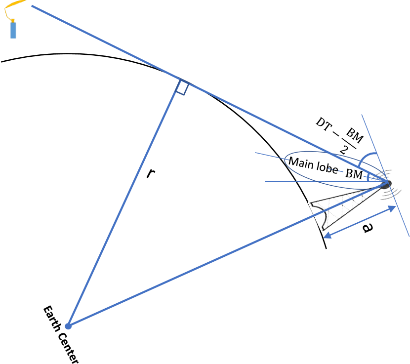
Figure 4: The impact of down-tilt angle (DT) for avoiding main-lobe interference with SMAP.

IV-D SMAP Antenna Model

As in (1), one of the key factors in evaluating interference on SMAP is its antenna gain ($G_{SMAP}$). Fig. 2 illustrates the key features of SMAP’s antenna, which includes a conically scanning golden mesh reflector measuring 6 meters in width. The 3-dB antenna beamwidth is approximately $2.4^{\circ}$ with a footprint of around $40\times 40$ km² on Earth. Additionally, an Ortho-Mode Transducer (OMT) feedhorn is employed to gather radiations from the mesh reflector and divide them into separate vertical and horizontal polarizations [41].

SMAP’s antenna gain can be expressed as the gain for vertical $G_{vv}$ and horizontal $G_{hh}$ polarizations, with extremely negligible inter-polarization $G_{hv}$ and $G_{vh}$ leakages [41]:

$$\begin{pmatrix}G_{vv}&G_{hv}\\ G_{hh}&G_{vh}\end{pmatrix}.$$ (8)

Consequently, the SMAP antenna gain for vertical polarization can be expressed as $G_{v}=G_{vv}+G_{hv}$, and for horizontal polarization can be expressed as $G_{h}=G_{hh}+G_{vh}$. Since thermal measurements are conducted independently for each polarization, SMAP antenna’s gain $G_{SMAP}$ can be determined separately for both vertical and horizontal polarizations. Fig. 5 shows a 2-dimensional cut of SMAP’s antenna gain $G$ in the restricted L-band.

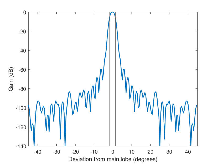
Figure 5: A 2-dimensional cut of SMAP’s conical antenna gain for the vertical polarization. The gain for the horizontal polarization is similar. The two vertical lines show the $2.4^{\degree}$ antenna beamwidth.

As can be seen in Fig. 5, SMAP’s antenna gain can be divided into two regions including i) a very sharp main lobe with gain $G_{ml}$ that has a width of approximately 2.4 degrees and ii) a sidelobe gain $G_{sl}$ with gain values as low as $-140$ dB. As a very common technique of antenna gain sectorizing in stochastic geometry [42], we assign constant values to the main and side lobes of the antenna, i.e.,

$$G_{s}=\left\{\begin{array}[]{cc}G_{ml},&\mbox{if }|d|\leq 1.2^{\degree}\\ G_{sl},&\mbox{if }|d|>1.2^{\degree},\end{array}\right.$$ (9)

where $d$ denotes the deviation from the main lobe in degrees.

In our model, we imagine that there is no RFI in the main lobe, i.e., there is no active BS on SMAP’s $40\times 40$ km² antenna footprint projected on Earth. This can be done using protocol-based precautions at each BS. Consequently, interference can only hit SMAP’s side lobe with gain $G_{sl}$, so that $G_{SMAP}=G_{sl}$ in (1).

IV-E Brightness Temperature & RFI

The signal power received by SMAP’s radiometer will be eventually interpreted as the brightness temperature. Later this brightness temperature will be interpreted as soil moisture content using different models, for example, the tau-omega model [2]. A commonly used formula for relating power to brightness temperature is the Nyquist noise formula [43]:

$$P_{s}=KBT_{s},$$ (10)

where $P_{s}$ is the signal power measured by SMAP, $K$ is the Boltzmann constant ($K=1.380649\times 10^{-23}$ m²kg s^-2K^-1), $B$ is the bandwidth ($24$ MHz in our case), and $T_{s}$ is the brightness temperature in Kelvin. For one interfering base station (BS) with interfering power $P_{RFI}^{BS}$ received at SMAP, SMAP measures the power $P_{s}=P_{soil}+P_{{\color[rgb]{0,0,0}{RFI}}}^{BS}$, where $P_{soil}$ denotes the the soil’s natural electromagnetic thermal power received from the SMAP’s antenna footprint on Earth. Consequently, the translated brightness temperature using (10) can be expressed as:

$$T_{s}=\frac{P_{soil}+P_{{\color[rgb]{0,0,0}{RFI}}}^{BS}}{KB}=T_{soil}+T_{{\color[rgb]{0,0,0}{RFI}}}^{BS},$$ (11)

where $T_{soil}$ and $T_{{\color[rgb]{0,0,0}{RFI}}}^{BS}$ denote the brightness temperatures of the soil and RFI, respectively. Considering the path loss between one cellular BS and SMAP as stated in (4), we have:

$$T_{{\color[rgb]{0,0,0}{RFI}}}^{BS}=\frac{P_{tx}A}{KB}x^{-\alpha}=\eta x^{-\alpha},$$ (12)

where we define $\eta=\frac{P_{tx}A}{KB}$ to simplify the notation. In the next subsection, we use this model of the brightness temperature of RFI for one BS ($T_{{\color[rgb]{0,0,0}{RFI}}}^{BS}$) to model the aggregate RFI brightness temperature from a large-scale terrestrial NextG network.

IV-F System Model

The notations used in this study pertaining to stochastic geometry are based on the references [28, 27]. Given that the spectrum crunch predominantly affects densely populated regions, such as metropolitan areas, we investigate the utilization of the 27 MHz wide restricted L-band for the downlink of active wireless networks in these regions. In this context, we assume that a cluster of multiple BSs serves each densely populated region. To model the interference arising from this configuration, we adopt a Thomas Poisson Cluster Process [44, 45, 46, 47], where each cluster represents a dense metropolitan area. We envision a random collection of clusters $\Phi=\{\boldsymbol{X}_{i},i\in\mathbb{N}\}$ covering the Earth’s surface, following a homogeneous Poisson Point Process (PPP) with a uniform intensity of $\lambda_{C}$ clusters per square kilometer. Within each cluster $i$, the number of active cellular BSs is modeled by a homogeneous Poisson random variable $W_{i}$ with an intensity parameter $\lambda_{BS}$ BSs per cluster. The geometry of the BSs within a cluster is not considered, as the city’s radius is much smaller than the distance to the satellite. Hence, all active BSs within a cluster are assumed to be at the same distance from the satellite.

Fig. 6 provides a 2-dimensional picture of such a scenario. In Fig. 6, at each moment, the red spherical cap is the maximum Earth’s cut exposed to SMAP, and $\psi=\arccos{(\frac{r}{h})}$ is this cut’s angle from Earth’s center, where $r$ denotes the Earth’s radius and $h$ denotes SMAP’s distance from the Earth’s center. In other words, the satellite is located at the point $\boldsymbol{y}=(0,{\color[rgb]{0,0,0}{0}},h)$. The distances $D_{\min}=h-r$ and $D_{\max}=\sqrt{h^{2}-r^{2}}$ denote the minimum and maximum possible distances between a cluster and SMAP, respectively. The grey line shows SMAP’s main beam collecting soil’s thermal radiation with gain $G_{ml}$. We assume that there are no active BSs in SMAP’s antenna footprint, i.e., no RFI hits the main lobe of SMAP’s antenna with gain $G_{ml}$. Finally, $\boldsymbol{X}_{i}$ denotes a cluster of $W_{i}$ BSs with distance $x$ to SMAP, which interfere with the side lobe of SMAP’s antenna with gain $G_{sl}$.

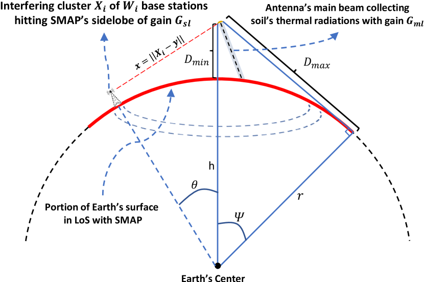
Figure 6: 2-dimensional representation of the Earth-cut exposed to the satellite. The red curve represents the maximum extent of the Earth cut exposed.

IV-G Average Interference

As mentioned earlier, we are interested in the aggregate RFI brightness temperature from all clusters $\boldsymbol{X}_{i}\in\Phi$. Using the RFI brightness temperature model defined in (12) for each BS, and using the fact that there are $W_{i}$ BSs in cluster $\mathrm{X}_{i}$, the aggregate RFI brightness temperature can be written as:

$$T_{{\color[rgb]{0,0,0}{RFI}}}=\sum_{\boldsymbol{X}_{i}\in\Phi}\eta\|\boldsymbol{X}_{i}-\boldsymbol{y}\|^{-\alpha}{\color[rgb]{0,0,0}{W_{i}}}$$ (13)

where $\|\boldsymbol{X}_{i}-\boldsymbol{y}\|$ denotes the distance from the cluster located at $\boldsymbol{X}_{i}$ to SMAP located at $\boldsymbol{y}$. The following theorem states the moment generating function (MGF) of $T_{RFI}$ in (13).

Theorem 1.

The moment generating function of $T_{{\color[rgb]{0,0,0}{RFI}}}$ in (13) with the model introduced in Section IV-F is as $M(t)=$

$$\exp\left(-\beta\int_{D_{\min}}^{D_{\max}}\left(1-\exp(\lambda_{BS}(e^{\eta tx^{-\alpha}}-1))\right)x\,dx\right)$$ (14)

with $\beta=2\pi(\frac{r}{h})\lambda_{C}$, $D_{\max}=\sqrt{h^{2}-r^{2}}$, and $D_{\min}=h-r$.

Proof.

Refer to Appendix A. ∎

Using Theorem 1, we can calculate the moments of $T_{{\color[rgb]{0,0,0}{RFI}}}$, i.e., ${\color[rgb]{0,0,0}{\mathds{E}}}[T_{{\color[rgb]{0,0,0}{RFI}}}^{n}$]. In the following Corollary, we derive the average brightness temperature induced by RFI using Theorem 1.

Corollary 1.

The average of $T_{{\color[rgb]{0,0,0}{RFI}}}$ in (13) using the RFI modeled in Section IV-F can be expressed as:

$${\color[rgb]{0,0,0}{\mu_{0}}}={\color[rgb]{0,0,0}{\mathds{E}}}[T_{{\color[rgb]{0,0,0}{RFI}}}]=\left(\frac{\beta}{2-\alpha}\right)\omega\left(D_{\max}^{2-\alpha}-D_{\min}^{2-\alpha}\right)$$ (15)

where $\omega=\eta\lambda_{BS}$.

Proof.

$\mathds{E}[T_{RFI}]$ can be acquired by taking the derivative of $M(t)$ with respect to $t$ in (14) and then setting $t=0$. ∎

Using Corollary 1, we can calculate $\mu_{0}=\mathds{E}[T_{RFI}]$, which appears as a bias on SMAP’s measurements. In the next subsection, we investigate correcting for RFI in SMAP’s measurements.

IV-H Correcting for RFI in SMAP’s measurements

The total brightness temperature $T_{s}$ measured by SMAP can be expressed as follows:

$$T_{s}=T_{soil}+T_{{\color[rgb]{0,0,0}{RFI}}},$$ (16)

where $T_{soil}$ denotes the brightness temperature of the soil and $T_{{\color[rgb]{0,0,0}{RFI}}}$ appears as a bias in the brightness temperature. If we knew the exact value of the RFI’s brightness temperature ($T_{{\color[rgb]{0,0,0}{RFI}}}$), then we could perfectly estimate the soil’s brightness temperature ($T_{soil}$) by subtracting $T_{{\color[rgb]{0,0,0}{RFI}}}$ from the measurements ($T_{s}$). However, since $T_{{\color[rgb]{0,0,0}{RFI}}}$ is a random variable with the MGF defined in Theorem 1, its value is not deterministic. One way to compensate for it is to use $\mu_{0}=\mathds{E}[T_{RFI}]$ calculated in Corollary 1 as a correction factor to estimate the soil moisture: i.e.,

$$T_{soil}=T_{s}-\mu_{0}+Err,$$ (17)

where $Err=\mu_{0}-T_{{\color[rgb]{0,0,0}{RFI}}}$. Applying this correction factor causes uncertainty ($Err$) in the estimated value of $T_{soil}$. However, most Earth exploration satellite missions can tolerate such uncertainty as long as it is below a (small) threshold. For example, SMAP can tolerate an uncertainty of $1.3$ Kelvin and SMOS can tolerate uncertainty less than a few Kelvin [11]. For this reason, we are interested in knowing the probability that $T_{{\color[rgb]{0,0,0}{RFI}}}$ differs from its mean value $\mu_{0}$ by more than a threshold $\tau$ which we call the Sensing Outage Probability (SOP), i.e., $\text{SOP}(\tau)=\mathds{P}(|T_{{\color[rgb]{0,0,0}{RFI}}}-{\color[rgb]{0,0,0}{\mu_{0}}}|>\tau)$. When considering SMAP, we are particularly interested in the case that $\tau\leq\frac{1.3}{2}=0.65$ Kelvin. To this end, we can use the general form of the Chebyshev inequality to bound the SOP:

$$\text{SOP}(\tau)\triangleq\mathds{P}\left(|T_{{\color[rgb]{0,0,0}{RFI}}}-{\color[rgb]{0,0,0}{\mu_{0}}}|>\tau\right)\leq\frac{{\color[rgb]{0,0,0}{\mathds{E}}}\left[\left(T_{{\color[rgb]{0,0,0}{RFI}}}-{\color[rgb]{0,0,0}{\mu_{0}}}\right)^{n}\right]}{\tau^{n}},$$ (18)

where $n$ has to be an even integer. Typically, we can choose $n=2$ which corresponds to $\text{Var}(T_{{\color[rgb]{0,0,0}{RFI}}})$. However, we seek higher moments of $n$ to provide tighter bounds. As observable from the right hand side of (18), to bound SOP we need to calculate the central moments of $T_{RFI}$, i.e., $\mu_{n}=\mathds{E}\left[\left(T_{{\color[rgb]{0,0,0}{RFI}}}-\mu_{0}\right)^{n}\right]$. To achieve this, we first need to introduce two key definitions.

Definition 1.

The Cumulant Generating Function (CGF) of a random variable $X$ is defined as $K_{X}(t)=\log\left({\color[rgb]{0,0,0}{\mathds{E}}}[e^{tX}]\right)=\log\left(M_{X}(t)\right)$, where $M_{X}$ is the moment generating function of $X$ [48].

Definition 2.

The $n$th cumulant of $K_{X}(t)$ is defined as [48]:

$$k_{n}=\frac{\partial^{n}}{\partial t^{n}}K_{X}(t)|_{t=0}$$ (19)

Remark 1.

For $n\in\{2,3\}$ the $n$th cumulant of $K_{X}(t)$ is equal to ${\color[rgb]{0,0,0}{\mu_{n}=\mathds{E}}}\left[\left(X-{\color[rgb]{0,0,0}{\mu_{0}}}\right)^{n}\right]$ [48].

Remark 2.

For $n=4$:

$${\color[rgb]{0,0,0}{\mu_{4}=\mathds{E}}}\left[\left(X-{\color[rgb]{0,0,0}{\mu_{0}}}\right)^{4}\right]=k_{4}+3(k_{2})^{2}$$ (20)

where $k_{i}$ is the $i$th cumulant of $K_{X}(t)$ as in (19).

With the help of the CGF and Remark 2, we can achieve a tighter bound in (18) than when $n=2$. Next, we will investigate the CGF, the cumulants, and the variance of $T_{{\color[rgb]{0,0,0}{RFI}}}$ in (13).

Corollary 2.

The cumulant generating function of $T_{{\color[rgb]{0,0,0}{RFI}}}$ in (13) can be expressed as $K_{T_{{\color[rgb]{0,0,0}{RFI}}}}(t)=$

$$-\beta\int_{D_{\min}}^{D_{\max}}\left(1-\exp(\lambda_{BS}(e^{\eta tx^{-\alpha}}-1))\right)x\,dx.$$ (21)

Proof.

According to Definition 1, $K_{T_{{\color[rgb]{0,0,0}{RFI}}}}(t)=\log\left(M(t)\right)$, where $M(t)$ is the MGF of $T_{{\color[rgb]{0,0,0}{RFI}}}$ given in Theorem 1. ∎

Using the Taylor series, we can simplify the term $e^{\eta tx^{-\alpha}}$ in (21) using the fact that $\eta$ is on the order of $10$s while $x^{-\alpha}$, with $\alpha>2$, is on the order $10^{-6}$.

Lemma 1.

Using the Taylor series, the term $e^{\eta tx^{-\alpha}}$ in (21) can be well approximated with:

$$e^{\eta tx^{-\alpha}} =1+\eta tx^{-\alpha}+\mathcal{O}^{2}(\eta tx^{-\alpha})$$

$$\approx 1+\eta tx^{-\alpha}.$$ (22)

Using (22), the CGF of $K_{T_{{\color[rgb]{0,0,0}{RFI}}}}(t)$ in Corollary 2 can be approximated as:

$$\widetilde{K}_{T_{{\color[rgb]{0,0,0}{RFI}}}}(t)=-\beta\int_{D_{\min}}^{D_{\max}}\left(1-\exp(\omega tx^{-\alpha})\right)x\,dx,$$ (23)

where $\omega=\eta\lambda_{BS}$.

Lemma 1 helps to avoid complexities in calculating the exact cumulant of $K_{T_{{\color[rgb]{0,0,0}{RFI}}}}(t)$ in (21).

Corollary 3.

Using Lemma 1, the $n$th cumulant of $\widetilde{K}_{T_{{\color[rgb]{0,0,0}{RFI}}}}(t)$ stated in (21) would be as:

$$\widetilde{k}_{n}=\left(\frac{\beta}{2-n\alpha}\right)\omega^{n}\left(D_{\max}^{(2-n\alpha)}-D_{\min}^{(2-n\alpha)}\right).$$ (24)

Proof.

Using Corollary 2 and Definition 2 we can acquire (24). ∎

Now using Corollary 3 and Remark 1, we can acquire higher moments of $\mu_{n}$ including $n=2$ that is the variance of $T_{{\color[rgb]{0,0,0}{RFI}}}$ in (13).

Corollary 4.

The variance of $T_{{\color[rgb]{0,0,0}{RFI}}}$ stated in (13) can be calculated as:

$${\color[rgb]{0,0,0}{\mu_{2}}}=\widetilde{k}_{2}=\frac{\beta}{2-2\alpha}\omega^{2}\left(D_{\max}^{(2-2\alpha)}-D_{\min}^{(2-2\alpha)}\right)$$ (25)

Proof.

The result follows from Remark 1 and Lemma 1. ∎

In Section V-B, we use the concept of cumulants to bound the SOP in (18) for different values of $\tau$.

V Simulation Results

As mentioned previously, at any given time, we partition Earth’s surface into two distinct regions. The first region, which is larger in size, corresponds to areas where SMAP is not visible in the sky. In these regions, terrestrial networks can opportunistically utilize the restricted L-band band without imposing interference on SMAP. The second region represents areas exposed to SMAP in which a terrestrial NextG network will need to implement restrictions to avoid significantly interfering with SMAP. Consequently, achieving full capacity utilization of the restricted L-band may not be feasible in these exposed regions. In the following subsections, we will explore the opportunities for spectrum coexistence between SMAP and terrestrial networks in these two regions.

V-A Opportunistic Temporal Spectrum Coexistence

To explore the potential utilization of the restricted L-band within a terrestrial NextG wireless network during SMAP’s 3-day global coverage period, we assess various factors. Specifically, we focus on a particular region on Earth and evaluate the “exposure time ratio,” which represents the proportion of SMAP’s 3-day global coverage period that SMAP is present in the sky and is exposed to the region. The orbital characteristics of SMAP’s Sun-Synchronous Orbit (SSO), as discussed in Section III-A and illustrated in Fig. 1, indicate that the latitude of the network is the primary determinant for evaluating the exposure time ratio. Furthermore, simulations indicate that longitude has minimal impact on the desired parameters mentioned earlier. We consider positive latitudes ranging from the equator ($0\degree$) to the North Pole ($90\degree$) as the results are symmetric for negative latitudes. Alongside the exposure time ratio for each latitude, we also examine the “exposure free time ratio,” which complements the exposure time ratio by indicating the duration when network is not exposed to SMAP. Additionally, we analyze the number of exposure events and the maximum exposure time over all exposure events.

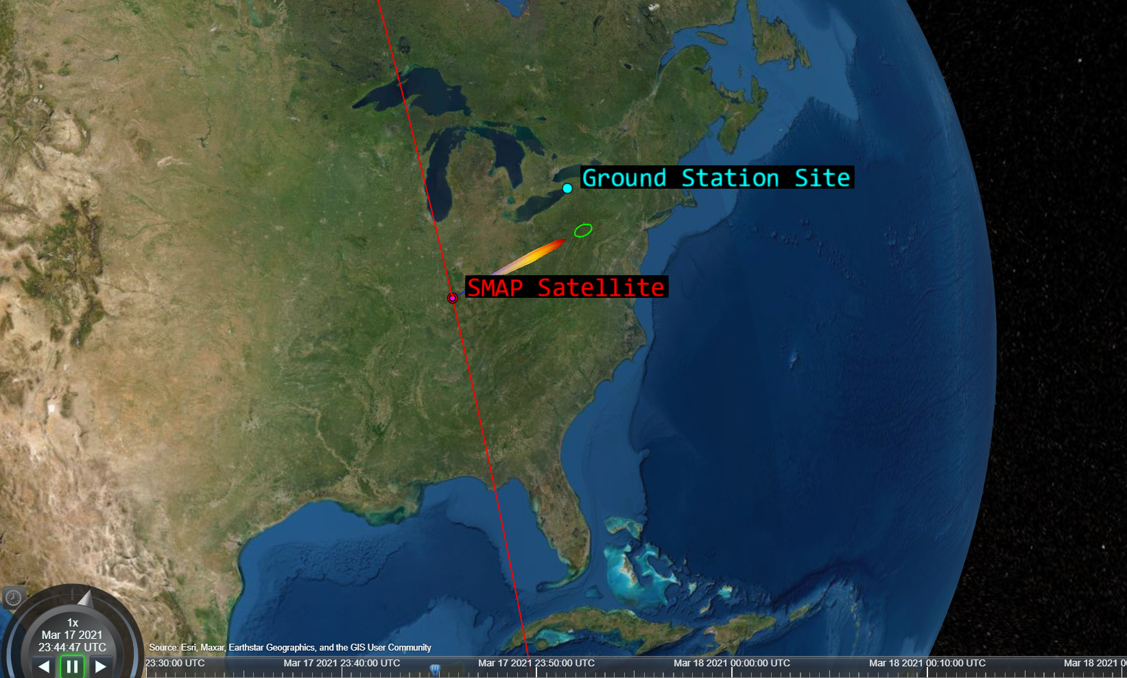
Figure 7: SMAP and a ground base station.

Table I: SSO orbital parameters of SMAP [11]

Orbital Element	Mean Element Value
Semi-major Axis (a)	7057.5071 km
Eccentricity (e)	0.0011886
Inclination (i)	98.121621 deg
Argument of Perigee (w)	90.000000 deg
Ascending Node (W)	–50.928751 deg
True Anomaly	–89.993025 deg

To conduct simulations and generate visualizations, we employ MATLAB’s SatComm library [49]. The orbital parameters for SMAP are provided in Table I, and we use two-body keplerian as our orbit propagator. A visual representation of SMAP’s orbit in conjunction with a terrestrial ground BS located in Buffalo, New York, USA is depicted in Fig. 7.

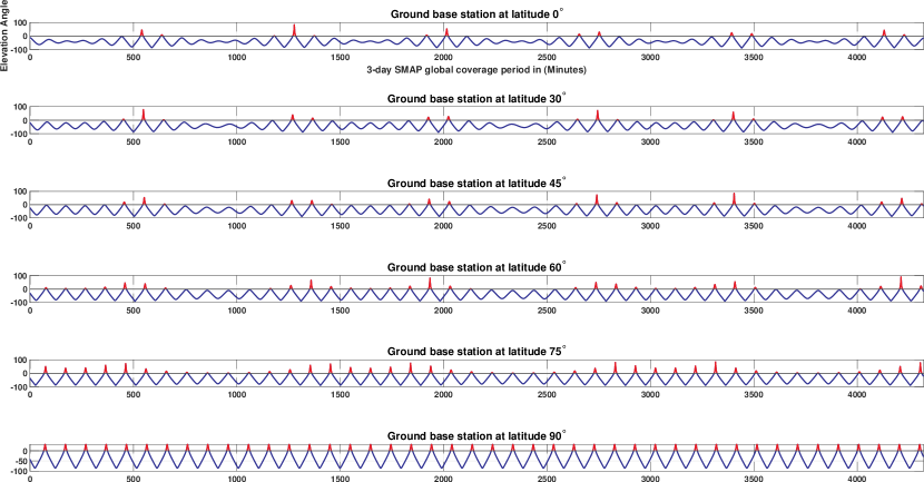
Figure 8: Elevation angle vs. time for terrestrial base station clusters at different latitudes. (Top) BS located at equator ($0\degree$ latitude). (Bottom) BS located at North Pole ($90\degree$ latitude).

As depicted in Fig. 3, exposure events occur when there is a positive elevation angle between a BS and SMAP. Conversely, for negative elevation angles, SMAP is positioned below the horizon, indicating the absence of LoS exposure to the satellite. Therefore, we take into account the angle of elevation between the terrestrial network and SMAP for various latitudes on Earth throughout SMAP’s 3-day global coverage period.

Table II: SMAP exposure statistics

Earth Latitude	Exposure Time Ratio	Exposure-Free Time Ratio	No. Exposure Events	Max. Exposure Time
$0^{\degree}$	3.18%	96.82%	13	$\sim$15 minutes
$15\degree$	3.28%	96.72%	13	$\sim$15 minutes
$30\degree$	3.74%	96.26%	15	$\sim$15 minutes
$45\degree$	4.76%	95.24%	20	$\sim$15 minutes
$60^{\degree}$	7.93%	92.07%	32	$\sim$15 minutes
$75\degree$	11.95%	88.05%	44	$\sim$15 minutes
$90\degree$	13.57%	86.43%	44	$\sim$15 minutes

In Figure 8, the elevation angles between a terrestrial BS cluster site and SMAP are depicted throughout SMAP’s 3-day global coverage period for clusters located at different latitudes, ranging from the equator ($0\degree$) to the North Pole ($90\degree$). The presence of positive elevation angles, represented by the color red, indicate exposure to SMAP. As evident from Figure 8, regions with lower latitudes exhibit extended periods without exposure, followed by intermittent bursts of short exposure events. Conversely, as the latitude angle rises, the frequency and duration of exposure events increase.

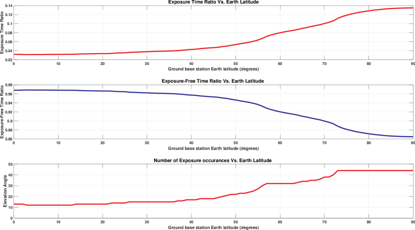
Figure 9: Exposure time ratio, exposure-free time ratio, and the number of exposure occurrences vs. terrestrial base station latitude.

The key observation derived from Fig. 8 is that, despite variations based on the latitude, SMAP is not exposed to the cluster sites for a significant portion of its 3-day global coverage period. Table II provides a summary of the results in Fig. 8. Additionally, Fig. 9 reveals more detailed insights into the exposure time ratio, exposure-free time ratio, and the number of exposure events corresponding to different latitudes.

The provided information reveals important insights regarding exposure time ratios and exposure events in relation to SMAP. Table II indicates that cluster sites at the equator exhibit a minimum exposure time ratio of $3.18\%$, resulting in a maximum exposure-free time ratio of $96.82\%$. As latitude angles increase, the exposure time ratio also rises, reaching a maximum of $13.57\%$ for cluster sites at the North Pole, which corresponds to a minimum exposure-free time ratio of $86.43\%$.

Considering exposure events is crucial due to the potential interference with SMAP. Table II and Fig. 9 provide valuable data on exposure events. Clusters situated at the equator experience a minimum of $13$ exposure events within a 3-day period, whereas polar clusters can encounter up to $44$ exposure events. Furthermore, each exposure event has a maximum duration of roughly 15 minutes. During these exposure events, clusters must either completely suspend transmissions or implement specific restrictions to avoid significant interference with SMAP.

Overall, these findings underscore that BS clusters at all latitudes have many opportunities during exposure-free times to transmit in the restricted L-band without interfering with SMAP; however, necessary precautions must be in place to ensure correct operation of SMAP and minimize potential disruptions caused by BS transmissions during exposure events. As stated in Section III, SMAP has a longer operational cycle of 8 days before returning to its initial point of operation. Our simulation results remained consistent throughout this 8-day period, so we opted to only present the results over SMAP’s 3-day global coverage period for clarity of the plots.

V-B LoS Spectrum Coexistence

In this section, we evaluate the spatial spectrum coexistence of a large-scale terrestrial network exposed to SMAP based on the stochastic geometry model described in Section III.

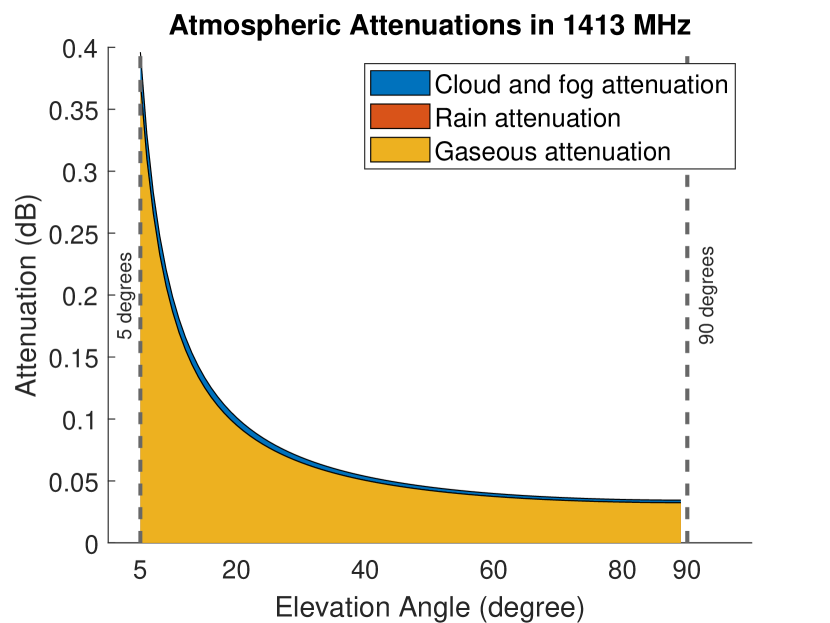
Figure 10: Attenuation due to the atmospheric gases in the 1.413 GHz frequency band.

We start by presenting the atmospheric path loss model introduced in Section IV-B. Fig. 10 shows the breakdown of atmospheric path loss in the 1413 MHz based on the elevation angle between a ground BS and SMAP. Based on [34], we can identify three major atmospheric attenuation causes in the 1.413 GHz band, that are i) Cloud and Fog attenuation, ii) Attenuation due to precipitation, and iii) Gaseous Attenuation. Also according to [34], tropospheric scintillation can be another cause for attenuation, but due to its uncertain value for frequencies below 4 GHz, we will ignore it.

Based on the information depicted in Fig. 10, the cumulative loss experienced in the 1.413 GHz frequency range due to atmospheric conditions is minimal, typically ranging from a few tenths of decibels. However, it is worth noting that at elevation angles below 5 degrees, the loss can be slightly higher. Nonetheless, we will neglect the contribution of atmospheric path loss in our model since other factors contribute more significantly to overall path loss.

Table III displays the parameters utilized in our stochastic geometry model simulation. In particular, $\lambda_{C}$ represents the average number of clusters per $10000$ km², and $\lambda_{BS}$ is the average number of active BSs per cluster. Through our model, established in Section III, we observe that the average RFI brightness temperature and the standard deviation of RFI brightness temperature have a nearly linear relationship with $\lambda_{C}$. Hence, we focus our performance analysis on a single value of $\lambda_{C}$, and 4 different values of $\lambda_{BS}$, which are outlined in Table III. By setting the value of $\lambda_{C}$ to 1 cluster per $10000$ km², we anticipate an approximate average of $2500$ active clusters within the section of the Earth that is visible to SMAP at any given time.

Table III: LIST OF CONFIGURATION PARAMETERS FOR PERFORMANCE EVALUATION

Element	Value
Intensity of clusters ($\lambda_{C}$)	$1$ cluster (large city) every $10000$ $km^{2}$
Intensity of active BS ($\lambda_{BS}$)	$100$, $600$, $1200$, $2000$ BSs per cluster
Exponent Path Loss ($\alpha$)	[2.1 , 2.5]
BS transmission power ($P_{tx}$)	$35$ dBm $3.164$ Watts per BS
SMAP’s sidelobe antenna gain ($G_{SMAP}$)	$-40$ dB
BS sidelobe antenna gain ($G_{BS}$)	$-15$ dB
Central Carrier frequency of BS ($f$)	$1.413$ GHz
Noise power in terrestrial environment ($\sigma^{2}$)	$-174$ dBm/Hz
BS transmission bandwidth ($B$)	$24$ MHz
Earth radius ($r$)	$6371$ km
SMAP’s distance to Earth’s center ($h$)	$7056$ km
Min. possible distance to SMAP ($D_{\min}$)	$h-r=685$ km
Max. possible distance to SMAP ($D_{\max}$)	$\sqrt{h^{2}-r^{2}}=3032.7$ km
Max. possible value of $\theta$ ($\psi$)	$\arccos(\frac{r}{h})=0.4443$ rad

Initially, we employ Corollary 1 to assess the mean RFI brightness temperature induced on SMAP by a terrestrial NextG network characterized by the parameters in Table III. Fig. 11 displays the average brightness temperature for a terrestrial network comprising an average of $\lambda_{BS}=100$ to $2000$ BSs per cluster, utilizing an exponential path loss model with parameter $\alpha\in[2.1,2.5]$. The findings reveal that the highest brightness temperature recorded is below $7$ Kelvin, observed when clusters feature an average of $\lambda_{BS}=2000$ active BSs. Conversely, the lowest brightness temperature observed is below $1$ Kelvin for clusters composed of an average of $\lambda_{BS}=100$ BSs. Additionally, it is evident that the brightness temperature experiences a significant decrease with increasing values of the path loss exponent $\alpha$.

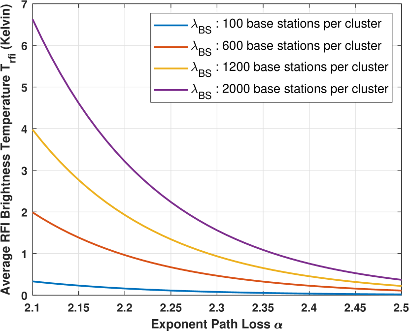
Figure 11: Average RFI brightness temperature

The crucial aspect to highlight is that when dealing with networks containing over 1 million active BSs (specifically, clusters with more than $\lambda_{BS}=400$ active BSs), the resulting RFI brightness temperature exceeds $1.3$ Kelvin, which surpasses the maximum allowable error in measurements as per legal standards. Consequently, our focus will now shift towards mitigating the impact of RFI utilizing the models elaborated in Section IV-H.

As mentioned in (17), addressing the influence of the brightness temperature $T_{RFI}$ entails subtracting its average value $\mathds{E}[T_{RFI}]$ from measurements. To accomplish this effectively, it becomes crucial to assess how accurately the average brightness temperature $\mathds{E}[T_{RFI}]$ represents the true value of the random variable $T_{RFI}$. A key factor in this evaluation is the concentration of $T_{RFI}$ around its mean value. Consequently, we employ the standard deviation as a metric to gauge this concentration. To calculate the brightness temperature, we use Corollary 4 in Section IV-H.

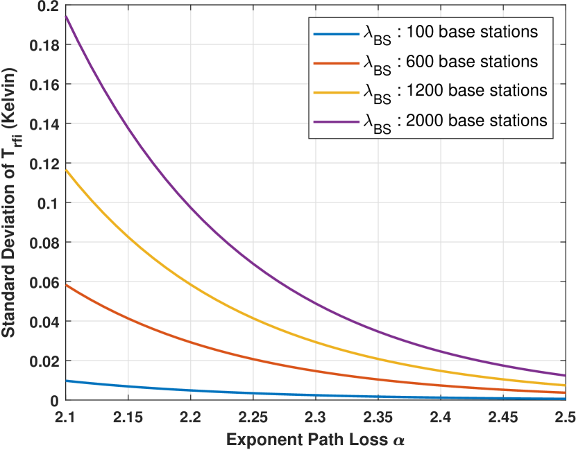
Figure 12: Standard Deviation of RFI brightness temperature.

Fig. 12 illustrates the standard deviation of the RFI brightness temperature induced by a network with the same parameters as in Table III, wherein the average number of active BSs per cluster ranges from $\lambda_{BS}=100$ to $2000$. The graph provides valuable insights: when considering a network with an average of $\lambda_{BS}=2000$ active BSs per cluster, the standard deviation of the RFI brightness temperature remains below $0.2$ Kelvin. Moreover, for clusters with a lower number of active BSs per cluster, the standard deviation is even lower. From this analysis, we can conclude that the induced RFI brightness temperature exhibits a high level of concentration around its mean value. This finding further supports the feasibility of mitigating the impact of RFI on SMAP’s measurements by deducting the average RFI brightness temperature as a correction factor as proposed in (17).

In addition to having a low standard deviation, it is essential to ensure that, after applying the correction factor, the error in SMAP’s measured brightness temperature remains below certain thresholds. To achieve this, we assess the sensing outage probability, i.e., $SOP(\tau)$ defined in (18), for different threshold values $\tau$ across different network configurations. In (18), we choose $n=4$. This allows us to establish reliable estimates and insights regarding the likelihood of surpassing the defined threshold values, aiding in the development of appropriate measures to mitigate potential errors after applying the correction factor.

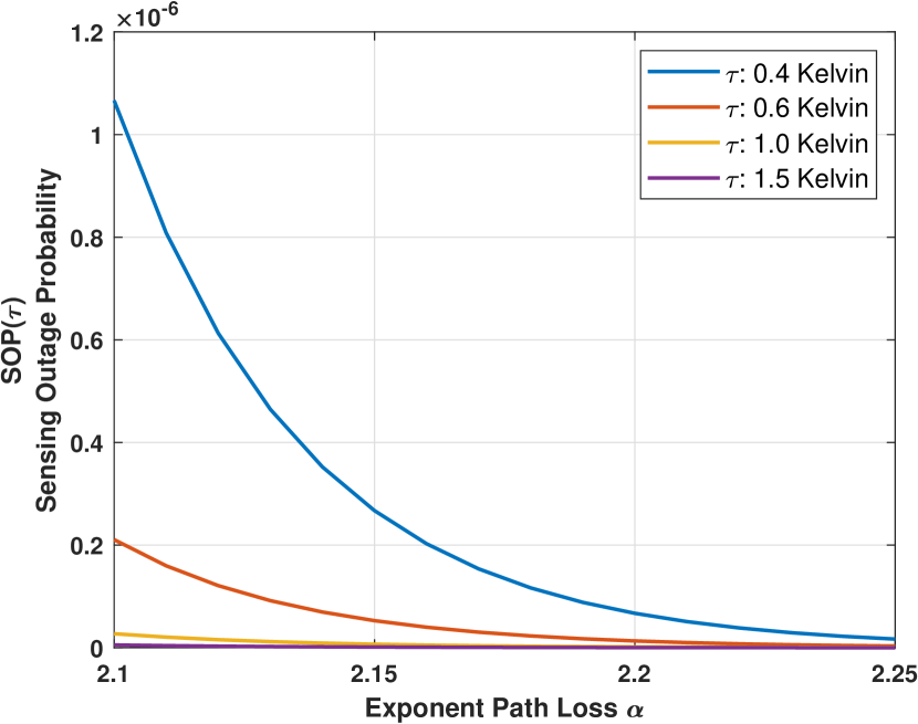
(a) $\lambda_{BS}=100$ (247,587 BSs exposed to SMAP on average).

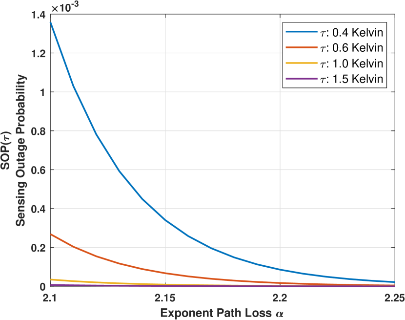
(b) $\lambda_{BS}=600$ (1,485,520 BSs exposed to SMAP on average).

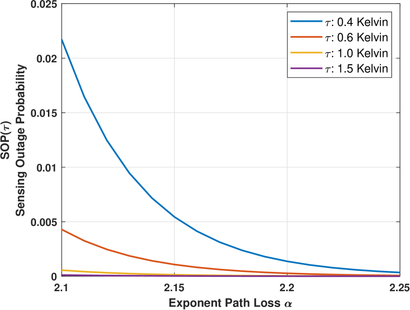
(c) $\lambda_{BS}=1200$ (2,971,039 BSs exposed to SMAP on average).

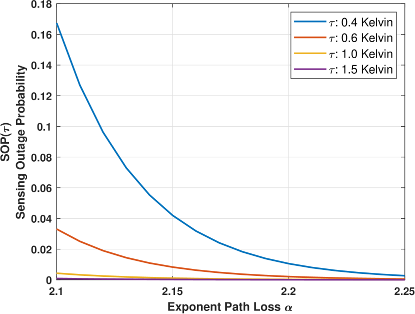
(d) $\lambda_{BS}=2000$ (4,951,732 BSs exposed to SMAP on average).

Figure 13: SOP($\tau$) for different values of $\tau$ and $\lambda_{BS}$.

Fig. 13 displays $SOP(\tau)$ associated with various threshold values, namely $\tau=0.4$, $0.6$, $1.0$, and $1.5$ Kelvin, across different numbers of active BSs per cluster. The graph provides insights into the likelihood of surpassing these threshold values and allows for a comprehensive analysis of the impact of different cluster configurations on the RFI brightness temperature. In the top-left plot, it is evident that the probability of error surpassing the threshold $\tau=0.4$ measures less than $1.2\times 10^{-6}$. This extremely small value, approaching zero, indicates that the RFI brightness temperature $T_{RFI}$ is highly concentrated around its mean value. This finding holds true for a network of clusters with an average of $\lambda_{BS}=100$ active BSs per cluster, which corresponds to around 250,000 active BSs on the earth cut exposed to SMAP. Furthermore, by observing the other plots, it becomes apparent that the probability of exceeding the error threshold increases with the number of active BSs per cluster. Notably, for clusters with $\lambda_{BS}=2000$ active BSs, the probability of error exceeding the threshold can reach as high as $20\%$. This indicates a greater level of uncertainty and dispersion in the RFI brightness temperature measurements for networks with larger cluster sizes. Lastly, regardless of the cluster size $\lambda_{BS}$ and threshold $\tau$, $SOP(\tau)$ decays exponentially as the path loss exponent $\alpha$ increases. In all illustrated scenarios, $SOP(\tau)$ is less than $5\%$ for $\alpha>2.15$.

The comprehensive findings indicate that a large-scale terrestrial NextG wireless network can coexist harmoniously with SMAP within the restricted L-band. Furthermore, the detrimental effects of RFI can be effectively mitigated. As a result, it is possible to achieve a notably improved spectral efficiency within this 27 MHz passive band. This outcome highlights the potential for enhanced performance and efficiency in utilizing the allocated frequency spectrum for both passive sensing devices and active wireless systems.

VI Conclusion

Immense pressure on the frequency spectrum due to the spectrum crunch has urged researchers to investigate the coexistence of active and passive systems in the restricted passive frequency bands, such as the $1.400$ to $1.427$ GHz restricted L-band that is used by many modern earth exploration satellites. In this paper, we examined spectrum coexistence with NASA’s SMAP satellite which is one the latest remote sensing satellites that operates in this band. We explored spectrum coexistence with SMAP in two different means. First, based on SMAP’s orbital characteristics, we investigated a temporal opportunistic approach using SMAP’s absence periods for wireless transmissions within a terrestrial network using the restricted band. We demonstrated that the ratio of time available for transmission using this opportunistic approach depends on the Earth latitude of a terrestrial network’s site, and is around $96\%$ for Earth’s latitude near the equator and around $86\%$ for a network site on the Earth’s poles. We also investigated the feasibility of a large-scale terrestrial network in the LoS of SMAP satellite active in this restricted band using stochastic geometry. Using cluster processes, we modeled dense urban areas as clusters, where within each cluster multiple cellular base stations can be active in this restricted band. We modeled the RFI imposed on the SMAP satellite from such a large terrestrial network and managed to calculate the average RFI imposed on SMAP. In the next step, we demonstrated that RFI appears as a bias value added with SMAP measurements, and has to be subtracted from the measurements. For this purpose, we deployed probability concentration bounds to demonstrate how the expected value of RFI represents the real value of RFI. In general, we evaluated the RFI model with around $2500$ clusters with up to around $5$ million active cells.

Appendix A Proof of Theorem 1

According to the definition, the moment generating function of $T_{{\color[rgb]{0,0,0}{RFI}}}$ defined in (13) will be:

$$M(t) ={\color[rgb]{0,0,0}{\mathds{E}}}\left[e^{tT_{{\color[rgb]{0,0,0}{RFI}}}}\right]$$

$$={\color[rgb]{0,0,0}{\mathds{E}}}_{\Phi,\{{\color[rgb]{0,0,0}{W_{i}}}\}}\left[\prod_{\mathrm{X}_{i}\in\Phi}\exp\left(\eta\|\mathrm{X}_{i}-\mathtt{y}\|^{-\alpha}t{\color[rgb]{0,0,0}{W_{i}}}\right)\right]$$ (26)

Due to the initial assumption of the independence of the clusters $W_{i}$, we move the expectation with respect to $W_{i}$ inside the product as:

$$M(t)={\color[rgb]{0,0,0}{\mathds{E}}}_{\Phi}\left[\prod_{\mathrm{X}_{i}\in\Phi}{\color[rgb]{0,0,0}{\mathds{E}}}_{{\color[rgb]{0,0,0}{W}}}\left[\exp\left(\eta\|\mathrm{X}_{i}-\mathtt{y}\|^{-\alpha}t{\color[rgb]{0,0,0}{W}}\right)\right]\right]$$ (27)

With the knowledge that $W$ is a Poisson random variable, the expression ${\color[rgb]{0,0,0}{\mathds{E}}}_{{\color[rgb]{0,0,0}{W}}}[\exp(\cdot)]$ is the moment generating function of a Poisson random variable with parameter $\lambda_{BS}$, as defined in Section IV-F. Consequently, we have

$$M(t)={\color[rgb]{0,0,0}{\mathds{E}}}_{\Phi}\left[\prod_{\mathrm{X}_{i}\in\phi}\exp(\lambda_{BS}(e^{\eta t\|\mathrm{X}_{i}-\mathtt{y}\|^{-\alpha}}-1))\right]$$ (28)

By defining $g(\mathrm{X}_{i})=\exp(\lambda_{BS}(e^{\eta t\|\mathrm{X}_{i}-\mathtt{y}\|^{-\alpha}}-1))$, and with the knowledge that $\mathrm{X}_{i}\in\Phi$, where $\Phi$ is a homogeneous PPP with intensity $\lambda_{C}$, the expression ${\color[rgb]{0,0,0}{\mathds{E}}}_{\Phi}[\cdot]$ in (28) is the Probability Generating Functional (PGFL) [28, 27] of the function $g(\mathrm{X}_{i})$, i.e.,

$$\small\mathcal{P}_{\Phi}(g)={\color[rgb]{0,0,0}{\mathds{E}}}_{\Phi}\left[\prod_{\mathrm{X}_{i}\in\Phi}g(\mathrm{X}_{i})\right]=\exp\left(-\lambda_{C}\int_{\mathbb{R}^{d}}\left(1-g(\mathtt{x})\right)\,d\mathtt{x}\right)$$ (29)

where $\mathbb{R}^{{\color[rgb]{0,0,0}{2}}}$ in (29) is the Earth cut area exposed to SMAP as shown by the red curve in Fig. 6. $\|\mathtt{x}-\mathtt{y}\|$ is the distance of point $\mathtt{x}$ on the Earth’s surface to SMAP at point $\mathtt{y}$, and in terms of angle $\theta$ (in Fig. 6) and by using the law of cosines is as:

$$x=\left(r^{2}+h^{2}-2hr\cos(\theta)\right)^{\frac{1}{2}}$$ (30)

with:

$$dx=hr\sin(\theta)\left(r^{2}+h^{2}-2hr\cos(\theta)\right)^{-\frac{1}{2}}\;d\theta$$

$$\Rightarrow x\; dx=hr\sin(\theta)\;d\mathtt{\theta}$$ (31)

Also, $d\mathtt{x}$ in (29) is the differentiation of the area. Transforming into Spherical coordinate $\mathtt{x}=(\theta,\phi)$, using the fact that sphere area covered in $[0,\theta]$ is as $2\pi r^{2}(1-\cos(\theta))$, the differentiation of area with respect to $\theta$ would be as:

$$d\mathtt{x}=2\pi r^{2}\sin(\theta)\,d\theta$$ (32)

To write the whole integral in (29) in terms of $x$ as in (30), using (31) and (32), we note that

$$d\mathtt{x}=2\pi\left(\frac{r}{h}\right)x\;dx$$ (33)

As $x$ in (30) is the distance to the satellite, according to Fig. 6, $x$ can vary from $D_{\min}$ to $D_{\max}$. Finally, by substituting $x$ and $d\mathtt{x}$ to (29), we reach to (14).

References

- [1] J. B. Campbell and R. H. Wynne, Introduction to remote sensing. Guilford Press, 2011.
- [2] D. Entekhabi, E. G. Njoku, P. E. O’Neill, K. H. Kellogg, W. T. Crow, W. N. Edelstein, J. K. Entin, S. D. Goodman, T. J. Jackson, J. Johnson et al., “The soil moisture active passive (smap) mission,” Proceedings of the IEEE, vol. 98, no. 5, pp. 704–716, 2010.
- [3] P. O’Neill, R. Bindlish, S. Chan, E. Njoku, and T. Jackson, “Algorithm theoretical basis document. level 2 & 3 soil moisture (passive) data products,” 2018.
- [4] N. R. Council et al., Handbook of Frequency Allocations and Spectrum Protection for Scientific Uses. National Academies Press, 2007.
- [5] J. A. Hurtado Sánchez, K. Casilimas, and O. M. Caicedo Rendon, “Deep reinforcement learning for resource management on network slicing: A survey,” Sensors, vol. 22, no. 8, p. 3031, 2022.
- [6] D. C. Sicker and L. Blumensaadt, “The wireless spectrum crunch: White spaces for 5g?” Fundamentals of 5G Mobile Networks, pp. 165–189, 2015.
- [7] M. Polese, X. Cantos-Roman, A. Singh, M. J. Marcus, T. J. Maccarone, T. Melodia, and J. M. Jornet, “Coexistence and spectrum sharing above 100 ghz,” arXiv preprint arXiv:2110.15187, 2021.
- [8] Y. H. Kerr, P. Waldteufel, J.-P. Wigneron, J. Martinuzzi, J. Font, and M. Berger, “Soil moisture retrieval from space: The soil moisture and ocean salinity (smos) mission,” IEEE transactions on Geoscience and remote sensing, vol. 39, no. 8, pp. 1729–1735, 2001.
- [9] D. M. Le Vine, G. S. Lagerloef, F. R. Colomb, S. H. Yueh, and F. A. Pellerano, “Aquarius: An instrument to monitor sea surface salinity from space,” IEEE Transactions on Geoscience and Remote Sensing, vol. 45, no. 7, pp. 2040–2050, 2007.
- [10] D. Entekhabi, S. Yueh, P. E. O’Neill, K. H. Kellogg, A. Allen, R. Bindlish, M. Brown, S. Chan, A. Colliander, W. T. Crow et al., “Smap handbook–soil moisture active passive: Mapping soil moisture and freeze/thaw from space,” 2014.
- [11] D. Entekhabi et al., “SMAP handbook–soil moisture active passive: Mapping soil moisture and freeze/thaw from space,” 2014.
- [12] M. Koosha and N. Mastronarde, “Opportunistic temporal spectrum coexistence of passive radiometry and active wireless networks,” in 2022 IEEE Western New York Image and Signal Processing Workshop (WNYISPW), 2022, pp. 1–4.
- [13] M. Zheleva, C. R. Anderson, M. Aksoy, J. T. Johnson, H. Affinnih, and C. G. DePree, “Radio dynamic zones: Motivations, challenges, and opportunities to catalyze spectrum coexistence,” IEEE Communications Magazine, 2023.
- [14] Y. R. Ramadan, H. Minn, and Y. Dai, “A new paradigm for spectrum sharing between cellular wireless communications and radio astronomy systems,” IEEE Transactions on communications, vol. 65, no. 9, pp. 3985–3999, 2017.
- [15] D.-H. Jung, J.-G. Ryu, W.-J. Byun, and J. Choi, “Performance analysis of satellite communication system under the shadowed-rician fading: A stochastic geometry approach,” IEEE Transactions on Communications, vol. 70, no. 4, pp. 2707–2721, 2022.
- [16] X. Han, L. Zhang, X. Yan, K. Chen, J. Min, C. Su, and Z. Feng, “A tractable approach to coexistence analysis between compass and td-lte system,” in 2014 21st International Conference on Telecommunications (ICT). IEEE, 2014, pp. 77–81.
- [17] C. Zhang, C. Jiang, L. Kuang, J. Jin, Y. He, and Z. Han, “Spatial spectrum sharing for satellite and terrestrial communication networks,” IEEE Transactions on Aerospace and Electronic Systems, vol. 55, no. 3, pp. 1075–1089, 2019.
- [18] I. Latachi, M. Karim, A. Hanafi, T. Rachidi, A. Khalayoun, N. Assem, S. Dahbi, and S. Zouggar, “Link budget analysis for a leo cubesat communication subsystem,” in 2017 International Conference on Advanced Technologies for signal and image processing (ATSIP). IEEE, 2017, pp. 1–6.
- [19] E. Del Re, F. Argenti, L. Ronga, T. Bianchi, and R. Suffritti, “Power allocation strategy for cognitive radio terminals,” in 2008 First International Workshop on Cognitive Radio and Advanced Spectrum Management. IEEE, 2008, pp. 1–5.
- [20] A. Khawar, I. Ahmad, and A. I. Sulyman, “Spectrum sharing between small cells and satellites: Opportunities and challenges,” in 2015 IEEE International Conference on Communication Workshop (ICCW). IEEE, 2015, pp. 1600–1605.
- [21] J. Janhunen, J. Ketonen, A. Hulkkonen, J. Ylitalo, A. Roivainen, and M. Juntti, “Satellite uplink transmission with terrestrial network interference,” in 2015 IEEE global communications conference (GLOBECOM). IEEE, 2015, pp. 1–6.
- [22] P. N. Mohammed and J. R. Piepmeier, “Microwave radiometer rfi detection using deep learning,” IEEE Journal of Selected Topics in Applied Earth Observations and Remote Sensing, vol. 14, pp. 6398–6405, 2021.
- [23] A. Owfi and F. Afghah, “Autoencoder-based radio frequency interference mitigation for smap passive radiometer,” arXiv preprint arXiv:2304.13158, 2023.
- [24] Z. Khan, J. J. Lehtomaki, R. Vuohtoniemi, E. Hossain, and L. A. DaSilva, “On opportunistic spectrum access in radar bands: Lessons learned from measurement of weather radar signals,” IEEE Wireless Communications, vol. 23, no. 3, pp. 40–48, 2016.
- [25] S.-S. Raymond, A. Abubakari, and H.-S. Jo, “Coexistence of power-controlled cellular networks with rotating radar,” IEEE Journal on Selected Areas in Communications, vol. 34, no. 10, pp. 2605–2616, 2016.
- [26] D. Entekhabi et al., “The soil moisture active/passive mission (SMAP),” in IGARSS 2008-2008 IEEE International Geoscience and Remote Sensing Symposium, vol. 3, 2008, pp. III–1.
- [27] J. G. Andrews, A. K. Gupta, and H. S. Dhillon, “A primer on cellular network analysis using stochastic geometry,” arXiv preprint arXiv:1604.03183, 2016.
- [28] F. Baccelli and B. Błaszczyszyn, “Stochastic geometry and wireless networks: Volume i theory,” Foundations and Trends® in Networking, vol. 3, no. 3–4, pp. 249–449, 2010. [Online]. Available: http://dx.doi.org/10.1561/1300000006
- [29] ——, “Stochastic geometry and wireless networks: Volume ii applications,” Foundations and Trends® in Networking, vol. 4, no. 1–2, pp. 1–312, 2010. [Online]. Available: http://dx.doi.org/10.1561/1300000026
- [30] M. Haenggi, Stochastic geometry for wireless networks. Cambridge University Press, 2012.
- [31] D. Campos, L.-G. Guerrero-Ojeda, V. Alarcon-Aquino, and D. Baez-Lopez, “Satellite-indoor mobile communications path propagation losses,” in 16th International Conference on Electronics, Communications and Computers (CONIELECOMP’06). IEEE, 2006, pp. 4–4.
- [32] I. ITU-R, “Attenuation by atmospheric gases and related effects,” International Telecommunication Union-Recommendation, pp. 676–12, 2019.
- [33] Q. Wu, D. W. Matolak, and R. D. Apaza, “Airport surface area propagation path loss in the vhf band,” in 2011 Integrated Communications, Navigation, and Surveillance Conference Proceedings. IEEE, 2011, pp. B4–1.
- [34] ITU-R, “Propagation data required for the evaluation of interference between stations in space and those on the surface of the Earth,” International Telecommunication Union - Radiocommunication Sector, Geneva, Switzerland, Tech. Rep. ITU-R P 619.5, 2019.
- [35] International Telecommunication Union, “Attenuation by atmospheric gases,” ITU-R, Geneva, Switzerland, Tech. Rep. P.676-11, 2018.
- [36] ——, “Water vapour: surface density and total columnar content,” ITU-R, Geneva, Switzerland, Tech. Rep. P.836-7, 2017.
- [37] ——, “Ionospheric propagation data and prediction methods required for the design of satellite networks and systems,” ITU-R, Geneva, Switzerland, Tech. Rep. P.531-14, 2016.
- [38] E. Benner and A. B. Sesay, “Effects of antenna height, antenna gain, and pattern downtilting for cellular mobile radio,” IEEE Transactions on Vehicular Technology, vol. 45, no. 2, pp. 217–224, 1996.
- [39] J. Niemela and J. Lempiainen, “Impact of mechanical antenna downtilt on performance of wcdma cellular network,” in 2004 IEEE 59th Vehicular Technology Conference. VTC 2004-Spring (IEEE Cat. No.04CH37514), vol. 4, 2004, pp. 2091–2095 Vol.4.
- [40] J. Niemelä, T. Isotalo, and J. Lempiäinen, “Optimum antenna downtilt angles for macrocellular wcdma network,” EURASIP Journal on Wireless Communications and Networking, vol. 2005, pp. 1–12, 2005.
- [41] J. Piepmeier, P. Mohammed, G. De Amici, E. Kim, J. Peng, C. Ruf, M. Hanna, S. Yueh, and D. Entekhabi, “Soil moisture active passive (smap) project algorithm theoretical basis document smap l1b radiometer data product: L1b_tb,” Tech. Rep., 2016.
- [42] S. Wu, R. Atat, N. Mastronarde, and L. Liu, “Improving the coverage and spectral efficiency of millimeter-wave cellular networks using device-to-device relays,” IEEE Transactions on Communications, vol. 66, no. 5, pp. 2251–2265, 2018.
- [43] C. S. Turner, “Johnson-nyquist noise,” url: http://www. claysturner. com/dsp/Johnson-NyquistNoise, 2012.
- [44] C. Saha, M. Afshang, and H. S. Dhillon, “Poisson cluster process: Bridging the gap between ppp and 3gpp hetnet models,” in 2017 Information Theory and Applications Workshop (ITA). IEEE, 2017, pp. 1–9.
- [45] M. Afshang, H. S. Dhillon, and P. H. J. Chong, “Modeling and performance analysis of clustered device-to-device networks,” IEEE Transactions on Wireless Communications, vol. 15, no. 7, pp. 4957–4972, 2016.
- [46] Y. J. Chun, M. O. Hasna, and A. Ghrayeb, “Modeling heterogeneous cellular networks interference using poisson cluster processes,” IEEE Journal on Selected Areas in Communications, vol. 33, no. 10, pp. 2182–2195, 2015.
- [47] M. Afshang and H. S. Dhillon, “Spatial modeling of device-to-device networks: Poisson cluster process meets poisson hole process,” in 2015 49th Asilomar Conference on Signals, Systems and Computers. IEEE, 2015, pp. 317–321.
- [48] G.-C. Rota and J. Shen, “On the combinatorics of cumulants,” Journal of Combinatorial Theory, Series A, vol. 91, no. 1-2, pp. 283–304, 2000.
- [49] The MathWorks, “MATLAB and Satellite Communications Toolbox.” [Online]. Available: https://www.mathworks.com/products/satellite-communications.html