A systematic search for double eclipsing binaries in Zwicky Transient Facility data

Abstract

Context. Double eclipsing binaries are gravitationally bound quadruple systems in a ‘2+2’ configuration where both of the binaries are eclipsing. These systems are interesting objects to better understand stellar formation, to investigate the dynamical interaction between the two binary systems or to study certain stages of stellar evolution, such as common-envelope events or Type Ia Supernovae.

Aims. With this work, we aim to determine if double eclipsing binaries can be found using ZTF data and what the difficulties are in doing so. Secondly, we aim to significantly increase the number of known double eclipsing systems and determine how this sample differs from samples of double eclipsing binaries found with other telescopes.

Methods. We develop a new method to systematically search for double eclipsing binaries in sparsely sampled light curves. For this we use box-least-squares (BLS) to search for the period of the first binary in the system. We then remove that signal from the light curves, and search the residual light curve again with BLS to find the second period. We applied this method to ZTF light curves of 575 526 eclipsing binaries known in the Gaia eclipsing binary catalogue.

Results. We report the discovery of 198 new double eclipsing binary systems. The shortest and longest orbital periods of the newly detected systems are 0.11 days to 323 days respectively.

Conclusions. We successfully implemented a method that systematically searches for double eclipsing binary systems in sparsely sampled data. In total 198 new double eclipsing binary systems have been found in 575 526 light curves ($\approx$ 0.034$\%$). The ZTF sample typically contains more short period binaries compared to the TESS sample, but is also able to find systems with longer periods than what is currently known. We expect that at least three to four times more quadruples can be found by applying this method to all ZTF stellar light curves, by increasing the number of data points as a result of longer observations, and by implementing an automatic detection mechanism that replaces visual inspection.

1 Introduction

Most stars in the Universe can be found in gravitationally bound binaries or higher-order hierarchies (Tokovinin, 2014). It is estimated that approximately $4\%$ of all solar-type stars can be found in quadruple systems (Tokovinin, 2021), either in a 3+1 or 2+2 configuration. A small fraction of 2+2 quadruple systems are double eclipsing binaries, in which two eclipsing binaries also orbit each other (Zasche et al., 2019). If the motion of the inner pair is not strongly perturbed by the outer companions, the motions of the stars are approximated by stable Keplerian orbits and can survive for a long time (Tokovinin, 2014).

Compact double eclipsing binaries are interesting objects of study to better understand stellar formation or to investigate the dynamical interaction between the two binary systems. An important example of such a dynamical interaction is the Kozai-Lidov mechanism where, on long timescales, a periodic exchange between the binaries’ eccentricities and inclination can take place (Kozai, 1962; Lidov, 1962). Furthermore, these objects serve as an astrophysical laboratory when studying certain stages of stellar evolution, such as common-envelope events or Type Ia Supernovae (Kostov et al., 2022a). Therefore, the identification of more double eclipsing binaries will lead to a larger sample that can be used to study the origin and life cycle of these objects. Quadruples are intrinsically rare and require a favourable alignment of both binaries with the observer in order to be detected. However, in the case of fortunate alignment, the objects can be identified by periodic eclipses in the light curve. Zasche et al. (2019) systematically searched the OGLE-LMC data by visually inspecting the light curves of eclipsing binary systems and found 72 systems of double eclipsing binaries. More recently, light curves of the Transient Exoplanet Survey Satellite (TESS, Ricker et al. 2015) have been used to identify double eclipsing binaries in this way. Zasche et al. (2022b) identified 116 double eclipsing binaries using TESS, and Kostov et al. (2022a, b) detected in total 199 double eclipsing binaries, 18 of which overlapped with Zasche et al. (2022b).

In this paper, we present the search for double eclipsing binaries in Zwicky Transient Facility light curves. In Sect. 2 we present the target preselection and the ZTF data. In Sect. 3 we discuss the method we used to identify double eclipsing binaries. In Sect. 4 we present the analysis of the data. The results are presented in Sect. 5 and we discuss them further in Sect. 6. We end the paper with a summary and recommendations for future work in Sect. 7.

2 Data

As part of the Zwicky Transient Facility (ZTF), the Palomar 48-inch (P48) telescope has been imaging the sky every night since 2018 (Graham et al., 2019; Bellm et al., 2019; Dekany et al., 2020). Most of the time, ZTF uses the $g$ and $r$ bands, but a small fraction of the observations are also made in the $i$ band. The exposure times are predominantly 30 seconds for $g$ and $r$ and 60 or 90 seconds for $i$ exposures. The median limiting magnitude, averaged over the lunar cycle, is $\approx 20.5$ in all three bands. We used the PSF-photometry-based light curves which are automatically generated for all persistent sources detected in the ZTF reference images (for a full description see Masci et al., 2019) and are publicly available.

In order to avoid searching billions of ZTF light curves, we make a preselection of objects. We process only light curves of objects that have been identified as eclipsing binaries by Gaia (Mowlavi et al., 2023). Although this preselection inevitably means that we will miss any system that has not been identified as an eclipsing star by Gaia first, the advantage is that it strongly reduces the number of light curves we need to search.

The Gaia eclipsing binary catalogue contains 2 184 477 sources distributed over the whole sky and down to magnitude $G\approx 20.5$. While ZTF goes slightly deeper than Gaia, ZTF only covers the sky from the celestial north pole to a declination of $-30\deg$. This means there are 1 210 001 sources in the Gaia eclipsing binary catalogue that are also in the ZTF footprint and are fainter than $G=12$ (the approximate ZTF saturation limit). To download ZTF light curves for these objects, we used ZTFquery (Rigault, 2018).

3 Method

Light curves of double eclipsing binaries contain the signal of two eclipsing binaries with different periods. If the light curve is well sampled (e.g. the continuous light curves of TESS), multiple epochs sample each individual eclipse and the individual eclipses are easy to identify. This makes the identification of double eclipsing binaries relatively straightforward (Zasche et al., 2019; Kostov et al., 2022a; Zasche et al., 2022a). However, if a light curve is sparsely sampled (the typical time between observations is much larger than the duration of an eclipse) individual eclipses are sampled by a few or just a single epoch only and the light curve needs to be phase-folded in order to identify eclipses. Therefore, searching for double eclipsing binaries requires a slightly different approach for sparsely sampled light curves like ZTF. Instead of identifying individual eclipses, we use the fact that both eclipse signals are periodic and use period-finding methods to identify both periods.

We implemented this method using box-least-squares (BLS, Kovács et al., 2002) which is available through the Python package Astrobase (Bhatti et al., 2017). First the data from the different bands ($g$ and $r$) were combined by normalising the data in each band to its corresponding mean. Then we performed the BLS period search on the light curve to find the first period, which we define as period A. In our experience, this period was often half the orbital period and thus the primary and secondary eclipse overlapped. To avoid this overlap, we phase-folded the light curve to twice period A. To remove the signal of period A, we binned the phase-folded light curve using an empirically determined number of 100 bins. We then divided each flux measurement in the light curve by the mean of its corresponding bin. After the removal of the signal at period A, we applied the BLS method again to find the second period; period B. At each point in this process, we saved the phase-folded and binned light curves for visual inspection. An example of a (phase-folded) light curve can be seen in Fig. 1.

4 Analysis

To ensure that the method worked correctly, we used a test dataset consisting of 68 double eclipsing binaries found in prior research (Zasche et al., 2022b) for which ZTF data is available. Furthermore, this test sample also helped to establish a method for identifying double eclipsing binaries quantitatively. For this, the relative peak height (RPH) was introduced as

$$\mathrm{RPH}\equiv\frac{\mathrm{peak\ periodpower}-\overline{\mathrm{periodpower}}}{\sigma_{\mathrm{periodpower}}}$$ (1)

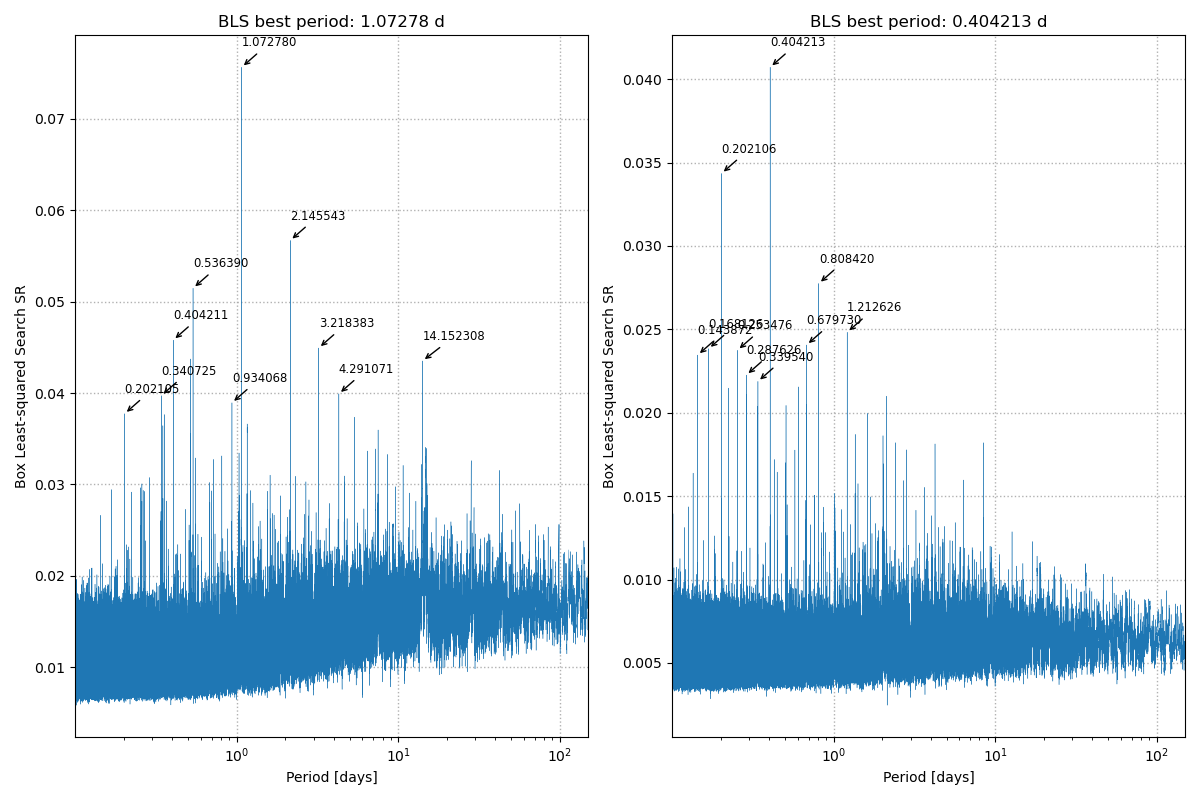
Figure 8: A periodogram of Gaia dr3 source ID 2216420454386370176 showing the lspvals as a function of orbital period. Left: The periodogram power values for period A. Right: The periodgram power values for period B after removing the signal of period A.

where max periodpower is the BLS-periodogram peak associated with the best period, $\overline{\mathrm{periodpower}}$ is the mean of powers and $\sigma_{\mathrm{periodpower}}$ is the standard deviation. In Astrobase these periodpowers are referred to as lspvals (Bhatti et al., 2017). For readers not familiar with the BLS algorithm, an example of a periodogram is shown in the appendix in Fig. 8. Here we see the periodogram power value of each orbital period. Additionally, Astrobase offers a function to calculate the signal-to-noise ratio (S/N) for each periodic signal (Bhatti et al., 2017). From the test sample we empirically determined that a RPH ¿ 10 and S/N ¿ 10 may indicate the presence of a double eclipsing binary. As it was not feasible to visually inspect all objects in the sample, we selected only candidates with RPH ¿ 10 and S/N ¿ 10. This significantly reduced the number of light curves that needed visual inspection to identify double eclipsing binary candidates. These selection criteria are discussed further in Sect. 6.

Some objects were, based on a high relative peak height and S/N, initially identified as quadruple candidate but appeared to exhibit a sinusoidal rather than an eclipsing signal. These objects were associated with relatively short periods $\mathrm{P_{B}}<0.30$ days, which could be an indication of a variable star in the binary system that lies on the instability strip, such as $\delta$ Scuti stars (Pietrukowicz et al., 2020). Another common false positive is associated with the imperfect removal of signal A. This would result in in period B being the same as period A, or an integer multiple of period A. We therefore removed any candidate for which period B was a multiple of period A.

When testing the method, it appeared that light curves containing high cadence observations (nights with more than 30 epochs) had a negative impact on the ability to find the right periods. This is probably caused by correlated noise introduced by the calibration of the data. Therefore, observations with more than 30 epochs per night were removed. A similar effect was observed by outliers in high and low flux. For this reason, outliers in normalised flux were removed using the interquartile range with a cut-off value of 5. Other unreliable data, flagged by the ZTF data process pipeline, was also removed. After this data pre-processing and cleaning, a minimum threshold of 500 data points per light curve was set for analysis. This decreased the sample size from 1 210 001 to 575 526 objects.

Based on the objects in the test sample, we set the period search range for new objects between 0.1 and 150 days with a stepsize determined by the minimum transit duration and observational period. We chose this lower limit as it is not expected to find any objects with shorter orbital periods (Drake et al., 2014). The upper limit was based on the five-year observational period of the ZTF and the decreasing likelihood of finding longer periods. For the transit duration, the BLS performed a search for a periodic signal lasting between 0.01 and 0.2 in phase.

Finally, we applied the pipeline to the 575 526 ZTF light curves. We used the HELIOS computer cluster to process the light curves. The average processing time per object is approximately 10 seconds.

We used the BLS output statistics to selected 5350 promising candidates. These were visually inspected in order to confirm the double eclipsing nature of the objects. At this point, we also determined, to the best of our abilities, what the two orbital periods are, since the BLS algorithm typically finds half the orbital period. Finally, we also checked if the photocenter position was correlated with the eclipse periods to identify chance alignments of two unrelated eclipsing binaries. The typical RMS positional accuracy is $\approx 0.1\arcsec$. No chance alignments were found in this manner.

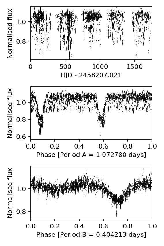
Figure 1: ZTF light curves of Gaia dr3 source ID 2216420454386370176. Upper panel: Normalised flux as a function of time. It shows two sets of eclipses with $\mathrm{P_{A}}=1.072780$ days and $\mathrm{P_{B}}=0.404213$ days. Middle panel: Phase folded light curve for binary A with $\mathrm{P_{A}}=1.072780$ days. We also see that not all data points fall nicely on the curve, indicating the presence of another signal. Lower panel: Phase folded light curve for binary B, after removal of the signal at period A, with $\mathrm{P_{B}}=0.404213$ days.

5 Results

Of the 575 526 light curves analysed (500 data points or more), 203 ($\approx$ 0.035$\%$) are identified as double-eclipsing binaries candidates. They are summarised in the appendix in Table 1, and an example is shown in Fig. 1. Almost all candidates for double eclipsing binaries are not currently known in any scientific literature (i.e. they are not listed as such on SIMBAD; Wenger et al., 2000). Only four of these 203 objects have been found in prior research and marked in Table 1 by an asterisk. One of these four objects, Gaia dr3 source ID 2003428628134264448, has previously been identified as a triple star system (TIC 388459317; Borkovits et al., 2021) but the ZTF data suggests that it is a double-eclipsing binary. The other three objects, Gaia dr3 source ID’s 2060949991271681664 (Zasche et al., 2022a), 407849617690288128 (TIC 354314226; Kostov et al., 2022b) and 158123726424621824 (TIC 150055835; Kostov et al., 2022b) have been identified as double eclipsing binary systems by previous studies that used TESS data. Using the ZTF data, we find that the periods of these objects agree between both studies.

The periods of the double eclipsing binaries in the ZTF sample range from 0.11 days to 323.20 days and the mean of periods A and B are 1.21 days and 10.52 days respectively, see Fig. 2. The figure shows that most objects have both periods shorter than a few days. Using a kernel density estimate, this distribution seems to be the same for the candidates and the test objects.

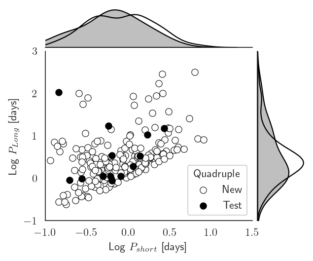
Figure 2: Periods A and B of 13 test objects and 203 quadruple candidates. Here $P_{short}$ is defined as the shortest period of A and B and $P_{long}$ as the longest period of A and B. The figure shows that most objects have both periods shorter than a few days. Using a kernel density estimate, this distribution seems to be the same for the candidates and test objects.

To understand if there is any bias in our search, all 1 210 001 binaries in the sample were plotted in an HR-diagram, see the left panel of Fig. 3. Here we see that the double eclipsing binaries, plotted separately as dots, are scattered throughout the diagram and do not seem to have any preferred location.

Since it is interesting to not only compare the double eclipsing binaries to the input sample but also to a general star population within the Milky Way, we refer to the HR-diagram of all stars in the Gaia dr3 archive within 200 pc of the sun. This can be seen in the right panel of Fig. 3. The quadruple candidates and test objects are systematically above the single stars in this diagram and are mostly Sun-like stars. We note, however, that quadruple systems on the HR-diagram have a lower magnitude of $2.5\log_{10}(4)=1.505$ compared to single stars, assuming all stars in the quadruple are similar and equally bright.

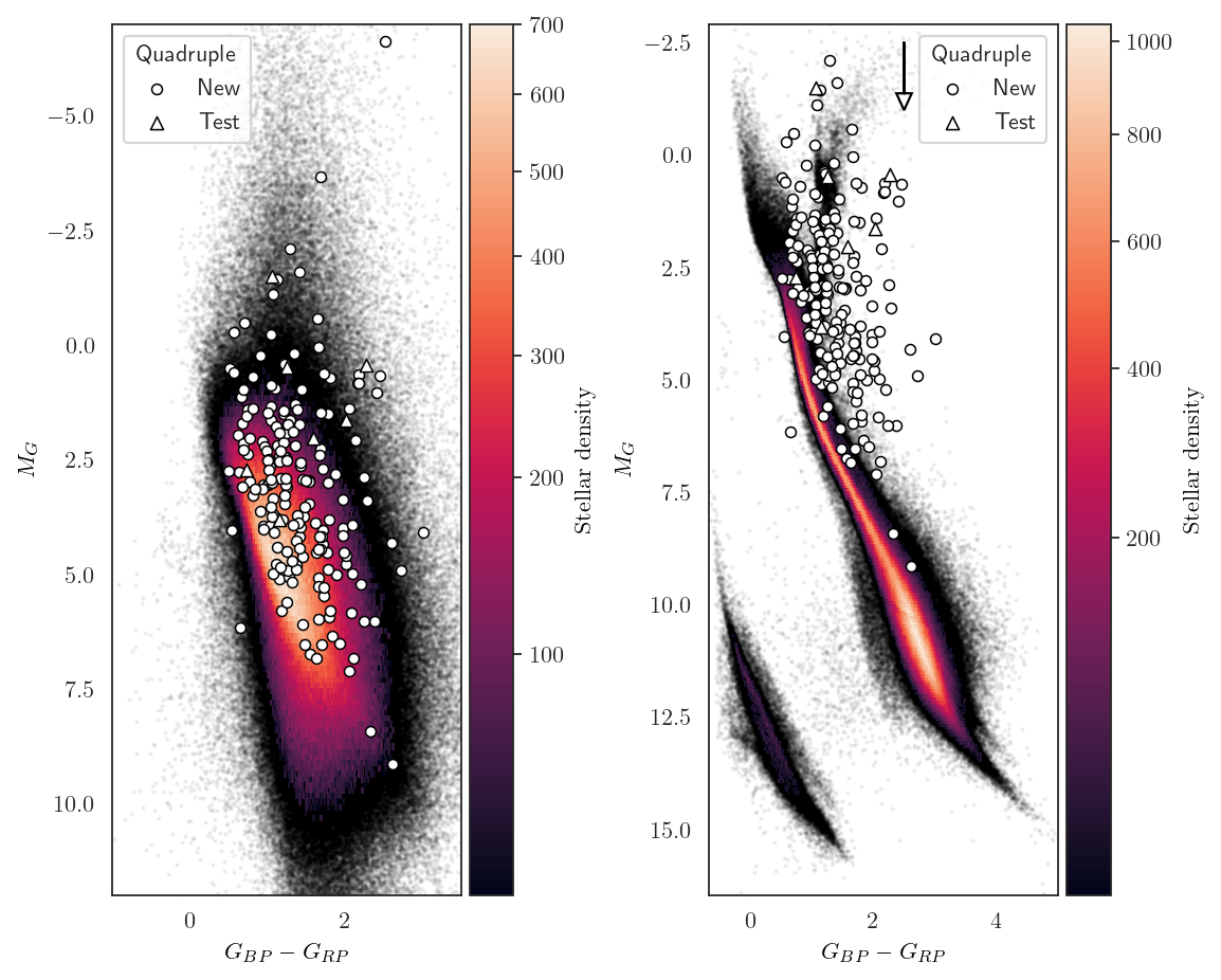
Figure 3: Left: HR-diagram of all 1 210 001 binary objects in the sample. The double eclipsing binary candidates and test objects, separately plotted as dots, are scattered throughout the diagram and do not seem to have any preferred location. Using the sun as a reference with $M_{G}=5$ and $G_{BP}-G_{RP}=1$, a larger number of objects seem to be similar to the sun. Right: An HR-diagram of all stars in the Gaia dr3 archive within 200 pc of the Sun. The candidates and test objects are systematically above the single stars in this diagram and are mostly sun-like stars. The arrow with a length of 1.505 magnitude indicates where one star in the quadruple system would lie, assuming all stars in the system are equally bright.

6 Discussion

6.1 Confusion with triple eclipsing systems

As we already noted; Gaia dr3 source ID 2003428628134264448 was previously identified as a triply eclipsing triple system (Borkovits et al., 2021) (a multistar system where all three stars eclipse each other). We initially identified this system as a quadruple because we detected a primary and secondary eclipse at a period of 88.8 days. However, as is shown by Borkovits et al. (2021) using well-sampled TESS and ground-based follow-up light curves; the eclipse shapes are complex and only consistent with a tertiary star that eclipses, and is being eclipsed, by a short period binary. Triple eclipsing stars are also extremely interesting for reasons similar to those of quadruple systems. For recent work on triple eclipsing systems, see Carter et al. (2011); Derekas et al. (2011); Hajdu et al. (2017); Mitnyan et al. (2020); Borkovits et al. (2021); Powell et al. (2022); Rappaport et al. (2022, 2023); Czavalinga et al. (2023)

The fact that one of our double eclipsing binary candidates turned out to be a triply eclipsing triple system, prompted us to reconsider the long period systems that we recovered. We focus on long period systems since, for triple systems, the outer orbit has to be at least 5 times the inner orbit, while a factor of 10 is required for slightly eccentric orbits (Mardling & Aarseth, 2001; Borkovits et al., 2021). With just the ZTF data, individual eclipses are not well-resolved, which makes an unambiguous identification of triples difficult. However, an eclipse of a triple eclipsing system is more noisy in a folded light curve because of the complex and changing shape of individual eclipses. We use this to determine whether some systems might be triple-eclipsing systems instead of double-eclipsing binaries.

Objects 2020970648976206208, 2210495392378660864, and 2038100043701450112 show somewhat irregular, long-duration eclipses in ZTF data and could be eclipsing triple systems. Objects 2058085351143518464, 2003428628134264448, 2201723866572302976, and 413930359370384384 show a primary and a shallow secondary eclipse at period B, with the primary eclipse somewhat irregular, suggesting that they could also be triply eclipsing systems. Object 2041659197183314304 shows well-behaved eclipses, and we judge that this system is unlikely to be a triply eclipsing system.

Objects 207943285475761280 and 2032118077650924672 are two systems for which the eclipse of the long period signal is much deeper in $g$ than $r$ and maybe a shallow secondary eclipse can be seen. This suggests that a large, cold star is eclipsed by a smaller, hotter star. We suspect that these are double eclipsing systems where one of the components has evolved off the main-sequence. For 260945106052343296 and 2012994482376100736 the period is too uncertain to draw any conclusions.

Since we cannot definitively classify these objects as triple eclipsing systems, we consider all these objects double eclipsing binary candidates in the rest of this paper. Follow-up light curve observations of the eclipses are needed for each object to definitively determine their nature.

6.2 Orbital period distribution

In general, binaries with shorter periods seem easier to detect than binaries with longer periods. One explanation is that stars in binaries with longer orbital periods are further apart from each other. As the orbital distance increases, the eclipse probability

$$\text{Eclipse probability}=\frac{R_{1}+R_{2}}{a}\propto P^{-2/3}$$ (2)

decreases since this requires a more precise alignment with the observer for the eclipse to be detected. In addition, longer orbital periods thus lead to shorter eclipse durations as fraction of the orbit. Some light curves showed that the eclipse duration of binary B was either very short (¡ 0.01 in phase), or contained very few data points, which makes it difficult for the algorithm to identify the eclipse. This agrees with the results shown in Fig. 2, where most double eclipsing binary candidates have both periods shorter than a few days.

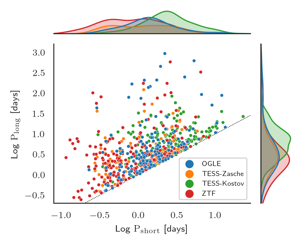
Figure 4: The orbital periods of double eclipsing binaries of the three largest samples: the sample from OGLE (Zasche et al., 2019), the sample from TESS by Kostov et al. (2022b, a) and Zasche et al. (2022b) and the ZTF sample from this work. Here $P_{short}$ is defined as the shortest period of A and B and $P_{long}$ as the longest period of A and B

The orbital periods of the candidates found in this research seem fairly similar to those found by Kostov et al. (2022a); Zasche et al. (2022b), see Fig. 4. However, one difference is that we find some shorter periods in this research. Whereas previous research shows that most objects show a period ratio of $\mathrm{P_{B}}/\mathrm{P_{A}}$ between 1 and 2 (Kostov et al., 2022a), in Fig. 5 we see that here also much smaller ratios are found, indicating a larger difference between period A and period B. An explanation for this can be the data cadence of TESS which is 26 days, meaning it most likely does not find any significant periods larger than approximately 13 days. Furthermore, short 30 minute exposures by TESS may lead to the spreading out of short eclipses, which is why TESS might not find very short periods either. We also note that all stars in our sample are listed in the Gaia catalogue. Any bias of Gaia towards shorter periods may therefore reflect in our results.

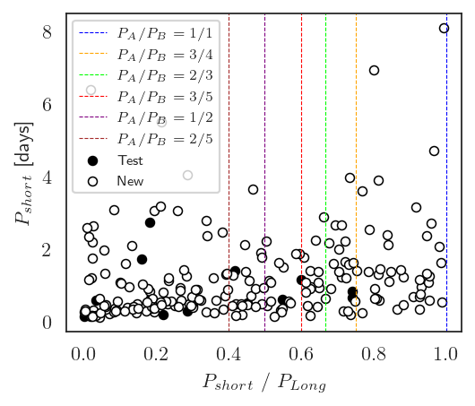
Figure 5: Period ratios $\mathrm{P_{short}}/\mathrm{P_{long}}$ of each object. Here $P_{short}$ is defined as the shortest period of A and B and $P_{long}$ as the longest period of A and B. The vertical lines indicate where potential harmonics would fall. We note that integer multiple harmonics were removed in the object search. However, non integer harmonics were not removed. Here we see that most objects do not fall on any of the harmonics lines indicating that there does not seem to be any particular correlation between the periods.

6.3 Detection efficiency and completeness

In this section, we briefly discuss the detection efficiency and completeness of our search. Of the 575 526 analysed objects, at least 203 ($\approx$ 0.035%) passed the visual inspection tests and showed to be a double eclipsing binary candidate rather than a binary system. This is approximately a factor 4.5 lower success rate than Zasche et al. (2022b) (116 out of 70.000) and a factor 7 lower than Pawlak et al. (2013) (15 out of 6138). However, we note that OGLE-III has observed all stars in a dense area in the Small Magellanic Cloud for a longer period of time (Pawlak et al., 2013). Zasche et al. (2022b) have, like this research, only looked at eclipsing binaries, but a difference with this research is the data cadence, which for ZTF typically is one observation per night only for five years. TESS, on the other hand, provides continuous undisturbed photometry for 26 days (Zasche et al., 2022b). Lastly, the angular resolution of ZTF, OGLE, and TESS are very different. This, combined with the new method used here, makes it difficult to compare success rates, but could explain the difference.

In the rest of this section, we briefly discuss a few causes that limit the completeness of our search. First, we consider the efficiency of our quadruple detection method. Our method was able to retrieve the correct periods for most known objects in the test dataset. For periods that could not be recovered, further investigation revealed why this was not possible. In some cases, many data points were flagged as unreliable, leaving only very few data points in the light curve for period finding. In other instances, the eclipse depth of one binary was very small, on the order of a few percent, making it difficult for the algorithm to detect any periodic signal. Other reasons why the algorithm was not successful included that some light curves showed a very small trend in flux over time, resulting in the cadence of the telescope being found as significant period; this typically being one or two days. Even light from the Moon coming in as background noise could lead to the period of the Moon being found to be a significant period. For compact double eclipsing binaries, eclipse-timing variations (ETV) can smear periodic signals which may affect the period finding. However, when comparing our results with known systems with ETV, we found this not to be the case. We therefore expect this method to be suitable for finding compact double eclipsing binaries.

The completeness of our search for double eclipsing binaries is also limited by our use of the Gaia eclipsing binary catalogue. When we look at the results of other studies (Kostov et al., 2022a, b; Zasche et al., 2022b), we see that approximately 30% of the found quadruples are in the Gaia catalogue. In this research we have only looked at ZTF objects that are known in the Gaia catalogue. This means that potentially three times more quadruples can be found in the ZTF data that are not in the Gaia catalogue.

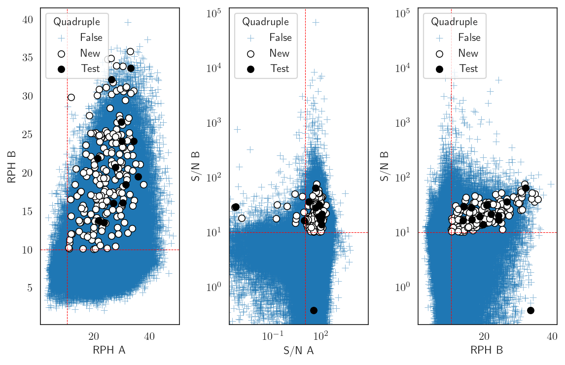
Figure 9: The relative peak height and S/N of all objects including double eclipsing binary candidates and test objects. Left: Relative peak heights A and B for all objects. Middle: S/N A and S/N B results for all objects. Right: S/N B and relative peak height B of all objects. We see that quadruples can have a wide range of RPH and S/N values. However, this also means that more can be found at values of RPH ¡ 10 & S/N ¡10.

As it was not practical to look at 575 526 light curves, we used automatically calculated statistics to significantly decrease the number of light curves to inspect which could also affect the completeness of our search of the ZTF data. We used the test objects to empirically determine cuts; relative peak height $>10$ and S/N $>10$. As can be seen in Fig. 9, the wide range of values of relative peak height and S/N cannot reliably indicate whether an object might be a quadruple candidate. This suggests that more double eclipsing binaries can be found for values of relative peak height and S/N below 10. It can also be seen in the figure that some objects did have a high relative peak height and S/N but were not identified as a quadruple candidate. This could have several reasons. In some cases, the algorithm was not able to completely remove the first periodic signal, which means that the signal, or an harmonic, was returned again for period B. Other explanations include, but are not limited to, an outlier in the light curve, the cadence of the telescope, or the influence of the Moon. Sometimes the algorithm did not find an eclipsing signal but a sinusoidal signal, possibly due to the pulsation of one of the stars in the eclipsing binary. Even though this is not a double eclipsing binary, a strong periodic signal was still found, resulting in a high relative peak height and S/N.

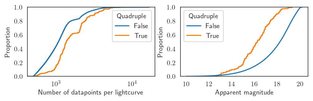
Figure 6: Left: Cumulative histogram for the number of data points per light curve. After passing a threshold of approximately 1000 data points there is a significant increase in the quadruple detection efficiency. Note that the plateau and discontinuity at around 2000 data points is a result of the ZTF survey strategy. Right: Cumulative histogram for the magnitude of stars for the complete sample and quadruple candidates in the magnitude range 13-20.5. We see that for stars fainter than $G\gtrsim 18$ the quadruple detection efficiency rapidly approaches zero. The sharp increase at $G\approx 15$ is not fully understood.

We suspected that the detection efficiency of double eclipsing binary stars is also strongly affected by the number of epochs in the light curve. If we look at the left panel in Fig. 6 we see a cumulative histogram for the number of data points per light curve. It shows that, only after passing a threshold of approximately 1000 data points, the quadruple detection efficiency significantly increases. After that, there are more double eclipsing binaries as the number of data points increases. The difference, however, is small. This means that, as ZTF keeps collecting data (or ZTF is combined with external data), we can expect the number of detectable double eclipsing binaries to double.

We also briefly consider to what brightness we can reliably find double eclipsing binaries in ZTF data. On the right panel in Fig. 6 we see a cumulative histogram for the magnitude of stars, both for the complete sample and for the quadruple candidates. The ZTF has looked at stars in the magnitude range 13-20.5. Since the curve of the quadruples is constantly above the overall sample curve, this indicates that it is easier to find quadruples for bright stars compared to faint stars. Almost all quadruples have a magnitude of $G\lesssim 18$, while only half of the input sample is fainter than this limit. We conclude that the light curve signal-to-noise ratio is too low for sources fainter than $G\approx 18$. As can be seen in Masci et al. (2019), the RMS precision is $\approx 1\%$ for sources brighter than 18 magnitude, but the precision degrades rapidly for fainter sources.

To summarise, we expect that future research can find at least three to four times more quadruples by including the following considerations. First, the search should be not limited to the Gaia eclipsing binary catalogue but the entire ZTF database can be searched instead. Secondly, systems with a relative peak height and S/N lower than 10 should also be considered. Thirdly, longer observation time of the ZTF will lead to more data points which has a positive effect on quadruple finding. Lastly, by using an automatic detection method that can replace visual detection, for instance machine learning, all the light curves can be analysed more efficiently.

7 Conclusions and future work

We have developed a method to systematically search for double eclipsing binaries in sparsely sampled data. Using this method we found 198 new double eclipsing binaries candidates in the ZTF data. The periods of the objects ranged from 0.11 days to 323 days with a mean of periods A and B of 1.21 days and 10.52 days respectively. By searching the entire ZTF database, increasing the number of data points per light curve, and implementing an automatic detection mechanism that replaces visual inspection, we expect that at least three to four times more quadruples can be found using this method. Other recommendations for future work are; to apply this method to data collected by other telescopes such as Gaia. In addition, we recommend that the multi star systems are included in the target lists of large multiplex spectroscopic surveys such as SDSS, DESI, and WEAVE in order to obtain phase-resolved spectra of the quadruple candidates to further investigate their properties. Lastly, detection of eclipse-timing variations in the double eclipsing binaries can definitively prove their quadruple nature.

Appendix A Additional figures

For the ZTF, the periods of objects that lie in the Galactic plane can be more easily retrieved. This is can also be seen in Fig. 7 where the location of all quadruple candidates and test objects are plotted. These results agree with the results found in earlier research (Zasche et al. 2022b; Kostov et al. 2022a). It is most likely that the number of double eclipsing binaries is higher in the Galactic plane as a result of higher star density.

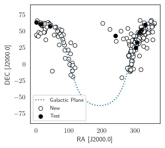
Figure 7: Right ascension (RA) and declination (DEC) of the double eclipsing binary candidates and test objects in this research. As expected, most candidates lie in the Galactic plane. No objects are seen below a declination of -30° as this is not visible by the ZTF.

Appendix B Summary of double eclipsing binary candidates

Table 1 in this appendix lists all new double eclipsing binaries we found in ZTF.

Table 1: Summary of the double eclipsing binary candidates. For each candidate the location (RA & DEC), Gaia dr3 source ID, periods ($\mathrm{P_{A}[d]}$ & $\mathrm{P_{B}[d]}$) and eclipse depths ($\mathrm{D_{A}}$ & $\mathrm{D_{B}}$) are given. Four objects have been found in previous research and are marked here with an asterisk. The object marked with a ”T” was initially identified as a quadruple, but further investigation revealed that this is, in fact, a triple system.

RA [J2000.0]	DEC [J2000.0]	Gaia dr3 source ID	$\mathrm{P_{A}[d]}$	$\mathrm{D_{A}}$	$\mathrm{P_{B}[d]}$	$\mathrm{D_{B}}$
1.461502	44.447714	386474080852740992	2.599973	0.178	0.114405	0.017
2.702797	43.426465	384686137507666944	0.561156	0.057	0.30431	0.02
3.255083	66.065778	528173641885393792	1.377078	0.007	1.958498	0.067
5.530266	63.915121	431071367690614016	1.993434	0.207	2.83458	0.12
6.850741	42.275447	382118159381427840	0.302332	0.045	11.331499	0.063
8.806599	48.41824	390942874067575936	0.254808	0.066	100.03476	0.159
13.007138	60.631402	427296611137250432	1.39752	0.108	1.233086	0.034
13.938753	62.946494	523702890174595456	0.620434	0.129	0.766964	0.071
14.457916	46.742013	377967807928167552	1.557556	0.059	0.569134	0.181
17.516555	60.901287	522445255030705920	0.357662	0.183	0.653228	0.098
18.801672	57.606248	413446544200880896	0.951178	0.076	7.547427	0.073
20.433859	58.575703	413930359370384384	1.745764	0.211	74.595949	0.184
23.839866	48.216903	399464707656254976	6.934429	0.026	8.655612	0.066
24.594285	62.368258	511572184543165184	1.111992	0.017	0.893415	0.099
25.46978	48.453185	405343761970536320	3.214925	0.181	0.475366	0.051
26.105725	57.363963	505854376178706048	0.395542	0.283	0.613647	0.075
26.99833	58.484187	506382008620308352	0.469946	0.117	1.607418	0.082
27.345582	51.957608	407610302112852992	0.27613	0.067	4.742124	0.105
27.478311	61.054208	511202954794627072	2.522958	0.088	2.118876	0.037
27.619643	53.266914	407849617690288128∗	1.388514	0.182	1.842243	0.133
29.369827	36.938288	330442487264141952	2.165996	0.148	3.201325	0.069
32.660282	56.361212	457045959812411520	2.907525	0.249	1.766785	0.083
35.274278	59.921344	507367789513371392	4.733592	0.119	1.111969	0.06
35.979435	63.411351	514335841379134336	1.718536	0.264	1.220503	0.075
36.881203	63.214977	514291963992396928	3.006382	0.093	0.212537	0.019
38.031578	62.343023	513987498047116544	1.019208	0.086	0.948252	0.071
38.292867	59.484742	465028723463664384	3.460204	0.192	0.92533	0.045
39.195205	60.984813	465274395594682240	3.887904	0.148	1.896361	0.083
42.417307	58.265701	461012963401936256	1.060832	0.048	10.593118	0.034
44.301404	59.454303	461553472144934656	0.270063	0.053	1.385304	0.049
49.178341	-10.308834	5166225811703486464	0.275808	0.248	2.432133	0.098
54.711333	44.047482	244408588611828096	0.178865	0.145	0.243028	0.022
57.458651	56.117922	445534966419218560	1.292364	0.246	1.088451	0.051
59.624908	56.534336	469545650369412864	0.224785	0.178	1.551227	0.05
64.168902	50.317876	271381051952218496	2.245528	0.108	1.40276	0.05
67.213782	42.115243	228205115816360832	1.125492	0.13	2.201828	0.02
67.217417	48.572915	258090121033397248	5.48996	0.156	25.643685	0.035
68.629624	48.698441	257683439171736576	0.81849	0.107	4.499209	0.08
69.925315	29.134575	158123726424621824∗	1.58676	0.128	13.783777	0.06
72.308262	52.265466	260945106052343296	3.070683	0.241	37.120622	0.061
73.106774	45.534572	206454920393197440	0.583875	0.365	0.715742	0.089
76.053644	42.807356	202201601392851072	0.624014	0.05	14.132366	0.087
77.972018	51.672042	262779881722935424	1.637614	0.193	2.266959	0.101
80.461508	37.37017	184468231186516352	2.345842	0.133	6.86879	0.09
80.679986	37.664808	184497570107735296	2.3771	0.094	2.839768	0.055
82.738969	44.803406	207943285475761280	52.829036	0.274	1.184305	0.066
83.858615	33.004921	3448886540015107584	2.989964	0.115	0.52143	0.06
86.591414	28.923839	3443402279093860096	0.53534	0.144	0.541528	0.079
87.5282	21.330875	3400120484904001408	3.572446	0.166	1.759766	0.066
88.00886	8.805691	3335190578070549632	0.36877	0.083	1.890454	0.068
96.842245	21.72127	3376140681762631168	0.39992	0.093	0.842531	0.049
98.587002	7.745466	3325963098535865728	0.584642	0.307	0.6136	0.053

Table 2: Continued

RA [J2000.0]	DEC [J2000.0]	Gaia dr3 source ID	$\mathrm{P_{A}[d]}$	$\mathrm{D_{A}}$	$\mathrm{P_{B}[d]}$	$\mathrm{D_{B}}$
101.872246	-0.444575	3113400013097881600	0.86539	0.121	2.182992	0.048
103.057739	-1.125556	3112366227355971328	0.948312	0.155	0.632336	0.069
104.069404	15.809035	3355042672829484032	2.502663	0.177	0.530042	0.06
105.184549	32.479562	890716293806690816	0.263998	0.105	3.144128	0.136
105.242128	-16.522209	2935716391431248256	0.424388	0.076	7.412474	0.067
109.571295	1.765508	3111928351141425792	0.274758	0.174	0.144463	0.054
109.612639	-10.149447	3047190824491991168	0.45911	0.163	0.25037	0.05
111.089388	-2.032067	3061770932787038336	0.422212	0.082	0.966995	0.054
111.47435	-19.281677	2930398740886024064	0.347152	0.219	2.294894	0.144
117.697495	28.467895	875709132614498560	0.442358	0.158	1.466414	0.069
118.096034	-5.697484	3044312990239139968	1.452632	0.176	1.779009	0.072
202.102553	61.876817	1663741485747221248	2.770754	0.15	8.163296	0.08
223.42518	52.715832	1594082407606370176	2.700472	0.074	1.488501	0.043
242.649013	34.62108	1323756753679794048	7.041158	0.114	0.128904	0.014
257.277242	49.948796	1414515322519168640	0.301544	0.197	0.231617	0.019
259.250732	-20.297582	4115999620890627968	0.621141	0.24	0.773402	0.114
263.775976	38.311866	1343353448205456256	3.048348	0.095	11.792556	0.033
273.743299	39.207529	2109307852667550464	2.205617	0.187	4.373204	0.029
276.008132	-5.774128	4161007815803011968	3.070536	0.211	1.371504	0.102
278.026086	54.402996	2147458221793949184	3.109478	0.097	1.853905	0.079
279.117985	-8.525243	4156431820198005376	1.407928	0.281	1.331908	0.085
279.719282	13.163625	4508288602094506112	0.399492	0.061	1.528379	0.102
280.635591	-5.252461	4256607950976483968	1.907376	0.222	0.903688	0.036
280.635808	13.120684	4505600296166989312	4.870614	0.097	4.70215	0.019
280.713417	34.65467	2091761983553949696	0.271486	0.204	0.372731	0.028
281.121588	11.13593	4504043245957168640	10.015578	0.077	1.042907	0.022
282.145741	30.399305	2041659197183314304	0.283664	0.061	55.568657	0.06
282.312661	13.469479	4505497904155844992	0.28221	0.303	3.150768	0.103
283.996449	28.282368	2040256804464235648	5.739774	0.104	0.139815	0.012
284.492451	-11.193995	4201927347951103488	0.513114	0.405	0.453093	0.05
285.268359	18.064422	4517289341731165568	1.056042	0.07	0.545708	0.031
286.391765	16.558561	4513882917294832384	0.875846	0.043	2.838248	0.022
286.904493	-9.457319	4204113619406564480	0.33327	0.097	0.867417	0.047
287.114664	-8.543055	4204326997705570304	0.272314	0.3	0.170204	0.061
287.445354	19.597742	4516377056329377664	1.035768	0.171	6.325886	0.082
287.648865	16.355321	4513263857861420672	0.45636	0.166	2.129335	0.1
287.884621	46.028573	2130268255146656128	0.422266	0.269	1.029215	0.035
288.026347	23.298684	4521240642906912128	3.00593	0.011	1.616295	0.071
288.248394	0.080909	4264206469687918848	3.166976	0.208	1.852653	0.103
288.471817	-1.094539	4263034768239285632	1.862082	0.16	0.592354	0.053
288.648651	22.157332	4520164564651728128	0.355088	0.09	0.32902	0.045
288.825262	4.312846	4293109022582320640	0.390062	0.277	0.164066	0.11
289.517888	15.160579	4320727174167431296	2.163692	0.033	1.607176	0.042
290.184501	28.541396	2038100043701450112	0.325552	0.122	79.87107	0.122
290.604938	9.66816	4308597705466532224	5.097978	0.173	1.412602	0.057
290.991691	35.958626	2050141310916611584	3.877374	0.021	4.766349	0.047
291.640789	4.331223	4292639977810529152	1.64215	0.063	1.061804	0.058
291.714347	18.228635	4323257219102940288	1.588804	0.186	2.302579	0.077
291.820676	35.97582	2049954600104034432	4.030792	0.113	14.062535	0.062
293.462031	19.846805	1825483906846429056	6.45557	0.145	2.467705	0.047
293.504188	27.432478	2025279046615280512	2.759184	0.134	0.863998	0.026
293.592507	11.006839	4314657904341880960	3.349092	0.109	1.32064	0.027
293.657387	19.881442	1825578567909317760	4.770348	0.152	2.118271	0.038
293.823697	25.752582	2021549301357843328	0.417266	0.168	0.182446	0.089

Table 3: Continued

RA [J2000.0]	DEC [J2000.0]	Gaia dr3 source ID	$\mathrm{P_{A}[d]}$	$\mathrm{D_{A}}$	$\mathrm{P_{B}[d]}$	$\mathrm{D_{B}}$
294.156333	14.316215	4318042922678224768	1.840298	0.023	0.915486	0.087
294.332664	27.158424	2025146250574308480	0.430934	0.184	0.698726	0.062
294.518815	-7.404433	4207090654517833344	3.426032	0.186	0.315937	0.04
294.832597	26.871716	2025081478136260480	3.072568	0.066	2.212912	0.052
294.839444	35.975154	2048268017993738624	0.234828	0.043	4.944031	0.052
294.933937	20.202009	1825745006505362048	7.807304	0.051	3.649778	0.042
295.309706	42.822037	2077913565886105344	0.373692	0.344	0.322663	0.03
295.479516	34.635703	2047323949824485376	2.346872	0.18	2.481432	0.055
295.527859	22.054362	1827708802964917888	0.545902	0.187	0.96728	0.047
295.87929	25.881643	2021774220180193536	1.357318	0.0	2.09345	0.026
296.235173	29.583425	2031977619399032448	8.147016	0.064	8.083514	0.023
296.585034	23.395937	2020056405032433152	0.812118	0.18	0.753871	0.086
296.895517	25.636448	2020970648976206208	6.375142	0.168	323.201568	0.109
296.955946	30.241753	2032118077650924672	171.076078	0.28	2.335024	0.089
297.00612	24.058537	2020490437267187712	1.35866	0.148	1.729201	0.093
297.034812	30.08806	2031925182082532608	3.590404	0.001	0.789163	0.032
297.056926	25.787105	2026976864358731904	1.425158	0.0	0.89166	0.105
298.002327	31.866931	2033828574151981184	1.768354	0.231	0.571495	0.122
298.172845	26.864218	2027154955201119488	1.647592	0.093	1.191313	0.026
298.530047	24.682368	1834469768675202560	2.881026	0.081	4.353022	0.036
298.820248	32.01454	2033656156987971840	7.548416	0.327	0.159107	0.049
298.881534	29.89156	2030312580776346240	0.462184	0.179	7.651529	0.06
298.908525	32.746538	2034277144881784704	2.452324	0.245	0.558699	0.026
299.522067	30.246542	2030426861313716224	1.305256	0.061	1.607371	0.019
299.620393	33.527522	2034419218049672704	1.411226	0.099	1.614413	0.072
299.976835	29.83971	2030212490900354176	1.189566	0.022	3.314311	0.025
301.355473	34.989363	2058617549147113728	2.08353	0.045	15.704131	0.051
301.37899	35.97206	2059117002318116096	1.741608	0.114	1.064947	0.033
301.391172	42.318524	2074882590295669376	1.127028	0.197	2.46579	0.132
302.250175	21.436492	1829670778385777920	5.414028	0.109	3.970943	0.085
302.637062	38.400325	2061735248734886400	1.079346	0.226	0.468297	0.029
302.98334	36.463072	2059178162649303808	5.993378	0.266	0.563785	0.056
303.229266	27.908953	1836995514370597120	0.374674	0.076	3.126105	0.05
303.523133	38.382872	2060949991271681664∗	1.144666	0.129	0.481849	0.017
304.151811	41.930677	2068658632915468672	4.363316	0.078	1.242846	0.052
304.756649	37.920034	2061050802729418496	1.325726	0.172	0.813421	0.097
304.795015	30.560399	1861612037845705728	5.302642	0.194	0.323736	0.037
306.408352	37.894974	2058085351143518464	1.152476	0.193	85.498447	0.139
308.681181	48.20847	2167733048719069312	2.17693	0.17	0.584749	0.086
308.779214	35.826622	2056704914305732096	5.152764	0.146	0.910183	0.069
309.435623	30.852742	1862347439319475072	0.920364	0.145	1.417808	0.094
311.55134	31.682545	1859824197571796736	0.283018	0.133	0.394832	0.064
311.97923	34.771038	1869489385821202816	0.488582	0.115	2.110629	0.109
312.564502	12.412033	1760943570684334208	3.047312	0.209	15.580245	0.076
312.603366	47.202077	2166511040319614208	0.38052	0.147	1.264149	0.127
313.727051	39.848684	1872913471188045184	2.26941	0.054	0.678956	0.023
314.203035	66.204173	2245787855903677952	1.313048	0.21	1.250967	0.228
315.998617	47.984506	2165439879783209344	3.822778	0.095	2.650119	0.037
316.499668	36.761395	1868409321799840768	0.543036	0.063	0.725643	0.036
316.935639	47.04712	2165141946503725056	1.272084	0.103	3.086064	0.035
317.167097	-8.177796	6897094092939104768	0.223992	0.027	0.622656	0.041
317.354427	55.485175	2176903937763785088	3.446506	0.256	3.158925	0.236
318.20909	56.26039	2177329891137899904	0.90333	0.253	0.515231	0.087
318.442107	51.071054	2166229226047556096	15.0598	0.169	3.180452	0.086

Table 4: Continued

RA [J2000.0]	DEC [J2000.0]	Gaia dr3 source ID	$\mathrm{P_{A}[d]}$	$\mathrm{D_{A}}$	$\mathrm{P_{B}[d]}$	$\mathrm{D_{B}}$
321.274386	49.322575	2170863908089217280	3.714414	0.154	2.643588	0.078
322.785455	37.809557	1952168090372267008	1.158128	0.035	1.25026	0.023
322.795044	41.61673	1967117802081173504	4.672324	0.102	3.584245	0.036
324.064461	40.289056	1966045232784781952	0.264192	0.119	0.779663	0.061
325.003123	56.109079	2178057359827382144	3.296832	0.225	1.291317	0.036
325.081161	48.44538	1978029359778790016	0.678389	0.01	0.746095	0.054
325.126003	39.737305	1953928099249228032	1.068532	0.22	1.123977	0.027
325.523023	58.222165	2178581380197081216	1.810504	0.115	0.707697	0.062
325.791627	27.217748	1800509737128120320	0.85369	0.239	3.215801	0.166
326.593483	49.781513	1978958103506727424	0.421342	0.068	1.667499	0.039
327.020592	62.78985	2216420454386370176	2.14556	0.228	0.404213	0.082
327.271647	58.943552	2202597664775578112	1.06056	0.143	2.05528	0.107
328.521806	57.784601	2199284050276697216	0.433052	0.121	1.459645	0.106
329.000459	52.050747	1981103972253289088	0.685961	0.114	0.739756	0.027
329.356711	45.001855	1973338392191011584	0.397442	0.112	6.522002	0.093
329.904956	43.718061	1961000256819235200	0.473181	0.095	0.964035	0.103
330.10459	57.341933	2199104211409698816	0.979846	0.194	0.443703	0.067
330.629145	55.984692	2198180415480756096	1.328192	0.0	22.393498	0.086
332.366702	56.166443	2197966251234148352	2.705704	0.168	2.822163	0.04
332.720979	59.64723	2199925099913441920	2.15344	0.175	1.57226	0.067
332.943294	54.42099	2005474711889658624	3.234134	0.101	0.617324	0.135
333.801196	53.749768	2004590532743751424	0.340078	0.058	2.522543	0.034
334.655366	55.538438	2005911802117955968	1.508362	0.197	0.947192	0.097
335.103223	36.014911	1905994992912248448	0.834723	0.19	0.422142	0.116
335.115083	24.563415	1878929101147587200	2.107929	0.256	2.068346	0.048
337.436575	54.279883	2001849763802035840	2.263908	0.235	0.545817	0.03
337.832153	60.857037	2201723866572302976	2.627162	0.107	101.237102	0.125
339.088072	47.538959	1986716807300365696	6.451769	0.218	0.164641	0.043
339.963254	54.98005	2003428628134264448∗T	2.184788	0.145	88.853882	0.143
340.921211	57.261299	2007240188275431936	1.625996	0.064	1.379002	0.038
341.302946	56.012542	2003907912126462592	0.404544	0.102	2.944626	0.058
341.422596	53.230019	2002122850696945664	3.484958	0.063	2.227952	0.036
342.74	58.714103	2007474143733297152	1.63917	0.116	1.617598	0.023
344.803515	48.306854	1984790600366568576	0.699564	0.452	1.513966	0.034
347.564145	65.090617	2208692193312331904	5.095412	0.059	1.198208	0.03
349.093506	66.228219	2210495392378660864	2.568998	0.241	285.579588	0.218
350.55902	56.248535	1997226175657082496	0.351738	0.091	1.855745	0.043
351.050509	59.819433	2010769070836151424	1.312382	0.17	0.89549	0.057
352.521122	57.484618	1998851258144250112	0.280512	0.094	1.619602	0.047
352.593979	48.961381	1942119756681849216	4.303021	0.4	0.149352	0.039
353.524226	36.870485	1918839728265382912	0.366704	0.208	4.201864	0.116
358.069196	62.459358	2012994482376100736	1.950456	0.256	34.404796	0.119
358.221987	61.525403	2012695312133566208	3.21884	0.179	2.533716	0.056