Revisiting Recommendation Loss Functions through Contrastive Learning (Technical Report)

Abstract

Inspired by the success of contrastive learning, we systematically examine recommendation losses, including listwise (softmax), pairwise (BPR), and pointwise (MSE and CCL) losses. In this endeavor, we introduce InfoNCE+, an optimized generalization of InfoNCE with balance coefficients, and highlight its performance advantages, particularly when aligned with our new decoupled contrastive loss, MINE+. We also leverage debiased InfoNCE to debias pointwise recommendation loss (CCL) as Debiased CCL. Interestingly, our analysis reveals that linear models like iALS and EASE are inherently debiased. Empirical results demonstrates the effectiveness of MINE+ and Debiased-CCL.

Introduction

Recommendation and personalization have become fundamental topics and applications in our daily lives (Aggarwal 2016; Zhang et al. 2019). Recent research has demonstrated the difficulty of properly evaluating recommendation models (Dacrema, Cremonesi, and Jannach 2019), even for the (simple) baselines  (Rendle, Zhang, and Koren 2019). A few latest studies have shown the surprising effectiveness of simple linear models and losses, such as iALS (Rendle et al. 2022, 2021) and SimpleX (CCL) (Mao et al. 2021). Concurrently, recommendation research is placing greater emphasis on the need for a deeper (theoretical) understanding of recommendation models and loss functions  (Jin et al. 2021a).

Drawing inspiration from recent studies, this paper delves deep into an analysis and comparison of loss functions, pivotal in developing recommendation models (Mao et al. 2021). In the past few years, contrastive learning (Chen et al. 2020; Oord, Li, and Vinyals 2018; Chuang et al. 2020) has shown great success in various learning tasks, such as computer vision and NLP, among others in both supervised and unsupervised settings. It aims to learn a low dimensional data representation so that similar data pairs stay close to each other while dissimilar ones are far apart. Notably, contrastive loss functions (such as InfoNCE)  (Chen et al. 2020; Oord, Li, and Vinyals 2018) share striking resemblances with recommendation loss functions, like BPR (Bayesian Personalized Ranking) and Softmax (Aggarwal 2016). The latter aims to align user embeddings more closely with the items they favor. The burgeoning (theoretical) exploration in contrastive learning presents an opportunity to deepen our understanding of recommendation losses and design new ones through the perspective of contrastive losses. Interestingly, recent studies (Zhou et al. 2021; Wang et al. 2022) have begun integrating contrastive learning approaches into individual recommendation models. Yet, a comprehensive comprehension of recommendation loss functions viewed through the prism of contrastive learning remains to be fully developed and explored.

Specifically, the following key research questions remain unanswered: How do listwise softmax loss and pairwise BPR (Rendle et al. 2009) (Bayesian Pairwise Ranking) loss relate to these recent contrastive losses (Chuang et al. 2020; Oord, Li, and Vinyals 2018; Belghazi et al. 2018)?Can we design better recommendation loss functions by taking advantage of latest contrastive losses, such as InfoNCE (Oord, Li, and Vinyals 2018), decoupled  (Yeh et al. 2022) and mutual information-based losses(Belghazi et al. 2018)? Can we debias $L1$ (mean-absolute-error, MAE) and $L2$ (mean-squared-error, MSE) loss function similar to debiasing contrastive loss, InfoNCE  (Chuang et al. 2020)? More specific, do the well-known linear models (based on $L2$ loss), such as iALS (Rendle et al. 2022; Hu, Koren, and Volinsky 2008a; Rendle et al. 2021) and EASE (Steck 2019), need to be debiased with respect to contrastive learning losses?

To answer all these questions, we made the following contributions in this paper:

• We revisit commonly used contrastive learning loss - InfoNCE in the recommender system and propose its general format - InfoNCE+ by introducing balance coefficients on the denominator as well as the positive term inside. Our empirical results appeal that the discarding of the positive term in the denominator would lead to superior performance which aligns with the latest decoupled contrastive loss  (Yeh et al. 2022). We further theoretically explore it through mutual information theory and simplify it as MINE+. Finally, through the lower bound analysis, we are able to relate the contrastive learning losses and BPR loss.

• By leveraging the latest debiased contrastive loss (Chuang et al. 2020), we propose debiased InfoNCE and generalize the debiased contrastive loss  (Chuang et al. 2020) to the pointwise loss CCL (Mao et al. 2021)) in recommendation models, referred as Debiased CCL. We then examine the well-known linear models with pointwise $L2$ loss, including iALS and EASE; rather surprisingly, our theoretical analysis reveals that both are inherently debiased under the reasonable assumption with respect to the contrastive learning losses.

• We experimentally validate the debiased InfoNCE and point-wise losses indeed perform better than the biased (commonly used) alternatives. We also show the surprising performance of the newly introduced mutual information-based recommendation loss and its refinement (MINE+).

To the best of our knowledge, this is the first study to systematically investigate the recommendation loss functions through the lens of contrastive learning. It not only helps better understand and unify the recommendation losses but also introduces new loss functions, such as MINE+ and Debiased CCL, which are inspired by contrastive learning and introduced to the recommendation realm for the first time. Moreover, we establish the unexpected debias properties of iALS and EASE, unveiling significant characteristics previously unexplored. These findings serve to construct a foundational (theoretical) scaffold for better understanding of recommendation losses.

Background

In this section, we briefly review the commonly-used recommendation loss function - BPR (Bayesian Personalized Ranking)  (Rendle et al. 2009), softmax  (Covington, Adams, and Sargin 2016; Zhou et al. 2021), and InfoNCE (Oord, Li, and Vinyals 2018).

Notation: We use $\mathcal{U}$ and $\mathcal{I}$ to denote the user and item sets, respectively. For an individual user $u\in\mathcal{U}$, we use $\mathcal{I}^{+}_{u}$ to denote the set of items that have been interacted (such as Clicked/Viewed or Purchased) by the user $u$, and $\mathcal{I}\backslash\operatorname*{\mathcal{I}}^{+}_{u}$ to represent the remaining set of items that have not been interacted by user $u$. Similarly, $\operatorname*{\mathcal{U}}^{+}_{i}$ consists of users interacting with item $i$, and $\operatorname*{\mathcal{U}}\backslash\operatorname*{\mathcal{U}}_{i}^{+}$ includes remaining users. Often, we denoted $r_{ui}=1$ if item $u$ is known to interact with of item $i$ and $r_{ui}=0$ if such interaction is unknown.

Given this, most of the recommendation systems utilize either matrix factorization (shallow encoder) or deep neural architecture to produce a latent user vector $v_{u}$ and a latent item vector $v_{i}$, then use their inner product ($<v_{u},v_{i}>$) or cosine ($<v_{u}/||v_{u}||,v_{i}/||v_{i}||>$) to produce a similarity measure $\hat{y}_{ui}$. The loss function is then used to produce a (differentiable) measure to quantify and encapsulate all such $\hat{y}_{ui}$.

BPR Loss: The well-known pairwise BPR loss is the most widely used loss function in the recommendation, which can be written as:

$$\begin{split}&{\mathcal{L}}_{bpr}=\operatorname*{\mathbb{E}}_{u}\operatorname*{\mathbb{E}}_{i\sim p_{u}^{+}}\sum_{j=1;j\sim p_{i}}^{N}-\log\sigma(\hat{y}_{ui}-\hat{y}_{uj})\\ &=\operatorname*{\mathbb{E}}_{u}\operatorname*{\mathbb{E}}_{i\sim p_{u}^{+}}\sum_{j=1;j\sim p_{i}}^{N}\log(1+exp(\hat{y}_{uj}-\hat{y}_{ui}))\end{split}$$ (1)

Softmax Loss: In recommendation models, a softmax function is often utilized to transform the similarity measure into a probability measure (Covington, Adams, and Sargin 2016; Zhou et al. 2021): $p(i|u)=\frac{\exp(\hat{y}_{ui})}{\sum_{j\in\mathcal{I}}\exp(\hat{y}_{uj})}$. Given this, the maximal likelihood estimation (MLE) can be utilized to model the fit of the data through the likelihood ($\Pi_{u\in\mathcal{U},i\in\operatorname*{\mathcal{I}}^{+}_{u}}p(i|u)$), and the negative log-likelihood serves as the loss function:

$$\mathcal{L}_{soft}=-\operatorname*{\mathbb{E}}_{u}\log\sum_{i\in\mathcal{\operatorname*{\mathcal{I}}}^{+}_{u}}\frac{exp(\hat{y}_{ui})}{\sum\limits_{j\in\mathcal{I}}exp(\hat{y}_{uj})}$$ (2)

Note that in the earlier research, the sigmoid function has also been adopted for transforming similarity measure to probability: $p(i|u)=\sigma(\hat{y}_{ui})$. However, it has shown to be less effective  (Rendle et al. 2020). Additionally, the loss function is characterized as binary cross-entropy, wherein the negative sample component is dismissed, being categorized as $0$. Finally, the main challenge here is that the denominator sums over all possible items over $\mathcal{I}$, which is typically infeasible in practice and thus requires approximation. Historically, the sampled softmax approaches typically utilized the important sampling for estimation (Jean et al. 2015):

$$\mathcal{L}_{ssoft}=-\operatorname*{\mathbb{E}}_{u}\log\sum_{i\in\mathcal{\operatorname*{\mathcal{I}}}^{+}_{u}}\frac{exp(\hat{y}_{ui})}{exp(\hat{y}_{ui})+\sum\limits_{j=1;j\sim p^{-}_{u}}^{N}exp(\hat{y}_{uj})}$$ (3)

where, $p_{u}^{-}$ is a predefined negative sampling distribution and often is implemented as $p$, which is proportional to the item popularity. It has been shown that sampled softmax performs better than NCE  (Gutmann and Hyvärinen 2010) and negative sampling ones  (Rendle et al. 2009; Chen et al. 2017) when the item number is large (Zhou et al. 2021).

Contrastive Learning Loss (InfoNCE): The key idea of contrastive learning is to contrast semantically similar (positive) and dissimilar (negative) pairs of data points, thus pulling the similar points closer and pushing the dissimilar points apart. There are several contrastive learning losses have been proposed (Chen et al. 2020; Oord, Li, and Vinyals 2018; Barbano et al. 2023), and among them, InfoNCE loss is one of the most well-known and has been adopted in the recommendation as follows:

$$\mathcal{L}_{info}=-\operatorname*{\mathbb{E}}_{u}\sum\limits_{i\in I_{u}^{+}}\log\frac{exp(\hat{y}_{ui})}{exp(\hat{y}_{ui})+\sum\limits_{j=1;j\sim p_{u}^{-}}^{N}exp(\hat{y}_{uj})}$$ (4)

where $p_{u}^{+}$ ($p_{u}^{-}$) is the positive (negative) item distribution for user $u$. In fact, this loss does not actually approximate the softmax probability measure $p(i|u)$ while it corresponds to the probability that item $i$ is the positive item, and the remaining points are noise, and $exp(\hat{y}_{ui})$ measures the density ration ($exp(\hat{y}_{ui})\varpropto p(i|u)/p(i)$)  (Oord, Li, and Vinyals 2018). Again, the overall InfoNCE loss is the cross-entropy of identifying the positive items correctly, and it also shows maximize the mutual information between user $u$ and item $i$ ($I(i,u)$) and minimize $I(j,u)$ for item $j$ and $u$ being unrelated (Oord, Li, and Vinyals 2018).

In practice, as the true negative labels (so does all true positive labels) are not available, negative items $j$ are typically drawn uniformly (or proportional to their popularity) from the entire item set $\mathcal{I}$ or $\mathcal{I}\backslash\operatorname*{\mathcal{I}}^{+}_{u}$, i.e, $j\sim p_{u}$:

$$\widetilde{\mathcal{L}}_{info}=-\operatorname*{\mathbb{E}}_{u}\sum\limits_{i\in I_{u}^{+}}\log\frac{exp(\hat{y}_{ui})}{exp(\hat{y}_{ui})+\sum\limits_{j=1;j\sim p_{u}}^{N}exp(\hat{y}_{uj})}$$ (5)

Note that this loss $\widetilde{\mathcal{L}}_{info}$ in practice is sometimes treated as a softmax estimation, despite is not a proper estimator for the softmax loss (Oord, Li, and Vinyals 2018; Covington, Adams, and Sargin 2016).

Decoupled Contrastive Recommendation Loss

In this section, we begin by extending InfoNCE to a general format which we named InfoNCE+. Empirical study reveals that the selection of hyperparameter would lead to its collapse to the latest decoupled contrastive learning loss (DCL) (Yeh et al. 2022). As a natural extension, we delve into an exploration of DCL through the analytical lens of the Mutual Information Neural Estimator (MINE) (Belghazi et al. 2018), and further simplify InfoNCE+ as MINE+. To the best of our knowledge, this is the first time that these contrastive learning losses are introduced to the recommendation setting.

Generalized Contrastive Learning: InfoNCE+

We first consider a generalized InfoNCE loss, referred to as InfoNCE+ (Eq. 6), for the recommendation setting. By introducing coefficients (hyperparameters) on the denominator and inside positive-negative trade-off, InfoNCE+ enables the search of a larger space of recommendation models (with negligible alteration in model complexity), leading to potentially better model fitting and performance lift:

$$\begin{split}&\widetilde{\mathcal{L}}_{info+}=-\operatorname*{\mathbb{E}}_{u}\sum_{i\in I_{u}^{+}}(\hat{y}_{ui}-\lambda\cdot\log\mathcal{N}_{0})\\ &\mathcal{N}_{0}=\epsilon\cdot\exp(\hat{y}_{ui})+\sum_{j=1;j\sim p_{u}}^{N}exp(\hat{y}_{uj})\end{split}$$ (6)

Specifically, compared to widely-used InfoNCE (Eq. 5), InfoNCE+ (Eq. 6) has two additional predefined coefficients $\lambda$ and $\epsilon$. $\lambda$ controls weights of the noise in contrastive learning which has been overlooked in past studies. The coefficient $\epsilon$ balances the positive-negative contributions in the ”noise”. Surprisingly, while InfoNCE and softmax would set this value as $1$, our experimental results (in Fig. 1 right) reveal that when $\epsilon=0$, the recommendation models achieve peak performance. Interestingly, this empirical discovery is consistent with the latest decoupled contrastive learning  (Yeh et al. 2022), where they omit the positive term as well. Finally, by default, InfoNCE chooses $\lambda$ to be 1. In our empirical studies (in Fig. 1 left), we found that it is typically slightly greater than the default choice. For $\epsilon=0$, it is typically around $1.1$. This divergence explains the performance boost of the proposed InfoNCE+ in a way that emphasizes contrasted noise during optimization.

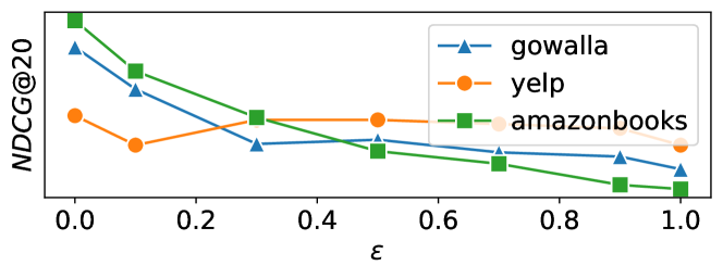
Figure 1: Empirical results on $\epsilon$ tuning. ($\lambda$ is fixed according to performance, typically around 1.1.)

Relationship to Decoupled Contrastive Learning (DCL): Contrastive learning fundamentally operates by treating two augmented ”views” of an identical image or representation as positives to be drawn nearer, while considering all others as negatives to be distanced. By removing negative-positive-coupling (NPC) effect in the prevalent InfoNCE loss, (Yeh et al. 2022) proposed Decoupled Contrastive Learning (DCL) loss which discards the positive term from the denominator and proved to improve the learning efficiency significantly. Formally, we write DCL as follows in the recommendation setting:

$$\begin{split}\widetilde{\mathcal{L}}_{dcl}=-\operatorname*{\mathbb{E}}_{u}\sum\limits_{i\in I_{u}^{+}}\Big{(}\hat{y}_{ui}-\log\sum\limits_{j=1;j\sim p_{u}^{-}}^{N}exp(\hat{y}_{uj})\Big{)}\end{split}$$ (7)

As discussed above, this formula coincides with Eq. 6 when $\lambda=1$ and $\epsilon=0$. Intuitively, removing the positive from the denominator gives a larger weight to the hard positives and tends to increase the representation quality. Interestingly, this loss can be further explained from the perspective of mutual information (Belghazi et al. 2018).

Relationship to Mutual Information Neural Estimator (MINE) Here, we first introduce a Mutual Information Neural Estimator (MINE) loss and show it is the equivalence of decoupling. The MINE loss is introduced in  (Belghazi et al. 2018), which can directly measure the mutual information between user and item:

$$\widehat{I(u,i)}=sup_{(v_{u};v_{i})}\operatorname*{\mathbb{E}}_{p_{u,i}}[\hat{y}_{ui}]-\log\operatorname*{\mathbb{E}}_{p_{u}\otimes p_{i}}[e^{\hat{y}_{ui}}]$$ (8)

Here, the positive $\hat{y}_{ui}$ items sampled $n$ times according to the joint user-item distribution $p_{u,i}$. The negative items are sampled according to the empirical marginal item distribution of $p_{i}$, which are proportional to their popularity (or in practice, sampled uniformly). A simple adaption of MINE to the recommendation setting can be formalized as:

$$\begin{split}\mathcal{L}_{mine}&=-\operatorname*{\mathbb{E}}_{u}\operatorname*{\mathbb{E}}_{i\sim p_{u}^{+}}\Bigg{[}\hat{y}_{ui}-\log\operatorname*{\mathbb{E}}_{j\sim p_{i}}[\exp\hat{y}_{uj}]\Bigg{]}\end{split}$$ (9)

This is the same as Eq. 7 (the factor of expectation will not affect the optimization). And to the best of our knowledge, this work is the first to study and apply MINE (Belghazi et al. 2018) to the recommendation setting.

Simplified Contrastive Learning: MINE+

Ultimately, with the support of our empirical study and the theoretical foundation of decoupled contrastive learning as well as MINE, we propose the following simplified InfoNCE+ (Eq. 6, which is referred to as MINE+:

$$\boxed{\begin{split}\widetilde{\mathcal{L}}_{mine+}=-\operatorname*{\mathbb{E}}_{u}\sum\limits_{i\sim p_{u}^{+}}&\Bigg{[}{\hat{y}_{ui}}-\lambda\log\sum_{j=1;j\sim p_{i}}^{N}\exp{\hat{y}_{uj}}\Bigg{]}\end{split}}$$ (10)

In addition, $\hat{y}_{ui}$ can be adopted as cosine similarity between user and item latent vectors, i.e., cosine ($<v_{u}/||v_{u}||,v_{i}/||v_{i}||>$), then $\hat{y}_{ui}$ is normalized by a temperature, such as $<v_{u}/||v_{u}||,v_{i}/||v_{i}||>/t$. Note that such treatment of using temperature is a common practice for the contrastive learning (Chen et al. 2020). Our experimental results also confirm such treat can help boost the performance for recommendation as well.

Lower Bound Analysis

In this subsection, we theoretically discuss some common lower bounds for InfoNCE and MINE (aka DCL), BPR as well as their relationship.

Given Equation 9, we can easily observe (based on Jensen’s inequality):

$$\begin{split}&\widetilde{\mathcal{L}}_{info}=-\operatorname*{\mathbb{E}}_{u}\operatorname*{\mathbb{E}}_{i\sim p_{u}^{+}}\log\frac{exp(\hat{y}_{ui})}{exp(\hat{y}_{ui})+\sum_{j=1;j\sim p_{u}}^{N}exp(\hat{y}_{uj})}\geq\\ &\widetilde{\mathcal{L}}_{mine}=\operatorname*{\mathbb{E}}_{u}\operatorname*{\mathbb{E}}_{i\sim p_{u}^{+}}\log(\sum_{j=1;j\sim p_{i}}^{N}exp(\hat{y}_{uj}-\hat{y}_{ui}))\approx\\ &\operatorname*{\mathbb{E}}_{u}\operatorname*{\mathbb{E}}_{i\sim p_{u}^{+}}\log N\operatorname*{\mathbb{E}}_{j\sim p_{i}}exp(\hat{y}_{uj}-\hat{y}_{ui}))\geq\\ &\operatorname*{\mathbb{E}}_{u}\operatorname*{\mathbb{E}}_{i\sim p_{u}^{+}}\operatorname*{\mathbb{E}}_{j\sim p_{i}}\bigl{(}\hat{y}_{uj}-\hat{y}_{ui}\bigr{)}+\log N\geq\operatorname*{\mathbb{E}}_{u}\operatorname*{\mathbb{E}}_{i\sim p_{u}^{+}}\operatorname*{\mathbb{E}}_{j\sim p_{i}}\bigl{(}\hat{y}_{uj}-\hat{y}_{ui}\bigr{)}\end{split}$$ (11)

Alternative, by using LogSumExp lower-bound (Barbano et al. 2023), we also observe:

$$\begin{split}&\operatorname*{\mathbb{E}}_{u}\operatorname*{\mathbb{E}}_{i\sim p_{u}^{+}}\max_{j=1;j\sim p_{i}}^{N}\bigl{(}0,\hat{y}_{uj}-\hat{y}_{ui}\bigr{)}+\log(N+1)\geq\\ &\widetilde{\mathcal{L}}_{info}\geq\widetilde{\mathcal{L}}_{mine}=\operatorname*{\mathbb{E}}_{u}\operatorname*{\mathbb{E}}_{i\sim p_{u}^{+}}\log(\sum_{j=1;j\sim p_{i}}^{N}exp(\hat{y}_{uj}-\hat{y}_{ui}))\geq\\ &\operatorname*{\mathbb{E}}_{u}\operatorname*{\mathbb{E}}_{i\sim p_{u}^{+}}\max_{j=1;j\sim p_{i}}^{N}\bigl{(}\hat{y}_{uj}-\hat{y}_{ui}\bigr{)}\end{split}$$ (12)

Note that the second lower bound is tighter than the first one. And it is obvious to observe that the looser bound Eq. 11 is also shared by the well-known pairwise BPR loss (Eq. 1), which aims to maximize the average difference between a positive item score ($\hat{y}_{ui}$) and a negative item score ($\hat{y}_{uj}$).

However, the tighter lower bound of BPR diverges from the one shared by InfoNCE and MINE loss (Eq. 12) using the LogSumExp lower bound:

$$\begin{split}&\widetilde{\mathcal{L}}_{bpr}=\operatorname*{\mathbb{E}}_{u}\operatorname*{\mathbb{E}}_{i\sim p_{u}^{+}}\sum_{j=1;j\sim p_{i}}^{N}\log(1+exp(\hat{y}_{uj}-\hat{y}_{ui}))\geq\\ &\operatorname*{\mathbb{E}}_{u}\operatorname*{\mathbb{E}}_{i\sim p_{u}^{+}}\sum_{j=1;j\sim p_{i}}^{N}max(0,\hat{y}_{uj}-\hat{y}_{ui})\varpropto\\ &\operatorname*{\mathbb{E}}_{u}\operatorname*{\mathbb{E}}_{i\sim p_{u}^{+}}\operatorname*{\mathbb{E}}_{j\sim p_{i}}max(0,\hat{y}_{uj}-\hat{y}_{ui})\end{split}$$ (13)

Note that the bound in Eq. 13 only sightly improves over the one in Eq. 11 and cannot reflect the tight bounds (Eq. 12) shared by InfoNCE and MINE, which aims to minimize the largest gain of a negative item (random) over a positive item ($\max_{j=1;j\sim p_{i}}^{N}\bigl{(}\hat{y}_{uj}-\hat{y}_{ui}\bigr{)}$).

This bound (Eq. 12) provides a deeper understanding of the contrastive learning loss, which aims to minimize the largest gain of a negative item (random) over a positive item ($\max_{j=1;j\sim p_{i}}^{N}\bigl{(}\hat{y}_{uj}-\hat{y}_{ui}\bigr{)}$).

Debiased Contrastive Recommendation Loss

In  (Chuang et al. 2020), a novel debiased estimator is proposed while only accessing positive items and unlabeled training data. Below, we demonstrate how this approach can be adopted in the recommendation setting.

Given user $u$, let us consider the implicit (binary) preference probability (class distribution) of $u$: $\rho_{u}(c)$, where $\rho_{u}(c=+)=\tau^{+}_{u}$ represents the probability of user $u$ likes an item, and $\rho_{u}(c=-)=\tau^{-}_{u}=1-\tau^{+}_{u}$ corresponds to being not interested. In the recommendation set, we may consider $\rho_{u}(+)$ as the fraction of positive items, i.e., those top $K$ items, and $\rho_{u}(-)$ are the fraction of true negative items. Let the item class joint distribution be $p_{u}(i,c)=p_{u}(i|c)\rho_{u}(c)$. Then $p^{+}_{u}(i)=p_{u}(i|c=+)$ is the probability of observing $i$ as a positive item for user $u$ and $p_{u}^{-}(j)=p_{u}(j|c=-)$ the probability of a negative example. Given this, the distribution of an individual item of user $u$ is:

$$\begin{split}p_{u}(i)=\tau^{+}_{u}\cdot p^{+}_{u}(i)+\tau^{-}_{u}\cdot p_{u}^{-}(i)\end{split}$$ (14)

Assume the known positive items $\mathcal{I}_{u}^{+}$ are being uniformly sampled according to $p^{+}_{u}$. For $\tau^{+}_{u}$, we can count all the existing positive items ($r_{ui}=1$), and the unknown top $K$ items as being positive, thus, $\tau^{+}_{u}=(|\operatorname*{\mathcal{I}}_{u}^{+}|+K)/|\mathcal{I}|$. Alternatively, we can also assume the number of total positive items for $u$ is proportional to the number of existing (known) positive items, i.e, $\tau^{+}_{u}=(1+\alpha)|\operatorname*{\mathcal{I}}_{u}^{+}|/|\mathcal{I}|$, where $\alpha\geq 0$. As mentioned earlier, the typical assumption of $p_{u}$ (the probability distribution of selection of an item is also uniform). Then, we can represent $p^{-}_{u}$ using the total and positive sampling as: $p^{-}_{u}(i)=1/\tau^{-}_{u}(p_{u}(i)-\tau^{+}_{u}\cdot p^{+}_{u}(i))$. Upon these assumptions, let us consider the following ideal (debiased) InfoNCE loss:

$$\begin{split}\overline{\mathcal{L}}_{Info}&=-\operatorname*{\mathbb{E}}_{u}\operatorname*{\mathbb{E}}_{i\sim p_{u}^{+}}\Bigg{[}\log\frac{\exp(\hat{y}_{ui})}{\exp(\hat{y}_{ui})+\lambda_{n}\operatorname*{\mathbb{E}}_{j\sim p_{u}^{-}}\exp({\hat{y}_{uj}})}\Bigg{]}\\ &=-\operatorname*{\mathbb{E}}_{u}\operatorname*{\mathbb{E}}_{i\sim p_{u}^{+}}\Bigg{[}\log\frac{\exp(\hat{y}_{ui})}{\exp(\hat{y}_{ui})+\lambda_{n}\frac{1}{\tau^{-}}T}\Bigg{]}\\ T&=\Big{(}\operatorname*{\mathbb{E}}_{t\sim p_{u}}[\exp(\hat{y}_{ut})]-\tau^{+}\operatorname*{\mathbb{E}}_{j\sim p^{+}_{u}}[\exp(\hat{y}_{uj})]\Big{)}\end{split}$$ (15)

Note that when $\lambda_{n}=N$, the typical InfoNCE loss $\mathcal{L}_{Info}$ (Eq. 4) converges into $\overline{\mathcal{L}}_{Info}$ when $N\rightarrow\infty$. Now, we can use $N$ samples from $p_{u}$ (not negative samples), an $M$ positive samples from $p_{u}^{+}$ to empirically estimate $\overline{\mathcal{L}}_{Info}$ following  (Chuang et al. 2020):

$$\begin{split}\mathcal{L}^{Debiased}_{Info}=-\operatorname*{\mathbb{E}}_{u}\operatorname*{\mathbb{E}}_{\begin{subarray}{c}i\sim p_{u}^{+};\\ j\sim p_{u};\\ k\sim p_{u}^{+}\end{subarray}}\Bigg{[}\log\frac{\exp(\hat{y}_{ui})}{\exp(\hat{y}_{ui})+\lambda_{n}f(\{j\}_{1}^{N},\{k\}_{1}^{M})}\Bigg{]}\end{split}$$ (16)

$f(\{j\}_{1}^{N},\{k\}_{1}^{M})=\max\Bigl{\{}\frac{1}{\tau_{u}^{-}}\Bigl{(}\frac{1}{N}\sum_{j=1;j\sim p_{u}}^{N}exp(f_{uj})-\tau_{u}^{+}\frac{1}{M}\sum_{k=1;k\sim p_{u}^{+}}^{M}exp(f_{uk})\Bigr{)},e^{1/t}\Bigr{\}}$. Here $f$ is constrained to be greater than its theoretical minimum $e^{-1/t}$ to prevent the negative number inside $\log$. We will experimentally study this debiased InfoNCE in a later section.

Debiased CCL

Following the analysis of debiased contrastive learning, clearly, some of the positive items are unlabeled, and making them closer to $0$ is not the ideal option. In fact, if the optimization indeed reaches the targeted score, we actually do not learn any useful recommendations. A natural question is whether we can improve other contrastive learning loss (for example, cosine contrastive loss (CCL) (Mao et al. 2021)) following the debiased contrastive learning paradigm  (Chuang et al. 2020)?

The cosine contrastive loss (CCL) is a recently proposed loss and has shown to be very effective for recommendation (Mao et al. 2021). The original Contrastive Cosine Loss (CCL) (Mao et al. 2021) can be written as:

$$\begin{split}\mathcal{L}_{ccl}=\operatorname*{\mathbb{E}}_{u}\Bigg{(}\sum\limits_{i\in\mathcal{I}^{+}_{u}}(1-\hat{y}_{ui})+\frac{w}{N}\sum\limits_{j\in\mathcal{I}}^{N}ReLU(\hat{y}_{uj}-\epsilon_{0})\Bigg{)}\end{split}$$ (17)

where $\hat{y}_{uj}$ is cosine similarity, $ReLU(x)=max(0,x)$ is the activation function, $w$ is the negative weight, $N$ is the number of negative samples and $\epsilon_{0}$ is margin.

Definition 1.

(Ideal CCL Loss) The ideal CCL loss function for recommendation models is the expected single pointwise loss for all positive items (sampled from $\rho_{u}(+)=\tau^{+}$) and for negative items (sampled from $\rho_{u}(-)=\tau^{-}$):

$$\overline{\mathcal{L}}_{ccl}=\operatorname*{\mathbb{E}}_{u}\Bigg{(}\tau_{u}^{+}\operatorname*{\mathbb{E}}_{i\sim p_{u}^{+}}(1-\hat{y}_{ui})+\lambda_{n}\cdot\tau_{u}^{-}\operatorname*{\mathbb{E}}_{j\sim p_{u}^{-}}[ReLU(\hat{y}_{uj}-\epsilon_{0})]\Bigg{)}$$ (18)

Why this is ideal? When the optimization reaches the potential minimal, we have all positive items $i$ and all the negative items $j$ reaching all the minimum of individual loss ($l^{+}$ and $l^{-}$). Here, $\lambda_{n}$ help adjusts the balance between the positive and negative losses. However, since $p_{u}^{+}$ and $p_{u}^{-}$ are unknown, we utilize the same debiase approach as InfoNCE  (Oord, Li, and Vinyals 2018).

Definition 2.

(Debiased CCL loss)

$$\boxed{\begin{split}&\mathcal{L}^{debiased}_{CCL}=\operatorname*{\mathbb{E}}_{u}\Bigg{(}\tau_{u}^{+}\operatorname*{\mathbb{E}}_{i\sim p_{u}^{+}}(1-\hat{y}_{ui})\\ &+\lambda_{n}\Big{(}\operatorname*{\mathbb{E}}_{j\sim p_{u}}[ReLU(\hat{y}_{uj}-\epsilon)]-\tau_{u}^{+}\operatorname*{\mathbb{E}}_{k\sim p^{+}_{u}}[ReLU(\hat{y}_{uk}-\epsilon_{0})]\Big{)}\Bigg{)}\\ \end{split}}$$ (19)

In practice, for the computation of expectation, we sample $N$ positive items and $M$ negative items to obtain an empirical loss.

iALS and EASE are debiased

Besides the typical InfoNCE as well as cosine contrastive learning loss, another most commonly used loss is Mean-Square-Error (MSE), as well as the well-known quadratic linear models - iALS (Rendle et al. 2022; Hu, Koren, and Volinsky 2008b) and EASE (Steck 2019). We may wonder whether they are biased or not. Surprisingly, we found these linear models are naturally debiased which contributes to the following observation:

Observation 1.

The solvers of both iALS and EASE models can absorb their debiased counterparts under existing frameworks with reasonable conditions.

This observation reflects the outstanding performances of simple linear models from the debias angle, which coincide with the recent series of fundamental revisiting works (Rendle et al. 2022; Dacrema, Cremonesi, and Jannach 2019; Jin et al. 2021a). For detailed proof and explanation please see Theorem 1 and Theorem 2 and their proofs in technical supplementary.

Table 1: Performance comparison to widely used models. We highlight the top-2 best models in each column. Results of models marked with $*$ are duplicated from (Mao et al. 2021) for consistency. For a fair comparison, MF-based models marked with $**$ are reproduced by ourselves with thorough parameter searching.

Model	Yelp		Gowalla		Amazon-Books
	Recall@20	NDCG@20	Recall@20	NDCG@20	Recall@20	NDCG@20
Deep Learning Based
YouTubeNet* (Covington, Adams, and Sargin 2016)	6.86	5.67	17.54	14.73	5.02	3.88
NeuMF* (He et al. 2017)	4.51	3.63	13.99	12.12	2.58	2
CML* (Hsieh et al. 2017)	6.22	5.36	16.7	12.92	5.22	4.28
MultiVAE* (Liang et al. 2018)	5.84	4.5	16.41	13.35	4.07	3.15
LightGCN* (He et al. 2020)	6.49	5.3	18.3	15.54	4.11	3.15
NGCF* (Wang et al. 2019)	5.79	4.77	15.7	13.27	3.44	2.63
GAT* (Veličković et al. 2018)	5.43	4.32	14.01	12.36	3.26	2.35
PinSage* (Ying et al. 2018)	4.71	3.93	13.8	11.96	2.82	2.19
SGL-ED* (Wu et al. 2021)	6.75	5.55	-	-	4.78	3.79
MF based
iALS** (Rendle et al. 2022)	6.06	5.02	13.88	12.24	2.79	2.25
MF-BPR** (Rendle et al. 2009)	5.63	4.60	15.90	13.62	3.43	2.65
MF-CCL** (Mao et al. 2021)	6.91	5.67	18.17	14.61	5.27	4.22
MF-CCL-debiased (ours)	6.98	5.71	18.42	14.97	5.49	4.40
MF-MINE+ (ours)	7.20	5.92	18.53	15.70	5.31	4.14

Experiment

In this section, we experimentally study the newly proposed MINE+ loss as well as the existing recommendation loss w.r.t their corresponding debiased ones. This could help better understand and compare the resemblance and discrepancy between different loss functions in the perspective of contrastive learning. Specifically, we would like to answer the following questions:

• Q1. How does our proposed MINE+ objective function compare to widely used ones?

• Q2. How does the bias introduced by the existing negative sampling impact model performance and how do our proposed debiased losses perform compared to traditional biased ones?

• Q3. What is the effect of different hyperparameters on the contrastive learning loss functions?

Experimental Setup

Datasets We examed three commonly used datasets, Amazon-Books, Yelp2018 and Gowalla by a number of recent studies (Mao et al. 2021; He et al. 2020; Wang et al. 2019; Wu et al. 2021). We obtain the publicly available processed data and follow the same setting as (Wang et al. 2019; He et al. 2020; Mao et al. 2021).

Evaluation Metrics Consistent with benchmarks (Wang et al. 2019; He et al. 2020; Mao et al. 2021), we evaluate the performance by $Recall@20$ and $NDCG@20$ over all items (Krichene and Rendle 2020; Jin et al. 2021b; Li et al. 2023a, 2020, b).

Models This paper focuses on the study of loss functions, which is architecture agnostic. Thus, we evaluate our loss functions on top of the simplest one - Matrix Factorization (MF) in this study. By eliminating the influence of the architecture, we can compare the power of various loss functions fairly. Meantime, we compare the performance of the proposed methods with a few classical machine learning models as well as advanced deep learning models, including, iALS (Rendle et al. 2022), MF-BPR(Rendle et al. 2009), MF-CCL (Mao et al. 2021), YouTubeNet (Covington, Adams, and Sargin 2016), NeuMF (He et al. 2017), LightGCN (He et al. 2020), NGCF (Wang et al. 2019), CML (Hsieh et al. 2017), PinSage (Ying et al. 2018), GAT (Veličković et al. 2018), MultiVAE (Liang et al. 2018), SGL-ED (Wu et al. 2021). Those comparisons can help establish that the loss functions with basic MF can produce strong and robust baselines for the recommendation community to evaluate more advanced and sophisticated models.

Loss functions As the core of this paper, we focus on some most widely used loss functions and their debiased counterparts, including InfoNCE (Oord, Li, and Vinyals 2018), MSE (Hu, Koren, and Volinsky 2008b; Rendle et al. 2022), and state-of-the-art CCL (Mao et al. 2021), as well as our new proposed MINE+ (Belghazi et al. 2018; Yeh et al. 2022).

Reproducibility To implement reliable models, by default, we set batch size as $512$. Adam optimizer learning rate is initially set as $1e-4$ and reduced by $0.5$ on the plateau, early stopped until it arrives at $1e-6$. For the cases where negative samples get involved, we would set it as $800$ by default. We search the global regularization weight between $1e-9$ to $1$ with an increased ratio of $10$. To ensure the reproducibility, for the exact hyperparameter settings of the model, we would present it in the technical appendix and our anonymous code is also available at https://anonymous.4open.science/r/AAAI-2024-Anonymous-9B33/README.md.

Table 2: The performance of different loss functions w.r.t their debiased ones on MF. The unit of the metric values is $\%$. We also present and highlight the relative improvement (RI) of the debiased loss function with its vanilla (biased) counterpart.

Loss		Yelp		Gowalla		Amazon-Books		Average RI%
		Recall@20	NDCG@20	Recall@20	NDCG@20	Recall@20	NDCG@20
CCL	biased	6.91	5.67	18.17	14.61	5.27	4.22	-
	debiased	6.98	5.71	18.42	14.97	5.49	4.40	-
	RI%	1.01%	0.71%	1.38%	2.46%	4.17%	4.27%	2.33%
InfoNCE	biased	6.54	5.36	16.45	13.43	4.60	3.56	-
	debiased	6.66	5.45	16.57	13.72	4.65	3.66	-
	RI%	1.83%	1.68%	0.73%	2.16%	1.09%	2.81%	1.72%
MINE (ours)	MINE	6.56	5.37	16.93	14.28	5.00	3.93	-
	RI% (w.r.t biased infoNCE)	0.31%	0.19%	2.92%	6.33%	8.70%	10.39%	4.80%
	MINE+	7.20	5.92	18.53	15.70	5.31	4.14	-
	RI% (w.r.t biased infoNCE)	10.09%	10.45%	12.64%	16.90%	15.43%	16.29%	13.63%

Q1. Performance of MINE/MINE+

First, we delve into the examination of the newly proposed MINE+ loss function (Eq. 10). As mentioned before, to our best knowledge, this is the first study utilizing MINE/MINE+ aka decoupled contrastive learning loss in recommendation settings. In Table 1, we can observe MF-MINE+, as well as debiased MF-CCL, perform best or second best in most cases, affirming the superiority of the MINE+ loss and debiased CCL. Then, We compare MINE/MINE+ with other loss functions (CCL, InfoNCE), all set MF as the backbone, as displayed in (Table 2,. Our results show the surprising effectiveness of MINE-type losses. In particular, the basic MINE is shown close to $4.8\%$ average lifts over the (biased) InfoNCE loss, a rather stand loss in recommendation models. MINE+ even demonstrates superior performance compared to the state-of-the-art CCL loss function. Furthermore, MINE+ consistently achieves better results than InfoNCE with a maximum improvement of 16% (with an average improvement over $14\%$.

These findings highlight the potential of MINE as an effective objective function for recommendation models and systems. Noting that our MINE+ loss is model agnostic, which can be applied to any representation-based model. We leave the study of combining MINE.MINE+ models with more advanced (neural) architecture in future studies.

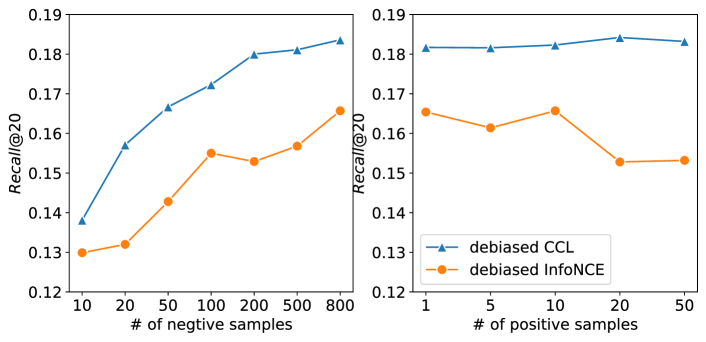
Figure 2: Effect of number of samples on $Gowalla$

Q2. (Biased) Loss vs Debiased Loss

Here, we seek to examine the negative impact of bias introduced by negative sampling and assess the effectiveness of our proposed debiased loss functions. We utilize Matrix Factorization (MF) as the backbone and compare the performance of the original (biased) version and the debiased version for the loss functions of $CCL$ (Mao et al. 2021) and $InfoNCE$ (Oord, Li, and Vinyals 2018). Table 2 shows the biased loss vs debiased loss (on top of the MF) results.

The results show that the debiased methods consistently outperform the biased ones for the CCL and InfoNCE loss functions in all cases. In particular, the debiased method exhibits remarkable improvements of up to over $4\%$ for the CCL loss function on the Amazon-Books dataset. This highlights the adverse effect of bias in recommendation quality and demonstrates the success of applying contrastive learning based debiase methods in addressing this issue. Finally, we note that the performance gained by the debiased losses is also consistent with the results over other machine learning tasks as shown in  (Chuang et al. 2020).

Q3. Hyperparameter analysis

First, we analyze the impacts of hyperparameters in the debiased framework (Eqs. 16 and 19): negative weight $\lambda_{n}$, number of negative samples, and number of positive samples as shown in Figs. 2 and 3. The left side of Fig. 2 reveals that increasing the number of negative samples leads to better performance in models overall. The right side of Fig. 2 shows that the number of positive samples in the debiased formula has a minor impact on performance compared to negative samples. In Fig. 3, we illustrate how the negative weight $\lambda_{n}$ affects the performance of the debiased InfoNCE (Eq. 16). In general, we observe the $\cap$ shaped curve for quality metric ($Recall@20$ here) for the parameters. In Fig. 4, we investigate how noise weight $\lambda$ in Eq. 10 can affect the performance of the $MINE+$ loss function. In general, it would achieve optimal around $1.1\sim 1.2$ for all datasets.

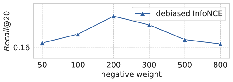
Figure 3: Effect of negative weight $\lambda_{0}$ on debiased InfoNCE loss $Gowalla$

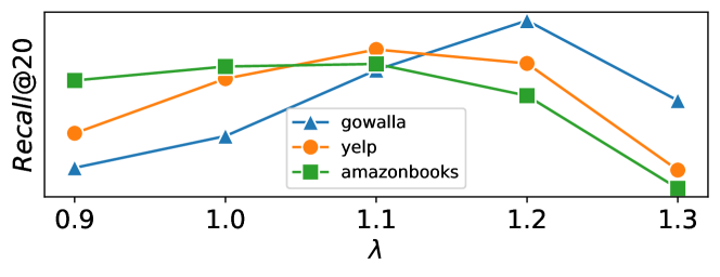
Figure 4: Effect of noise weight $\lambda$ in MINE+ loss on $Gowalla$

conclusion

In this paper, we conduct a comprehensive analysis of recommendation loss functions from the perspective of contrastive learning. Two novel recommendation losses MINE+ and Debiased CCL are developed through investigation into and integration with the contrastive learning losses. Both iALS and EASE are certified to be inherently debiased. The empirical experimental results demonstrate the debiased losses and new information losses outperform the existing (biased) ones. In the future, we would like to investigate how effective does the loss functions work with more sophisticated neural architectures and seek additional theoretical evidence on why MINE+ performs better than other losses, such as SoftMax.

Appendix A Related Work

Objectives of Implicit Collaborative Filtering

Implicit feedback has been popular for decades in Recommender System (Rendle 2021) since Hu et al. first proposed iALS (Hu, Koren, and Volinsky 2008b), where a second-order pointwise objective - Mean Square Error (MSE) was adopted to optimize user and item embeddings alternatively. Due to its effectiveness and efficiency, there is a large number of works that take the MSE or its variants as their objectives, spanning from Matrix Factorization (MF) based models (Rendle et al. 2022, 2021; He et al. 2016), to regression-based models, including SLIM (Ning and Karypis 2011), EASE (Steck 2019, 2020), etc. He et al. treat collaborative filtering as a binary classification task and apply the pointwise objective - Binary Cross-Entropy Loss (BCE) onto it (He et al. 2017). CML utilized the pairwise hinge loss onto the collaborative filtering scenario (Hsieh et al. 2017). MultiVAE (Liang et al. 2018) utilizes multinomial likelihood estimation. Rendle et al. proposed a Bayesian perspective pairwise ranking loss - BPR, in the seminal work (Rendle et al. 2009). YouTubeNet posed a recommendation as an extreme multiclass classification problem and apply the Softmax cross-entropy (Softmax) (Covington, Adams, and Sargin 2016; Jean et al. 2015). Recently, inspired by the largely used contrastive loss in the computer vision area, (Mao et al. 2021) proposed a first-order based Cosine Contrastive Loss (CCL), where they maximize the cosine similarity between the positive pairs (between users and items) and minimize the similarity below some manually selected margin.

Contrastive Learning

Recently, Contrastive Learning (CL) (Chen et al. 2020; Oord, Li, and Vinyals 2018) has become a prominent optimizing framework in deep learning and machine learning (Li et al. 2022; Wu et al. 2018; Wu, Ye, and Man 2023; Li, Bhargavi, and Ravipati 2023). The motivation behind CL is to learn representations by contrasting positive and negative pairs as well as maximize the positive pairs, including data augmentation (Chen et al. 2020) and multi-view representations (Tian, Krishnan, and Isola 2020), etc. Chuang et al. proposed a new unsupervised contrastive representation learning framework, targeting to minimize the bias introduced by the selection of the negative samples. This debiased objective consistently improved its counterpart - the biased one in various benchmarks (Chuang et al. 2020). Lately, by introducing the margin between positive and negative samples, Belghazi et al. present a supervised contrastive learning framework that is robust to biases (Barbano et al. 2023). In addition, a mutual information estimator - MINE (Belghazi et al. 2018), closely related to the contrastive learning loss InfoNCE(Oord, Li, and Vinyals 2018), has demonstrated its efficiency in various optimizing settings. (Wang et al. 2022) study the alignment and uniformity of user, item embeddings from the perspective of contrastive learning in the recommendation. CLRec (Zhou et al. 2021) design a new contrastive learning loss which is equivalent to using inverse propensity weighting to reduce exposure bias of a large-scale system.

Negative Sampling Strategies for Item Recommendation

In most real-world scenarios, only positive feedback is available which brings demand for negative signals to avoid trivial solutions during training recommendation models. Apart from some non-sampling frameworks like iALS (Hu, Koren, and Volinsky 2008b), Multi-VAE (Liang et al. 2018), the majority of models (Chen et al. 2022a; He et al. 2020, 2017; Rendle et al. 2009; Rendle 2021; Chen et al. 2017) would choose to sample negative items for efficiency consideration. Uniform sampling is the most popular one (Rendle et al. 2009) which assumes uniform prior distribution. Importance sampling is another popular choice (Lian, Liu, and Chen 2020), which chooses negative according to their frequencies. Adaptive sampling strategy keep tracking and picking the negative samples with higher scores (Rendle and Freudenthaler 2014; Zhang et al. 2013). Another similar strategy is SRNS (Ding et al. 2020), which tries to find and optimize false negative samples In addition, NCE (Gutmann and Hyvärinen 2010) approach for negative sampling has also been adopted in the recommendation system(Chen et al. 2017).

Bias and Debias in Recommendation

In the recommender system, there are various different bias (Chen et al. 2022b), including item exposure bias, popularity bias, position bias, selection bias, etc. These issues have to be carefully handled otherwise it would lead to unexpected results, such as inconsistency of online and offline performance, etc. Marlin et al. (Marlin et al. 2007) validate the existence of selection bias by conducting a user survey, which indicates the discrepancy between the observed rating data and all data. Since users are generally exposed to a small set of items, unobserved data doesn’t mean negative preference, this is so-called exposure bias (Liu et al. 2020). Position bias (Collins et al. 2018) is another commonly encountered one, where users are more likely to select items that display in a desirable place or higher position on a list.

Steck et al. (Steck 2010) propose an unbiased metric to deal with selection bias. iALS (Hu, Koren, and Volinsky 2008b) put some weights on unobserved data which helps improve the performance and deal with exposure bias. In addition, the sampling strategy would naturally diminish the exposure bias during model training (Chen et al. 2022b; Rendle et al. 2009). EXMF (Liang et al. 2016) is a user exposure simulation model that can also help reduce exposure bias. To reduce position bias, some models (Chapelle and Zhang 2009; Craswell et al. 2008) make assumptions about user behaviors and estimate true relevance instead of directly using clicked data. (Saito 2020) proposed an unbiased pairwise BPR estimator and further provide a practical technique to reduce variance. Another widely used method to correct bias is the utilization of propensity score (Zhu et al. 2020; Saito et al. 2020) where each item is equiped with some position weight.

Appendix B reproducibility

Table 3: Statistics of the datasets.

Dataset	User #	Item #	Interaction #
Yelp2018	31,668	38,048	$1,561,406$
Gowalla	29,858	40,981	$1,027,370$
Amazon-Books	52,643	91,599	$2,984,108$

Implement details

In Table 4, we list the details of the hyperparameters for reproducing the results of MINE+ (Eq. 10) in Tables 1 and 2.

In Table 5, we list the details of the hyperparameters for reproducing the results of debiased $CCL$ in Table 2.

Table 4: Hyperparameter details of $MINE+$ loss

	Yelp2018	Gowalla	Amazon-Books
negative weight	1.1	1.2	1.1
temperature	0.5	0.4	0.4
regularization	1	1	0.01
number of negative	800	800	800

Table 5: Hyperparameter details of debiased $CCL$ loss

	Yelp2018	Gowalla	Amazon-Books
negative weight	0.4	0.7	0.6
margin	0.9	0.9	0.4
regularization	-9	-9	-9
number of negative	800	800	800
number of positive	10	20	50

Appendix C MASE, iALS, EASE and their Debiasness

Let us denote the generic single pointwise loss function $l^{+}(\hat{y}_{ui})$ and $l^{-}(\hat{y}_{ui})$, which measure how close the individual positive (negative) item score to their ideal target value.

MSE single pointwise loss: Mean-Squared-Error (MSE) is one of the most widely used recommendation loss functions. Indeed, all the earlier collaborative filtering (Matrix factorization) models and pointwise losses were based on MSE (with different regularizations). Some recent linear models, such as SLIM (Ning and Karypis 2011) and EASE (Steck 2019), are also based on MSE. Its single pointwise loss function is denoted as:

$$\begin{cases}&l^{+}_{mse}(\hat{y}_{ui})=(1-\hat{y}_{ui})^{2}\\ &l^{-}_{mse}(\hat{y}_{ui})=(\hat{y}_{ui})^{2}\end{cases}$$ (20)

Definition 3.

(Ideal Pointwise Loss) The ideal pointwise loss function for recommendation models is the expected single pointwise loss for all positive items (sampled from $\rho_{u}(+)=\tau^{+}$) and for negative items (sampled from $\rho_{u}(-)=\tau^{-}$):

$$\begin{split}\overline{\mathcal{L}}_{point}=\operatorname*{\mathbb{E}}_{u}\Bigg{(}\tau_{u}^{+}\operatorname*{\mathbb{E}}_{i\sim p_{u}^{+}}l^{+}(\hat{y}_{ui})+\lambda\tau_{u}^{-}\operatorname*{\mathbb{E}}_{j\sim p_{u}^{-}}l^{-}(\hat{y}_{uj})\Bigg{)}\end{split}$$ (21)

Why this is ideal? When the optimization reaches the potential minimal, we have all positive items $i$ and all the negative items $j$ reaching all the minimum of individual loss ($l^{+}$ and $l^{-}$). Here, $\lambda$ help adjusts the balance between the positive and negative losses, similar to iALS  (Hu, Koren, and Volinsky 2008a; Rendle et al. 2022) and CCL (Mao et al. 2021). However, since $p_{u}^{+}$ and $p_{u}^{-}$ is unknown, we utilize the same debiasing approach as InfoNCE  (Oord, Li, and Vinyals 2018) for the debiased MSE:

Definition 4.

(Debiased Ideal pointwise loss)

$$\begin{split}&\mathcal{L}^{Debiased}_{point}=\operatorname*{\mathbb{E}}_{u}\Bigl{(}\tau_{u}^{+}\operatorname*{\mathbb{E}}_{i\sim p_{u}^{+}}l^{+}(\hat{y}_{ui})+\tau_{u}^{-}\lambda\cdot\operatorname*{\mathbb{E}}_{j\sim p_{u}^{-}}l^{-}(\hat{y}_{ui})\Bigr{)}\\ &=\operatorname*{\mathbb{E}}_{u}\Big{(}\tau_{u}^{+}\operatorname*{\mathbb{E}}_{i\sim p_{u}^{+}}l^{+}(\hat{y}_{ui})+\lambda\Big{(}\operatorname*{\mathbb{E}}_{j\sim p_{u}}l^{-}(\hat{y}_{ui})-\tau_{u}^{+}\operatorname*{\mathbb{E}}_{k\sim k^{+}_{u}}l^{-}(\hat{y}_{uj})\Big{)}\Big{)}\end{split}$$ (22)

In practice, assuming for each positive item, we sample $N$ positive items and $M$ negative items, then the empirical loss can be written as:

$$\begin{split}&\widetilde{\mathcal{L}}^{Debiased}_{point}=\operatorname*{\mathbb{E}}_{u}E_{i\sim p_{u}^{+}}\Bigl{(}\tau_{u}^{+}l^{+}(\hat{y}_{ui})+\\ &\lambda\Bigl{(}\frac{1}{N}\sum_{j=1;j\sim p_{u}}^{N}l^{-}(\hat{y}_{uj})-\tau_{u}^{+}\frac{1}{M}\sum_{k=1;k\sim p_{u}^{+}}^{M}l^{-}(\hat{y}_{uk})\Bigr{)}\Bigr{)}\end{split}$$ (23)

Here, we investigate how the debiased MSE loss will impact the solution of two (arguably) most popular linear recommendation models, iALS  (Hu, Koren, and Volinsky 2008a; Rendle et al. 2022) and EASE (Steck 2019). Rather surprisingly, we found the solvers of both models can absorb the debiased loss under their existing framework with reasonable conditions (details below). In other words, both iALS and EASE can be considered to be inherently debiased.

To obtain the aforementioned insights, we first transform the debiased loss into the summation form being used in iALS and EASE.

$$\begin{split}&\mathcal{L}^{Debiased}_{mse}\approx\operatorname*{\mathbb{E}}_{u}\Bigg{[}\frac{\tau^{+}_{u}}{|\mathcal{I}^{+}_{u}|}\sum\limits_{i\in\mathcal{I}_{u}^{+}}(\hat{y}_{ui}-1)^{2}+\lambda\Bigg{(}\frac{1}{|\mathcal{I}|}\sum\limits_{t\in\mathcal{I}}\hat{y}_{ut}^{2}-\frac{\tau^{+}_{u}}{|\mathcal{I}_{u}^{+}|}\sum\limits_{q\in\mathcal{I}_{u}^{+}}\hat{y}^{2}_{uq}\Bigg{)}\Bigg{]}\\ &=\sum\limits_{u}\Bigg{[}\frac{1}{|\mathcal{I}|}c_{u}\sum\limits_{i\in\mathcal{I}_{u}^{+}}(\hat{y}_{ui}-1)^{2}\ \ \ \ \ \ \ \ \ \ \ \ \ \ \text{where, }c_{u}=\frac{|\mathcal{I}|}{|\mathcal{I}_{u}^{+}|}\tau_{u}^{+}\\ &+\lambda\Bigg{(}\frac{1}{|\mathcal{I}|}\sum\limits_{t\in\mathcal{I}}\hat{y}_{ut}^{2}-\frac{1}{|\mathcal{I}|}c_{u}\sum\limits_{q\in\mathcal{I}_{u}^{+}}\hat{y}^{2}_{uq}\Bigg{)}\Bigg{]}\\ &\propto\sum\limits_{u}\Bigg{[}c_{u}\sum\limits_{i\in\mathcal{I}_{u}^{+}}(\hat{y}_{ui}-1)^{2}+\lambda\Bigg{(}\sum\limits_{t\in\mathcal{I}}\hat{y}_{ut}^{2}-c_{u}\sum\limits_{q\in\mathcal{I}_{u}^{+}}\hat{y}^{2}_{uq}\Bigg{)}\Bigg{]}\\ &=\sum\limits_{u}\Bigg{[}\sum\limits_{i\in\mathcal{I}_{u}^{+}}[c_{u}(\hat{y}_{ui}-1)^{2}-c_{u}\lambda\hat{y}^{2}_{uq}]+\lambda\sum\limits_{t\in\mathcal{I}}\hat{y}_{ut}^{2}\Bigg{]}\end{split}$$

Debiased iALS: Following the original iALS paper (Hu, Koren, and Volinsky 2008b), and the latest revised iALS (Rendle et al. 2022, 2021), the objective of iALS is given by (Rendle et al. 2022):

$$\begin{split}\mathcal{L}_{iALS}&=\sum\limits_{(u,i)\in S}(\hat{y}(u,i)-1)^{2}+\alpha_{0}\sum\limits_{u\in U}\sum\limits_{i\in I}\hat{y}(u,i)^{2}\\ &+\lambda\Bigg{(}\sum\limits_{u\in U}(|\mathcal{I}_{u}^{+}|+\alpha_{0}|\mathcal{I}|)^{\nu}||\mathbf{w}_{u}||^{2}+\sum\limits_{i\in I}(|U_{i}^{+}|+\alpha_{0}|\mathcal{U}|)^{\nu}||\mathbf{h}_{i}||^{2}\Bigg{)}\end{split}$$ (24)

where $\lambda$ is global regularization weight (hyperparameter) and $\alpha_{0}$ is unobserved weight (hyperparameter). $\mu$ is generally set to be $1$. Also, $\mathbf{w}_{u}$ and $\mathbf{h}_{i}$ are user and item vectors for user $u$ and item $i$, respectively.

Now, we consider applying the debiased MSE loss to replace the original MSE loss (the first line in $\mathcal{L}_{iALS}$) with the second line unchanged:

$$\begin{split}&\mathcal{L}^{Debiased}_{iALS}=\sum\limits_{u\in U}\Bigg{[}\sum\limits_{i\in\mathcal{I}_{u}^{+}}[c_{u}(\hat{y}_{ui}-1)^{2}-c_{u}\cdot\alpha_{0}\cdot\hat{y}^{2}_{ui}]+\alpha_{0}\sum\limits_{t\in I}\hat{y}_{ut}^{2}\Bigg{]}\\ &+\lambda\Bigg{(}\sum\limits_{u\in U}(|\mathcal{I}_{u}^{+}|+\alpha_{0}|\mathcal{I}|)^{\nu}||\mathbf{w}_{u}||^{2}+\sum\limits_{i\in I}(|\mathcal{U}_{i}^{+}|+\alpha_{0}|\mathcal{U}|)^{\nu}||\mathbf{h}_{i}||^{2}\Bigg{)}\end{split}$$

Then we have the following conclusion:

Theorem 1.

For any debiased iALS loss $\mathcal{L}^{Debiased}_{iALS}$ with parameters $\alpha_{0}$ and $\lambda$ with constant $c_{u}$ for all users, there are original iALS loss with parameters $\alpha_{0}^{\prime}$ and $\lambda^{\prime}$, which have the same closed form solutions (up to a constant factor) for fixing item vectors and user vectors, respectively.

Proof.

To derive the alternating least square solution, we have:

• Fixing item vectors, optimizing:

  $$\begin{split}\mathcal{L}_{u}&=||\sqrt{c_{u}}{(H^{u}_{S})}^{T}\mathbf{w}_{u}-\sqrt{c_{u}}\mathbf{y}_{S}||^{2}+||\sqrt{\alpha_{0}}H^{T}\mathbf{w}_{u}||^{2}+||\sqrt{\lambda_{u}}I\cdot\mathbf{w}_{u}||^{2}\\ &-||\sqrt{c_{u}\alpha_{0}}{(H^{u}_{S})}^{T}\mathbf{w}_{u}||^{2},\ \ \ \ where\ \ \ \ \lambda_{u}=\lambda(|\mathcal{I}_{u}^{+}|+\alpha_{0}|\mathcal{I}|)^{\nu}\end{split}$$

  Note that the observed item matrix for user $u$ as $H^{u}_{S}$:

  $$H^{u}_{S}=\begin{bmatrix}\vrule&\vrule&&\vrule\\ \mathbf{h}_{1}&\mathbf{h}_{s}&\cdots&\mathbf{h}_{|\mathcal{I}_{u}^{+}|}\\ \vrule&\vrule&&\vrule\\ \end{bmatrix}\in\mathbb{R}^{k\times|\mathcal{I}_{u}^{+}|},\quad s\in\mathcal{I}_{u}^{+}$$ (25)

  $H$ is the entire item matrix for all items. $y_{S}$ are all $1$ column (the same row dimension as $H^{u}_{S}$.

• Fixing User Vectors, optimizing:

  $$\begin{split}\mathcal{L}_{i}&=||{(W^{i}_{S}\sqrt{C_{u}})}^{T}\mathbf{h}_{i}-\sqrt{C_{u}}\mathbf{y}_{S}||^{2}+||\sqrt{\alpha_{0}}W^{T}\mathbf{h}_{i}||^{2}+||\sqrt{\lambda_{i}}I\cdot\mathbf{h}_{i}||^{2}\\ &-||\sqrt{\alpha_{0}}{(\sqrt{C_{u}}W^{i}_{S})}^{T}\mathbf{h}_{i}||^{2},\ \ \ \ where\ \ \lambda_{i}=\lambda(|\mathcal{U}_{i}^{+}|+\alpha_{0}|\mathcal{U}|)^{\nu}\end{split}$$

  Here, $W^{i}_{S}$ are observed user matrix for item $i$, and $W$ are the entire user matrix, $C_{u}=diag(c_{u})$ a $|\mathcal{U}|\times|\mathcal{U}|$ diagonal matrix with $c_{u}$ on the diagonal.

Solving $\mathcal{L}_{u}$ and $\mathcal{L}_{i}$, we have the following closed form solutions:

$$\begin{split}&\mathbf{w}_{u}^{*}=\Big{(}c_{u}(1-\alpha_{0})H^{u}_{S}{(H^{u}_{S})}^{T}+\alpha_{0}HH^{T}+\lambda_{u}I\Big{)}^{-1}\cdot H^{u}_{S}\cdot\sqrt{c_{u}}\mathbf{y}_{S}\\ &\mathbf{h}_{i}^{*}=\Big{(}(1-\alpha_{0})W^{i}_{S}C_{u}{(W^{i}_{S})}^{T}+\alpha_{0}WW^{T}+\lambda_{i}I\Big{)}^{-1}\cdot W^{i}_{S}\cdot\sqrt{C_{u}}\mathbf{y}_{S}\end{split}$$

Assuming $c_{u}$ be a constant for all users, we get

$$\begin{split}&\mathbf{w}_{u}^{*}\varpropto\Big{(}H^{u}_{S}{(H^{u}_{S})}^{T}+\frac{\alpha_{0}}{(1-\alpha_{0})c_{u}}HH^{T}+\frac{\lambda_{u}}{(1-\alpha_{0})c_{u}}I\Big{)}^{-1}\cdot H^{u}_{S}\cdot\mathbf{y}_{S}\\ &\mathbf{h}_{i}^{*}\varpropto\Big{(}W^{i}_{S}{(W^{i}_{S})}^{T}+\frac{\alpha_{0}}{(1-\alpha_{0})c_{u}}WW^{T}+\frac{\lambda_{i}}{(1-\alpha_{0})c_{u}}I\Big{)}^{-1}\cdot W^{i}_{S}\cdot\mathbf{y}_{S}\end{split}$$

Interestingly by choosing the right $\alpha_{0}$ and $\lambda$, the above solution is in fact the same solution (up to constant factor) for the original $\mathcal{L}_{iALS}$  (Hu, Koren, and Volinsky 2008a). Following the above analysis and let $\alpha_{0}^{\prime}=\frac{\alpha_{0}}{(1-\alpha_{0})c_{u}}$ and $\lambda^{\prime}=\frac{\lambda}{(1-\alpha_{0})c_{u}}$ ∎

Debiased EASE: EASE (Steck 2019) has shown to be a simple yet effective recommendation model and evaluation bases (for a small number of items), and it aims to minimize:

$$\begin{split}&\mathcal{L}_{ease}=||X-XW||^{2}_{F}+\lambda||W||^{2}_{F}\\ &s.t.\quad diag(W)=0\end{split}$$

It has a closed-form solution (Steck 2019):

$$\begin{split}&P=(X^{T}X+\lambda I)^{-1}\\ &W^{*}=I-P\cdot dMat(diag(1\oslash P))\end{split}$$ (26)

where $\oslash$ denotes the elementwise division, and $diag$ vectorize the diagonal and $dMat$ transforms a vector to a diagonal matrix.

To apply the debiased MSE loss into the EASE objective, let us first further transform $\mathcal{L}^{Debiased}_{mse}$ into parts of known positive items and parts of unknown items:

$$\begin{split}&\mathcal{L}^{Debiased}_{mse}=\sum\limits_{u}\Bigg{[}\sum\limits_{i\in\mathcal{I}_{u}^{+}}[c_{u}(\hat{y}_{ui}-1)^{2}-c_{u}\lambda\hat{y}^{2}_{uq}]+\lambda\sum\limits_{t\in\mathcal{I}}\hat{y}_{ut}^{2}\Bigg{]}\\ &=\sum\limits_{u}\Bigg{[}\sum\limits_{i\in\mathcal{I}_{u}^{+}}[c_{u}(\hat{y}_{ui}-1)^{2}-c_{u}\lambda\hat{y}^{2}_{ui}]+\lambda\sum\limits_{t\in\mathcal{I}_{u}^{+}}\hat{y}_{ut}^{2}+\lambda\sum\limits_{p\in\mathcal{I}\backslash\mathcal{I}_{u}^{+}}\hat{y}_{ut}^{2}\Bigg{]}\\ &=\sum\limits_{u}\Bigg{[}\sum\limits_{i\in\mathcal{I}_{u}^{+}}[c_{u}(\hat{y}_{ui}-1)^{2}+c_{u}\sum\limits_{p\in\mathcal{I}\backslash\mathcal{I}_{u}^{+}}\hat{y}_{ut}^{2}\Bigg{]}\\ &+\lambda(1-c_{u})\sum\limits_{u}\sum\limits_{i\in\mathcal{I}_{u}^{+}}\hat{y}^{2}_{ui}+(\lambda-c_{u})\sum\limits_{p\in\mathcal{I}\backslash\mathcal{I}_{u}^{+}}\hat{y}_{ut}^{2}\\ &=||\sqrt{C_{u}}(X-XW)||^{2}_{F}\\ &-\lambda||X\odot\sqrt{C_{u}-I}XW||^{2}_{F}-||(1-X)\odot\sqrt{C_{u}-\lambda I}XW||^{2}_{F}\end{split}$$

Note that

$$\sum\limits_{u}\sum\limits_{i\in\mathcal{I}}\hat{y}^{2}_{ui}=||XW||^{2}_{F}$$ (27)

To find the closed-form solution, we further restrict $\lambda=1$ and consider $c_{u}$ as a constant (always $>1$), thus, we have the following simplified format:

$$\begin{split}\mathcal{L}^{Debiased}_{mse}=&||\sqrt{C_{u}}(X-XW)||^{2}_{F}-||\sqrt{C_{u}-I}XW||^{2}_{F}\\ &=||X-XW||^{2}_{F}-\alpha||XW||^{2}_{F}\end{split}$$ (28)

where, $\alpha=c_{u}-1$. Note that if we only minimize this objective function $\mathcal{L}^{Debiased}_{mse}$, we have the closed form:

$$W=((1-\lambda)X^{T}X)^{-1}X^{T}X.$$

Now, considering the debiased version of EASE:

$$\begin{split}&\mathcal{L}^{Debiased}_{ease}=||X-XW||^{2}_{F}-\alpha||XW||^{2}_{F}+\lambda||W||^{2}_{F}\\ &s.t.\quad diag(W)=0\end{split}$$

It has the following closed-form solution (by similar inference as EASE (Steck 2019)):

$$\begin{split}\widehat{W}&=\frac{1}{1-\alpha}(I-\hat{P}\cdot dMat(\vec{1}\oslash diag(\hat{P})),\\ where\ \ &\hat{P}=(X^{T}X+\frac{\lambda}{1-\alpha}I)^{-1}\end{split}$$ (29)

Now, we can make the following observation:

Theorem 2.

For any debiased EASE loss $\mathcal{L}^{Debiased}_{ease}$ with parameters $\alpha$ and $\lambda$ with constant $c_{u}>1$ for all users, there are original EASE loss with parameter, $\lambda^{\prime}$, which have the same closed form solutions EASE (up to constant factor).

Proof Sketch: Following above analysis and let $\lambda^{\prime}=\frac{\lambda}{(1-\alpha)c_{u}}$. $\Box$

These results also indicate the sampling based approach to optimize the debiased $MSE$ loss may also be rather limited. In the experimental results, we will further validate this conjecture on debiased MSE loss.

References

- Aggarwal (2016) Aggarwal, C. C. 2016. Recommender Systems: The Textbook. Springer Publishing Company, Incorporated, 1st edition. ISBN 3319296574.
- Barbano et al. (2023) Barbano, C. A.; Dufumier, B.; Tartaglione, E.; Grangetto, M.; and Gori, P. 2023. Unbiased Supervised Contrastive Learning. In International Conference on Learning Representations.
- Belghazi et al. (2018) Belghazi, M. I.; Baratin, A.; Rajeshwar, S.; Ozair, S.; Bengio, Y.; Courville, A.; and Hjelm, D. 2018. Mutual information neural estimation. In International conference on machine learning, 531–540. PMLR.
- Chapelle and Zhang (2009) Chapelle, O.; and Zhang, Y. 2009. A Dynamic Bayesian Network Click Model for Web Search Ranking. In Proceedings of the 18th International Conference on World Wide Web, WWW ’09, 1–10. New York, NY, USA: Association for Computing Machinery. ISBN 9781605584874.
- Chen et al. (2022a) Chen, C.; Ma, W.; Zhang, M.; Wang, C.; Liu, Y.; and Ma, S. 2022a. Revisiting Negative Sampling VS. Non-Sampling in Implicit Recommendation. ACM Trans. Inf. Syst.
- Chen et al. (2022b) Chen, J.; Dong, H.; Wang, X.; Feng, F.; Wang, M.; and He†, X. 2022b. Bias and Debias in Recommender System: A Survey and Future Directions. ACM Trans. Inf. Syst. Just Accepted.
- Chen et al. (2020) Chen, T.; Kornblith, S.; Norouzi, M.; and Hinton, G. 2020. A simple framework for contrastive learning of visual representations. In International conference on machine learning, 1597–1607. PMLR.
- Chen et al. (2017) Chen, T.; Sun, Y.; Shi, Y.; and Hong, L. 2017. On Sampling Strategies for Neural Network-Based Collaborative Filtering. In Proceedings of the 23rd ACM SIGKDD International Conference on Knowledge Discovery and Data Mining, KDD ’17, 767–776. New York, NY, USA: Association for Computing Machinery. ISBN 9781450348874.
- Chuang et al. (2020) Chuang, C.; Robinson, J.; Lin, Y.; Torralba, A.; and Jegelka, S. 2020. Debiased Contrastive Learning. In Larochelle, H.; Ranzato, M.; Hadsell, R.; Balcan, M.; and Lin, H., eds., Advances in Neural Information Processing Systems 33: Annual Conference on Neural Information Processing Systems 2020, NeurIPS 2020, December 6-12, 2020, virtual.
- Collins et al. (2018) Collins, A.; Tkaczyk, D.; Aizawa, A.; and Beel, J. 2018. A Study of Position Bias in Digital Library Recommender Systems. CoRR, abs/1802.06565.
- Covington, Adams, and Sargin (2016) Covington, P.; Adams, J.; and Sargin, E. 2016. Deep Neural Networks for YouTube Recommendations. In Proceedings of the 10th ACM Conference on Recommender Systems, RecSys ’16, 191–198. New York, NY, USA: Association for Computing Machinery. ISBN 9781450340359.
- Craswell et al. (2008) Craswell, N.; Zoeter, O.; Taylor, M.; and Ramsey, B. 2008. An Experimental Comparison of Click Position-Bias Models. In Proceedings of the 2008 International Conference on Web Search and Data Mining, WSDM ’08, 87–94. New York, NY, USA: Association for Computing Machinery. ISBN 9781595939272.
- Dacrema, Cremonesi, and Jannach (2019) Dacrema, M. F.; Cremonesi, P.; and Jannach, D. 2019. Are We Really Making Much Progress? A Worrying Analysis of Recent Neural Recommendation Approaches. In Proceedings of the 13th ACM Conference on Recommender Systems, RecSys ’19.
- Ding et al. (2020) Ding, J.; Quan, Y.; Yao, Q.; Li, Y.; and Jin, D. 2020. Simplify and Robustify Negative Sampling for Implicit Collaborative Filtering. In Larochelle, H.; Ranzato, M.; Hadsell, R.; Balcan, M.; and Lin, H., eds., Advances in Neural Information Processing Systems, volume 33, 1094–1105. Curran Associates, Inc.
- Gutmann and Hyvärinen (2010) Gutmann, M.; and Hyvärinen, A. 2010. Noise-contrastive estimation: A new estimation principle for unnormalized statistical models. In Teh, Y. W.; and Titterington, M., eds., Proceedings of the Thirteenth International Conference on Artificial Intelligence and Statistics, volume 9 of Proceedings of Machine Learning Research, 297–304. Chia Laguna Resort, Sardinia, Italy: PMLR.
- He et al. (2020) He, X.; Deng, K.; Wang, X.; Li, Y.; Zhang, Y.; and Wang, M. 2020. LightGCN: Simplifying and Powering Graph Convolution Network for Recommendation. In Proceedings of the 43rd International ACM SIGIR Conference on Research and Development in Information Retrieval, SIGIR ’20, 639–648. New York, NY, USA: Association for Computing Machinery. ISBN 9781450380164.
- He et al. (2017) He, X.; Liao, L.; Zhang, H.; Nie, L.; Hu, X.; and Chua, T. 2017. Neural Collaborative Filtering. In Barrett, R.; Cummings, R.; Agichtein, E.; and Gabrilovich, E., eds., Proceedings of the 26th International Conference on World Wide Web, WWW 2017, Perth, Australia, April 3-7, 2017, 173–182. ACM.
- He et al. (2016) He, X.; Zhang, H.; Kan, M.-Y.; and Chua, T.-S. 2016. Fast Matrix Factorization for Online Recommendation with Implicit Feedback. In Proceedings of the 39th International ACM SIGIR Conference on Research and Development in Information Retrieval, SIGIR ’16, 549–558. New York, NY, USA: Association for Computing Machinery. ISBN 9781450340694.
- Hsieh et al. (2017) Hsieh, C.-K.; Yang, L.; Cui, Y.; Lin, T.-Y.; Belongie, S.; and Estrin, D. 2017. Collaborative Metric Learning. In Proceedings of the 26th International Conference on World Wide Web, WWW ’17, 193–201. Republic and Canton of Geneva, CHE: International World Wide Web Conferences Steering Committee. ISBN 9781450349130.
- Hu, Koren, and Volinsky (2008a) Hu, Y.; Koren, Y.; and Volinsky, C. 2008a. Collaborative filtering for implicit feedback datasets. In ICDM’08.
- Hu, Koren, and Volinsky (2008b) Hu, Y.; Koren, Y.; and Volinsky, C. 2008b. Collaborative Filtering for Implicit Feedback Datasets. In 2008 Eighth IEEE International Conference on Data Mining, 263–272.
- Jean et al. (2015) Jean, S.; Cho, K.; Memisevic, R.; and Bengio, Y. 2015. On Using Very Large Target Vocabulary for Neural Machine Translation. In Proceedings of the 53rd Annual Meeting of the Association for Computational Linguistics and the 7th International Joint Conference on Natural Language Processing of the Asian Federation of Natural Language Processing, ACL 2015, July 26-31, 2015, Beijing, China, Volume 1: Long Papers, 1–10. The Association for Computer Linguistics.
- Jin et al. (2021a) Jin, R.; Li, D.; Gao, J.; Liu, Z.; Chen, L.; and Zhou, Y. 2021a. Towards a Better Understanding of Linear Models for Recommendation. In Proceedings of the 27th ACM SIGKDD Conference on Knowledge Discovery & Data Mining, KDD ’21, 776–785. New York, NY, USA: Association for Computing Machinery. ISBN 9781450383325.
- Jin et al. (2021b) Jin, R.; Li, D.; Mudrak, B.; Gao, J.; and Liu, Z. 2021b. On Estimating Recommendation Evaluation Metrics under Sampling. Proceedings of the AAAI Conference on Artificial Intelligence, 4147–4154.
- Krichene and Rendle (2020) Krichene, W.; and Rendle, S. 2020. On Sampled Metrics for Item Recommendation. In Proceedings of the 26th ACM SIGKDD International Conference on Knowledge Discovery & Data Mining, KDD ’20, 1748–1757. New York, NY, USA: Association for Computing Machinery. ISBN 9781450379984.
- Li, Bhargavi, and Ravipati (2023) Li, D.; Bhargavi, D.; and Ravipati, V. S. 2023. Impression-Informed Multi-Behavior Recommender System: A Hierarchical Graph Attention Approach. arXiv:2309.03169.
- Li et al. (2020) Li, D.; Jin, R.; Gao, J.; and Liu, Z. 2020. On Sampling Top-K Recommendation Evaluation. In Proceedings of the 26th ACM SIGKDD International Conference on Knowledge Discovery & Data Mining, KDD ’20.
- Li et al. (2023a) Li, D.; Jin, R.; Liu, Z.; Ren, B.; Gao, J.; and Liu, Z. 2023a. On Item-Sampling Evaluation for Recommender System. ACM Trans. Recomm. Syst. Just Accepted.
- Li et al. (2023b) Li, D.; Jin, R.; Liu, Z.; Ren, B.; Gao, J.; and Liu, Z. 2023b. Towards Reliable Item Sampling for Recommendation Evaluation. In Thirty-Seventh AAAI Conference on Artificial Intelligence, AAAI 2023. AAAI Press.
- Li et al. (2022) Li, D.; Shen, Y.; Jin, R.; Mao, Y.; Wang, K.; and Chen, W. 2022. Generation-Augmented Query Expansion For Code Retrieval. arXiv:2212.10692.
- Lian, Liu, and Chen (2020) Lian, D.; Liu, Q.; and Chen, E. 2020. Personalized Ranking with Importance Sampling. In Proceedings of The Web Conference 2020, WWW ’20, 1093–1103. New York, NY, USA: Association for Computing Machinery. ISBN 9781450370233.
- Liang et al. (2016) Liang, D.; Charlin, L.; McInerney, J.; and Blei, D. M. 2016. Modeling User Exposure in Recommendation. In Proceedings of the 25th International Conference on World Wide Web, WWW ’16, 951–961. Republic and Canton of Geneva, CHE: International World Wide Web Conferences Steering Committee. ISBN 9781450341431.
- Liang et al. (2018) Liang, D.; Krishnan, R. G.; Hoffman, M. D.; and Jebara, T. 2018. Variational Autoencoders for Collaborative Filtering. In Champin, P.; Gandon, F.; Lalmas, M.; and Ipeirotis, P. G., eds., Proceedings of the 2018 World Wide Web Conference on World Wide Web, WWW 2018, Lyon, France, April 23-27, 2018, 689–698. ACM.
- Liu et al. (2020) Liu, D.; Cheng, P.; Dong, Z.; He, X.; Pan, W.; and Ming, Z. 2020. A General Knowledge Distillation Framework for Counterfactual Recommendation via Uniform Data. In Proceedings of the 43rd International ACM SIGIR Conference on Research and Development in Information Retrieval, SIGIR ’20, 831–840. New York, NY, USA: Association for Computing Machinery. ISBN 9781450380164.
- Mao et al. (2021) Mao, K.; Zhu, J.; Wang, J.; Dai, Q.; Dong, Z.; Xiao, X.; and He, X. 2021. SimpleX: A Simple and Strong Baseline for Collaborative Filtering. In Proceedings of the 30th ACM International Conference on Information & Knowledge Management, CIKM ’21, 1243–1252. New York, NY, USA: Association for Computing Machinery. ISBN 9781450384469.
- Marlin et al. (2007) Marlin, B. M.; Zemel, R. S.; Roweis, S. T.; and Slaney, M. 2007. Collaborative Filtering and the Missing at Random Assumption. In Parr, R.; and van der Gaag, L. C., eds., UAI 2007, Proceedings of the Twenty-Third Conference on Uncertainty in Artificial Intelligence, Vancouver, BC, Canada, July 19-22, 2007, 267–275. AUAI Press.
- Ning and Karypis (2011) Ning, X.; and Karypis, G. 2011. SLIM: Sparse Linear Methods for Top-N Recommender Systems. In 2011 IEEE 11th International Conference on Data Mining, 497–506.
- Oord, Li, and Vinyals (2018) Oord, A. v. d.; Li, Y.; and Vinyals, O. 2018. Representation learning with contrastive predictive coding. arXiv preprint arXiv:1807.03748.
- Rendle (2021) Rendle, S. 2021. Item recommendation from implicit feedback. In Recommender Systems Handbook, 143–171. Springer.
- Rendle and Freudenthaler (2014) Rendle, S.; and Freudenthaler, C. 2014. Improving Pairwise Learning for Item Recommendation from Implicit Feedback. In Proceedings of the 7th ACM International Conference on Web Search and Data Mining, WSDM ’14, 273–282. New York, NY, USA: Association for Computing Machinery. ISBN 9781450323512.
- Rendle et al. (2009) Rendle, S.; Freudenthaler, C.; Gantner, Z.; and Schmidt-Thieme, L. 2009. BPR: Bayesian Personalized Ranking from Implicit Feedback. In Proceedings of the Twenty-Fifth Conference on Uncertainty in Artificial Intelligence, UAI ’09, 452–461. AUAI Press. ISBN 9780974903958.
- Rendle et al. (2020) Rendle, S.; Krichene, W.; Zhang, L.; and Anderson, J. 2020. Neural Collaborative Filtering vs. Matrix Factorization Revisited. In Proceedings of the 14th ACM Conference on Recommender Systems, RecSys ’20, 240–248. New York, NY, USA: Association for Computing Machinery. ISBN 9781450375832.
- Rendle et al. (2021) Rendle, S.; Krichene, W.; Zhang, L.; and Koren, Y. 2021. iALS++: Speeding up Matrix Factorization with Subspace Optimization.
- Rendle et al. (2022) Rendle, S.; Krichene, W.; Zhang, L.; and Koren, Y. 2022. Revisiting the Performance of IALS on Item Recommendation Benchmarks. In Proceedings of the 16th ACM Conference on Recommender Systems, RecSys ’22, 427–435. New York, NY, USA: Association for Computing Machinery. ISBN 9781450392785.
- Rendle, Zhang, and Koren (2019) Rendle, S.; Zhang, L.; and Koren, Y. 2019. On the Difficulty of Evaluating Baselines: A Study on Recommender Systems. CoRR, abs/1905.01395.
- Saito (2020) Saito, Y. 2020. Unbiased Pairwise Learning from Biased Implicit Feedback. In Proceedings of the 2020 ACM SIGIR on International Conference on Theory of Information Retrieval, ICTIR ’20, 5–12. New York, NY, USA: Association for Computing Machinery. ISBN 9781450380676.
- Saito et al. (2020) Saito, Y.; Yaginuma, S.; Nishino, Y.; Sakata, H.; and Nakata, K. 2020. Unbiased Recommender Learning from Missing-Not-At-Random Implicit Feedback. In Proceedings of the 13th International Conference on Web Search and Data Mining, WSDM ’20, 501–509. New York, NY, USA: Association for Computing Machinery. ISBN 9781450368223.
- Steck (2010) Steck, H. 2010. Training and Testing of Recommender Systems on Data Missing Not at Random. In Proceedings of the 16th ACM SIGKDD International Conference on Knowledge Discovery and Data Mining, KDD ’10, 713–722. New York, NY, USA: Association for Computing Machinery. ISBN 9781450300551.
- Steck (2019) Steck, H. 2019. Embarrassingly Shallow Autoencoders for Sparse Data. CoRR, abs/1905.03375.
- Steck (2020) Steck, H. 2020. Autoencoders that don’t overfit towards the Identity. In Larochelle, H.; Ranzato, M.; Hadsell, R.; Balcan, M.; and Lin, H., eds., Advances in Neural Information Processing Systems 33: Annual Conference on Neural Information Processing Systems 2020, NeurIPS 2020, December 6-12, 2020, virtual.
- Tian, Krishnan, and Isola (2020) Tian, Y.; Krishnan, D.; and Isola, P. 2020. Contrastive Multiview Coding. In Vedaldi, A.; Bischof, H.; Brox, T.; and Frahm, J., eds., Computer Vision - ECCV 2020 - 16th European Conference, Glasgow, UK, August 23-28, 2020, Proceedings, Part XI, volume 12356 of Lecture Notes in Computer Science, 776–794. Springer.
- Veličković et al. (2018) Veličković, P.; Cucurull, G.; Casanova, A.; Romero, A.; Lio, P.; and Bengio, Y. 2018. Graph attention networks. In International Conference on Learning Representations.
- Wang et al. (2022) Wang, C.; Yu, Y.; Ma, W.; Zhang, M.; Chen, C.; Liu, Y.; and Ma, S. 2022. Towards Representation Alignment and Uniformity in Collaborative Filtering. In Proceedings of the 28th ACM SIGKDD Conference on Knowledge Discovery and Data Mining, KDD ’22, 1816–1825. New York, NY, USA: Association for Computing Machinery. ISBN 9781450393850.
- Wang et al. (2019) Wang, X.; He, X.; Wang, M.; Feng, F.; and Chua, T. 2019. Neural Graph Collaborative Filtering. In Piwowarski, B.; Chevalier, M.; Gaussier, É.; Maarek, Y.; Nie, J.; and Scholer, F., eds., Proceedings of the 42nd International ACM SIGIR Conference on Research and Development in Information Retrieval, SIGIR 2019, Paris, France, July 21-25, 2019, 165–174. ACM.
- Wu et al. (2018) Wu, J.; Lee, P. P. C.; Li, Q.; Pan, L.; and Zhang, J. 2018. CellPAD: Detecting Performance Anomalies in Cellular Networks via Regression Analysis. In 2018 IFIP Networking Conference (IFIP Networking) and Workshops, 1–9.
- Wu et al. (2021) Wu, J.; Wang, X.; Feng, F.; He, X.; Chen, L.; Lian, J.; and Xie, X. 2021. Self-supervised Graph Learning for Recommendation. In Diaz, F.; Shah, C.; Suel, T.; Castells, P.; Jones, R.; and Sakai, T., eds., SIGIR ’21: The 44th International ACM SIGIR Conference on Research and Development in Information Retrieval, Virtual Event, Canada, July 11-15, 2021, 726–735. ACM.
- Wu, Ye, and Man (2023) Wu, J.; Ye, X.; and Man, Y. 2023. BotTriNet: A Unified and Efficient Embedding for Social Bots Detection via Metric Learning. In 2023 11th International Symposium on Digital Forensics and Security (ISDFS), 1–6.
- Yeh et al. (2022) Yeh, C.; Hong, C.; Hsu, Y.; Liu, T.; Chen, Y.; and LeCun, Y. 2022. Decoupled Contrastive Learning. In Avidan, S.; Brostow, G. J.; Cissé, M.; Farinella, G. M.; and Hassner, T., eds., Computer Vision - ECCV 2022 - 17th European Conference, Tel Aviv, Israel, October 23-27, 2022, Proceedings, Part XXVI, volume 13686 of Lecture Notes in Computer Science, 668–684. Springer.
- Ying et al. (2018) Ying, R.; He, R.; Chen, K.; Eksombatchai, P.; Hamilton, W. L.; and Leskovec, J. 2018. Graph Convolutional Neural Networks for Web-Scale Recommender Systems. In Guo, Y.; and Farooq, F., eds., Proceedings of the 24th ACM SIGKDD International Conference on Knowledge Discovery & Data Mining, KDD 2018, London, UK, August 19-23, 2018, 974–983. ACM.
- Zhang et al. (2019) Zhang, S.; Yao, L.; Sun, A.; and Tay, Y. 2019. Deep Learning Based Recommender System: A Survey and New Perspectives. ACM Comput. Surv., 52(1).
- Zhang et al. (2013) Zhang, W.; Chen, T.; Wang, J.; and Yu, Y. 2013. Optimizing Top-n Collaborative Filtering via Dynamic Negative Item Sampling. In Proceedings of the 36th International ACM SIGIR Conference on Research and Development in Information Retrieval, SIGIR ’13, 785–788. New York, NY, USA: Association for Computing Machinery. ISBN 9781450320344.
- Zhou et al. (2021) Zhou, C.; Ma, J.; Zhang, J.; Zhou, J.; and Yang, H. 2021. Contrastive Learning for Debiased Candidate Generation in Large-Scale Recommender Systems. In Proceedings of the 27th ACM SIGKDD Conference on Knowledge Discovery & Data Mining, KDD ’21, 3985–3995. New York, NY, USA: Association for Computing Machinery. ISBN 9781450383325.
- Zhu et al. (2020) Zhu, Z.; He, Y.; Zhang, Y.; and Caverlee, J. 2020. Unbiased Implicit Recommendation and Propensity Estimation via Combinational Joint Learning. RecSys ’20, 551–556. New York, NY, USA: Association for Computing Machinery. ISBN 9781450375832.