Impact of anisotropic ejecta on jet dynamics and afterglow emission in binary neutron-star mergers

Abstract

Binary neutron stars mergers widely accepted as potential progenitors of short gamma-ray bursts. After the remnant of the merger has collapsed to a black hole, a jet is powered and may breakout from the the matter expelled during the collision and the subsequent wind emission. The interaction of the jet with the ejecta may affect its dynamics and the resulting electromagnetic counterparts. We here examine how an inhomogeneous and anisotropic distribution of ejecta affects such dynamics, dictating the properties of the jet-ejecta cocoon and of the afterglow radiated by the jet upon deceleration. More specifically, we carry out general-relativistic hydrodynamical simulations of relativistic jets launched within a variety of geometrically inhomogeneous and anisotropic distributions of ejected matter. We find that different anisotropies impact the variance of the afterglow light-curves as a function of the jet luminosity and ejected mass. A considerable amount of the jet energy is deposited in the cocoon through the jet-ejecta interaction with a small but important dependence on the properties of the ejecta. Furthermore, all configurations show a two-component behaviour for the polar structure of the jet, with a narrow core at large energies and Lorentz factors and a shallow segment at high latitudes from the jet axis. Hence, afterglows measured on off-axis lines of sight could be used to deduce the properties of the ejected matter, but also that the latter need to be properly accounted for when modelling the afterglow signal and the jet-launching mechanisms.

1 Introduction

The association between binary neutron-star (BNS) mergers and short gamma-ray bursts (SGRBs) was recently consolidated in August 2017 via the coincident detection of the gravitational-wave signal from the inspiral of a BNS (GW170817, The LIGO Scientific Collaboration & The Virgo Collaboration 2017) and of a short, hard gamma-ray burst (GRB170817, Goldstein et al. 2017; LIGO Scientific Collaboration et al. 2017). Although within the population of SGRBs observed so far this event is characterised by a very low luminosity (Matsumoto et al., 2019), its multi-messenger nature provides strong evidence in support of the interpretation of BNS mergers as progenitors of SGRBS (Paczynski, 1986; Eichler et al., 1989). In the case of GW178717, in particular, the afterglow observations suggest that a regular, bright SGRB would have been observed if it has been seen from an on-axis line of sight (Salafia et al., 2019).

After these signals were first detected, a follow up campaign allowed to localise the source via the detection of the kilonova optical transient (Abbott et al. 2017 and references therein). Spectroscopic observations of this transient suggests the presence of $r$-process nucleosynthesis in the merger ejecta (Smartt et al., 2017; Watson et al., 2019). The discovery and long-term sampling of the afterglow signal across the electromagnetic spectrum opened a rich window on the outflow from the merger (Troja et al., 2017; Hallinan et al., 2017; Lyman et al., 2018). The combined photometry and VLBI image of the afterglow gave clear indication of a relativistic jet emerging from the source, being viewed with a significantly off-axis line-of-sight (Mooley et al., 2018a; Ghirlanda et al., 2019). The multi-wavelength light-curves of GW170817 were characterized by a late-time power-law decay. In addition, observations using very long baseline interferometry revealed an apparent superluminal motion (Mooley et al., 2018a; Lamb et al., 2019; Ghirlanda et al., 2019). This motion helped constrain the range of allowed observational angles to $\theta_{\mathrm{obs}}=15\pm 1.5\ \mathrm{deg}$ at 1-$\sigma$ and hinted to a very energetic jet with a core energy of $E_{\rm jet}\approx 10^{49-50}\,\mathrm{erg}$; other works (Nathanail et al., 2021; Wang et al., 2023) extended the inclination range to even higher values, and close to $30\,\mathrm{deg}$. The quantity of ejecta, inferred from the kilonova transient suggests that the remnant object collapsed at a time of $\approx 1\mathrm{sec}$ after the merger (Gill et al., 2019; Murguia-Berthier et al., 2021; Beniamini et al., 2020b). Immediately afterwards, the energetic jet was launched within the massive envelope, which was moving with semi-relativistic velocities (see, e.g.,  Rezzolla et al., 2011; Hotokezaka et al., 2013; Palenzuela et al., 2015; Ruiz et al., 2016).

Considerable theoretical work has been invested over the years to study the evolution of SGRB jets, starting from the launching of the incipient jet in the immediate environment of the mergers (see, e.g.,  Aloy et al., 2005; Rezzolla et al., 2011; Murguia-Berthier et al., 2016; Most et al., 2019; Hayashi et al., 2022; Most et al., 2021), continuing with its interaction with the ejecta and breakout (Gottlieb & Globus, 2021; Urrutia et al., 2021; Gottlieb & Nakar, 2022), and up to the exploration of the various processes that shape the large-scale structure of the jet and that eventually lead to the afterglow signal. Among these processes, the interaction with the merger ejecta is expected to be particularly interesting as the jet can potentially acquire (or modify) its structure, hence determining how the Lorentz factor and energy of the material in the jet at a large distance from the source depend on the latitude with respect to the jet axis. These dependencies on the latitude in the jet are usually captured in two functions $\Gamma_{\infty}(\theta)$ and ${\rm d}E_{\rm jet}/{\rm d}\Omega(\theta)$ denoting the Lorentz factor and distribution of total energy of the jet material per unit solid angle at latitude $\theta$ in the jet, which is assumed to be axis-symmetric. Together, these functions as referred to as the “jet structure” (see, e.g., Salafia & Ghirlanda, 2022, for a review).

Hence, understanding the formation of the jet structure in this chain of events is not only interesting, but also important when making use of the afterglow emission to infer the structure of the relativistic jet and, in turn, to explore the lower-scale physics of jet launching.

This connection between the large-scale structure of the jet and the afterglow signal has been explored a number of times in the literature and employing a variety of methods:

• by prescribing a functional form for the structure and by inferring its parameters through light-curve fitting (see, e.g.,  Gill & Granot, 2018; Troja et al., 2019, for the case of GW170817);

• by deriving a standard inversion procedure to determine the structure starting from the light-curve (see, e.g.,  Takahashi & Ioka, 2021);

• by discovering a set of jet structures all consistent with the data from GW170817 (see, e.g.,  Takahashi & Ioka, 2020);

• by studying analytically the diverse light-curve morphologies that can arise from a given form of the jet structure (see, e.g.,  Beniamini et al., 2020a);

• by focusing on the mimicking of jet-structure effects by other jet dynamics, such as its lateral expansion (see, e.g.,  Lamb et al., 2021).

What all of these methods have in common is the realisation that degeneracies exist in the theoretical modelling and hence all the available information needs to be incorporated when constraining the jet structure from afterglow observations.

The connection between the BNS merger and the large-scale structure of the jet is tightly linked with the dynamical evolution that takes place in the post-merger. More specifically, the violent merger produces an immediate dynamical ejection of mass (see, e.g.,  Rezzolla et al., 2010; Sekiguchi et al., 2015; Lehner et al., 2016; Radice et al., 2018; Ruiz et al., 2020), accompanied by secular mechanisms that further eject mass from the system through magnetically-driven or and neutrino-driven winds from the accretion disk and from the remnant before its eventual collapse (Dessart et al., 2009; Siegel et al., 2014; Fernández et al., 2015; Foucart et al., 2016; Fujibayashi et al., 2018). Subsequently, and on much larger scales away from the central object, the jet-ejecta interaction leads to the formation of a jet-cocoon system (Bromberg et al., 2011) and imprints the jet structure upon breakout, before it propagates to larger distances and produces gamma-ray burst prompt and afterglow radiation. General-relativistic simulations have been instrumental in the study of this early phase of the jet dynamics and has allowed, among other things, to study the conditions for the jet to breakout (Duffell et al., 2018; Gottlieb et al., 2022), the effect of baryon mixing between the jet and the cocoon (Gottlieb et al., 2020a; Gottlieb et al., 2020b), the possible formation of a hollow-core structure and its dependence on magnetic fields (Nathanail et al., 2019, 2020), the role of the structure of the incipient jet in its interaction with the ejecta (Urrutia et al., 2021), or the possible asymmetries and oscillations of the jet imprinted by the interaction with the ejecta due to three-dimensional (Lazzati et al., 2021). Furthermore, by performing simulations of the jet-ejecta interaction and comparing spherically-symmetric ejecta with more realistic ejecta imported from BNS merger simulations, Pavan et al. (2021) have pointed out the considerable impact that even a small anisotropy in the ejecta rest-mass density profile can have on the emerging jet structure. These numerical studies use various prescriptions for the ejecta and incipient jet properties, and include various sets of physical processes in the simulations.

In this work, we extend the exploration of the impact of the jet-ejecta interactions on the large-scale properties of the jet to the case of an inhomogeneous and anisotropic distribution of matter in the merger ejecta. These radial and angular gradients can be produced by a number of processes, such as, unequal composition and heating rates by nucleosynthetic processes stemming from anisotropic neutrino irradiation (Combi & Siegel, 2023), or by sporadic baryon loading of the base of the jet, to name a few (Dionysopoulou et al., 2015; Gottlieb et al., 2019). Furthermore, the different components of the merger ejecta (dynamical ejecta, winds, etc.) are expected to mix and form shocks (Bovard et al., 2017; Radice et al., 2018), resulting in an overall inhomogeneous envelope which the jet will have to penetrate.

In particular, we carry out two-dimensional (2D) general-relativistic hydrodynamic simulations of relativistic jets propagating through an envelope of ejected material following a variety of prescribed rest-mass density profiles featuring strong gradients in both the radial and polar direction. We study the interaction of the jets for up to $3$ s after jet launching, focusing on the effects of these gradients on the jet-cocoon system, on the propagation of the jet and on the large-scale structure adopted by the jet after breakout. Overall, we find that the cocoon is generally robust to different anisotropies in the ejecta and that the more massive the ejecta are relative to the jet energy, the more the jet structure is affected. As a result, a strong observational imprint is in principle present on off-axis afterglow observations of the most massive ejecta.

The structure of the paper is organised as follows. In Sec. 2 we describe the numerical methods employed for both the numerical simulations and the calculation of the afterglow, accompanied by the different setups for the ejected matter and the injection of the jet. We instead report the results of the simulations and afterglow observations in Sec. 3, together with comparison with the observations and how they can be used to infer the properties of the ejected material. The conclusions and prospects for future work are presented in Sec. 4.

2 Methods

2.1 Numerical setup

Our simulations are performed employing the numerical code BHAC (Porth et al., 2017; Olivares et al., 2019), which solves the equations of general-relativistic hydrodynamics or magnetohydrodynamics using high-resolution, shock capturing methods in one, two and three spatial dimensions and in a variety of coordinates (we have employed spherical polar coordinates here). Adopting the Schwarzschild solution as a fixed curved background metric, our grid starts from an inner radius of $R_{\mathrm{in}}=10^{9}\,\mathrm{cm}$ and extends to $R_{\mathrm{out}}=6\times 10^{10}\,\mathrm{cm}$. While for the outer boundary we impose standard outgoing boundary conditions, a more involved prescription is used for the inner ones as long as the jet is injected (see discussion below for when the jet is progressively shut-down). More specifically, on the first radial shell we examine whether the polar angle $\theta$ is smaller than the opening angle of our jet $\theta_{\mathrm{jet}}$. If so, we set an initial Lorentz factor and fix density and pressure in order to match a top-hat jet, for a given luminosity $L_{\mathrm{jet}}$, and asymptotic Lorentz factor $\Gamma_{\infty}$. For larger angles, we set a smooth solution that follows the prescriptions detailed below for the ejected matter, that extends from the inner boundary radius $r_{\mathrm{in}}=R_{\mathrm{in}}=\ 10^{9}\,\mathrm{cm}$ out to $r_{\mathrm{out}}=5\times 10^{10}\,\mathrm{cm}$.

The plasma is modelled as a simple ideal-gas fluid (Rezzolla & Zanotti, 2013) with adiabatic index $\gamma=4/3$ and, as anticipated above, is characterised by a large degree of inhomogeneity and anisotropy, as expected for the matter ejected on dynamical and secular timescales. Because the actual degree depends sensitively on the mass ratio of the binary, the equation of state and the magnetisation, it is difficult to derive from first principles analytic expressions that capture this large diversity. Of course, one could resort to importing the distribution of the ejecta directly from numerical simulations, but this would limit significantly the scenarios considered to those for which numerical simulations are performed and essentially prevent the systematic exploration that wish to carry out in our work. In view of these considerations, we have opted for a simplified prescription of the inhomogeneities and anisotropies in the ejected matter in terms of a reference “homogeneous” and isotropic configuration in which the rest-mass density follows a power-law fall in radius (see, e.g., Nagakura et al. 2014)

$$\rho(r)=\rho_{0}\bigg{(}\dfrac{r}{r_{\mathrm{out}}}\bigg{)}^{-2}\,,$$ (1)

where $\rho_{0}$ is a constant. On the other hand, to study the impact of the inhomogeneous and anisotropic ejecta on the dynamics and emission of the jet, the rest-mass distribution is taken to have also a polar dependence of the type

$$\rho(r,\theta)=\xi(r,\theta)\,\rho_{0}\bigg{(}\dfrac{r}{r_{\mathrm{out}}}\bigg{)}^{-2}\,,$$ (2)

where we vary the dimensionless function $\xi$ to explore three different anisotropic configurations. More precisely, we further define

$$\xi(r,\theta):=\left\{\begin{array}[]{ll}1-\phi(r,\theta)&{\rm if}\,\phi(r,\theta)<0.85\,;\\ &\\ 10^{-4}&{\rm else}\,.\end{array}\right.$$ (3)

and ensure that low-density patches exist in the ejecta by setting the function $\phi(r,\theta)$ to:

$$\phi=\left\{\begin{array}[]{l}\!\!\!\sin{(6\theta)}\sin{(6\pi(r\!-\!r_{\mathrm{in}})/r_{\mathrm{out}})}\,;\\ \\ \!\!\!\cos{(6\theta)}\sin{(6\pi(r\!-\!r_{\mathrm{in}})/r_{\mathrm{out}})}\,;\\ \\ \!\!\!\cos{(6\theta+2\pi(r\!-\!r_{\mathrm{in}})/(r_{\mathrm{out}}-r_{\mathrm{in}}))}\sin{(6\pi(r\!-\!r_{\mathrm{in}})/r_{\mathrm{out}})}\,.\\ \end{array}\right.$$ (4)

which we refer to as: “on-axis”, “off-axis”, and “mixed”, respectively; clearly, the “homogeneous” profile (2) corresponds to the case in which $\phi(r,\theta)=0$. We note that while the profiles given by the expressions (4) are simplified, their spectral distribution in wavelengths resembles that observed in numerical simulations; in addition, the ability to place in precise locations regions of over- or under-density allows us to ascertain in much more controlled way the impact that inhomogeneities have on the jet propagation and hence on the afterglow signal (see discussion in Sec. 3.4). The initial conditions in the ejecta in the three cases on-axis, off-axis or mixed can be found in the three panels of Fig. 1.

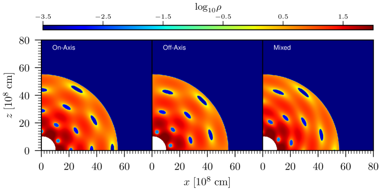
Figure 1: Initial rest-mass density distributions of the ejecta considered in our set of simulations. Note that the distributions are both inhomogeneous and anisotropic, with voids that are either “on-axis” (left panel), “ off-axis” (middle panel), or “mixed” (right panel) [see Eq. (2) for details].

In all of the cases considered, the constant $\rho_{0}$ is determine such that the total rest-mass in the ejecta, denoted by $M_{\rm ej}$, varies in the range $M_{\mathrm{ej}}/M_{\odot}\in[0.001,\,0.01]$, and corresponds to the range expected from BNS mergers (Rezzolla et al., 2010, 2011; Bauswein et al., 2013; Hotokezaka et al., 2013; Radice et al., 2016; Dietrich et al., 2017; Radice et al., 2018; Fujibayashi et al., 2023).

For a given choice of ejecta distribution and total rest-mass $M_{\rm ej}$, the jet will sweep on its path is a rest-mass column defined as

$$M_{\mathrm{path}}:=\int_{R_{\mathrm{in}}}^{R_{\rm{out}}}\int_{0}^{2\pi}\int_{0}^{\theta_{\mathrm{jet,i}}}\rho(r,\theta)r^{2}\,\sin\theta\,d\theta\,d\phi dr\,,$$ (5)

which does not change by more than $5\%$ across the various profiles and is at least $0.4\%$ of $M_{\mathrm{ej}}$.

By construction, the matter in the ejecta is all gravitationally unbound and the corresponding initial velocity profile is assumed to be isotropic and purely radial, increasing linearly with radius, i.e.,

$$\bm{v}_{\mathrm{ej}}=0.3\left(\dfrac{r}{r_{\mathrm{out}}}\right)\bm{e}_{r}\,,$$ (6)

where $\bm{e}_{r}$ is the unit-vector in the radial direction. Expression (6) leads to values that are close to those measured in numerical simulations (see, e.g.,  Baiotti & Rezzolla, 2017; Paschalidis, 2017; Shibata & Hotokezaka, 2019, for some reviews), and within the ranges inferred from the observations (see, e.g.,  Arcavi et al., 2017; Drout et al., 2017; Shappee et al., 2017; Pian et al., 2017; Kilpatrick et al., 2017; Kasliwal et al., 2017; Kasen et al., 2017; Evans et al., 2017; Smartt et al., 2017).

The jet is assumed to be launched by the “central engine” at the innermost radial shell and with an initial opening angle $\theta_{\mathrm{jet,i}}=0.1$. Its structure is assumed to be that of a “top-hat” jet, that is, with sharp cut-offs for all quantities at angles larger than the opening angle. For each simulation, we inject a jet with constant luminosity, $L_{\mathrm{jet}}$, using three different reference values $10^{49}\,\mathrm{erg/s}$, $5\times 10^{49}\,\mathrm{erg/s}$, and $10^{50}\,\mathrm{erg/s}$. The jet is injected in the grid for a duration of $t_{\mathrm{jet}}=1\,\mathrm{s}$ and has an initial Lorentz factor $\Gamma_{0}=10$. We set the asymptotic value of the Lorentz factor to $\Gamma_{\infty}=100$, which is translated to an initial specific enthalpy for the injected plasma of $h_{0}={\Gamma_{\infty}}/{\Gamma_{0}}$ since $h_{\infty}=1$. In practice, at every timestep and for the grid cells in the first radial slice within the jet opening angle we set

$$\Gamma=\Gamma_{0}\,,$$

$$\rho=\rho_{\mathrm{jet}}=2\pi\left(\dfrac{L_{\mathrm{jet}}}{\rho^{2}h_{0}\Gamma_{0}^{2}}\right)\left(\dfrac{1}{1-\cos(\theta_{\mathrm{jet}})}\right)\,,$$ (7)

$$p=p_{\mathrm{jet}}=\dfrac{1}{4}\rho_{\mathrm{jet}}(h_{0}-1)\,.$$

name	Lj.1.49.Me.001	Lj.1.49.Me.004	Lj.1.49.Me.010	Lj.5.49.Me.001	Lj.5.49.Me.004	Lj.5.49.Me.010	Lj.1.50.Me.001	Lj.1.50.Me.004	Lj.1.50.Me.010
$L_{\mathrm{jet}}$	$1\times 10^{49}$	$1\times 10^{49}$	$1\times 10^{49}$	$5\times 10^{49}$	$5\times 10^{49}$	$5\times 10^{49}$	$1\times 10^{50}$	$1\times 10^{50}$	$1\times 10^{50}$
$[{\rm erg/s}]$
$M_{\rm ej}$	$0.001$	$0.004$	$0.010$	$0.001$	$0.004$	$0.010$	$0.001$	$0.004$	$0.010$
$[M_{\odot}]$

Table 1: Properties of the various simulations performed in our analysis, each of which is marked by the corresponding jet luminosity $L_{\mathrm{jet}}$ and by the ejected mass $M_{\mathrm{ej}}$.

After a time $t=t_{\mathrm{jet}}$, which can be smaller or larger than the breakout time depending on its energy and mass of the ejecta, the central engine is not turned-off abruptly but following an exponential fall-off for a duration of $\tau_{\mathrm{rel}}=0.1\ t_{\mathrm{jet}}$, which, in turn, produces a sufficiently large decay of the asymptotic Lorentz factor. This smooth turning-off of the jet is implemented to avoid the generation of artificial shocks in the numerical domain, especially in the tail of the jet. After the transition time, we treat the inner radial boundary inside the jet-angle in the same way as we do for the ejected material. In other words, we set the rest-mass density to follow a power-law in time with exponent $-6$. A summary of the physical properties of the 27 different simulations carried out in our investigations can be found in Table 1.

Finally, our 2D grid has a number of base cells in the radial and polar direction given by $N_{r}\times N_{\theta}=1120\times 576$ and we employ three refinement levels, thus reaching a peak effective resolution of $N_{r}\times N_{\theta}=8960\times 4608$. This is a rather high resolution that provides us with sufficiently detailed information about the dynamics of the jet during its propagation and breakout. Furthermore, a discussion of the consistency and robustness of our results when considering different numerical resolutions can be found in Appendix A.

2.2 Large-scale jet structure and afterglow emission

In order to determine the astronomical observables that would allow us to probe the jet-ejecta interaction, we calculate the afterglow radiation produced as a result of the jet morphology computed in the various simulations. To this scope, we first need to compute the angular structure in total jet energy ${\rm d}E_{\rm jet}/{\rm d}\Omega(\theta)$ and in Lorentz factor $\Gamma_{\infty}(\theta)$, which are extracted from the simulation, at a time of $t=2.25\,\mathrm{s}$ after launching of the jet. To compute the energy density $e$ in the inertial frame for a perfect fluid moving with Lorentz factor $\Gamma$ we can make use of the fact that it possesses a conserved quantity, namely, the Bernoulli constant given by (see, e.g.,  Rezzolla & Zanotti, 2013, Secs. 3.6.2 and 11.9.2)

$$hu_{t}=\left(\frac{e+p}{\rho}\right)\Gamma=\left(1+4\frac{p}{\rho}\right)\Gamma={\rm const.}\,.$$ (8)

Hence, for a perfect fluid obeying an ideal-fluid equation of state with adiabatic index $\gamma=4/3$, expression (8) can be inverted to obtain the energy density of the fluid in the inertial frame

$$e(r,\theta)=\rho\bigg{(}1+4\ \dfrac{p}{\rho}\bigg{)}\Gamma^{2}-p\,.$$ (9)

To obtain the distribution of jet energy per solid angle at latitude $\theta$, we integrate Eq. (9) over the radial direction:

$$\frac{{\rm d}E_{\rm jet}}{{\rm d}\Omega}(\theta):=\int^{r_{\mathrm{out}}}_{r_{\mathrm{ej,front}}}e(r,\theta)\,r^{2}dr\,,$$ (10)

which we will refer to as the “$E$-structure”, where $r_{\mathrm{ej,front}}$ is the ejecta front, a choice made to avoid including plasma from unshocked ejecta in the jet structure and is calculated by :

$$r_{\mathrm{ej,front}}>R_{\rm out}+v_{\mathrm{ej,max}}\,t_{\rm ex}\,,$$ (11)

where we set $v_{\mathrm{ej,max}}=0.6$ [Eq. (6)] and $t_{\rm ex}=2.25\,{\rm s}$ is the extraction time of the jet structure in the simulation domain (see also Sec. 3.3). The choice of the definition of the energy structure as the energy per unit volume is guided by the fact that this function is constant in a top-hat jet, or generally in an isotropic expansion, and because it is usually considered in prior numerical work and analytical work. In this integral, the choice of bounds in radius $r_{1}$ and $r_{2}$ is done to consider only relativistic material in the domain, as explained below.

We define the jet structure in Lorentz factor via the asymptotic Lorentz factor $\Gamma_{\infty}$, which can be easily calculated using again the Bernoulli constant to obtain:

$$h_{\rm{\infty}}\Gamma_{\rm{\infty}}=\Gamma_{\rm{\infty}}=\Gamma\bigg{(}1+4\ \dfrac{p}{\rho}\bigg{)}\,,$$ (12)

that is, the Lorentz factor that the material would reach if all its internal energy were converted to kinetic energy. Then, we determine the average asymptotic Lorentz factor in the solid angle around latitude $\theta$

$$\Gamma_{\infty}(\theta):=\frac{\int^{r_{\mathrm{out}}}_{r_{\mathrm{ej,front}}}\Gamma_{\infty}(r,\theta)r^{2}dr}{\int^{r_{\mathrm{out}}}_{r_{\mathrm{ej,front}}}r^{2}dr}\,,$$ (13)

that we refer to as the “$\Gamma$-structure”.

We note that when performing the volume integrals to determine both the $E$- and $\Gamma$-structures we need to avoid taking into account plasma that is not relativistic a simply part of the moving ejecta. To this scope, we define different criteria to examine whether a cell should be excluded or not from the domain. In essence, they consist of cut-offs in asymptotic velocity, which are considered to only include in the relativistic jet material with Lorentz-factor high enough to accelerate a population of non-thermal particles in the forward shock susceptible to produce synchrotron radiation (Sironi et al., 2013). (see Sec. 3.1 for more details on these Lorentz-factor cutoffs and the robustness of our results with respect to different choices).

The procedure outlined above allows us to determine the structure of the jet, i.e., the dependence of the Lorentz factor and energy of the outflow on the polar angle with respect to the jet axis. Once emerged from the jet, the outflow will then decelerate by colliding with the interstellar medium leading to the afterglow emission. Given the likely achromaticity of afterglows of jets viewed off axis, we restrict our study in the emission in the radio band (Duque et al., 2019; Beniamini et al., 2020a) and model the afterglow light-curves in the radio by following the procedure described by Granot et al. (2002) and Gill & Granot (2018), which we briefly review below.

First, we assume that each angular slice of the relativistic jet evolves independently of the others; this amounts to ignoring the lateral spreading (i.e., considering $v^{\theta}=0=v^{\phi}$) and tends to an over-estimation of ${\rm d}E_{\rm jet}/{\rm d}\Omega$ and $\Gamma_{\infty}$. The interaction of the jet with the ambient medium obviously leads to what is normally referred to as the “forward” shock and which is responsible for dominant part of the emission (see Granot & Sari 2002 for the validity of this assumption). The dynamics of the forward shock proceeds through two different phases in time. First, during the so-called “coasting phase”, the shock front propagates with a constant Lorentz factor $\Gamma(r)=\Gamma_{0}$ until a deceleration radius

$$R_{d}\approx 1.3\times 10^{17}\bar{n}^{-1/3}\left(\frac{E}{10^{53}\,{\rm erg}}\right)^{1/3}\left(\frac{\Gamma_{0}}{100}\right)^{-2/3}\mathrm{cm}\,,$$ (14)

for uniform circum-burst medium, where $\bar{n}$ is the number density of the ambient medium the jet penetrates after the breakout. We determine the deceleration radius and subsequent deceleration dynamics for all the angular slices according to the $E$- and $\Gamma$-structure as described previously.

Following the case of GW170817 and in line with the low densities expected in media around BNS mergers, we adopted $\bar{n}=3\times 10^{-3}\,{\rm cm}^{-3}$ with a uniform circum-burst medium for all our afterglow calculations. Once sufficient material has been swept up and energised in the forward shock, the jet decelerates significantly, such that, for any polar angle $\theta$, the Lorentz factor evolution with radius follows  (Panaitescu & Kumar, 2000):

$$\Gamma(\xi)=\dfrac{\Gamma_{0}+1}{2}\xi^{s-3}\bigg{[}\sqrt{1+\dfrac{4\Gamma_{0}}{\Gamma_{0}+1}\xi^{3-s}+\left(\dfrac{2\xi^{3-s}}{\Gamma_{0}+1}\right)^{2}}-1\bigg{]}\,,$$ (15)

where $\xi:={r}/{R_{d}}$. After the coasting phase, the following relation is recovered for the radial dependence of the Lorentz factor of the forward shock: $\Gamma(\xi)\propto\xi^{-(3-s)/2}$ (Blandford & McKee, 1976), where $s$ is the power-law index of the circum-burst medium, equal to $s=0$ in our case of a uniform medium. This corresponds to the “deceleration phase”. To capture the entire evolution of the afterglow light-curve, we consider $\xi$ in the range from $r=0$ up to the Newtonian radius $R_{{}_{\rm N}}:=\Gamma_{0}^{2/(3-s)}R_{d}$, where the jet becomes non-relativistic.

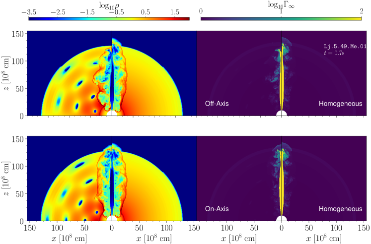
Figure 2: Comparison of jet-breakout dynamics for the case Lj.5.49.Me.010 (i.e., $L_{\mathrm{jet}}=5\times 10^{49}\,{\rm erg/s}$ and $M_{\mathrm{ej}}=0.10\,M_{\odot}$). The panels in the left column show the rest-mass density, while those in the right column report the distributions of the Lorentz factor. To highlight the contrast among different distributions, the left part of each panel reports the anisotropic distribution of rest-mass density (“off-axis” in the top row and “on-axis” in the bottom row), while the right part the dynamics across a homogeneous distribution. All panels refer to a time $t=0.7\,{\rm s}$ since the launch of the jet.

For a given observation angle $\theta_{\mathrm{obs}}$ and a given angular slice of the jet $\theta$, we calculate the afterglow flux assuming synchrotron emission from the forward shock formed as the relativistic jet decelerates (Nakar et al., 2002). According to the semi-analytical solution for the deceleration of the jet where the forward shock forms, the forward shock has a comoving internal energy density of ${u^{\prime}}=(\Gamma-1){n^{\prime}}m_{p}$, where ${n^{\prime}}(r)\approx 4\Gamma(r)\bar{n}$ is the comoving particle number density in the shock and $\Gamma(r)$ is the Lorentz factor of the forward shock once it has reached radius $r$ (Blandford & McKee, 1976).

The fraction of this energy that is deposited to relativistic electrons is denoted as $\epsilon_{e}$ and essentially determines the mean Lorentz factor of these electrons in the frame comoving with the shock. We assume that the electrons obey a power-law distribution ${n^{\prime}}(\gamma_{e})\propto\gamma_{e}^{-q}$, as it is expected from acceleration processes, and shown by particle-in-cell simulations (see, e.g.,  Sironi & Spitkovsky, 2011; Meringolo et al., 2023). The power law index $q\ (>2)$ of the non-thermal electrons in the afterglow emission is chosen to be $q=2.2$, as suggested by the ratio of afterglow fluxes in various bands in GW170817 (e.g. The LIGO Scientific Collaboration et al., 2017) and other SGRB afterglows (Cenko et al., 2011). Furthermore, in the shocked material, a small-scale turbulent magnetic field is produced and we assume that a fraction $\epsilon_{{}_{B}}$ of the comoving internal energy is transformed into magnetic energy in the shocked matter to power the synchrotron emission, such that the magnetic-field strength is $B^{2}=8\pi\epsilon_{{}_{B}}u^{\prime}$ (Granot et al., 1999). Hereafter, and unless stated otherwise, we set $\epsilon_{e}=0.112$ and $\epsilon_{{}_{B}}=10^{-3}$; these values are in agreement with the posterior bounds given by Ghirlanda et al. (2019).

Once the distribution of non-thermal electrons and the magnetic-field strength is set, we can determine the comoving spectral luminosity $L^{\prime}_{\nu^{\prime}}$ due to the synchrotron emission for each angular slice of the jet over the region of deceleration. We use the expression for $L^{\prime}_{\nu^{\prime}}$ from Gill & Granot (2018), equations 13 and following. This expression covers all the segments of the standard synchrotron spectrum as a function of the basic physical quantities of the shock that we previously presented, namely, $n^{\prime}$, $u^{\prime}$, $\epsilon_{e}$, $\epsilon_{{}_{B}}$, and $q$.

Finally, we calculate the total flux from the jet at radio frequency $\nu=3\,{\rm GHz}$ for a distant observer at viewing angle $\theta_{\rm obs}$ and observing time $t$ by integrating the comoving spectral luminosity over the jet structure on equal-arrival-time surfaces, as in Gill & Granot (2018). In the end, the jet-structure integral is written as an integration over angles

$$F_{\nu}(t)=\dfrac{1}{16\pi^{2}d_{{}_{L}}^{2}}\int\delta_{{}_{D}}^{3}\,\,{L^{\prime}}_{{\nu}^{\prime}}\,\,d\cos\theta\,d\phi\,,$$ (16)

where $\delta_{{}_{D}}:=[\Gamma(1-v_{\rm jet}\cos\chi)]^{-1}$ is the so-called Doppler factor ($v_{\rm jet}$ is the jet velocity), so that the two frequencies are related through $\nu=\delta_{{}_{D}}\nu^{\prime}$, and $\chi$ is the angle between the line of sight and the angular slice at $(\theta,\phi)$ at hand in the integration over the structure. For definiteness, we chose a luminosity distance of $d_{{}_{L}}=40\,{\rm Mpc}$, small enough to allow us to ignore redshift corrections. The choice of this distance is not very important, as we are mostly interested in the morphology of the afterglow light-curves. Given the small external density we consider ($\bar{n}=3\times 10^{-3}\,{\rm cm}^{-3}$), the effects of synchrotron self-absorption can be neglected (Duque et al., 2020).

3 Results

3.1 Jet propagation and breakout

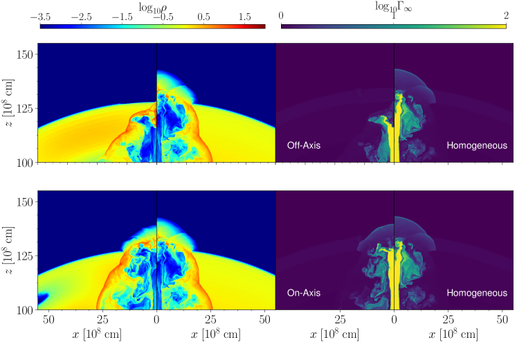
Figure 3: The same as in Fig. 2 but on a scale highlighting the breakout region.

We start by studying the effect of the anisotropies in the rest-mass density distribution on the propagation of the jet in the ejecta. Figure 2 shows a snapshot of the jet-ejecta evolution at the time of the jet breakout for different ejecta density profiles from the Lj.5.49.Me.010 runs (see Table 1). In particular, Fig. 2 reports in its left panel the rest-mass density distribution, while on the right panel the distribution of the Lorentz factor (Figure 3 reports the same quantities as Fig. 2 but on a scale that highlights the breakout region). For each panel, in addition, the left part refers to a simulation with an anisotropic and inhomogeneous distribution (“off-axis” on the top row and “on-axis” on the bottom row), while the right part provides the evolution in the reference case of an isotropic but inhomogeneous distribution.

When comparing the different parts of the figure, it becomes apparent that the jet propagation is only mildly affected by the presence of the anisotropic perturbations in the ejecta distribution. In turn, the breakout time and energies of the jet at breakout are rather similar among all cases considered, including the homogeneous one (see discussion below for details). At the same time, differences do appear in the morphology of the matter that interacts with the jet and that is set in turbulent motion by the propagation of the jet. This is more evident in the case of the “off-axis” perturbations, which lead to a significant lateral expansion of the jet as it encounters regions in the ejecta with significantly smaller densities. However, differences are present also for the “on-axis” perturbations but, interestingly, these mostly cancel out. In particular, the acceleration following the interaction with an underdense region along the jet direction are compensated by the deceleration when the jet encounters an overdense region. As a result, the jet breaks-out almost at the same time as in the case of a propagation across an isotropic ejecta distribution (compare the left and right parts of the bottom-left panel of Figs. 2 and 3).

The qualitative description offered by Figs. 2 and 3 can be complemented by a more quantitative description summarised in Fig. 4, which reports, in the left panel, the jet breakout time $t_{\rm jet,bo}$, and in the middle panel, the opening angle of the structured jet $\theta_{\rm jet}$. More specifically, we define $t_{\rm jet,bo}$ as the time when the material shocked by the propagating shock first overtakes the radially expanding ejected matter.

As we will show in more detail in Fig. 7, the Lorentz factor experiences a steep decrease outside of inner region (core) that allows us to robustly define the angular size of the ultra-relativistic core of the jet, denoted by $\theta_{\mathrm{jet}}$ and defined as the smallest angle for which $\Gamma_{\infty}<10$. We extract this data from the profiles presented in Fig. 7. We plot this angle on the middle panel of Fig. 4. We find that this angle varies by at most $1.5\,\mathrm{deg}$ when changing the pattern of the perturbations in the ejecta density and, in cases where the ejecta mass is low, this variation is much less than $10\%$. This suggests that, under the condition of a successful jet breakout, the jet core is largely unaffected by the ejecta profile.

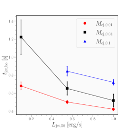
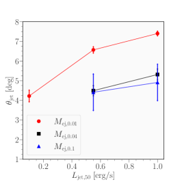
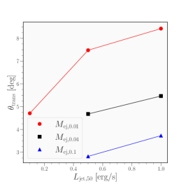
Figure 4: Left panel: Jet-breakout time from the ejecta as a function of the jet luminosity (horizontal axis) and of the mass in the ejecta (different coloured lines and symbols). Middle panel: The same as in the left panel but for the jet opening angle. Right panel: The same as in the left panel but for the transition angle from the steep to the shallow segment in the energy polar structure of the jet [see Eq. (19) for details]. In all panels, the vertical bars mark the variation that comes from the different rest-mass density distributions.

The jet break-out and core opening angles reported in Fig. 4 are shown as function of the three luminosities assumed for the jet (horizontal axis) and of the rest-mass density contained in the ejected material (black, red and blue symbols, respectively). Furthermore, the variance shown with vertical lines across the solid symbols reflects the different geometry of the anisotropies (i.e., “off-axis”, “on-axis”, or “mixed”) and indicates one of the most important results of our work, namely that the impact of the geometric anisotropies on jet break-out and jet core properties is not very large and that these jet properties are mainly set by the energy in the jet and by the mass in the ejecta.

Starting from the left in Fig. 4, it is apparent that the breakout time decreases as the energy of the jet is increased, but also that it increases as the ejected matter is more massive. The interpretation of this behaviour is straightforward: the jet travel-time across the ejecta will depend on its energy and on the matter resistance it will encounter, so that the most massive ejecta may actually prevent the breakout of the weakest jet, while the most powerful jet will cross the least massive ejecta in only $0.4\,{\rm s}$. At the same time, for a given mass of the ejecta, the breakout time can even double between the least and the most powerful jets. Interestingly, the jet with $L_{\rm jet,50}=0.10\,{\rm erg/s}$ (simulation Lj.1.49.Me.010) is indeed chocked when going across the massive ejecta with $M_{\rm ej}=0.010\,M_{\odot}$. This behavior is in agreement with the predictions for the “early-breakout” criterion of (Duffell et al., 2018) [Eq. (20) there] but in tension with the “late-breakout” criterion, which instead predicts a successful jet; as pointed out by Gottlieb & Nakar (2022), this tension may be due to the way that the jet is being “turned off”. An abrupt shutdown of a jet, or an extended transition phase will have an impact on the cases of “late-breakout”. We also note that the variability of the break-out time induced by the anisotropies is larger for the intermediate mass ejecta (see, e.g., Fig. 4). This behaviour, could be due to a number of potential effects but we conjecture it is the result of the fact that in the case of intermediate mass ejecta the system is intrinsically closer to a near-cancellation of effects, which is not present if the mass of the ejecta is very large or very small. Under these conditions, small fluctuations, even numerical in nature, can lead to large variations in quantities such as the break-out time or the jet opening angle.

Also, the 2D nature of our simulations, inevitably implies the presence of the so-called “plug-instability” (Zhang et al., 2004; Mizuta & Ioka, 2013; López-Cámara et al., 2013), which is not really an instability but rather the artificial piling up of matter ahead of the propagating jet (in 3D this matter has more opportunities to move in the direction orthogonal to that of the jet) and hence affects in part the dynamics of the jet propagation. Fully three-dimensional simulations have shown that the plug-instability tends to over-estimate the breakout time by introducing a systematic bias in the breakout time (see Appendix of Urrutia et al., 2021), which is likely to affect also our results. However, we expect that the basic phenomenological trend of the breakout time as a function of $L_{\rm jet}$ and $M_{\rm ej}$ portrayed in the left panel of Fig. 4 to be robust and hence to be present also in fully 3D simulations.

The physically intuitive behaviour of the breakout time is shared also by the jet opening angles $\theta_{\rm jet}$, shown in the middle panel of Fig. 4, respectively. In essence, what these panels highlight is that this angle increases as the energy of the jet is increased and decreases as the mass in the ejecta is increased. Once again, this is not surprising as it is natural to expect that more powerful jets will deposit systematically larger amounts of energy in the ejecta, leading to larger opening angles at the breakout. Conversely, a larger ejecta mass will exert more pressure on the propagating jet and close the core angle before breakout. Less obvious is that this behaviour should be essentially linear in $L_{\rm jet}$, while it is clearly nonlinear in terms of $M_{\rm ej}$ (see Fig. 4).

3.2 Cocoon evolution

As mentioned in the previous section, the propagation of the jet within the ejected envelope leads to a turbulent shear layer that is normally referred to as the “cocoon” for its peculiar shape. At the breakout time, Figs. 2 and 3 illustrate the detailed morphology of the cocoon, which can be readily identified by the steep gradient in density. More precisely, we distinguish the matter in the cocoon from the jet material by following the conditions proposed by Hamidani & Ioka (2023), that is, we mark as filled with cocoon-matter cells for which the following conditions are met: $\Gamma_{\infty}\leq 10$, $\Gamma<5$, and $\lvert v_{\theta}\rvert>0$, where the last criterion is imposed to avoid the mis-identification of ejected material or interstellar medium (for which $\lvert v_{\theta}\rvert=0$) with the matter in the cocoon. Clearly, Fig. 2 shows that the cocoon varies at different vertical heights and hence it changes during the evolution. More importantly, it is easy to realise that the different geometric properties of the ejected material do have an impact on the morphology of the cocoon.

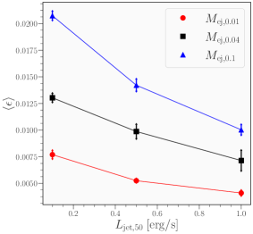
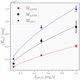
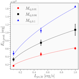
Figure 5: The same as in Fig. 4 but for the diagnostics of the thermal energy in the cocoon during the jet evolution. In particular, shown are: the average efficiency of jet-cocoon energy transfer [Eq. (17), left panel], the time-averaged thermal energy of the cocoon up until the jet breakout (middle panel), and the peak thermal energy of the cocoon during the jet evolution (right panel). In the last two panels, the dashed lines indicate the square-root fit with the jet luminosity.

During its propagation across the ejected material, the jet will deposit a part of its kinetic energy increasing the internal energy of the ejecta $E_{\mathrm{th}}$. Since the $L_{\rm jet}$ is the source of energy, we can define the efficiency $\epsilon$ with which the jet energy is converted into the thermal energy of the cocoon as

$$\frac{dE_{\mathrm{th}}}{dt}=:\epsilon(t)L_{\mathrm{jet}}\simeq\langle\epsilon\rangle L_{\mathrm{jet}}\simeq\frac{\langle E_{\mathrm{th}}\rangle}{t_{\rm jet,bo}}\,,$$ (17)

where $\langle E_{\mathrm{th}}\rangle$ is the time-averaged thermal energy deposited in the ejecta from the start and up to the breakout time $t_{\rm jet,bo}$. The unknown efficiency $\epsilon$ (and its time-averaged counterpart $\langle\epsilon\rangle$) takes into account the work done both on the jet head surface via the forward shock and that done in generating a lateral expansion of the cocoon [the (kinetic) energy in the turbulent motion in the cocoon is not included in expression (17)]. Clearly, the value of such an efficiency will depend on the properties of the ejected material and, in our setup, on the properties of the anisotropies introduced. Using our simulations and the measurements of $\langle E_{\mathrm{th}}\rangle$, we have estimated the average efficiency $\langle\epsilon\rangle$ and summarised the results in the left panel of Fig. 5 for the configurations considered. It is then interesting to note that the time-averaged efficiency $\langle\epsilon\rangle$ decreases linearly with increasing energy in the jet and increases with the mass in the ejecta. Stated differently, more energetic jets are less efficient in converting the kinetic energy into thermal energy, especially if the ejecta are not very massive. This behaviour is rather natural and indeed one would expect a vanishing efficiency for extremely tenuous ejecta and very energetic jets, which would propagate in them essentially ballistically. Note also how the efficiency is also upper-limited by a value of about $1.5\%$, which corresponds to the configuration Lj.1.49.Me.004 that we will later-on see, is that of a marginally successful breakout.

Considering the amount of energy that is needed to explain the early blue component of the kilonova of GW170817, Duffell et al. (2018) concluded that the exchange of thermal energy in the jet-cocoon system is subdominant. To validate this conclusion, we report in Fig. 5 the time-averaged thermal energy deposited in the ejecta $\langle E_{\mathrm{th}}\rangle$ (middle panel) and the peak thermal energy $E_{\rm th,peak}$ (right panel), that is, the largest value of $E_{\rm th}$ recorded for the cocoon during the jet propagation through the ejecta, as a function of the energy in the jet and mass in the ejecta. The behaviour of the two quantities is similar even though they really refer to distinct quantities as $\langle E_{\mathrm{th}}\rangle$ contains information on the overall “heating” of the ejecta, while $E_{\rm th,peak}$ is mostly indicative of observational properties, especially when the observations are performed with sensitivity-limited instruments. Overall, both panels reveal that the energy deposited in the ejecta to produce the cocoon increases with the mass of the ejecta and the luminosity of the jet, and scales like the square root of the latter, as also anticipated by (Duffell et al., 2018). This is shown by the dashed lines that show a fitting function with power-law index equal to $1/2$.

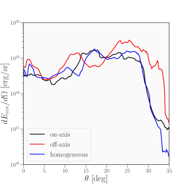
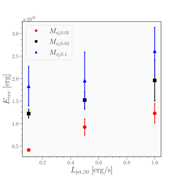
Figure 6: Left panel: polar distribution of the energy in the cocoon for the model Lj.1.50.Me.001 and different anisotropies (different coloured lines). Right panel: total energy in the untrapped cocoon shown as a function of the jet luminosity and masses in the ejecta (different coloured symbols). Also in this case, the vertical bars mark the variation that comes from the different density profiles.

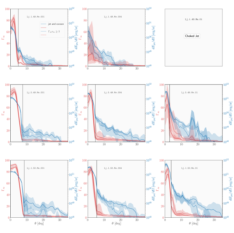
Figure 7: Large-scale polar structures at $t=2.25\,\mathrm{s}$ of the nine jets simulated and shown in terms of the total energy (blue lines) and of the Lorentz factor (red lines). Each panel is marked by the name of the corresponding case reported in Table 1 and the top-right panel refers to the case when the jet is unable to break out from the ejecta (i.e., “chocked jet”). Solid lines refer to polar structures computed considering the entire plasma outside the ejecta (i.e., “jet and cocoon”), while the dashed lines refer to structures after imposing a a velocity cut (i.e., $u_{\infty}>3$). In all cases, the blue/red shaded areas report the variance due to the different types of anisotropy in the ejecta. Shown with a black solid vertical line is the transition angle $\theta_{\rm trans}$ (cf., Fig. 4).

In addition, note how the variance introduced by the different anisotropies plays a very modest role in determining the amount of energy deposited and that the impact is larger for the most energetic jets. Still within the context of the GW170817 event, early emission from the cocoon has been studied (see, e.g.,  Nakar & Piran, 2017; Gottlieb et al., 2018) and associated with early observations of an electromagnetic counterpart. Because of the delay of about 10 hours in the localisation of the source, the cocoon contribution to the emission was likely unobserved. Nonetheless, Piro & Kollmeier (2018) claimed the detection of prompt emission in association with the GW170817 event. More recently, Hamidani & Ioka (2023) have built an analytical model to examine the differences between jets produced in collapsars and in SGRBs environment, the main difference being the static or homologously expanding ejecta. In this way, they found that at most $10\%$ of the cocoon mass can escape from the ejecta, and therefore only a small portion of the cocoon energy can escape and contribute to the early emission. Indeed, as long as the cocoon is buried in the ejecta and these are optically thick, it cannot be observed. However, since the ejecta are expanding and cooling, the optical depth will reach, on a timescale of about one day, values below unity revealing the cocoon. Hence, it is important to compare the timescale for the emergence of the emission from the cocoon with the other timescales, namely $t_{\rm jet,bo}$ or the delay between breakout and the $\gamma$-ray emission.

In view of these considerations, and given the wealth of information provided by our simulations, it is interesting to assess what impact the anisotropies in the ejecta have on the amount of energy in the cocoon that is trapped in the ejecta. To this scope, and since all of the ejecta is already unbound, we need to mark the part of the “untrapped” cocoon as the material of the cocoon that is moving faster than the ejecta; since the velocity in the ejecta increases linearly with radius [Eq. (6)] and reaches a maximum of $v_{\mathrm{ej,edge}}$ at the forward edge, matter in the untrapped cocoon should satisfy the additional condition

$$v_{\mathrm{coc},\infty}\geq v_{\mathrm{ej,edge}}\,,$$ (18)

where the terminal velocity is calculated as $v_{\mathrm{coc},\infty}=h_{\rm coc}v_{\mathrm{coc}}$. For this matter, we then measure the corresponding energy polar distribution ${\rm d}E_{\rm coc}/{\rm d}\Omega(\theta)$ of the untrapped cocoon in analogy with what was done for the energy in the jet [Eq. (10)]. Also, we compute the total energy in the untrapped cocoon $E_{\rm coc}$ as the volume integral of the energy density for matter satisfying the condition (18).

The results are summarised in Fig. 6, whose left panel reports the angular distribution of the energy of the “untrapped” cocoon for three different cases of ejecta, namely, “on-axis”, “off-axis” and “homogeneous”. Note how the polar distribution in the cocoon energy is rather similar in the case of the homogeneous and on-axis ejecta, while it differs in the case of off-axis anisotropies, where more energy is concentrated at higher latitudes. While this may appear surprising, it reflects the analogy already remarked between the propagation across homogeneous and on-axis perturbations, where the sequence of over- and under-densities along the jet path compensate and cancel out, hence giving a very similar cocoon and breakout time as in the homogeneous case (cf., Figs. 2 and 3). The right panel of Fig. 6, on the other hand, shows $E_{\rm coc}$ as a function of the two main parameters of our setup, i.e., $L_{\rm jet}$ and $M_{\rm ej}$, and the corresponding variance with the initial anisotropies of the ejecta shown again as vertical bars. Rather unsurprisingly, the energy in the cocoon that is able to escape grows with both the energy in the jet and with the mass in the ejecta. In turn, this implies that even if parts of the ejecta are energised more significantly because of their lower density, follow-up interactions with a denser medium do not produce significant changes on the overall dynamics of the cocoon.

3.3 Large-scale jet polar structure

Using the procedure described in Sec. 2.2, we next discuss the large-scale polar structure of the jet. For the sake of brevity, we introduce the short-hand notation $E_{\Omega}(\theta)$ for the distribution of jet energy per unit solid angle ${\rm d}E_{\rm jet}/{\rm d}\Omega(\theta)$. In particular, for all of the runs performed Fig. 7 reports the polar dependence of the jet Lorentz factor $\Gamma_{\infty}(\theta)$ (red curves) and energy $E_{\Omega}(\theta)$ (blue curves). More specifically, for each pair of $L_{\mathrm{jet}},M_{\rm ej}$, the solid lines in the various panels report respectively the average $E_{\Omega}(\theta)$ and $\Gamma_{\infty}(\theta)$ across the three perturbation distributions (“on-axis”, “off-axis”, and “mixed”); the shaded areas, on the other hand, span the ranges $\Delta E_{\Omega}(\theta)$ and $\Delta\Gamma_{\infty}(\theta)$ among the three distributions, as due to the different choices in profiles of the density in the inhomogeneous ejecta. Note that in each panel of Fig. 7 we present the angular profiles assuming two different cuts in velocity when computing the energy and Lorentz-factor integrals [Eqs. (10) and (13)]. The first cut (solid lines), aims at representing both the cocoon and the jet and corresponds to matter with a velocity $v_{\infty}>0.3$. The second cut (dotted line), shows instead only the mildly-relativistic to relativistic outflow and corresponding to a cut $\Gamma_{\infty}v_{\infty}\geq 3$. This cut is meant to refer to material that is expected to contribute the most to the afterglow radiation through the forward shock. Indeed, below this velocity, the efficiency of the forward shock in accelerating the population of non-thermal electrons necessary for the synchrotron emission from the shocked region, is considerably smaller (see, e.g.,  Morlino & Caprioli, 2012; Crumley et al., 2019).

Figure 7 reveals that, except for the particular case of Lj.1.49.Me.004, which we discuss separately later, all the simulations show a similar behaviour for the polar structure of the jet. In particular, the polar profiles of the Lorentz factor consistently show a “core” with large (i.e., $\Gamma_{\infty}\sim 60-90$) and near-constant values of $\Gamma_{\infty}$ within an angle of $\theta\approx 5\,\mathrm{deg}$, which is closely related to the initial jet opening angle $\theta_{\rm jet,i}$. The Lorentz factor then exhibits a sharp decrease down to $\Gamma_{\infty}\lesssim 10$ for $\theta\gtrsim 7\,{\rm deg}$; this sharp decrease, which we have indicated with $\theta_{\rm jet}$ in Fig. 4, can be well described by a power-law dependence $\Gamma_{\infty}(\theta)\propto\theta^{-\beta}$ with $\beta>7$ for all configurations considered.

Similarly, the polar profiles of the energy also consistently exhibit a core region, with an energy level that is largely independent of the choice of the perturbation pattern in the ejecta. Outside of this core, the energy polar structures then present a decreasing segment where, just like for the Lorentz factor, the profiles are largely independent of the density anisotropies in the ejecta. However, in contrast to the $\Gamma$-structure, the $E$-structure does not have a sharp fall-off for $\theta\gtrsim\theta_{\rm jet,i}$, but a much slower decay ranging from a flat distribution (e.g., Lj.5.49.Me.001) to slopes with a power-law index $\beta\sim 3$ (e.g., Lj.5.49.Me.004) up to large latitudes up to $\theta\approx 25\,\mathrm{deg}$. This region of slower decay contains a significant reservoir of energy and, remarkably does depend on the actual pattern of anisotropies in the ejecta and, as we will show below, strongly impacts the afterglow emission, most notably at early times.

To discuss this original feature of the $E$-structures, we introduce the angle $\theta_{\rm trans}$, defined as the transition angle from the steep segment to the shallow segment in the energy structure of the jet. To capture this transition from the ejecta-pattern-independent to the pattern-dependent segment of the structure we define $\theta_{\rm trans}$ as the angle marking a relative difference larger than $50\%$, between the average structure and the structure range i.e.,

$$\theta_{\rm trans}={\rm min}\left\{\theta\left|\frac{\Delta E_{\Omega}(\theta)}{E_{\Omega}(\theta)}>50\%\right.\right\}\,,$$ (19)

which depends on the injected jet energy and on the mass of the ejecta. This angle is reported as a vertical black solid for all cases shown in Fig. 7. In addition, in the right panel of Fig. 4, we report $\theta_{\rm trans}$ as a function of $L_{\rm jet}$ for different values of $M_{\rm ej}$. We find that, analogously to $\theta_{\rm jet}$, $\theta_{\rm trans}$ increases with $L_{\rm jet}$ and decreases with $M_{\rm ej}$, underlining the larger or lesser capacity for the jet to expand without being affected by the anisotropies in the ejecta.

Before concluding this section, we concentrate on the case of Lj.1.49.Me.004, which, as already anticipated, deviates from this general trend. While this configuration does produce a large-scale jet with a significant Lorentz factor in the core (on average in the core, $\Gamma_{\infty}\gtrsim 30$), there are some density anisotropies in the ejecta that do not lead to an ultra-relativistic jet emerging on a large scale (indeed $\Gamma_{\infty}\lesssim 10$ in the core for a “off-axis” anisotropic distribution). In addition, the average Lorentz factor in the core is significantly lower than that of the injected jet, and is very low with respect to constraints on SGRB jets. Considering that a similar configuration with a more massive set of ejecta, i.e., Lj.1.49.Me.010, does not lead to a successful breakout but to a chocked jet, we interpret the phenomenology associated with Lj.1.49.Me.004 as to that of a marginally successful breakout. In this configuration, therefore, the energy injected is only marginally sufficient to produce a successful motion across the ejecta that, when slightly more massive, are instead capable of preventing the progression of the jet. We can use these two cases, namely Lj.1.49.Me.004 and Lj.1.49.Me.010, to set a minimum threshold for the “critical efficiency” necessary for a successful breakout given an ejecta mass and a jet propagating at a given luminosity. In particular, using the data for Lj.1.49.Me.010 we determine such an efficiency to be

$$\eta_{\rm crit}:=\left(\frac{L_{\rm jet}}{10^{50}\,{\rm erg/s}}\right)\left(\frac{t_{\rm jet,bo}}{1\,{\rm s}}\right)\left(\frac{M_{\rm ej}}{10^{-3}\,M_{\odot}}\right)^{-1}\gtrsim 0.03\,.$$ (20)

The robustness of this result is provided by the fact that all configurations have efficiencies larger than $\eta_{\rm crit}$ and the same behaviour discussed so far is measured when using other extraction times, e.g., $t_{\rm ex}=2.0,\,2.2\,{\rm s}$, or when varying the threshold for our velocity cut, e.g., $\Gamma_{\infty}v_{\infty}=2.0,\,2.5$. Finally, the estimate in Eq. (20) is in reasonable agreement with similar but distinct estimates (Duffell et al., 2018).

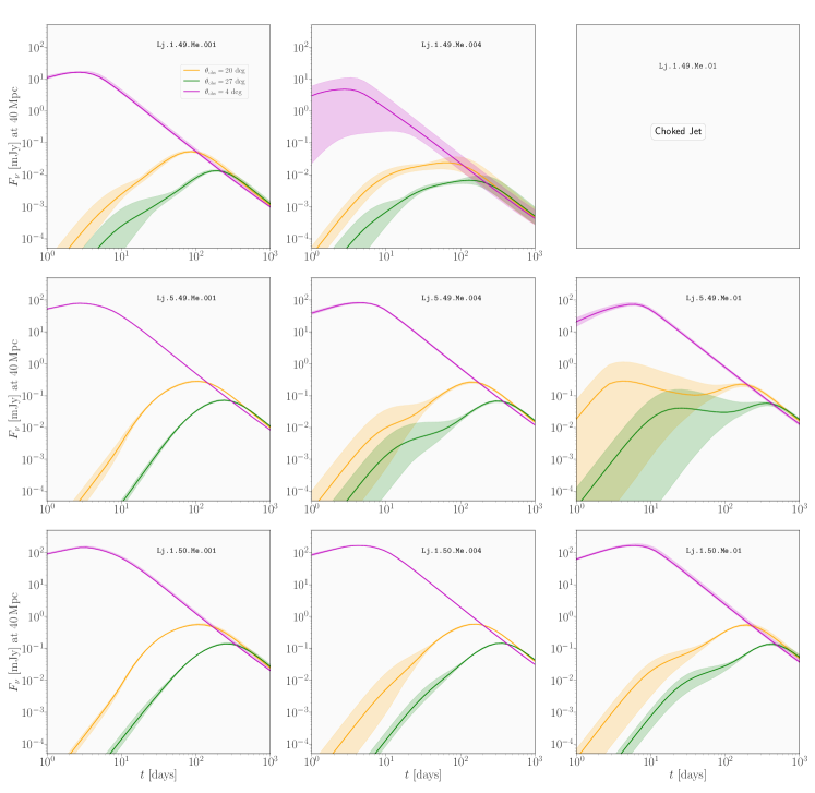
Figure 8: Afterglow emission of the nine jets simulated; each panel is marked by the name of the corresponding case reported in Table 1 and the top-right panel refers to the chocked jet. For each panel, the different lines refer to the different viewing angles of the observers and the corresponding coloured shaded areas report the variance due to the different types of anisotropy in the ejecta. Note that in the case of model Lj.1.49.Me.004 the light-curve is double peaked as a result of complex distribution of the jet energy in the shallow segment (see main text for a discussion).

3.4 Afterglow predictions and observations

Starting from the jet structures shown in Fig. 7, we can produce the radio afterglow light-curves emission following the procedure discussed in Sec. 2.2. These light-curves are reported in Fig. 8 for three different viewing angles $\theta_{\rm obs}=4$ (magenta lines), $20$ (orange lines) and $27\,{\rm deg}$ (green lines), representing, respectively lines of sight that are either “on-axis” (magenta line) or “off-axis” (orange and green lines); the shading around these lines follows the convention already employed in Fig. 7, namely, marking the variance when considering different anisotropies in the ejecta. Postponing again the discussion of the marginally successful breakout Lj.1.49.Me.004, we note that the afterglows for an observer whose line of sight is on-axis, exhibit a short brightening phase followed by a monotonous power-law decay with a by a monotonous power-law decay with a temporal slope of $F_{\nu}\propto t^{-1.8}$, which coincides with the theoretical prediction $F_{\nu}\propto t^{-3(q-1)/2}$ for the afterglow from a non-expanding jet observed below the synchrotron cooling break, where $q=2.2$ is the spectral index of the population of non-thermal electrons in the forward shock (see Sec. 2.2) (Sari et al., 1998; Lamb et al., 2018). On these lines of sight, the afterglow is fully dominated by the emission from the core jet which, as discussed in the previous section, does not depend on the type of anisotropies in the ejecta. On the other hand, for observers with off-axis lines of sight, the afterglows exhibit light-curves as first revealed by GRB170817A, that is, with a long-lasting brightening phase lasting for up to hundreds of days, before reaching a broad peak and connecting to the power-law decay seen by on-axis observers (Mooley et al., 2018c; Gill & Granot, 2018). This general behaviour is due to the delayed opening of the beaming cone of the jet core as a result of the large difference between the line of sight and the direction of propagation of the jet. Indeed, given the estimates of the core opening angle $\theta_{\rm jet}\sim 5\,{\rm deg}$ (Fig. 4), the off-axis afterglows of Fig. 8 have $\theta_{\rm obs}/\theta_{\rm jet}>4$, well inside the regime of significantly off-axis lines of sight. On these off-axis lines of sight, and as time proceeds, the detected radiation is dominated progressively by decelerating material which is moving with angles from $\theta\lesssim\theta_{\rm obs}$ down to $\theta\sim 0$, i.e., the jet core.

As discussed above, the jet structures at high latitudes are most affected by the ejecta density perturbations, explaining the variation (shown by the shading in Fig. 8) in the afterglow light-curves at early times. As the jet propagates, the variance in the light-curves reduces as the emission becomes dominated by the core structure, which is insensitive to the ejecta pattern.

Figure 8 is also useful to appreciate the impact that the different anisotropies have on the variance of the light-curves as a function of the jet luminosity and ejected mass. Recalling that the smaller the impact, the smaller the variance in the light-curves – and hence the width of the shaded regions – it is apparent that the variance is reduced as the injected energy in the jet is increased $L_{\rm jet}$ (i.e., from top row to bottom row), but it increases with the mass in the ejecta $M_{\rm ej}$ (i.e., from left column to right column). As a result, the impact of the anisotropies in the ejecta effectively increases with the ratio $M_{\rm ej}/L_{\rm jet}$. It is also particularly interesting to note the special behaviour of the afterglow light-curves for the case Lj.5.49.Me.010 (middle row, right column), which exhibit two local maxima. The origin of these two maxima in the afterglows is probably to be found in the two local maxima that are present in the energy distribution for this configuration with a high-mass ejecta (cf., panel in middle row, right column of Fig. 7) and, in particular to the significant amount of energy present at high-latitudes, i.e., at $\theta\simeq 15\,{\rm deg}\gg\theta_{\rm trans}\sim 3\,{\rm deg}$. The presence of high-Lorentz factor material at these high latitudes also plays a role in this morphology of the afterglow light curves. In particular, it is reasonable that first (earlier) of these peaks is produced exactly by the shallow portion of the jet energy structure which dominates at early times and progressively decays. A few tens or hundreds of days later depending on the observer line of sight, the emission is instead dominated by the steep jet core and this leads to the second and more traditional emission observed also in the other configurations.

Interestingly, Beniamini et al. (2020a) have analysed in which conditions a jet structure with a single power-law in energy and Lorentz factor can give rise to a double-peaked afterglow, just as observed for our Lj.5.49.Me.010 system. They found that such afterglows are a generic feature of light-curves from off-axis lines of sight resulting from the interplay between the progressive debeaming of the core and the deceleration of the material on the line of sight. While this is indeed a possibility, our results here show that double-peaks in the light-curves can also arise from a simple angular exploration of the energy structure of the jet, provided it has two portions, with a steep inner core and a shallow exterior with a local maximum at large latitudes. Hence, the system Lj.5.49.Me.010 represents a further illustration of the degeneracies that can be present when inferring jet structures from afterglow light-curves; we will come back to this point in Sec. 3.5.

Finally, the presence of an extended shallow segment in the jet structure for systems with moderate $L_{\rm jet}/M_{\rm ej}$ ratios results in long-lasting phases of slow brightening of the afterglow, as observed in the case of GRB170817A, as the emission is dominated by material progressively ranging up the shallow segment (see. e.g., configurations Lj.5.49.Me.004, Lj.1.49.Me.004). Indeed, the very luminous jets emerge with a steep structure (e.g., Lj.1.50.Me.001), and display a rapidly brightening afterglow, close to $F_{\nu}\propto t^{3}$ which is the case for top-hat (Nakar et al., 2002). On the contrary, systems such as Lj.1.50.Me.010 display a slow phase before the peak, signalling the shallow segment. Furthermore, in the specific case of Lj.1.49.Me.004, we have shown in Sec. 3.3 that the relativistic nature of the jet after breakout was very sensitive to the perturbation pattern. The structure of the outflow after a marginally successful or a failed breakout could then be better described as a nearly spherically symmetric outflow with a radial stratification in velocity (Kasliwal et al., 2017; Gottlieb et al., 2018), rather than as a jet with angular dependence of energy and Lorentz factor. In this case, the afterglow radiation is better captured by a model of continuous energy injection in the mildly relativistic forward shock, as the early afterglow of GRB170817 suggested (Lazzati et al., 2018; D’Avanzo et al., 2018), rather than the ultra-relativistic structured jet afterglow model used here.

A couple of remarks are useful before concluding this section. First, Fig. 7 shows that the central regions of the jet structure for case Lj.1.49.Me.004 can contain material at the edge of our velocity cut considered for the structure, at $\Gamma_{\infty}v_{\infty}\sim 3$. This material, in turn, corresponds to the lower bound of the shaded area for the afterglow light-curve in Fig. 8 relative to an on-axis observer. This material, however, is likely not to be able to accelerate electrons to the level of efficiency of $\epsilon_{e}=0.1$ considered in this work; as a result, the lower bound on the afterglow light-curve for this system is likely overestimated. Furthermore, given the high sensitivity of the outcome of this system on the ejecta anisotropies, it is reasonable to consider the shading in the afterglow of in Fig. 8 as extending to much lower fluxes. Second, for the configuration Lj.5.49.Me.004, we examine how different cases match the radio observations of the afterglow of GW170817 (data collected from Margutti et al., 2017; Alexander et al., 2017; Hallinan et al., 2017; Mooley et al., 2018b; Dobie et al., 2018; Nynka et al., 2018; Troja et al., 2018; Lamb et al., 2019; Fong et al., 2019; Hajela et al., 2019; Makhathini et al., 2021). More specifically, in Fig. 9 we overlay the data from GW170817 (black circles) with the afterglow light-curves determined from the jet structures found in the case of either homogeneous ejecta (blue solid line) or for anisotropic ejecta that are either on-axis (black solid line) or off-axis (red solid line). To this scope, we used the jet polar-structure profiles obtained by applying the velocity cut $\Gamma_{\infty}v_{\infty}>3$, and afterglow parameters $\bar{n}=5\times 10^{-4}\,{\rm cm}^{-3}$, $\epsilon_{e}=10^{-0.32}$, and $\epsilon_{{}_{B}}=10^{-3}$, while the viewing angle is assumed to be that of an off-axis observer with $\theta_{\rm obs}=21\,{\rm deg}$. The values of the afterglow parameters $\bar{n}$, $\epsilon_{e}$ and $\epsilon_{B}$ are different than those adopted in Fig. 8, as they were determined to best-fit the GW170817 data assuming the structure from the Lj.5.49.Me.004.

The figure clearly illustrates that the afterglows differ mostly at earlier times (a result we have already anticipated) and that these differences are rooted both in the anisotropies of the ejecta and in the emission from high latitudes. In view of these results, and while there may be some uncertainty in the structure at these high angles, it is clear that earlier photometry data would be the sharpest way to study jet-ejecta interaction through its signature in the afterglow (see also Sec. 3.5 for a discussion of afterglows to infer jet-ejecta interaction physics and the particular case of GW170817).

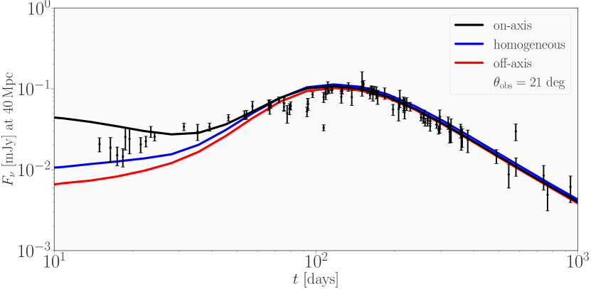
Figure 9: Comparison of the radio afterglow from GW170817 (black circles with corresponding error bars) with the afterglow light-curves relative to model Lj.5.49.Me.004 for an observer with viewing angle $\theta_{\rm obs}=21\,{\rm deg}$. The different lines refer to the different anisotropies in the ejecta (red line for off-axis, blue line for on-axis and black line for the homogeneous distribution). The data is taken at a frequency of $\nu=6\,\mathrm{GHz}$ and up until $940\,\mathrm{d}$ after the burst.

3.5 On the use of afterglows to study jet structures

The afterglows of relativistic outflows can obviously be used to infer the structure of these jets. This structure can, in turn, provide insight on the physics at smaller scales, on the launching of the jet by the central engine and its interaction with the merger ejecta. Overall, our simulations show that the interaction of the jet with the ejecta, quite independently of their geometric anisotropic properties, leads to an energy polar structure of the jet that is characterised by a steep segment followed by a shallow segment can arise from jet-ejecta interaction (cf., Fig. 7), and that the extent of the shallow segment depends on the strength of this interaction as measured by the ratio of the ejecta mass and of the jet luminosity, $M_{\rm ej}/L_{\rm jet}$ ratio. Interestingly, to our knowledge, this double steep-shallow-segment jet structure in energy has not been found in previous study of jet-ejecta interaction, and has not been considered as a functional form for the fitting of afterglow data. It does, however, appear as a possible jet structure reconstructed directly from the afterglow data of GRB170817A (Takahashi & Ioka, 2021). In particular, as shown in Fig. 8, this structure can give rise to a variety of afterglow morphologies for off-axis observers, from a fast-rise-fast-decline for very small interactions resulting in near top-hat structures (e.g., Lj.1.50.Me.001) to slow-rise-fast-decline for moderate interaction resulting in a reduced shallow segment (e.g., Lj.1.50.Me.010) and a double-peaked afterglow for significant interaction resulting in a large energy reservoir at high-latitudes (e.g., Lj.5.49.Me.010). Analytical studies have shown that this variety of light-curve morphologies can also arise from simple power-law structures (Beniamini et al., 2020b), underlining once more the large degeneracy (and risks) in reconstructing structure from afterglow light-curves. As an additional caveat, our simulations also highlight that differences in the distribution of the rest-mass density of the ejecta can have a strong impact on the large-scale structure of the jet and of the cocoon. This makes the inferring of the ejecta properties more challenging even when assuming a perfect knowledge of the jet structure. At the same time, the simulations also show that the impact of the ejecta properties depends systematically on both the jet luminosity $L_{\rm jet}$ to the ejecta mass $M_{\rm ej}$, and has a regular behaviour with their ratio.

We should also remark that the effect of the jet energy structure has also been recently considered on slightly misaligned lines of sight, i.e., with $\theta_{\rm obs}\lesssim 2\times\theta_{\rm jet}$, in relation to the origin of plateaus (Eichler & Granot, 2006; Beniamini et al., 2020a) or of flares in SGRB afterglows (Duque et al., 2022). The models explored in these studies generally require a steep jet structure in this near-core range of angles, in apparent tension with the shallow structure on large angles revealed in the jet of GRB170817A when fit with single power-law structures (Ghirlanda et al., 2019; Gill & Granot, 2018). However, the double steep-shallow structure revealed by our simulations naturally reconciles these two observational properties, with the steep segment allowing for these plateaus and flare models on slightly misaligned lines of sight and for a GRB170817A-like afterglows on significantly misaligned ones.

Finally, we note that in the case of GRB170817, the ejecta mass inferred from the kilonova observations is $\gtrsim 0.01M_{\rm\odot}$ (Villar et al., 2017; Metzger et al., 2018; Coughlin et al., 2019) and the iso-equivalent energy of the core jet inferred from the afterglow photometry and image is of $\sim 10^{52}\,{\rm erg}$, within a core angle of $\theta_{\rm jet}\sim 6\,\rm{deg}$ (Ghirlanda et al., 2019). Assuming a jet duration of $\Delta t=1\,{\rm s}$ and negligible losses to SGRB prompt emission and jet-ejecta interactions in the core jet, this would translate into a jet luminosity of $L_{\rm jet}\sim 5\times 10^{49}\,{\rm erg/s}$. This places GRB170817 in the regime of our Lj.5.49.Me.010 simulation, where we expect significant interaction of the jet with the ejecta and a strong effect on the high-latitude energy structure of the jet. On the one hand, this would be compatible with the GRB170817 afterglow and its extended slowly-increasing phase (Mooley et al., 2018c) as due, in our simulations, to a strong jet-ejecta interaction after launch. On the other hand, this conclusion would cast doubts about the possibility of using the afterglow in infer ejecta properties, since in this regime we have shown the sensitivity to ejecta details.

In summary, our simulations show that a great diversity of afterglow light-curve morphologies can arise due to the jet-ejecta interactions. This suggests that the afterglow of GW170817 could not be a standard for BNS merger afterglows, as future GW follow-up observations could reveal. As a result, our systematic investigation reveals that the role of the ejecta in shaping this afterglow provides an additional caveat on inference of the jet structure from the afterglow observations, which fortunately is less important for lower $M_{\rm ej}/L_{\rm jet}$ ratios. Indeed, if this ratio could be determined to be small using a independent method (e.g., based on the kilonova signal), then reconstructing the jet from the afterglow data will likely be more robust and carry less uncertainty.

4 Conclusions

Using general-relativistic hydrodynamical simulations, we have examined the propagation of an ultra-relativistic jet through an envelope of matter ejected by a BNS merger having a variety of anisotropic distributions of rest-mass. Overall, our results can be summarised as follows.

• The geometry and degree of anisotropy of the ejecta impacts the propagation of the jet and influences its breakout time as well as the energy in the cocoon produced.

• Contrary to expectations, the propagation of a jet encountering several anisotropies along its path (i.e., on-axis perturbations) only marginally affects its breakout time, which is comparable with that in the absence of anisotropies.

• The breakout time decreases as the energy of the jet is increased and increases as the ejected matter is more massive. This is simply because the jet travel-time across the ejecta will depend on its energy and on the matter resistance it will encounter. As a result, the most massive ejecta actually prevent the breakout of the weakest jet.

• The time-averaged efficiency $\langle\epsilon\rangle$ in the conversion of the jet kinetic energy into the thermal energy of the cocoon decreases linearly with increasing energy in the jet and with the mass in the ejecta. This behaviour reflects the fact that more energetic jets are less efficient in converting the kinetic energy into thermal energy, especially if the ejecta are not very massive.

• In agreement with Duffell et al. (2018), $\langle\epsilon\rangle$, but also the average thermal energy $\langle E_{\rm th}\rangle$ and the peak internal energy $E_{\rm th,peak}$, show a square-root scaling with the jet energy and a linear scaling with the mass in the ejecta. The variance produced by the different types of anisotropies is marginal and most important at the largest jet luminosities.

• The injection of internal energy into the matter in the cocoon by the propagating jet is sufficiently large to allow for the escape of this energy from the ejecta. The amount of energy in the cocoon that is able to escape $E_{\rm coc}$ grows with both the energy in the jet and with the mass in the ejecta.

• Given an ejecta mass and a jet propagating at a given luminosity, a critical efficiency of $\eta_{\rm crit}\sim{L_{\rm jet,50}\,(t_{\rm jet,bo}/1\,{\rm s})}(M_{\rm ej}/{10^{-3}\,M_{\odot}})^{-1}\sim 0.03$ exists for a successful jet breakout after a time $t_{\rm jet,bo}$.

• Essentially all configurations considered show a similar two-component behaviour for the polar structure of the jet. In particular, the polar profiles of the Lorentz factor consistently show a “core” with $\Gamma_{\infty}\sim 60-90$ within an angle of $\theta\approx 5\,\mathrm{deg}$. The Lorentz factor then exhibits a sharp decrease down to $\Gamma_{\infty}\lesssim 10$ for $\theta\gtrsim 7\,{\rm deg}$ with a power-law dependence $\Gamma_{\infty}(\theta)\propto\theta^{-\beta}$ with $\beta>7$. The polar structure of the energy distribution, on the other hand, does not have a sharp fall-off but a much slower decay ranging from a flat distribution to power-law decays with index $\beta\sim 3$ up to large latitudes up to $\theta\approx 25\,\mathrm{deg}$.

• Within the two-components structure of the jet, the core is essentially unaffected by the anisotropies in the ejecta, while the shallow segment displays the greatest variance, which is stronger for lower ratios of $L_{\mathrm{jet}}/M_{\mathrm{ej}}$. In the case of the marginally successful jet, on the other hand, the two-components structure is essentially not present and the polar distributions of energy and Lorentz factor are far more irregular.

• Different anisotropies impact the variance of the afterglow light-curves as a function of the jet luminosity and ejected mass. In particular, the variance is reduced as the injected energy in the jet is increased $L_{\rm jet}$, but it increases with the mass in the ejecta $M_{\rm ej}$. As a result, the impact of the anisotropies in the ejecta effectively increases with the ratio $M_{\rm ej}/L_{\rm jet}$.

• The anisotropies in the afterglow observations are most dominant in the first tens of days, for off-axis observations of systems with generally high ejecta mass. In the case of BNS mergers, strong candidates for detection of these effects, are the systems with low mass ratio $q:=M_{2}/M_{1}$, where $M_{1}$ is the mass of the primary and $M_{2}$ that of the secondary. The reason for this is that these systems generally produce larger amounts of dynamically ejected matter.

• Double-peaks in the light-curves can also arise from the polar structure of the energy distribution of the jet, provided it has two portions, with a steep inner core and a shallow exterior with a local maximum at large latitudes. This represents a further illustration of the degeneracies that can be present when in inferring jet structures from afterglow light-curves.

• The presence of an extended shallow segment in the jet structure for systems with moderate $L_{\rm jet}/M_{\rm ej}$ ratios results in long-lasting phases of slow brightening of the afterglow as the emission is dominated by material progressively ranging up the shallow segment (cf., GRB170817A).

• In the case of GRB170817A, assuming a jet duration of $\Delta t=1\,{\rm s}$ and negligible losses to GRB prompt emission and jet-ejecta interactions in the core jet, leads to a jet luminosity of $L_{\rm jet}\sim 5\times 10^{49}\,{\rm erg/s}$. This is in the regime where we expect significant interaction of the jet with the ejecta and a strong effect on the high-latitude energy structure of the jet.

While the present work arguably represents the most extended and systematic investigation of the interaction of a relativistic jet with the ejecta from a BNS merger with non-smooth features in the density distribution, it can be improved in at least three different directions. First, by including the presence of a magnetic field of different topologies and strengths (Nathanail et al., 2020, 2021), which could influence the propagation of the jet across the ejecta and that, in the presence of turbulence-driven reconnection, could lead to an increase of the internal energy of the cocoon. Second, by extending to three the number of spatial dimensions, which would improve the description of the dynamics of the jet head and remove some of the artefacts discussed here. Finally, by moving away from the simple equation of state considered in our work and by considering instead the same equations of state describing the neutron-star matter in full numerical-relativity calculations. This final step, which is less trivial than it may appear given the complexity of the equations of state employed in BNS mergers, will finally allow for a consistent and faithful import of realistic ejecta distributions from merger simulations.

As a concluding remark, we note how future gravitational-wave observing runs will see more afterglows of jets with significantly off-axis lines of sight, both with current facilities (e.g., Duque et al., 2019; Colombo et al., 2022) and with next-generation instruments (Ronchini et al., 2022), thus allowing for deeper insights into the jet structure. In view of our results, the combination of this data with kilonovae signals (see, e.g.,  Mochkovitch et al., 2021) could provide a very powerful tool to understand the properties of the sources. Indeed, if dim kilonova signals were to be more often associated with rapidly-increasing afterglows, they could provide the signature of a small ejecta mass weakly imprinting the incipient jet, which therefore retained its steep initial structure as described here. In this case, the incipient jet structures could be considered a faithful probe of the jet-launching physics at the scales of the central engine. If, on the contrary, dim kilonovae were to be most regularly associated with slowly-increasing afterglows, they could hint to the fact that the associated shallow jet structures are acquired directly at jet launch. Finally, the inclusion of gravitational-wave constraints on the progenitor binaries can help bridge the gap between the kilonova and afterglow jet signals with the theoretical predictions obtained by numerical simulations on the ability of magnetised merging BNSs to launch relativistic jets (see, e.g.,  Rezzolla et al., 2011; Hotokezaka et al., 2013; Palenzuela et al., 2015; Ruiz et al., 2016).

Data Availability

The data underlying this article will be shared on reasonable request to the corresponding author.

Appendix A Numerical consistency and robustness of the results

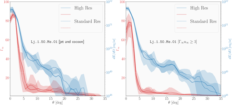
Figure 10: The same as in Fig. 7 for model Lj.1.50.Me.010 at $t=2.25\,\mathrm{s}$ after jet launching. The solid and dashed lines refer to simulations performed with a numerical resolution that is either “high” or “standard”, respectively. Clearly, the qualitative features of the polar structures are robust and no new features are introduced when increasing the resolution.

In this Appendix, we study the consistency and the robustness of our results to the choice of resolution for our numerical simulations. We focus on the main result extracted from our simulation domain: the energy and Lorentz-factor structures of the relativistic jets after breakout from the ejecta.

We proceed with the method described in Sec. 2.2 considering two different numerical resolutions: the first, referred to as “standard resolution”, is as provided in Sec. 2.1 with a mesh of $N_{r}\times N_{\theta}=1120\times 576$ cells and three refinement levels; the second resolution, dubbed “high resolution”, is 1.5 times finer with a base grid of $N_{r}\times N_{\theta}=1680\times 864$ and three adaptive refinement levels.

In Fig. 10, we report the results for the Lj.1.50.Me.010 system using the two resolution levels, presenting the energy ${\rm d}E_{\rm jet}/{\rm d}\Omega(\theta)$ and Lorentz-factor, $\Gamma_{\infty}(\theta)$ structures in analogy with Fig. 7 of the main text. As in the main text, we report the structured obtained by applying two different cuts in the Lorentz-factor, aiming to capture the jet and cocoon material, or only the high-velocity jet. We find that, within the variance induced by the three choices of the density profiles of the eject, the results are consistent for the two resolutions. This is the case for both the choices of velocity cuts, with the highest fidelity between the two resolutions found for the high-velocity structures.

In particular, the presence of a large energy reservoir at high-latitudes is a robust feature, and the energy level and angular extent of this reservoir is consistent between the runs with different resolution. The run presented in Fig. 10 has the largest ejecta mass among our runs, such that the effect on the jet is expected to be among the largest. Since this behaviour is properly captured and exhibits consistency between the two resolutions, we conclude that the results of the other runs are also robust and can be used to derive reliably the conclusions drawn in the main text.

References

- Abbott et al. (2017) Abbott B. P., et al., 2017, ApJ, 848, L12
- Alexander et al. (2017) Alexander K. D., et al., 2017, ApJ, 848, L21
- Aloy et al. (2005) Aloy M. A., Janka H. T., Müller E., 2005, A&A, 436, 273
- Arcavi et al. (2017) Arcavi I., et al., 2017, Nature, 551, 64
- Baiotti & Rezzolla (2017) Baiotti L., Rezzolla L., 2017, Rept. Prog. Phys., 80, 096901
- Bauswein et al. (2013) Bauswein A., Goriely S., Janka H. T., 2013, ApJ, 773, 78
- Beniamini et al. (2020a) Beniamini P., Granot J., Gill R., 2020a, MNRAS, 493, 3521
- Beniamini et al. (2020b) Beniamini P., Duran R. B., Petropoulou M., Giannios D., 2020b, ApJ, 895, L33
- Blandford & McKee (1976) Blandford R. D., McKee C. F., 1976, Physics of Fluids, 19, 1130
- Bovard et al. (2017) Bovard L., Martin D., Guercilena F., Arcones A., Rezzolla L., Korobkin O., 2017, Phys. Rev. D, 96, 124005
- Bromberg et al. (2011) Bromberg O., Nakar E., Piran T., Sari R., 2011, ApJ, 740, 100
- Cenko et al. (2011) Cenko S. B., et al., 2011, ApJ, 732, 29
- Colombo et al. (2022) Colombo A., Salafia O. S., Gabrielli F., Ghirlanda G., Giacomazzo B., Perego A., Colpi M., 2022, ApJ, 937, 79
- Combi & Siegel (2023) Combi L., Siegel D. M., 2023, ApJ, 944, 28
- Coughlin et al. (2019) Coughlin M. W., Dietrich T., Margalit B., Metzger B. D., 2019, Monthly Notices of the Royal Astronomical Society: Letters, 489, L91
- Crumley et al. (2019) Crumley P., Caprioli D., Markoff S., Spitkovsky A., 2019, MNRAS, 485, 5105
- D’Avanzo et al. (2018) D’Avanzo P., et al., 2018, A&A, 613, L1
- Dessart et al. (2009) Dessart L., Ott C. D., Burrows A., Rosswog S., Livne E., 2009, ApJ, 690, 1681
- Dietrich et al. (2017) Dietrich T., Bernuzzi S., Ujevic M., Tichy W., 2017, Phys. Rev. D, 95, 044045
- Dionysopoulou et al. (2015) Dionysopoulou K., Alic D., Rezzolla L., 2015, Phys. Rev. D, 92, 084064
- Dobie et al. (2018) Dobie D., et al., 2018, ApJ, 858, L15
- Drout et al. (2017) Drout M. R., et al., 2017, Science, 358, 1570
- Duffell et al. (2018) Duffell P. C., Quataert E., Kasen D., Klion H., 2018, Astrophys. J., 866, 3
- Duque et al. (2019) Duque R., Daigne F., Mochkovitch R., 2019, A&A, 631, A39
- Duque et al. (2020) Duque R., Beniamini P., Daigne F., Mochkovitch R., 2020, A&A, 639, A15
- Duque et al. (2022) Duque R., Beniamini P., Daigne F., Mochkovitch R., 2022, MNRAS, 513, 951
- Eichler & Granot (2006) Eichler D., Granot J., 2006, ApJ, 641, L5
- Eichler et al. (1989) Eichler D., Livio M., Piran T., Schramm D. N., 1989, Nature, 340, 126
- Evans et al. (2017) Evans P. A., et al., 2017, Science, 358, 1565
- Fernández et al. (2015) Fernández R., Kasen D., Metzger B. D., Quataert E., 2015, MNRAS, 446, 750
- Fong et al. (2019) Fong W., et al., 2019, ApJ, 883, L1
- Foucart et al. (2016) Foucart F., O’Connor E., Roberts L., Kidder L. E., Pfeiffer H. P., Scheel M. A., 2016, Phys. Rev. D, 94, 123016
- Fujibayashi et al. (2018) Fujibayashi S., Kiuchi K., Nishimura N., Sekiguchi Y., Shibata M., 2018, ApJ, 860, 64
- Fujibayashi et al. (2023) Fujibayashi S., Kiuchi K., Wanajo S., Kyutoku K., Sekiguchi Y., Shibata M., 2023, ApJ, 942, 39
- Ghirlanda et al. (2019) Ghirlanda G., et al., 2019, Science, 363, 968
- Gill & Granot (2018) Gill R., Granot J., 2018, Mon. Not. R. Astron. Soc.,
- Gill et al. (2019) Gill R., Nathanail A., Rezzolla L., 2019, ApJ, 876, 139
- Goldstein et al. (2017) Goldstein A., et al., 2017, Astrophys. J. Letters, 848, L14
- Gottlieb & Globus (2021) Gottlieb O., Globus N., 2021, ApJ, 915, L4
- Gottlieb & Nakar (2022) Gottlieb O., Nakar E., 2022, MNRAS, 517, 1640
- Gottlieb et al. (2018) Gottlieb O., Nakar E., Piran T., Hotokezaka K., 2018, MNRAS, 479, 588
- Gottlieb et al. (2019) Gottlieb O., Levinson A., Nakar E., 2019, MNRAS, 488, 1416
- Gottlieb et al. (2020a) Gottlieb O., Bromberg O., Singh C. B., Nakar E., 2020a, MNRAS, 498, 3320
- Gottlieb et al. (2020b) Gottlieb O., Nakar E., Bromberg O., 2020b, Monthly Notices of the Royal Astronomical Society, 500, 3511
- Gottlieb et al. (2022) Gottlieb O., Moseley S., Ramirez-Aguilar T., Murguia-Berthier A., Liska M., Tchekhovskoy A., 2022, ApJ, 933, L2
- Granot & Sari (2002) Granot J., Sari R., 2002, ApJ, 568, 820
- Granot et al. (1999) Granot J., Piran T., Sari R., 1999, The Astrophysical Journal, 527, 236
- Granot et al. (2002) Granot J., Panaitescu A., Kumar P., Woosley S. E., 2002, ApJ, 570, L61
- Hajela et al. (2019) Hajela A., et al., 2019, ApJ, 886, L17
- Hallinan et al. (2017) Hallinan G., et al., 2017, Science, 358, 1579
- Hamidani & Ioka (2023) Hamidani H., Ioka K., 2023, MNRAS, 520, 1111
- Hayashi et al. (2022) Hayashi K., Fujibayashi S., Kiuchi K., Kyutoku K., Sekiguchi Y., Shibata M., 2022, Phys. Rev. D, 106, 023008
- Hotokezaka et al. (2013) Hotokezaka K., Kiuchi K., Kyutoku K., Okawa H., Sekiguchi Y.-i., Shibata M., Taniguchi K., 2013, Phys. Rev. D, 87, 024001
- Kasen et al. (2017) Kasen D., Metzger B., Barnes J., Quataert E., Ramirez-Ruiz E., 2017, Nature, 551, 80
- Kasliwal et al. (2017) Kasliwal M. M., et al., 2017, Science, 358, 1559
- Kilpatrick et al. (2017) Kilpatrick C. D., et al., 2017, Science, 358, 1583
- LIGO Scientific Collaboration et al. (2017) LIGO Scientific Collaboration et al., 2017, Astrophys. J. Lett., 848, L13
- Lamb et al. (2018) Lamb G. P., Mandel I., Resmi L., 2018, MNRAS, 481, 2581
- Lamb et al. (2019) Lamb G. P., et al., 2019, ApJ, 870, L15
- Lamb et al. (2021) Lamb G. P., Kann D. A., Fernández J. J., Mandel I., Levan A. J., Tanvir N. R., 2021, MNRAS, 506, 4163
- Lazzati et al. (2018) Lazzati D., Perna R., Morsony B. J., Lopez-Camara D., Cantiello M., Ciolfi R., Giacomazzo B., Workman J. C., 2018, Phys. Rev. Lett., 120, 241103
- Lazzati et al. (2021) Lazzati D., Perna R., Ciolfi R., Giacomazzo B., López-Cámara D., Morsony B., 2021, ApJ, 918, L6
- Lehner et al. (2016) Lehner L., Liebling S. L., Palenzuela C., Caballero O. L., O’Connor E., Anderson M., Neilsen D., 2016, Classical and Quantum Gravity, 33, 184002
- López-Cámara et al. (2013) López-Cámara D., Morsony B. J., Begelman M. C., Lazzati D., 2013, ApJ, 767, 19
- Lyman et al. (2018) Lyman J. D., et al., 2018, Nature Astronomy, 2, 751
- Makhathini et al. (2021) Makhathini S., et al., 2021, ApJ, 922, 154
- Margutti et al. (2017) Margutti R., et al., 2017, ApJ, 848, L20
- Matsumoto et al. (2019) Matsumoto T., Nakar E., Piran T., 2019, MNRAS, 483, 1247
- Meringolo et al. (2023) Meringolo C., Cruz-Osorio A., Rezzolla L., Servidio S., 2023, Astrophys. J., 944, 122
- Metzger et al. (2018) Metzger B. D., Thompson T. A., Quataert E., 2018, ApJ, 856, 101
- Mizuta & Ioka (2013) Mizuta A., Ioka K., 2013, The Astrophysical Journal, 777, 162
- Mochkovitch et al. (2021) Mochkovitch R., Daigne F., Duque R., Zitouni H., 2021, A&A, 651, A83
- Mooley et al. (2018a) Mooley K. P., et al., 2018a, Nature, 554, 207
- Mooley et al. (2018b) Mooley K. P., et al., 2018b, Nature, 561, 355
- Mooley et al. (2018c) Mooley K. P., et al., 2018c, ApJ, 868, L11
- Morlino & Caprioli (2012) Morlino G., Caprioli D., 2012, A&A, 538, A81
- Most et al. (2019) Most E. R., Papenfort L. J., Tsokaros A., Rezzolla L., 2019, ApJ, 884, 40
- Most et al. (2021) Most E. R., Papenfort L. J., Tootle S. D., Rezzolla L., 2021, MNRAS, 506, 3511
- Murguia-Berthier et al. (2016) Murguia-Berthier A., et al., 2016, Astrophys. J. Lett., 835, L34
- Murguia-Berthier et al. (2021) Murguia-Berthier A., Ramirez-Ruiz E., De Colle F., Janiuk A., Rosswog S., Lee W. H., 2021, ApJ, 908, 152
- Nagakura et al. (2014) Nagakura H., Hotokezaka K., Sekiguchi Y., Shibata M., Ioka K., 2014, ApJ, 784, L28
- Nakar & Piran (2017) Nakar E., Piran T., 2017, ApJ, 834, 28
- Nakar et al. (2002) Nakar E., Piran T., Granot J., 2002, ApJ, 579, 699
- Nathanail et al. (2019) Nathanail A., Porth O., Rezzolla L., 2019, ApJ, 870, L20
- Nathanail et al. (2020) Nathanail A., Gill R., Porth O., Fromm C. M., Rezzolla L., 2020, Mon. Not. R. Astron. Soc., 495, 3780
- Nathanail et al. (2021) Nathanail A., Gill R., Porth O., Fromm C. M., Rezzolla L., 2021, MNRAS, 502, 1843
- Nynka et al. (2018) Nynka M., Ruan J. J., Haggard D., Evans P. A., 2018, ApJ, 862, L19
- Olivares et al. (2019) Olivares H., Porth O., Davelaar J., Most E. R., Fromm C. M., Mizuno Y., Younsi Z., Rezzolla L., 2019, Astron. Astrophys., 629, A61
- Paczynski (1986) Paczynski B., 1986, ApJ, 308, L43
- Palenzuela et al. (2015) Palenzuela C., Liebling S. L., Neilsen D., Lehner L., Caballero O. L., O’Connor E., Anderson M., 2015, Phys. Rev. D, 92, 044045
- Panaitescu & Kumar (2000) Panaitescu A., Kumar P., 2000, The Astrophysical Journal, 543, 66
- Paschalidis (2017) Paschalidis V., 2017, Classical and Quantum Gravity, 34, 084002
- Pavan et al. (2021) Pavan A., Ciolfi R., Kalinani J. V., Mignone A., 2021, MNRAS, 506, 3483
- Pian et al. (2017) Pian E., et al., 2017, Nature, 551, 67
- Piro & Kollmeier (2018) Piro A. L., Kollmeier J. A., 2018, ApJ, 855, 103
- Porth et al. (2017) Porth O., Olivares H., Mizuno Y., Younsi Z., Rezzolla L., Moscibrodzka M., Falcke H., Kramer M., 2017, Computational Astrophysics and Cosmology, 4, 1
- Radice et al. (2016) Radice D., Galeazzi F., Lippuner J., Roberts L. F., Ott C. D., Rezzolla L., 2016, Monthly Notices of the Royal Astronomical Society, 460, 3255
- Radice et al. (2018) Radice D., Perego A., Hotokezaka K., Fromm S. A., Bernuzzi S., Roberts L. F., 2018, The Astrophysical Journal, 869, 130
- Rezzolla & Zanotti (2013) Rezzolla L., Zanotti O., 2013, Relativistic Hydrodynamics. Oxford University Press, Oxford, UK, doi:10.1093/acprof:oso/9780198528906.001.0001
- Rezzolla et al. (2010) Rezzolla L., Baiotti L., Giacomazzo B., Link D., Font J. A., 2010, Classical and Quantum Gravity, 27, 114105
- Rezzolla et al. (2011) Rezzolla L., Giacomazzo B., Baiotti L., Granot J., Kouveliotou C., Aloy M. A., 2011, Astrophys. J. Letters, 732, L6
- Ronchini et al. (2022) Ronchini S., et al., 2022, A&A, 665, A97
- Ruiz et al. (2016) Ruiz M., Lang R. N., Paschalidis V., Shapiro S. L., 2016, Astrophys. J. Lett., 824, L6
- Ruiz et al. (2020) Ruiz M., Paschalidis V., Tsokaros A., Shapiro S. L., 2020, Phys. Rev. D, 102, 124077
- Salafia & Ghirlanda (2022) Salafia O. S., Ghirlanda G., 2022, Galaxies, 10
- Salafia et al. (2019) Salafia O. S., Ghirlanda G., Ascenzi S., Ghisellini G., 2019, A&A, 628, A18
- Sari et al. (1998) Sari R., Piran T., Narayan R., 1998, ApJ, 497, L17
- Sekiguchi et al. (2015) Sekiguchi Y., Kiuchi K., Kyutoku K., Shibata M., 2015, Phys. Rev. D, 91, 064059
- Shappee et al. (2017) Shappee B. J., et al., 2017, Science, 358, 1574
- Shibata & Hotokezaka (2019) Shibata M., Hotokezaka K., 2019, Annual Review of Nuclear and Particle Science, 69, 41
- Siegel et al. (2014) Siegel D. M., Ciolfi R., Rezzolla L., 2014, Astrophys. J., 785, L6
- Sironi & Spitkovsky (2011) Sironi L., Spitkovsky A., 2011, ApJ, 726, 75
- Sironi et al. (2013) Sironi L., Spitkovsky A., Arons J., 2013, ApJ, 771, 54
- Smartt et al. (2017) Smartt S. J., et al., 2017, Nature, 551, 75
- Takahashi & Ioka (2020) Takahashi K., Ioka K., 2020, MNRAS, 497, 1217
- Takahashi & Ioka (2021) Takahashi K., Ioka K., 2021, MNRAS, 501, 5746
- The LIGO Scientific Collaboration & The Virgo Collaboration (2017) The LIGO Scientific Collaboration The Virgo Collaboration 2017, Phys. Rev. Lett., 119, 161101
- The LIGO Scientific Collaboration et al. (2017) The LIGO Scientific Collaboration et al., 2017, Astrophys. J. Lett., 848, L12
- Troja et al. (2017) Troja E., et al., 2017, Nature, 551, 71
- Troja et al. (2018) Troja E., et al., 2018, MNRAS, 478, L18
- Troja et al. (2019) Troja E., et al., 2019, MNRAS, 489, 1919
- Urrutia et al. (2021) Urrutia G., De Colle F., Murguia-Berthier A., Ramirez-Ruiz E., 2021, MNRAS, 503, 4363
- Villar et al. (2017) Villar V. A., et al., 2017, ApJ, 851, L21
- Wang et al. (2023) Wang Y.-Y., Tang S.-P., Jin Z.-P., Fan Y.-Z., 2023, ApJ, 943, 13
- Watson et al. (2019) Watson D., et al., 2019, Nature, 574, 497
- Zhang et al. (2004) Zhang W., Woosley S. E., Heger A., 2004, The Astrophysical Journal, 608, 365