A perturbation theory for the Coulomb phase infrared-divergence

Abstract

We construct a perturbation theory which we conjecture to be free of the Coulomb-phase infrared divergence. This perturbation theory is developed for one of the simplest yet prototypical scattering amplitudes which would otherwise exhibit this divergence: the semiclassical scattering of a spinless boson on a background Coulomb field. The perturbation theory is based upon replacing plane waves with Coulomb wavefunctions, and the free-field propagator with the Coulomb propagator, in order to appropriately match the asymptotics of the exact in/out states. We compute the leading-order (LO) and next-to-leading-order (NLO) infrared-finite scattering amplitudes in this framework, which include all-order-in-the-coupling effects, and demonstrate that these amplitudes are in agreement with the known exact amplitude at these orders. We comment on the Runge-Lenz symmetry of the LO amplitude which occurs as a principal series representation of the Euclidean conformal group on the $2$-sphere.

1 Introduction

Infrared divergences occur in interacting theories that contain massless particles in four or fewer spacetime dimensions, and are thus of considerable importance for the Standard Model of particle physics. These divergences can be alleviated on the level of inclusive cross-sections for sufficiently simple theories like QED Bloch:1937pw . However, in order to study questions regarding causality and unitarity it is preferable to alleviate these divergences on the level of amplitudes, ideally without introducing an IR-cutoff. The Faddeev-Kulish (FK) framework Kulish:1970ut ; Dollard1964AsymptoticCA ; Kibble:1968sfb ; Chung:1965zza represents one solution to the problem of constructing an IR-finite S-matrix, and while it has been useful for uncovering many features of the infrared structure of gauge theories and gravity, it has rarely been used for the explicit calculation of IR-finite scattering amplitudes, with Hannesdottir:2019opa ; Hannesdottir:2019umk ; Forde:2003jt being the only instances of explicitly calculated amplitudes we were able to find.

One of the simplest examples of an infrared divergence is encountered when using standard techniques to compute the semiclassical scattering of a Klein-Gordon (KG) particle off a Coulomb background kang1962higher . In this paper, we construct a perturbation theory, conjectured to be IR-finite, for this semiclassical amplitude and calculate it up to the NLO. The LO (65) and NLO (83) amplitudes are IR-finite and do not contain any implicit or explicit cut-off or dimensional regularization scale. The exact IR-finite amplitude (87) is known by other non-perturbative means, and we find agreement with this result up to the orders we compute, thus providing confidence for extending the perturbation theory to less trivial settings where the exact answer is not known.

The underlying cause of infrared divergences, both in the semiclassical and the quantum cases, is that states in such theories do not appropriately converge towards non-interacting free particle states at asymptotic times, which is counter to an assumption of standard perturbation theory. This does not imply that scattering amplitudes are ambiguous, zero, infinite, or cut-off dependent, it only implies that one should not use a perturbation theory that assumes asymptotically non-interacting states. In the semiclassical case, it is this assumption regarding asymptotically non-interacting particles which leads to the use of plane-waves as a useful basis of wavefunctions for perturbatively constructing the amplitude. In the presence of long-range forces it would be preferable to use a basis of wavefunctions whose asymptotics appropriately match those of the exact in/out states. In this paper we develop a perturbation theory which uses a basis of wavefunctions, Coulomb wavefunctions, whose asymptotic behaviour appropriately matches those of the exact in/out states, namely the perturbation theory implements the replacement

$$e^{-ip\cdot x}\rightarrow e^{-ip\cdot x}{}_{1}F_{1}\Big{(}-i\frac{e_{1}e_{2}}{4\pi}\frac{E}{|\vec{p}|},1,i(|\vec{p}||\vec{x}|-\vec{p}\cdot\vec{x})\Big{)}$$ (1)

(the Lorentz invariant form of the RHS is given at (39, 40)) where ${}_{1}F_{1}(a,b,z)$ is the confluent hypergeometric function, $e_{1}e_{2}$ are the charges of the particles, and when we turn off the coupling we recover standard plane waves ${}_{1}F_{1}(0,a,b)=1$. Let us be quick to emphasize that when implementing the replacement (1) we will not be redefining the scattering amplitude, nor will we be scattering wave-packets. The infrared-finite semiclassical scattering amplitude is unambiguously defined, as we review in section 3, without any reference to the perturbation theory one uses to compute it. Whether one uses plane-waves or Coulomb wavefunctions is a matter of framework. If one uses plane-waves, then in order to account for the disagreement between the asymptotics, one has to implement the Faddeev-Kulish approach by modifying the evolution operators. Instead if we use Coulomb wavefunctions, then the asymptotics agree, and the modification to the evolution operators is much simpler. Both approaches should give the same answer, as they are both computing a quantity that is independent of the perturbative framework. To demonstrate this equivalence, in section 4.3 we argue that the relevant Faddeev-Kulish Moller operators act as a projection operators which implement the mapping (1).

Infrared divergences make the causality and unitarity properties of observables in QFT less transparent. For example, many of the most useful theorems concerning the analytic structure of S-matrices in $4D$, such as the Froissart-Martin bound and the Steinmann relations Steinmann1960 , require the existence of a mass-gap, which is somewhat disappointing seeing that QED and gravity do not have a mass gap. Without firm control over the cut-off independent IR-finite S-matrix, it is significantly more difficult to study the analytic structure of observables in gapless $4D$ QFTs, and deduce the analogs of these theorems Bourjaily:2020wvq ; Fevola:2023fzn ; Berghoff:2022mqu ; Hannesdottir:2022xki . Properties such as these are of central importance in the modern day S-matrix bootstrap program deRham:2022hpx ; Kruczenski:2022lot , as well as for a variety of modern day techniques for calculating observables in QFT caronhuot2020steinmann , thus it would be beneficial to have a framework which gives IR-finite, cut-off independent, unambiguous, scattering amplitudes.

There are three distinct phenomena which are generally referred to as infrared-divergences: collinear, real emission, and imaginary (or Coulomb phase) divergences, and this article only addresses the last one of these. Collinear divergences arise in theories which contain vertices where three massless particles can meet. We will not study such theories in this paper. The distinction between real and imaginary infrared divergences can be explained by looking at the soft exponentiation factor for the leading infrared divergences in abelian gauge theories yennie ; Weinberg:1965nx . This theorem states that the leading IR-divergences in an abelian gauge theory can be factored out of the scattering amplitude $\mathcal{A}$ (see Eq.13.2.4 of Weinberg:1995mt for a textbook discussion)

$$\mathcal{A}=\Bigg{(}\frac{\Lambda_{\text{IR}}}{\lambda_{\text{IR}}}\Bigg{)}^{R+I}\mathcal{A}_{0}(\Lambda_{\text{IR}}),$$ (2)

where the real and imaginary parts are respectively

$$R=\frac{1}{16\pi^{2}}\sum_{i,j}\frac{\eta_{i}\eta_{j}e_{i}e_{j}}{\beta_{ij}}\log\Big{(}\frac{1+\beta_{ij}}{1-\beta_{ij}}\Big{)}\quad,\quad I=\frac{1}{8\pi}\sum_{\eta_{i}\eta_{j}=+}-i\frac{e_{i}e_{j}}{\beta_{ij}},$$ (3)

$$\beta_{ij}\coloneqq\sqrt{1-\frac{m_{i}^{2}m_{j}^{2}}{(p_{i}\cdot p_{j})^{2}}},$$ (4)

where $\eta=+/-$ corresponds to in/out states, respectively, $\lambda_{\text{IR}}/\Lambda_{\text{IR}}$ represent the lower/upper infrared (IR) cutoff scales for the energies of exchanged photons, and $\mathcal{A}_{0}(\Lambda_{\text{IR}})$ only contains photon exchanges with energies greater than $\Lambda_{\text{IR}}$. The real factor $R$ in (3) is related to the production of real photons, as it is this term which cancels out on the level of inclusive cross-sections when summing over soft radiatiative processes. We will not consider this term any further, and explain in Sect. 3 how by using a retarded propagator for the gauge fields we are able to avoid dealing with this term, so that we can isolate the focus of this work, the Coulomb phase divergence. The second term in (3) is referred to as the Coulomb phase divergence and it is purely imaginary. The $\eta_{i}\eta_{j}=+1$ indicates that this term only occurs for pairs of particles that are both in or both out states. Physically, one can associate the Coulomb phase divergence to the fact that the late time trajectories of classical particles interacting via a $\frac{1}{r}$-potential do not asymptote to free particle trajectories, but hyperbolic trajectories which have a logarithmic correction to free particle motion (see e.g. PhysRevD.7.1082 ; Sahoo_2019 for the trajectory, and appendix H of Hirai:2021ddd for the relation between the trajectory and this phase).

There have been several studies for alleviating infrared divergences on the level of scattering amplitudes. In Duary:2022afn ; Duary:2022pyv ; Hijano:2020szl the possibility of obtaining an IR-finite S-matrix from the flat-space limit of AdS was explored. In Feal:2022iyn ; Feal:2022ufw ; Bonocore:2020xuj a many-body theory of world-lines was developed that allows for the easy identification and removal of IR-divergences. Prabhu:2022zcr offers an up to date review of the relation between Faddeev-Kulish states and memory effects, why the framework fails for gauge theories with massless matter, as well as an outline for an algebraic framework for IR-finite scattering. An up-to-date review of techniques for calculating infrared-finite observables in gauge theory can be found in Agarwal:2021ais . In Rai:2021vvq a dynamical resummation method was developed to study the time evolution of infrared dressing. Hirai:2020kzx argues that the FK states are not enough to cure IR-divergences, and provides dressings which resolve this issue, with Furugori:2020vdl providing yet another resolution to this problem by introducing a large time scale cutoff. The FK formalism was extended to quantum gravity in Ware_2013 . The Faddeev-Kulish dressings have been useful for uncovering many aspects of the so-called infrared triangle of soft theorems, asymptotic symmetries and memory effects Hirai:2022yqw ; Gonzo:2022tjm ; Pasterski:2022djr ; Nguyen:2023ibj ; Choi:2017ylo ; Freidel:2022skz ; Krishna:2023fxg ; Kapec:2021eug ; Kalyanapuram:2021tnl ; Nguyen:2021ydb ; Magnea:2021fvy ; Arkani-Hamed:2020gyp ; He:2020ifr ; AtulBhatkar:2019vcb ; Kapec:2017tkm ; Ashtekar:2014zsa ; Gabai:2016kuf ; Choi:2017bna , as well as entanglement properties of soft massless particles Su:2023ciz ; Su:2023teb ; Irakleous:2021ggq , black-hole information Mirbabayi:2016axw ; Bousso:2017dny ; Strominger:2017aeh , and many other important features of the infrared structure of gauge theories and gravity Csaki:2022tvb ; Mund:2021zhx ; Donnelly:2015hta ; DiVecchia:2022piu ; Nabeebaccus:2022jhu ; Biswas:2022lsj ; Bhamre:2022kmd ; Cristofoli:2021jas ; Berezhiani:2021zst ; Boyanovsky:2021ija ; Addazi:2021bqu ; DeLisle:2022pjo ; Gass:2021idx ; Kolekar:2021bfa ; Gonzo:2020xza ; Ciafaloni:2018uwe ; Carney:2017jut ; Addazi:2019mjh ; Frye:2018xjj . As the Coulomb wavefunction perturbation theory studied in this paper offers an alternative to the Faddeev-Kulish framework, it would be interesting to study these features of gauge theories and gravity with this complementary perspective.

We highlight that the perturbation theory developed in this paper can be considered a manifestly Lorentz invariant generalization of the distorted wave Born approximation Bethe ; CROTHERS1992287 ; Glauber .

Outline

The paper is organized as follows. In section 2.1 we review the exact solution to the NRQM Coulomb scattering problem to explain the relevance of the Coulomb wavefunctions used throughout this paper, and to review why IR-divergences artificially arise in standard perturbation theory. In section 2.3 we review the Runge-Lenz symmetry of the NRQM amplitude to provide background for the Runge-Lenz symmetry observed in the LO amplitude described in section 5.2. In section 3 we provide the definition of the scattering amplitude which we compute in the rest of the paper. There, the semiclassical amplitude is defined to be inner-product of the in and out solutions to the K.G. equation in a background Coulomb field. In section 4 we construct a conjecturally IR-finite perturbation theory for computing this amplitude. In section 5 we compute the IR-finite LO (65) and NLO (83) amplitudes in this framework. In section 5.4 we compare these amplitudes to the known exact amplitude (87) and find that they are in agreement. Section 6 discusses future directions for adapting the perturbation theory to less trivial settings. Appendix A computes the exact IR-finite amplitude by non-perturbative means, and also verifies that the asymptotics of the Coulomb wavefunctions appropriately matches the asymptotics of the exact in/out states. Appendix B computes integrals and summations relevant for the LO and NLO amplitudes. Appendix C proves properties of the relativistic Coulomb Green’s function used in the text.

2 Review

2.1 NRQM Coulomb scattering

The non-relativistic quantum mechanical (NRQM) scattering of a particle on a Coulomb potential is an exactly solvable problem that provides useful insights regarding infrared divergences. This section provides some of the properties of the Coulomb wavefunctions that we will use throughout this paper, and also motivates our search for a relativistic perturbation theory that has no IR-divergences or cut-off’s at any order of the coupling expansion.

The Coulomb Hamiltonian

$$H=\frac{p^{2}}{2m}+\frac{e_{1}e_{2}}{4\pi}\frac{1}{r}$$ (5)

can be exactly solved. The exact in/out states with eigenvalue $E=\frac{|\vec{p}|^{2}}{2m}$ are Landau:1991wop

$$\phi_{\text{in}}(\vec{x},\vec{p}) =\Gamma(1+i\gamma)e^{-\frac{\pi\gamma}{2}}e^{-iEt+i\vec{p}\cdot\vec{x}}{}_{1}F_{1}\Big{(}-i\gamma,1,i(|\vec{p}||\vec{x}|-\vec{p}\cdot\vec{x})\Big{)}$$ (6)

$$\phi_{\text{out}}(\vec{x},\vec{p}) =\Gamma(1-i\gamma)e^{-\frac{\pi\gamma}{2}}e^{-iEt+ip\cdot x}{}_{1}F_{1}\Big{(}i\gamma,1,-i|\vec{p}||\vec{x}|-i\vec{p}\cdot\vec{x}\Big{)}$$ (7)

$$\gamma_{\text{}}(p)\coloneqq\frac{e_{1}e_{2}m}{4\pi|\vec{p}|},\qquad E=\frac{|\vec{p}|^{2}}{2m}$$ (8)

where ${}_{1}F_{1}(a,b,z)$ denotes the confluent hypergeometric function. Using the large $z$ asymptotics of this function

$$\lim_{z\rightarrow\infty}{}_{1}F_{1}(a,b,z)=\frac{\Gamma(b)}{\Gamma(b-a)}(-z)^{-a}\Big{(}1+\mathcal{O}(1/z)\Big{)}+\frac{\Gamma(b)}{\Gamma(a)}e^{z}z^{a-b}\Big{(}1+\mathcal{O}(1/z)\Big{)}$$ (9)

we see that the in-state wavefunction (6) at large radial distances is composed of an incoming wave and a scattered wave

$$\lim_{|\vec{x}|\rightarrow\infty}\phi_{\text{in}}(\vec{x},\vec{p})=e^{-iEt}\Big{(}e^{i\vec{p}\cdot\vec{x}+i\gamma\log(|\vec{p}||\vec{x}|-\vec{p}\cdot\vec{x})}-\gamma\frac{\Gamma(1+i\gamma)}{\Gamma(1-i\gamma)}\frac{e^{i(|\vec{p}||\vec{x}|-\gamma\log(|\vec{p}||\vec{x}|-\vec{p}\cdot\vec{x}))}}{|\vec{p}||\vec{x}|-\vec{p}\cdot\vec{x}}\Big{)}$$ (10)

which is valid everywhere except the forward direction $\vec{x}\cdot\vec{p}=|\vec{x}||\vec{p}|$. Thus at early times the in-state wavefunction appears like a classical particle travelling along a free particle trajectory which is log corrected, and at asymptotically late times the in-state appears like a superposition of outgoing scattered waves. This justifies the name in-state. Similarly for the out-state. It also worth noting that although the in/out states carries a momentum-like label $\vec{p}$, the state never asymptotes to an eigenstate of the momentum operator with this label as its eigenvalue. Recall that the $S$-matrix is defined as the inner-product of the in-state with the out-state (Eq. 3.2.1 of Weinberg:1995mt ). We can compute the exact $S$-matrix by taking the inner product of the in-state (6) with the out-state (7)

$$A(\vec{p}_{1},\vec{p}_{2}) =\braket{\phi_{\text{out}}(\vec{p}_{2})}{\phi_{\text{in}}(\vec{p}_{1})}$$ (11)

$$=\int\mathrm{d}^{3}x\,\,\phi^{\star}_{\text{out}}(\vec{x},\vec{p}_{2})\phi_{\text{in}}(\vec{x},\vec{p}_{1})$$ (12)

$$=-\frac{i\pi}{2}\frac{e_{1}e_{2}}{|\vec{p}|^{2}}\delta(E_{1}-E_{2})\frac{\Gamma(1+i\gamma)}{\Gamma(1-i\gamma)}\frac{1}{\sin^{2}\theta/2}e^{-i\gamma\log\sin^{2}\theta/2}\,\,,\quad\theta\neq 0$$ (13)

where $\theta$ is is the scattering angle between the incoming and outgoing momenta, and the equality (13) is true everywhere except the forward direction $\theta=0$ where we expect to see the analog of the disconnected part $\delta^{3}(\vec{p}_{1}-\vec{p}_{2})$ of the amplitude herbst1974connectedness . We evaluate the integral (12) in appendix B.3. We caution readers when consulting textbooks regarding the following point. Textbooks discuss a quantity $f_{\vec{p}\,}(\hat{x})$ which is defined to be the last term on the RHS of (10) with some of the radial dependence factored out, with $f_{\vec{p}\,}(\hat{x})$ sometimes referred to as, or defined to be, the scattering amplitude. However different choices for what radial dependence to factor out lead to different definitions for $f_{\vec{p}\,}(\hat{x})$ leading to differences between textbooks, e.g. compare the difference between Eq. 7.9.14 of weinberg_2015 versus Eq. 135.9 of Landau:1991wop . For short-range potentials $f_{\vec{p}\,}(\hat{x})$ has a canonical definition (see (18) below) which coincides with the inner-product of the in-state with the out-state. For the case of long-range potentials, $f_{\vec{p}\,}(\hat{x})$ coincides with this inner product only when the radial dependence is factored out in the manner of Landau:1991wop . Textbooks are not in disagreement with one another, as the discussion is usually framed as defining a new quantity $f_{\vec{p}\,}(\hat{x})$. However, this should not lead one to conclude that there is any ambiguity in the IR-finite S-matrix. It is a postulate of quantum mechanics that probability amplitudes are given by inner-products, and thus the S-matrix/scattering amplitude is unambiguously defined as the inner product of the in-state with the out-state, as in (12).

Note that even though the last phase factor in (13) is a pure phase, it still leads to a measurable effect on the level of the cross-section for the scattering of identical particles, due to an interference pattern between $t$- and $u$- channel exchanges, see Sect 137 of Landau:1991wop . This phase factor has been experimentally measured in the scattering of slow-velocity identical particles chadwick .

Recall that in addition to the $S$-matrix, it is common to work with an operator $\hat{S}$ defined by the condition that it yields the S-matrix when sandwiched between two free-particle states, $\braket{\phi_{\text{out}}(p_{2})}{\phi_{\text{in}}(p_{1})}\coloneqq\braket{\vec{p}_{2}}{\hat{S}}{\vec{p}_{1}}$. With the exact in/out states in hand (6, 7), it is straightforward to write down the exact $\hat{S}$-operator

$$\hat{S}=\int\mathrm{d}^{3}p_{2}\int\mathrm{d}^{3}p_{1}\ket{\vec{p}_{2}}\braket{\phi_{\text{out}}(\vec{p}_{2})}{\phi_{\text{in}}(\vec{p}_{1})}\bra{\vec{p}_{1}}$$ (14)

where $\ket{\vec{p}}$ are free-particle states, and (14) straightforwardly satisfies the defining property of the $\hat{S}$-operator. Note that the exact $\hat{S}$-operator is IR-finite. Note that the exact amplitude (13) has no IR-cutoff or IR-divergence, and similarly the Taylor expansion of (13) at each order in the coupling does not contain any cutoff. This provides part of the motivation for developing a perturbation theory for relativistic theories that similarly does not contain an IR-cutoff at any order in the coupling expansion. Lastly, we note that the exact amplitude is far-simpler than the usual perturbative expansion would suggest, for example even the one-loop integral requires significant effort to evaluate. One can hope that a similar simplicity may be true for relativistic theories.

2.2 Origin of IR divergences

Let us recall the derivation of the familiar form of the $\hat{S}$-operator in terms of Moller operators, Chapter 3 of Weinberg:1995mt . The key assumption is that sharply peaked wave-packets $g(\vec{k})$, of the exact in/out states $\psi_{\text{in/out}}(x,k)$, defined as eigenstates of the full Hamiltonian $H$, “appears like” free-particle states $\phi_{0}(x,k)$, defined as eigenstates of the free part of the Hamiltonian $H_{0}$, at early/late times appropriately

$$\lim_{t\rightarrow-/+\infty}\int\mathrm{d}^{3}k\,\,e^{-iE_{k}t}g\big{(}\vec{k}\big{)}\big{|}\psi_{\text{in/out}}(k)\big{\rangle}=\lim_{t\rightarrow-/+\infty}\int\mathrm{d}^{3}k\,\,e^{-iE_{k}t}g\big{(}\vec{k}\big{)}\big{|}\phi_{0}(k)\big{\rangle}.$$ (15)

Presuming that (15) is true, then we rewrite the exponential on the LHS as $e^{-iHt}$ and that of the RHS as $e^{-iH_{0}t}$ to derive the Moller operator expression for the exact in/out states

$$\big{|}\psi_{\text{in/out}}\big{\rangle}=\lim_{t\rightarrow-/+\infty}\Omega(t)\ket{\phi_{0}(k)},\qquad\Omega(t)\coloneqq e^{iHt}e^{-iH_{0}t},$$ (16)

which is understood to only yield meaningful results for smooth superpositions of energy eigenstates. From (16) the usual expression for the $\hat{S}$-operator in terms of Moller operators follows

$$\braket{\psi_{\text{out}}(p_{1})}{\psi_{\text{in}}(p_{2})}\coloneqq\braket{\phi_{0}(p_{2})}{\hat{S}}{\phi_{0}(p_{1})},\qquad\hat{S}=\Omega^{\dagger}(\infty)\Omega(-\infty).$$ (17)

If the key assumption (15) were true for the case of the NRQM Coulomb Hamiltonian when choosing $\ket{\phi_{0}}$ to be free-particle states and $H_{0}$ to be the free Hamiltonian, then the exact in-state would have the asymptotic form

$$\lim_{|\vec{x}|\rightarrow\infty}\psi_{\text{in}}(\vec{x},\vec{p})=e^{i\vec{p}.\vec{x}}+\frac{e^{i|\vec{p}||\vec{x}|}}{|\vec{x}|}f_{\vec{p}\,}(\hat{x})+\mathcal{O}(1/|\vec{x}|^{2})$$ (18)

where the early time stationary phase analysis would pick out the first term on the RHS of (18), and thus (18) is a direct consistency condition for the exact in-state to appear like a free-particle at asymptotically early times. However, we see from the expansion of the exact in-state (10) that (18) is not true, and consequently the Moller operator in the form (16) acting on a free-particle state does not asymptote to the exact in-state, and using the exact solution (6) one can verify that it does not converge to a well-defined limit at all. We conclude that IR-divergences arise in standard perturbation theory because the key assumption (15) is not satisfied. Two possible fixes are to either modify the Moller operators and still act on free particle states, which is the Dollard-Faddeev-Kulish approach that we will review shortly, or, as we pursue in this paper, to use states $\ket{\phi}$ which satisfy the key assumption (15) with a minor modification to what we call $H_{0}$.

Dollard’s Moller operators

Dollard Dollard1964AsymptoticCA remedies the situation in NRQM by finding Moller operators

$$\Omega^{D}_{\mp}=\lim_{t\rightarrow\mp\infty}e^{iHt}\exp\Big{\{}-i\Big{(}H_{0}t\pm\frac{e_{1}e_{2}}{4\pi}\sqrt{\frac{m}{2}}\frac{1}{\sqrt{H_{0}}}\log(4H_{0}|t|)\Big{)}\Big{\}}$$ (19)

which correctly give the exact in/out states when acting on free particle states $\braket{\vec{x}}{\vec{p}}=e^{-i\vec{p}.\vec{x}}$ (see (5) of barrachina1989scattering and (54) of Dollard1964AsymptoticCA )

$$\braket{\vec{x}}{\hat{\Omega}^{D}_{\mp}}{\vec{p}}=\Gamma(1\pm i\gamma)e^{-\frac{\pi\gamma}{2}}e^{-iEt+i\vec{p}\cdot\vec{x}}{}_{1}F_{1}\Big{(}\mp i\gamma,1,\pm i|\vec{p}||\vec{x}|-i\vec{p}\cdot\vec{x})\Big{)}.$$ (20)

In order to compare the perturbation theory developed in this paper to the Faddeev-Kulish (FK) Kulish:1970ut approach we note that FK give a relativistic generalization of Dollard’s Moller operators

$$\Omega^{\text{FK}}_{\mp}=\lim_{t\rightarrow\mp\infty}\Omega(t)e^{-i\Phi(t)}e^{R(t)}$$ (21)

$$\Phi(t)=-\frac{\alpha}{2}\int\frac{d^{3}p}{(2\pi)^{3}}\frac{d^{3}q}{(2\pi)^{3}}:\hat{\rho}(p)\hat{\rho}(q):\frac{p\cdot q}{\sqrt{(p\cdot q)^{2}-m^{4}}}\text{sign}(t)\ln\frac{|t|}{t_{0}}$$ (22)

where $\hat{\rho}$ are charge operators, $\Omega(t)$ denotes the standard Moller operator (16), and $R(t)$ is term associated to real photon production which is a process that we do not consider in this paper, see the discussion below (3). There have been very few explicitly calculated amplitudes using this relativistic Coulomb phase operator (22). This is likely due to it not being immediately apparent how to practically implement this operator for calculating amplitudes and how energy conservation will follow.

2.3 Runge-Lenz symmetry

The Coulomb Hamiltonian (5) posses an additional symmetry beyond rotational invariance,

$$[H,\vec{A}]=0$$ (23)

$$\vec{A}=\frac{1}{2m}(\vec{p}\times\vec{L}-\vec{L}\times\vec{p})-\frac{e_{1}e_{2}}{4\pi}\hat{x}$$ (24)

where $\vec{A}$ is referred to as the Runge-Lenz vector. On the space of positive energy states (unbound scattering states) the rotation and Runge-Lenz operators close into a $SO(1,3)$ algebra, and on the negative energy (bound state) wavefunctions the algebra closes into $SO(4)$, see Zwanziger for details. It was first noticed in Zwanziger that the in/out states (6, 7) are eigenstates of the Runge-Lenz operator in the direction of their momentum

$$\frac{\vec{k}}{|\vec{k}|}\cdot\Big{[}(\hat{p}\times\hat{L})-i\hat{p}+m\frac{e_{1}e_{2}}{4\pi}\frac{\vec{x}}{r}\Big{]}\phi_{\frac{\text{in}}{\text{out}}}(\vec{x},\vec{k})=\Big{(}\mp\frac{m}{k}\frac{e_{1}e_{2}}{4\pi}+i\Big{)}\phi_{\frac{\text{in}}{\text{out}}}(\vec{x},\vec{k})$$ (25)

where the terms in square brackets are the familiar vector differential operators from quantum mechanics, and the minus/plus signs for the eigenvalue on the RHS are for the in/out states respectively. This equation is the harbinger of the fact that the in/out states have conformal dimension $(1+i\gamma)$ under the action of the $SO(1,3)$ Runge-Lenz symmetry. There have been many studies of the Runge-Lenz symmetry of the non-relativistic Coulomb Hamiltonian bander1966group ; bander1966group2 ; zwanziger1967algebraic ; wu1987group ; stahlhofen1997algebraic ; kerimov2005models , and several suggestions for how this symmetry may be extended to relativistic settings dahl1997physical ; Caron-Huot:2014gia ; Alvarez-Jimenez:2018lff ; barut1973hydrogen ; barut1973hydrogen2 ; barut1971nonrelativistic ; barut1974relativistic . The non-relativistic studies have focused on the implications of this symmetry for the partial wave expansions where it is known that the symmetry acts as principal series representation of $SO(1,3)$. Below we point out an observation that follows straightforwardly from these studies, namely that the exact amplitude takes the form of a $2$-pt correlation function of operators in a $2$D-CFT on a sphere. Let us parameterize the unit 3-momenta using stereographic coordinates:

$$\hat{k}=\frac{1}{1+|z|^{2}}\Big{(}z+\bar{z},i(\bar{z}-z),1-|z|^{2}\Big{)}$$ (26)

$$z=e^{i\phi}\tan\frac{\theta}{2}$$ (27)

In which case the exact scattering amplitude (13) becomes

$$A(p_{1},p_{2})=-\frac{i\pi}{2}\frac{e_{1}e_{2}}{|\vec{p}|^{2}}\Omega(z_{1})^{\Delta}\Omega(z_{2})^{\Delta}\delta(E_{1}-E_{2})\frac{\Gamma(1+i\gamma)}{\Gamma(1-i\gamma)}\frac{1}{|z_{1}-z_{2}|^{2\Delta}},\qquad\Delta=1+i\gamma$$ (28)

where $\Omega(z)=(1+|z|^{2})$ can be interpreted as a Weyl rescaling factor which arises from conformally mapping the plane to the sphere. From (28) the reader can recognize that the exact NRQM scattering amplitude takes the form of a $2$-pt function of scalar conformal primary operators on a sphere on the principal series. Note that the $SO(1,3)$ conformal transformation’s only act on the $z$-coordinate’s $z\mapsto\frac{az+b}{cz+d}$ and not the particle’s energy, as the Runge-Lenz vector commutes with the Hamiltonian and hence does not change the particle’s energy. Note that the energy conserving delta function also ensures that the conformal dimensions of the in/out “operators” are the same, as they must be in a 2-pt CFT correlator. We find in section 5.2 that the LO relativistic amplitudes in this paper also enjoy this symmetry.

3 Defining the semiclassical scattering amplitude

In this section we define the scattering amplitude, which we will compute in the rest of this paper, to be the inner product of two solutions to the Klein-Gordon equation in the Coulomb background of a source charge.
Consider the equation of motion (EQM) for a scalar field $\psi$ on a fixed background gauge field $A^{\mu}$,

$$(\Box+m^{2}+2ie_{1}A^{\mu}\partial_{\mu})\psi=(e_{1}^{2}A^{\mu}A_{\mu})\psi$$ (29)

We can introduce an inner product on the space of solutions to this equation,

$$\braket{\psi_{1}}{\psi_{2}}_{\text{SQED}} =i\int_{\Sigma}\mathrm{d}^{3}\Sigma_{\mu}J^{\mu}$$ (30)

$$=i\int_{\Sigma}\mathrm{d}^{3}\Sigma_{\mu}\Bigg{(}\psi_{1}^{\star}(x)\partial^{\mu}\psi_{2}(x)-\psi_{2}(x)\partial^{\mu}\psi^{\star}_{1}(x)+2ie_{1}\psi_{1}^{\star}\psi_{2}A^{\mu}\Bigg{)}$$ (31)

where $\Sigma$ is an arbitrary Cauchy surface and $\mathrm{d}^{3}\Sigma_{\mu}$ is the volume element which is normal to the surface. We add a subscript SQED to the inner product brackets to remind us to use the scalar-QED inner product. This inner-product is independent of the Cauchy surface due to the current being divergence-less $\partial_{\mu}J^{\mu}=0$ on the support of the equations of motion (29) when working in Lorenz gauge $\partial_{\mu}A^{\mu}=0$. Furthermore the inner-product is Lorentz invariant due to $J^{\mu}$ being a Lorentz vector. The $i$ prefactor is necessary to ensure that the inner product is Hermitian. Let us note the same inner product can be used for the classical solution space of

$$(\Box+m^{2}+2ie_{1}A^{\mu}\partial_{\mu})\phi=0$$ (32)

as the reader can verify that the same $J^{\mu}$ in (31) is divergence-less on the support of (32). Throughout this paper we reserve $\psi$ for solutions to full EQM (29) and $\phi$ for the solutions to the “semi-free” EQM (32).
In this paper we will fix the background gauge field to be the field produced by a charged particle moving with constant four-velocity

$$A^{\mu}(x)=\frac{e_{s}}{4\pi}\frac{u_{s}^{\mu}}{\sqrt{(u_{s}\cdot x)^{2}-x^{2}}}$$ (33)

where $u^{\mu}_{s}=\frac{p^{\mu}_{s}}{m_{s}}$ is the four-velocity of the source particle, and the gauge field (33) satisfies the Lorenz gauge condition $\partial_{\mu}A^{\mu}=0$. Note that at this point we are deviating from the quantum theory where the gauge field responds to a source charge via the Feynman propagator, and not the retarded propagator which we used to construct (33). The Feynman propagator would introduce an additional term in (33), identical in form to the real emission term in (3). Indeed, if we used the retarded propagator for the photon when evaluating the integral that lead to the exponential factor (3) (see Eq. 13.2.3. of Weinberg:1995mt for the integral), then the emission term $R$ would not be present. Thus by using the retarded gauge field (33) we are able to side-step the issue of infrared divergences associated to real photon emissions, thus allowing us to isolate the focus of this paper, the Coulomb phase divergence.
Let us now presuppose that we have two solutions $\psi_{\text{in}}(p_{1},x),\psi_{\text{out}}(p_{2},x)$ to the full equations of motion (29) in the background field (33) which respectively at asymptotically early and late times appear approximately like particles travelling along classical trajectories one would associate with four-momenta $p_{1}^{\mu}$ and $p_{2}^{\mu}$. We then define the scattering amplitude to be the inner product of these two solutions

$$\mathcal{A}(p_{1},p_{2},u_{s})\coloneqq\braket{\psi_{\text{out}}(p_{2},u_{s})}{\psi_{\text{in}}(p_{1},u_{s})}_{\text{SQED}}.$$ (34)

This will be the object which we perturbatively construct in the rest of this paper. This is one of the simplest, yet prototypical, amplitudes which exhibits the Coulomb phase divergence if one uses standard perturbation theory techniques kang1962higher . This amplitude can also be explicitly computed non-perturbatively, see (87) for the exact IR-finite amplitude, and appendix (A.1) for a derivation. We note that the definition (34) of the semiclassical scattering amplitude also coincides with the definition of the “tree-level” scattering amplitude in the perturbiner approach to scattering on a fixed background (cf., DeWitt ; Arefeva:1974jv ; ABBOTT1983372 ; Jevicki ; Rosly_1997 ; rosly1997gravitational ; selivanov1999postclassicism ; Mizera_2018 ; Garozzo_2019 ; ilderton2023scattering ; Adamo_2022 ).

4 Perturbation theory

4.1 Relativistic Coulomb wavefunctions

We will perturbatively solve the full equations of motion (29), by perturbing about the solution to the equations of motion in the absence of the $A^{\mu}A_{\mu}\phi$ term (32), which we will refer to as the semi-free equations of motion. In order to derive the solution to the semi-free equations of motion, we first solve them in the rest frame of the source particle $u_{s}^{\mu}=(1,\vec{0})=\delta^{\mu}_{0}$, so that the equations take the form of the NRQM equations of motion

$$(\Box+m^{2})\phi(x)=-\frac{2ie_{1}e_{2}}{4\pi r}\partial_{t}\phi$$ (35)

We can then take the standard results from NRQM textbooks to find the solution

$$\phi_{\text{in}}\Big{(}x,p,u_{s}^{\mu}=\delta^{\mu}_{0}\Big{)} =\Gamma(1+i\gamma)e^{-\frac{\pi\gamma}{2}}e^{-iEt+i\vec{p}\cdot\vec{x}}{}_{1}F_{1}\Big{(}-i\gamma,1,i(|\vec{p}||\vec{x}|-\vec{p}\cdot\vec{x})\Big{)}$$ (36)

$$\phi_{\text{out}}\Big{(}x,p,u_{s}^{\mu}=\delta^{\mu}_{0}\Big{)} =\Gamma(1-i\gamma)e^{-\frac{\pi\gamma}{2}}e^{-iEt+ip\cdot x}{}_{1}F_{1}\Big{(}i\gamma,1,-i|\vec{p}||\vec{x}|-i\vec{p}\cdot\vec{x}\Big{)}$$ (37)

$$\gamma(p,u_{s}=\delta^{\mu}_{0})\coloneqq\frac{e_{1}e_{2}E}{4\pi|\vec{p}|},\qquad E=\sqrt{|\vec{p}|^{2}+m^{2}}$$ (38)

The key difference between the NRQM wavefunctions (6) and the relativistic wavefunctions (36) being the energy dependence of the conformal dimension $\frac{e_{1}e_{2}}{4\pi}\frac{m}{|\vec{p}|}\rightarrow\frac{e_{1}e_{2}}{4\pi}\frac{E}{|\vec{p}|}$. We can then “covariantize” these results to find the solution in an arbitrary Lorentz frame

$$\phi_{\text{in}}(x,p,u_{s})=\Gamma(1+i\gamma_{ps})e^{-\frac{\pi\gamma_{ps}}{2}}e^{-iEt+i\vec{p}\cdot\vec{x}}$$

$${}_{1}F_{1}\Bigg{(}-i\gamma_{ps},1,i\Big{(}\sqrt{(p\cdot u_{s})^{2}-p^{2}}\sqrt{(u_{s}\cdot x)^{2}-x^{2}}-(p\cdot u_{s})(u_{s}\cdot x)+(p\cdot x)\Big{)}\Bigg{)}$$ (39)

$$\phi_{\text{out}}(x,p,u_{s})=\Gamma(1-i\gamma_{ps})e^{-\frac{\pi\gamma_{ps}}{2}}e^{-iEt+i\vec{p}\cdot\vec{x}}$$

$${}_{1}F_{1}\Bigg{(}i\gamma_{ps},1,i\Big{(}-\sqrt{(p\cdot u_{s})^{2}-p^{2}}\sqrt{(u_{s}\cdot x)^{2}-x^{2}}-(p\cdot u_{s})(u_{s}\cdot x)+(p\cdot x)\Big{)}\Bigg{)}$$ (40)

where

$$\gamma_{ps}=\gamma(p,u_{s})=\frac{e_{p}e_{s}}{4\pi}\frac{p\cdot u_{s}}{\sqrt{(p\cdot u_{s})^{2}-p^{2}}}=\frac{e_{p}e_{s}}{4\pi}\frac{1}{\beta_{1s}},\qquad E=\sqrt{|\vec{p}|^{2}+m^{2}}$$ (41)

which indeed satisfy

$$\Big{(}\Box+m^{2}+2i\frac{e_{1}e_{s}}{4\pi}\frac{u_{s}^{\mu}}{\sqrt{(u_{s}\cdot x)^{2}-x^{2}}}\partial_{\mu}\Big{)}\phi_{\text{in/out}}=0.$$ (42)

Note that in all these expressions the momenta are onshell $p^{2}=m^{2}$, however we have written them in a form that will allow us to take them off-shell in the following sections. As shown in appendix B, these wavefunctions (39, 40) are orthonormal with respect to the SQED inner-product

$$\braket{\phi_{\text{in}}(p_{1})}{\phi_{\text{in}}(p_{2})}_{\text{SQED}}=\braket{\phi_{\text{out}}(p_{1})}{\phi_{\text{out}}(p_{2})}_{\text{SQED}}=(2\pi)^{3}2E_{1}\delta^{3}(\vec{p}_{1}-\vec{p}_{2}).$$ (43)

4.2 Relativistic Coulomb Green’s function

We would like to solve the differential equation

$$(\Box+m^{2}+2ie_{1}A^{\mu}\partial_{\mu})\psi(x)=V(x)\psi(x)$$ (44)

$$V(x)=e_{1}^{2}A^{\mu}(x)A_{\mu}(x)$$ (45)

We can obtain a formal solution to (44) by multiplying through by the inverse of the differential operator occurring on the LHS of (44) to obtain a Lippmann-Schwinger type equation for the solution

$$\psi(x)=\phi(x)+\int\mathrm{d}^{4}y\,\,G(x,y)V(y)\psi(y)$$ (46)

where $\phi(x)$ is in the kernal of $(\Box+m^{2}+2ie_{1}A^{\mu}\partial_{\mu})$, and $G(x,y)$ denotes the inverse of this operator

$$(\Box+m^{2}+2ie_{1}A^{\mu}\partial_{\mu})\phi(x)=0$$ (47)

$$(\Box+m^{2}+2ie_{1}A^{\mu}\partial_{\mu})_{x}G(x,y)=\delta^{4}(x-y).$$ (48)

Note that the full solution $\psi(x)$ occurs on both sides of (46), hence only providing a formal solution. However, we can interactively plug this equation back into itself to obtain a perturbative expansion for the wavefunction,

$$\psi^{\text{in/out}}(x)=\phi^{\text{in/out}}(x)+\int\mathrm{d}^{4}y\,\,G^{+/-}(x,y)V(y)\phi^{\text{in/out}}(y)+...$$ (49)

where the superscript $+/-$ on the Green’s function indicates that the boundary conditions imposed on the Green’s function depends on whether we are constructing the in or out state. Note that in standard perturbation theory one takes the first term on the RHS of (49) to be a plane wave, whereas our experience with the NRQM exact in/out states (10) indicate that this is not a good approximation to the asymptotics of the exact wavefunction.
We now turn to constructing the Coulomb Greens-function 1964JMP…..5..591H . We can use a spectral decomposition to write the Green’s function as a sum over its eigenvectors divided by their eigenvalues. To this end we will need the spectrum of the operator $(\Box+m^{2}+2ie_{1}A^{\mu}\partial_{\mu})$. We can construct the eigenvectors by taking our semi-free solutions (39,40) off-shell

$$(\Box+m^{2}+2ie_{1}A^{\mu}\partial_{\mu})_{x}\chi(x,p,u_{s})_{\text{in/out}}=(-p^{2}+m^{2})\chi(x,p,u_{s})_{\text{in/out}}$$ (50)

where $\chi(x,p,u_{s})_{\text{in/out}}$ are verbatim the Coulomb-wavefunctions in (39,40) except we no longer impose $p^{0}=\sqrt{|\vec{p}|^{2}+m^{2}}$. The Green’s function is then

$$G^{\pm}(x,y)=-\int\frac{\mathrm{d}^{4}p}{(2\pi)^{4}}\,\,\frac{\chi_{\text{in/out}}(x,p,u_{s})\chi_{\text{in/out}}^{\star}(y,p,u_{s})}{p^{2}-m^{2}\pm i\epsilon}+\text{Bound states}$$ (51)

where the bound state contribution will not feature significantly to the orders we compute amplitudes in this paper, so we relegate the explicit expression for these bound state terms to appendix C.1, see in particular (178). We are free to use either the in or out wavefunctions to express the Green’s function as both sets form a complete basis, and we will make convenient use of this freedom later on when calculating amplitudes. Appendix C examines the Green’s function (51) in more detail and verifies that it satisfies all of the required properties. We give the off-shell bound state contribution to the Green’s function in appendix C.1 and demonstrate in appendix C.2 that (51) satisfies the Green’s function equation (48). For an in-state/out-state we use the retarded/advanced $G^{+/-}$ propagator and place both $p^{2}=m^{2}$ onshell poles below/above the real $p^{0}$-axis (as per usual). As a point of familiarity, note that if we take the coupling to zero we obtain the familiar free scalar theory Green’s function

$$\lim_{e_{s}\rightarrow 0}G^{\pm}(x,y)=-\int\frac{\mathrm{d}^{4}p}{(2\pi)^{4}}\frac{e^{-ip\cdot(x-y)}}{p^{2}-m^{2}\pm i\epsilon},$$ (52)

where we used that ${}_{1}F_{1}(0,b,z)=1$, and that the bound states are proportional to the coupling. The $\chi_{\text{in/out}}$’s contain prefactors of $\Gamma(1\pm i\gamma)$, see (39, 40) which contain simple poles in the complex $p^{0}$-plane, associated to bound states. As typical amplitude calculations involve deforming the $p^{0}$ integration contour in (51) to pick up the on-shell poles in the complex $p^{0}$-plane, we analyze the pole structure of the Green’s function in appendix C.3. There, we demonstrate that these poles are cancelled by part of the bound state’s contribution to the Green’s functions, as they must when imposing retarded/advanced boundary conditions on the Green’s function. The upshot of the analysis of appendix C.3 is that one can work with the following purely on-shell expression for the Green’s functions

$$G^{\pm}(x,y) =\pm i\,\theta\Big{(}\pm(x^{0}-y^{0})\Big{)}\Bigg{\{}\sum_{l=0}^{\infty}\sum_{n=l+1}^{\infty}\sum_{m=-l}^{l}E_{n}\phi_{nlm}(x)\phi^{\star}_{nlm}(y)$$

$$+\int\frac{\mathrm{d}^{3}p}{(2\pi)^{3}}\frac{1}{2E_{p}}\Big{(}\phi_{\text{in/out}}(x,p,u_{s})\phi_{\text{in/out}}^{\star}(y,p,u_{s})-(E_{p}\rightarrow-E_{p})\Big{)}\Bigg{\}}$$ (53)

where the first term in (53) is a sum over the on-shell bound states, the explicit expression for which is given in appendix C.1. The second term in (53) is an integral over the in/out wavefunctions (39, 40). When one takes the coupling to zero the Coulomb wavefunctions become plane waves and we recover the standard onshell expression for the Green’s functions of a massive scalar.

There have been several studies of the non-relativistic (NR) Coulomb Green’s function Schwinger:1964zzb ; osti_4377409 ; revisitcoulomb (and references therein), where the majority of the literature has focused on expressing the continuum’s contribution to the Green’s function in term’s of partial waves, whereas we have sought an expression involving an integral over the scattering states, namely the relativistic version of mano1963eigenfunction ; mano1964representations . We note the very useful paper by Hostler 1964JMP…..5..591H who considered the relativistic Coulomb Green’s function, however the expressions given therein are the full position space expressions for the Green’s functions, which are not appropriate for our purposes of calculating scattering amplitudes.

4.3 Summary and relation to Faddeev-Kulish

Let us recap the above proposed perturbation theory. By iterating the Lippmann-Schwinger equation (46) with the starting input solutions of either (39) or (40) for $\phi(x)$, and using (53) for the Green’s function, we obtain perturbative solutions to the full classical equations of motion (29). We can then take the SQED inner product (31) of the resultant wavefunctions to compute the scattering amplitude (34). On the level of Feynman diagrams, we have reorganized the perturbation theory according to the number of $A^{2}\phi^{2}$ quartic vertices, as the Coulomb wavefunctions contain all of the information about the sum over all $A\phi^{2}$ photon exchanges between the source and matter particle.

The fact that the solutions we are perturbing about $\phi_{\text{in/out}}(x,p,u_{s})$ contain all of the dynamics of the $\frac{1}{r}$-potential, leads us to expect that the resultant perturbation theory does not contain any infrared divergences. More to the point, the perturbing potential $V(x)=e_{1}^{2}A^{\mu}A_{\mu}$ falls off as $\sim\frac{1}{r^{2}}$ at large distances, thus giving us the expectation that at large distances the asymptotics of the exact in/out states $\psi_{\text{in/out}}$ appropriately matches, in the precise sense of (15), the asymptotics of the input wavefunctions $\phi_{\text{in/out}}$. As infrared divergences arise due to a mismatch between the asymptotics of the input solution and the exact solution, this further motivates our expectation that the perturbation theory is IR-finite. These heuristic arguments aside, we explicitly verify in appendix A.2 that the Coulomb wavefunctions (39, 40) satisfy the key assumption (15), namely that the early time asymptotics of the in-state Coulomb wavefunction $\phi_{\text{in}}$ appropriately matches the early time asymptotics of the exact in-wavefuntion $\psi_{\text{in}}$. Similiarly for the out-state wavefunctions.

Comparing this Coulomb-wavefunction perturbation theory to the Faddeev-Kulish approach is challenging as there are few instances in the literature for how one uses the Coulomb phase operator (22) to compute a scattering amplitude. For the case of scattering on a fixed background, without soft-photon production, we expect the results to agree for the following reason. In the non-relativistic case, Dollard’s Moller operator $\Omega^{D}_{\text{in/out}}$ (19) converges to an operator that projects free-particle plane waves $\ket{\vec{p}}$ onto the NRQM Coulomb wavefunctions $\phi_{\text{in/out}}$ (6, 7),

$$\hat{\Omega}^{D}_{\text{in/out}}=\int\mathrm{d}^{3}p\,\,\big{|}\phi_{\text{in/out}}(p)\big{\rangle}\big{\langle}\vec{p}\,\big{|}$$ (54)

(see the discussion around Eq.(54) in Dollard1964AsymptoticCA and Eq.(94) in dollard1971quantum for more details.). As the FK Coulomb-phase operator (22) is a relativistic generalization of Dollard’s Moller operator we expect that the initial stages of the FK evolution will project free-particle states onto the relativistic generalization of the NRQM Coulomb wavefunctions, namely the wavefunctions (39, 40). To be more precise, the FK Moller operators are

$$\Omega^{\text{FK}}_{-/+}=\lim_{t\rightarrow-/+\infty}e^{iHt}e^{-iH_{0}t}e^{-i\Phi(t)}$$ (55)

where $H,H_{0}$ are the full and free Hamiltonian’s respectively for a KG particle in a fixed background Coulomb field, and $\Phi$ is

$$\Phi(t)=-\frac{\alpha}{2}\int\frac{d^{3}p}{(2\pi)^{3}}\hat{\rho}(p)\frac{p\cdot u_{s}}{\sqrt{(p\cdot u_{s})^{2}-m^{2}}}\text{sign}(t)\ln\frac{|t|}{t_{0}}$$ (56)

which is the appropriate modification of the $\Phi$ in (22) for acting on a single particle state in a fixed Coulomb background sourced by a charged particle with four-velocity $u_{s}^{\mu}$. If we let $H_{r}$ denote the Hamiltonian with all terms except for the quartic vertex $A^{2}\phi^{2}$, then we can write the FK Moller operator acting on a free particle state $\ket{p}$ as

$$\Omega^{\text{FK}}_{-/+}\ket{p}=\lim_{t\rightarrow-/+\infty}e^{iHt}e^{-iH_{r}t}e^{iH_{r}t}e^{-iH_{0}t}e^{-i\Phi(t)}\ket{p}$$ (57)

$$=\lim_{t\rightarrow-/+\infty}e^{iHt}e^{-iH_{r}t}\ket{\phi_{\text{in/out}}(p)}$$ (58)

where in (57) we have strategically placed the identity operator $\mathds{1}=e^{-iH_{r}t}e^{iH_{r}t}$, and here $\phi_{\text{in/out}}$ are the relativistic Coulomb-wavefunctions (39, 40), which are eigenstates of $H_{r}$. In going to the last line we used that the last three exponentials in (57) are the relativistic generalization of Dollard’s Moller operator for scattering on the $\frac{1}{r}$ potential, without the $\frac{1}{r^{2}}$ quartic vertex, and thus we expect this operator to implement the relativistic version of the projection (54). We make no claim to the rigor of the final step (58), as one would need to verify that the presence of the first two exponentials on the RHS of (57) do not interfere with the proof dollard1971quantum that the last three exponentials act as a projection operator of free-states onto Coulomb states. Here we only intend to indicate where one might look for a direct proof of the equivalence of the two methods.

5 Infrared-finite scattering amplitudes

In this section we will compute the scattering amplitude up to next-to-leading-order (NLO)

$$\mathcal{A}(p_{1},p_{2},u_{s}) \coloneqq\braket{\psi_{\text{out}}(p_{2},u_{s})}{\psi_{\text{in}}(p_{1},u_{s})}_{\text{SQED}}$$ (59)

$$=\braket{\phi_{\text{out}}(p_{2},u_{s})}{\phi_{\text{in}}(p_{1},u_{s})}_{\text{SQED}}$$

$$+\braket{\phi_{\text{out}}(p_{2},u_{s})}{\hat{G}^{+}\hat{V}}{\phi_{\text{in}}(p_{1},u_{s})}_{\text{SQED}}+\braket{\phi_{\text{out}}(p_{2},u_{s})}{\hat{V}^{\dagger}(\hat{G}^{-})^{\dagger}}{\phi_{\text{in}}(p_{1},u_{s})}_{\text{SQED}}+...$$ (60)

where we refer to the first and second line of (60) as the LO and NLO amplitudes respectively.

5.1 LO amplitude

The leading order amplitude is

$$\mathcal{A}_{0}(p_{2},p_{1};u_{s}) =\braket{\phi_{\text{out}}(p_{2},u_{s})}{\phi_{\text{in}}(p_{1},u_{s})}_{\text{SQED}}$$ (61)

$$=i\int_{\Sigma}\mathrm{d}^{3}\Sigma_{\mu}\,\Big{[}\phi_{\text{out}}^{\star}(x,p_{2})D^{\mu}\phi_{\text{in}}(x,p_{1})-\phi_{\text{in}}(x,p_{1})\Big{(}D^{\mu}\phi_{\text{out}}(x,p_{2})\Big{)}^{\star}\Big{]}$$ (62)

where $\phi_{\text{in/out}}$ are given at (39, 40), $D^{\mu}=\partial^{\mu}+ie_{1}A^{\mu}$, and for the sake of brevity we omit the dependence of all terms in (62) on the source particles four-velocity $u_{s}^{\mu}$. In appendix B we evaluate this integral. There, in order to simplify the calculation we exploit the Lorentz invariance of the LO amplitude to first evaluate the amplitude in the rest frame of the source particle $u_{s}^{\mu}=\delta^{\mu}_{0}$. In order to compare the amplitude to the exact non-perturbative amplitude in section 5.4 we first express the result first in terms of its Legendre polynomial $P_{l}$ expansion

$$\mathcal{A}_{0}\Big{(}p_{2},p_{1};u^{\mu}_{s}=\delta^{\mu}_{0}\Big{)} =\frac{4\pi^{2}\delta(E_{1}-E_{2})}{|\vec{p}_{1}|}\sum_{l}(2l+1)\frac{\Gamma(1+l+i\gamma_{1s})}{\Gamma(1+l-i\gamma_{1s})}P_{l}(\hat{p}_{1}\cdot\hat{p}_{2})$$ (63)

$$=-i\gamma\frac{4\pi^{2}}{|\vec{p}_{1}|}\delta(E_{1}-E_{2})\frac{\Gamma(1+i\gamma)}{\Gamma(1-i\gamma)}\Bigg{(}\frac{2|\vec{p}_{1}|}{|\vec{p}_{1}-\vec{p}_{2}|}\Bigg{)}^{2+2i\gamma}$$ (64)

We note that the sum indicated in (63) does not converge, and the equality to (64) should be understood as an equality of distributions that behave the same under an integral sign Taylor . This can be verified by projecting both (63,64) onto $P_{l^{\prime}}(\cos\theta)$ and using Rodrigue’s formula, while giving $\gamma$ a positive infinitesimal imaginary part at intermediate stages. This sum has also been verified in alternative ways in Lin_2000 ; li2021eliminating ; doi:10.1098/rspa.1932.0044 . We can then “covariantize” the result (64) to an arbitrary Lorentz frame

$$\mathcal{A}_{0}\Big{(}p_{2},p_{1};u_{s}\Big{)}$$

$$=i\pi\,e_{1}e_{s}\delta\Big{(}u_{s}\cdot(p_{1}-p_{2})\Big{)}\frac{\Gamma(1+i\gamma_{1s})}{\Gamma(1-i\gamma_{1s})}\frac{p_{1}\cdot u_{s}}{m^{2}-(p_{1}\cdot u_{s})^{2}}\Bigg{(}\frac{4\big{(}m^{2}-(p_{1}\cdot u_{s})^{2}\big{)}}{(p_{1}-p_{2})^{2}}\Bigg{)}^{1+i\gamma_{1s}}$$ (65)

where we used that on the support of the delta function $u_{s}\cdot p_{1}=u_{s}\cdot p_{2}$ which implies that the conformal dimensions are the same $\gamma_{1s}=\gamma_{2s}$. The fact that $u_{s}\cdot p_{1}=u_{s}\cdot p_{2}$ also verifies that the amplitude is symmetric under $p_{1}\leftrightarrow p_{2}$ despite first appearances in (65). Amplitudes which exhibit this $\frac{1}{t^{1+i\gamma}}$, where $t=(p_{\text{in}}-p_{\text{out}})^{2}$, power law behaviour have occurred in various instances across the physics literature when resumming certain subsets and subregions of perturbation theory in the eikonal limit Adamo:2021rfq ; Kabat_1992 . However, let us emphasize two differences. The amplitude (65) does not contain any implicit or explicit dimensional regularization scale $\mu$ or cut-off scale $\Lambda_{\text{IR}}$. We note that the non-perturbative amplitudes for the scattering of massless particles on a self-dual Taub-NUT background Adamo:2023fbj are also IR-finite and cutoff independent. The second difference is that often-times when resumming subsets of perturbation theory, it is not immediately apparent, or at least highly non-trivial, to determine what the NLO correction to that perturbation theory is. Whereas here it is clear how to go to any order in the perturbation theory.

It is interesting to compare (65) to the Coulomb phase factor in the exponentiation theorem for the leading IR-divergences (3) in abelian gauge theories. Upon factoring out the tree-level amplitude $\frac{1}{t}$ from (65), we see that the exponent in (65) and the Coulomb phase term $I$ in (3) are both $\gamma_{1s}$. This similarity in the power-law behaviour suggests that the Coulomb-wavefunction perturbation theory at LO already contains the resummation of all the would-be leading infrared divergences. That is, the Coulomb phase power-law behaviour of (3) agrees with the LO amplitudes power-law behaviour granted we implement the following replacement in (3)

$$\Bigg{(}\frac{\lambda_{\text{IR}}}{\Lambda_{\text{IR}}}\Bigg{)}\rightarrow\frac{4\big{(}m^{2}-(p_{1}\cdot u_{s})^{2}\big{)}}{(p_{1}-p_{2})^{2}}=\frac{1}{\sin^{2}\frac{\theta}{2}},$$ (66)

where $\theta$ is the scattering angle in the rest frame of the source particle. Throughout this paper we have restricted our attention to the Coulomb phase divergence, ignoring the IR-divergence associated to soft-photon production. It will be interesting to see whether the replacement (66) applied to the $R$ term in (3), also gives the correct leading power-law behaviour, once the relevant IR-finite scattering amplitudes, which include soft photon production, have been explicitly computed.

5.2 Runge-Lenz symmetry of the LO amplitude

As the LO amplitude (65) is just a covariantization of the NRQM amplitude (64), which, as we reviewed in section 2.3 itself enjoys a Runge-Lenz symmetry, we have that the LO amplitude also exhibits this symmetry. We cannot expect this symmetry to extend beyond the LO amplitude as the $A^{\mu}A_{\mu}\phi$ term spoils this symmetry.
The covariantization of the Runge-Lenz symmetry follows from recalling that the Runge-Lenz symmetry does not effect the energy of the particles when working in the rest frame of the source particle. The covariantization of this is that the Runge-Lenz symmetry leaves the $u_{s}^{\mu}$ component of $p^{\mu}$ invariant. We therefore decompose the momenta as

$$p^{\mu}=(p\cdot u_{s})u_{s}^{\mu}+\sqrt{(p\cdot u)^{2}-m^{2}}\,\,\hat{p}^{\mu}_{\perp},$$ (67)

where by construction $\hat{p}_{\perp}\cdot\hat{p}_{\perp}=-1$ and $\hat{p}_{\perp}\cdot u_{s}=0$. We then parameterize the subspace orthogonal to $u_{s}^{\mu}$ using polarization vectors

$$\hat{p}_{\perp}^{\mu}=\sum_{i=1}^{3}\beta_{i}\epsilon_{i}^{\mu}(u_{s})$$ (68)

$$\epsilon_{i}\cdot\epsilon_{j}=-\delta_{ij},\quad u_{s}\cdot\epsilon_{i}=0,$$ (69)

and because $\hat{p}_{\perp}\cdot\hat{p}_{\perp}=-1$ we have that $\vec{\beta}$ is a unit three-vector $|\vec{\beta}|^{2}=1$ which can be parameterized as

$$\vec{\beta}(z)=\frac{1}{1+|z|^{2}}\Big{(}z+\bar{z},i(\bar{z}-z),1-|z|^{2}\Big{)},$$ (70)

where $z$ is a function of $p^{\mu}$ and $u_{s}^{\mu}$ that depends on our choice of polarization vectors $\epsilon_{i}^{\mu}$,

$$z(p,u_{s})=\frac{\hat{p}_{\perp}\cdot(\epsilon_{1}+i\epsilon_{2})}{\hat{p}_{\perp}\cdot\epsilon_{3}-1}.$$ (71)

Altogether we have decomposed each momenta as

$$p^{\mu}=(p\cdot u_{s})u_{s}^{\mu}+\sqrt{(p\cdot u)^{2}-m^{2}}\,\,\sum_{i=1}^{3}\beta_{i}(z)\epsilon_{i}^{\mu}(u_{s})$$ (72)

which allows us to write the $SO(1,3)$ Runge-Lenz transformation as

$$\begin{pmatrix}a&b\\ c&d\end{pmatrix}:p^{\mu}\mapsto(p\cdot u_{s})u_{s}^{\mu}+\sqrt{(p\cdot u)^{2}-m^{2}}\,\,\sum_{i=1}^{3}\beta_{i}\Big{(}\frac{az+b}{cz+d}\Big{)}\epsilon_{i}^{\mu}(u_{s}),$$ (73)

where $ad-bc=1$, and the $\set{a,b,c,d}$ matrix here represents a group element of $SO(1,3)$. Under this transformation the LO amplitude (65) transforms like a $2$-pt correlation function in a 2D Euclidean CFT on a sphere, with the conformal dimension lying on the principal series $\Delta=1+i\gamma$, and spin-zero. We can then say that the cusp anamolous dimension $\gamma$ of abelian gauge theories is also the conformal dimension of the approximate/“tree-level” Runge-Lenz conformal symmetry for the scattering of a spinless particle off of a Coulomb background. It would be interesting to explore whether the Runge-Lenz symmetry of the Coulomb wavefunctions (39, 40) has any bearing on the “infrared triangle” of asymptotic symmetries, soft theorems, and memory effects for abelian gauge theories Strominger:2017zoo .

5.3 NLO amplitude

The NLO amplitude reads

$$\mathcal{A}_{1}(p_{1},p_{2},u_{s})=\braket{\phi_{\text{out}}(p_{2},u_{s})}{\hat{G}^{+}\hat{V}}{\phi_{\text{in}}(p_{1},u_{s})}_{\text{SQED}}+\braket{\phi_{\text{out}}(p_{2},u_{s})}{\hat{V}^{\dagger}\Big{(}\hat{G}^{-}\Big{)}^{\dagger}}{\phi_{\text{in}}(p_{1},u_{s})}_{\text{SQED}}$$ (74)

Using that the first order perturbations satisfy $(\Box+m^{2}+2ie_{1}A^{\mu}\partial_{\mu})_{x}G_{xy}V_{y}\phi_{y}=V_{x}\phi_{x}$, it is a straightforward calculation to check that the integrand here is again a divergenceless current when combining the two terms in (74). We therefore have that (74) is Lorentz invariant and independent of the Cauchy surface. Exploiting this freedom we choose to work in the rest frame of the source particle $u_{s}^{\mu}=\delta^{\mu}_{0}$ (which we will denote as $u_{s}^{r}$) and on an equal time $x^{0}$ Cauchy surface with normal vector $n^{\mu}=\delta^{\mu}_{0}$. Making these choices we obtain for the first term

$$\braket{\phi_{\text{out}}(p_{2},u_{s})}{\hat{G}^{+}\hat{V}}{\phi_{\text{in}}(p_{1},u_{s})}_{\text{SQED}}=i\int\mathrm{d}^{3}x\int\mathrm{d}^{4}y$$

$$\Bigg{(}\phi_{\text{out}}^{\star}(x,p_{2})D_{x^{0}}G^{+}(x,y)V(y)\phi_{\text{in}}(y,p_{1})-\Big{(}D_{x^{0}}\phi_{\text{out}}(x,p_{2})\Big{)}^{\star}G^{+}(x,y)V(y)\phi_{\text{in}}(y,p_{1})\Bigg{)}$$ (75)

where we have explicitly indicated the meaning of all the terms and will now switch to a more compact and convenient notation. Choosing to express the retarded Green’s function (53) in terms of out-state wavefuntions, as will be useful momentarily, we find

$$\braket{\phi_{\text{out}}(p_{2},u_{s})}{\hat{G}^{+}\hat{V}}{\phi_{\text{in}}(p_{1},u_{s})}_{\text{SQED}}$$

$$=i\int\frac{\mathrm{d}^{3}p}{(2\pi)^{3}2E_{p}}\Big{\langle}\phi_{\text{out}}(p_{2})\Big{|}\theta(x^{0}-y^{0})\phi_{\text{out}}(E_{p},\vec{p})\Big{\rangle}_{\text{SQED}}\braket{\phi_{\text{out}}(E_{p},\vec{p})}{\hat{V}}{\phi_{\text{in}}(p_{1})}_{\mathbb{R}^{1,3}}$$

$$-(E_{p}\rightarrow-E_{p})$$

$$+\sum_{l=0}^{\infty}\sum_{n=l+1}^{\infty}\sum_{m=-l}^{l}E_{n}\Big{\langle}\phi_{\text{out}}(p_{2})\Big{|}\theta(x^{0}-y^{0})\phi_{nlm}\Big{\rangle}_{\text{SQED}}\braket{\phi_{nlm}}{\hat{V}}{\phi_{\text{in}}(p_{1})}_{\mathbb{R}^{1,3}},$$ (76)

where the $\mathbb{R}^{1,3}$ subscript on the inner-products indicate the integral over $\int\mathrm{d}^{4}y$. We have implemented a slight abuse of notation by giving the $\theta(x^{0}-y^{0})$ time arguments inside of the ket-vectors, however the notation is convenient for all of the other terms. The first two terms on the RHS of (76) contain the continuum intermediate states, and the last term contains bound states at intermediate times. The SQED inner product contains a time derivative, which will act on the $\theta(x^{0}-y^{0})$ to give a delta function $\delta(x^{0}-y^{0})$. In appendix (C.4) we prove that the retarded Green’s function vanishes at equal times

$$\delta(x^{0}-y^{0})\Bigg{\{} \sum_{l=0}^{\infty}\sum_{n=l+1}^{\infty}\sum_{m=-l}^{l}E_{n}\phi_{nlm}(x)\phi^{\star}_{nlm}(y)$$

$$\int\frac{\mathrm{d}^{3}p}{(2\pi)^{3}2E_{p}}\Bigg{(}\phi_{\text{in/out}}(p,x)\phi^{\star}_{\text{in/out}}(p,y)-(E_{p}\rightarrow-E_{p})\Bigg{)}\Bigg{\}}=0,$$ (77)

in which case the sum of the terms in (76) where the time derivative acts on the theta function vanishes. Pulling the theta functions out of the SQED inner-products in (76) we find that only the positive energy intermediate continiuum state contributes to the amplitude, as the other two terms, the negative energy and bound state terms, have a vanishing SQED inner product with $\phi_{\text{out}}(p_{2})$ due to energy conservation. We are left with

$$\braket{\phi_{\text{out}}(p_{2},u^{r}_{s})}{\hat{G}^{+}\hat{V}}{\phi_{\text{in}}(p_{1},u^{r}_{s})}_{\text{SQED}}$$

$$=i\int\frac{\mathrm{d}^{3}p}{(2\pi)^{3}2E_{p}}\theta(x^{0}-y^{0})\braket{\phi_{\text{out}}(p_{2})}{\phi_{\text{out}}(p)}_{\text{SQED}}\braket{\phi_{\text{out}}(p)}{\hat{V}}{\phi_{\text{in}}(p_{1})}_{\mathbb{R}^{4}}$$ (78)

$$=i\alpha^{2}\int\mathrm{d}^{4}y\,\,\theta(x^{0}-y^{0})\phi^{\star}_{\text{out}}(p_{2},y)\frac{1}{|\vec{y}|^{2}}\phi_{\text{in}}(p_{1},y)$$ (79)

$$=-\alpha^{2}\frac{1}{E_{1}-E_{2}+i\epsilon}\int\mathrm{d}^{3}\vec{y}\,\,\phi^{\star}_{\text{out}}(p_{2},y)\frac{1}{|\vec{y}|^{2}}\phi_{\text{in}}(p_{1},y)\and{y^{0}=x^{0}}\,\,\,,$$ (80)

where $\alpha\coloneqq\frac{e_{1}e_{s}}{4\pi}$. To go to line (79) we first used the orthogonality of the Coulomb wavefunction (43), thus trivializing the $\mathrm{d}^{3}\vec{p}$ integral. To go to line (80), we perform the $\int_{-\infty}^{x^{0}}\mathrm{d}y^{0}$ integral, which is trivial in the rest frame of the source particle as all of the time dependence of the wavefunctions are in the $e^{-iEy^{0}}$ prefactors, see (36, 37). The $+i\epsilon$ in the denominator of (80) is needed to provide the correct interpretation of the $-\infty$ lower bound of the $y^{0}$ integral and can be traced back to our use of the retarded Green’s function for the in-state. Next we need to calculate the contribution from the corrections to the out-state, the second term in (74), which instead uses the advanced Greens function. The intermediate steps are very similar, except it is more convenient to express the Green’s function in terms of in-states, and instead one encounters a $\theta(y^{0}-x^{0})$. Performing these steps we obtain the negative of (80), except with a $-i\epsilon$ instead (because this time we regulate an upper bound $\int^{\infty}_{x^{0}}\mathrm{d}y^{0}$). Thus when combining the two terms in (74) we obtain

$$\mathcal{A}_{1}(p_{1},p_{2},u^{r}_{s}) =-\alpha^{2}\Bigg{(}\frac{1}{E_{1}-E_{2}+i\epsilon}-\frac{1}{E_{1}-E_{2}-i\epsilon}\Bigg{)}\int\mathrm{d}^{3}\vec{y}\,\,\phi^{\star}_{\text{out}}(p_{2},y)\frac{1}{|\vec{y}|^{2}}\phi_{\text{in}}(p_{1},y)\and{y^{0}=x^{0}}$$ (81)

$$=2\pi i\,\alpha^{2}\delta(E_{1}-E_{2})\int\mathrm{d}^{3}\vec{y}\,\,\phi^{\star}_{\text{out}}(p_{2},y)\frac{1}{|\vec{y}|^{2}}\phi_{\text{in}}(p_{1},y)$$ (82)

where it is no longer necessary to write $y^{0}=x^{0}$, as on the support of the energy-conserving delta function all $x^{0}$ dependence, which occurs as $e^{-ix^{0}(E_{1}-E_{2})}$ in (82), drops out, as it must in order for the amplitude to be independent of the Cauchy surface. We note that (82) is much simpler than the steps leading up to it, and that (81) takes the form of a typical contribution to an amplitude in old-fashioned perturbation theory. This suggests that a Hamiltonian formulation of the perturbation theory should be simpler than the Green’s function approach we have used here. We have avoided a Hamiltonian formulation here as the classical Hamiltonian of SQED requires additional machinery that we did not implement in order to not distract from the essential feature of this perturbation theory. However, for a fully quantum version of this perturbation theory, it would be better to use a Hamiltonian formulation.

Heuristically, we expect (82) to be IR-finite as at large $|\vec{y}|$ distances the integrand takes the form of plane waves with a slight distortion factor (10) scattering on a $\frac{1}{r^{2}}$ potential, and it is only the $\frac{1}{r}$ potential which gives rise to IR-divergences. We calculate (82) in appendix B.4, and express the result in terms of its spherical harmonic expansion in order to compare with the exact amplitude in the next section. We find,

$$\mathcal{A}_{1}(p_{1},p_{2},u^{r}_{s})=4\pi^{2}\alpha^{2}\frac{\delta(E_{1}-E_{2})}{|\vec{p}_{1}|}\sum_{l}\frac{\Gamma(1+l+i\gamma)}{\Gamma(1+l-i\gamma)}P_{l}(\cos\theta)\Big{(}i\pi+H_{l-i\gamma}-H_{l+i\gamma}\Big{)}$$ (83)

where $H_{n}$ denotes the $n^{th}$ harmonic number. We perform the summation over angular momentum modes in appendix B.5. There we are able to compute the first contribution to the amplitude in closed form

$$\sum_{l=0}^{\infty}\frac{\Gamma(1+l+i\gamma)}{\Gamma(1+l-i\gamma)} P_{l}(\hat{p}_{1}\cdot\hat{p}_{2})=$$

$$\Bigg{\{}\frac{1}{2}\frac{\Gamma\left(\frac{1}{2}+i\gamma\right)\,}{\Gamma\left(\frac{1}{2}-i\gamma\right)}\csc\left(\frac{\theta}{2}\right)^{1+2i\gamma}{}_{2}F_{1}\left(\frac{1}{2},-i\gamma,\frac{1}{2}-i\gamma,\sin^{2}\frac{\theta}{2}\right)$$

$$\quad-\frac{1}{2i\gamma+1}\frac{\Gamma(i\gamma+1)}{\Gamma(-i\gamma)}\,\,{}_{2}F_{1}\left(\frac{1}{2},1+i\gamma,\frac{3}{2}+i\gamma,\sin^{2}\frac{\theta}{2}\right)\Bigg{\}},$$ (84)

whereas for the second set of terms in (83) we have only been able to reduce the sum to an integral

$$\sum_{l=0}^{\infty}\frac{\Gamma(1+l+i\gamma)}{\Gamma(1+l-i\gamma)}P_{l}(\hat{p}_{1}\cdot\hat{p}_{2})\Big{(}H_{l-i\gamma}-H_{l+i\gamma}\Big{)}=\frac{2^{-2i\gamma}}{\Gamma(-2i\gamma)}\int_{0}^{\infty}\mathrm{d}\psi\frac{\psi\sinh(\psi)^{-1-2i\gamma}}{\sqrt{\sinh^{2}(\psi)+\sin^{2}\left(\frac{\theta}{2}\right)}}.$$ (85)

Both expressions (84, 85) are IR-finite and do not contain any explicit or implicit IR-cutoff. The integral (85) can be readily numerically integrated. In expressions (84, 85) the scattering angle $\theta$ here refers to the scattering angle in the rest frame of the source particle. The covariant expression for an arbitrary Lorentz frame is obtained upon making the replacement

$$4\sin^{2}\frac{\theta}{2}\rightarrow\frac{(p_{1}-p_{2})^{2}}{m^{2}-(u\cdot p)^{2}}\quad.$$ (86)

5.4 Comparing to the exact result

The exact amplitude in the rest frame of the source particle is known in terms of its spherical harmonic expansion (see appendix A.1 for a derivation) Adamo:2023cfp ; Kol:2021jjc ; PhysRevC.20.696 ; alma99741813502466

$$\braket{\psi_{\text{out}}(p_{2},u^{r}_{s})}{\psi_{\text{in}}(p_{1},u^{r}_{s})}_{\text{SQED}}$$

$$=\frac{4\pi^{2}\delta\big{(}E_{1}-E_{2}\big{)}}{|\vec{p}_{1}|}\sum_{l}(2l+1)\frac{\Gamma\Big{(}\sqrt{(l+\frac{1}{2})^{2}-\alpha^{2}}+\frac{1}{2}+i\gamma\Big{)}}{\Gamma\Big{(}\sqrt{(l+\frac{1}{2})^{2}-\alpha^{2}}+\frac{1}{2}-i\gamma\Big{)}}e^{i\pi\Big{(}l+\frac{1}{2}-\sqrt{(l+\frac{1}{2})^{2}-\alpha^{2}}\Big{)}}P_{l}(\cos\theta)$$ (87)

Expanding this in powers of $\alpha$ gives

$$\braket{\psi_{\text{out}}(p_{2},u^{r}_{s})}{\psi_{\text{in}}(p_{1},u^{r}_{s})}_{\text{SQED}}$$

$$=\frac{4\pi^{2}\delta\big{(}E_{1}-E_{2}\big{)}}{|\vec{p}_{1}|}\sum_{l}\frac{\Gamma(1+l+i\gamma)}{\Gamma(1+l-i\gamma)}P_{l}(\cos\theta)\Bigg{[}2l+1+\alpha^{2}\Big{(}i\pi+H_{l-i\gamma}-H_{l+i\gamma}\Big{)}\Bigg{]}+\mathcal{O}(\alpha^{4}),$$ (88)

where $H_{n}$ denotes the $n^{th}$ harmonic number. We observe that the order $\alpha^{0}$ term matches our tree-level amplitude (63), and the order $\alpha^{2}$ term matches our NLO amplitude (83).

A comparison between the IR-divergent amplitude calculated up to third order in $\alpha$ using standard perturbation theory versus the IR-finite exact expression (87) at the same order can be found in kang1962higher . They conclude that standard perturbation theory, up to the orders they compute, gives the exact result up to an overall IR-divergent phase. To be more precise, the 1-loop and 2-loop amplitudes for scattering on a $\frac{e^{-\lambda r}}{r}$ potential computed using standard perturbation theory contains factors $\log^{l}(\lambda/t)$, $l=1,2$ which diverge in the limit of a pure Coulomb potential $\lambda\rightarrow 0$. The correct amplitude is obtain if one replaces $\lambda\rightarrow e^{\gamma_{E}}|\vec{p}|^{2}$, where $\gamma_{E}$ is Euler’s constant, in the standard perturbation theory results.

6 Conclusions

We have demonstrated that by using a basis of wavefunctions, namely in/out Coulomb wavefunctions, whose asymptotics appropriately match, in the precise sense of (15), those of the exact in/out states, we are able to perturbatively compute the IR-finite semiclassical scattering amplitude (87). We emphasize that the IR-finite semiclassical scattering amplitude is unambiguously defined, see Sect. 3, without reference to the perturbation theory one uses to construct it, and so is independent of our choice of Coulomb wavefunctions used for perturbatively computing it. We note that any choice of basis wavefunctions whose asymptotics appropriately match those of the exact in/out states should also yield an IR-finite perturbative framework for this semiclassical amplitude. In this paper we have only explored one such choice. A natural choice, and one worth exploring, is the relativistic analog of the first term on the RHS of (10), namely the distorted plane waves

$$\phi_{\text{in}}(p,x,u_{s})$$

$$=\exp\Bigg{(}ip\cdot x+i\gamma\Big{(}\sqrt{(p\cdot u_{s})^{2}-p^{2}}\sqrt{(u_{s}\cdot x)^{2}-x^{2}}-(p\cdot u_{s})(u_{s}\cdot x)+(p\cdot x)\Big{)}\Bigg{)},$$ (89)

which would be a relativistic generalization of the work by Mulherin and Zinnes mulherin1970coulomb ; barrachina1989scattering . One can characterize the difference between the FK approach and Coulomb wavefunction perturbation theory as the former modifies the evolution operators in the key equation (15), whereas the latter modifies the states.

Let us briefly outline which aspects of the perturbation theory we expect to be relevant when going to more realistic settings like QED where the fields are quantized and the gauge field is no longer a fixed background, but dynamical. Incorporating the spin of the electron is straightforward as the solution to “semi-free” Dirac equation is well-known Berestetskii1982118 . We expect the early time dynamics of the exact in-states in QED to differ from free particle states in two respects: firstly, charged particles move in the fixed Coulomb background of all the other charged particles, and secondly there is a cloud of soft photons surrounding pairs of charged particles. If only the former difference occurred, then the Coulomb wavefunction perturbation theory would carry over straightforwardly to QED. However, the extent to which these two processes interfere with one another makes it not immediately apparent whether Coulomb wavefunctions per se are the appropriate wavefunctions to use in QED and is a topic for future research.

In summary, standard perturbation theory views a scattering event as free-particles meeting at vertices transitioning to other free-particles, while Coulomb wavefunction perturbation theory views a scattering process as Coulomb states meeting at vertices transitioning to other Coulomb states.

Appendix A The exact amplitude

In appendix A.1 we compute the exact in/out wavefunctions for a KG particle scattering on a Coulomb background, as well as the exact non-perturbative amplitude (99). In appendix A.2 we verify that the Coulomb wavefunctions (39, 40) satisfy the key requirement (15) that their asymptotics appropriately match those of the exact in/out states’.

A.1 The exact in/out states and exact scattering amplitude

It is straightforward to find the spherically symmetric solutions to the full SQED equation of motion in the rest frame of the source particle

$$\Bigg{(}\Box+m^{2}+2i\frac{\alpha}{|\vec{x}|}\partial_{t}-\frac{\alpha^{2}}{|\vec{x}|^{2}}\Bigg{)}e^{-iE_{k}t}\psi^{|\vec{k}|}_{lm}\Big{(}\vec{x},u^{r}_{s}\Big{)}=0$$ (90)

$$\psi^{|\vec{k}|}_{lm}\Big{(}\vec{x},u^{r}_{s}\Big{)}=Y_{lm}(\hat{x})R_{l}\big{(}|\vec{k}|,|\vec{x}|\big{)}$$ (91)

as the radial equation is solved by

$$R_{l}\big{(}|\vec{k}|,|\vec{x}|\big{)}$$

$$=\frac{|\vec{k}|}{\sqrt{\pi E}}e^{-\frac{\pi\gamma}{2}}\frac{\Gamma(\frac{1}{2}+s+i\gamma)}{\Gamma(1+2s)}(2i|\vec{k}||\vec{x}|)^{s-\frac{1}{2}}e^{-i|\vec{k}||\vec{x}|}{}_{1}F_{1}\Bigg{(}\frac{1}{2}+s-i\gamma,1+2s,2i|\vec{k}||\vec{x}|\Bigg{)}$$ (92)

$$s\coloneqq\sqrt{\Big{(}l+\frac{1}{2}\Big{)}^{2}-\alpha^{2}}$$ (93)

and we chose the normalization here so that these functions are orthonormal wrt the SQED “inner-product” hostler1964coulomb

$$\Big{\langle}\psi^{|\vec{k}^{\prime}|}_{l^{\prime}m^{\prime}}\big{(}u_{s}^{r}\big{)}\,\Big{|}\,\psi^{|\vec{k}|}_{lm}\big{(}u_{s}^{r}\big{)}\Big{\rangle}_{\text{SQED}}=\delta_{ll^{\prime}}\delta_{mm^{\prime}}\delta\Big{(}|\vec{k}|^{\prime}-|\vec{k}|\Big{)}.$$ (94)

We now turn to constructing the exact in and out states,

$$\psi_{\text{in/out}}(k^{\mu},x^{\mu},u_{s}^{r})=e^{-iE_{k}t}\sum_{l,m}C_{\text{in/out}}(\vec{k},l,m)\psi^{|\vec{k}|}_{lm}\Big{(}\vec{x},u^{r}_{s}\Big{)}$$ (95)

where the co-efficients $C_{\text{in/out}}$ are determined by the conditions that $\psi_{\text{in/out}}$ appear as much as possible like a plane wave at early/late times. To be more precise, the large $|\vec{x}|$ asymptotics of a plane wave is given by

$$\lim_{|\vec{x}|\rightarrow\infty}e^{i\vec{k}\cdot\vec{x}}=\frac{1}{|\vec{k}||\vec{x}|}\sum_{l=0}^{\infty}i^{l}(2l+1)P_{l}(\hat{k}\cdot\hat{x})\sin\Big{(}|\vec{k}||\vec{x}|-\frac{l\pi}{2}\Big{)}$$ (96)

which is composed of incoming waves $e^{-i|\vec{k}||\vec{x}|+l\pi/2}$ and outgoing waves $e^{i|\vec{k}||\vec{x}|-l\pi/2}$. Similarly, the large $|\vec{x}|$ asymptotics of the radial wavefunction (92) is composed of an incoming $e^{-i|\vec{k}||\vec{x}|}$ and outgoing $e^{i|\vec{k}||\vec{x}|}$ wave, where the exact form of these two terms can be obtained by performing an asymptotic expansion of the radial wavefunction (92) using the asymptotics of the confluent hypergeometric function (9). We choose $C_{\text{in}}$ so that the incoming waves in $\psi_{\text{in}}$ agree as much as possible with the incoming waves of the plane wave (96), and we choose $C_{\text{out}}$ so that the outgoing waves in $\psi_{\text{out}}$ agree as much as possible with the outgoing waves in (96). Doing so we find,

$$C_{\text{in}}(\vec{k},l)=4\pi i\frac{\sqrt{\pi E}}{|\vec{k}|}(-1)^{l}e^{-i\pi s}Y^{\star}_{lm}(\hat{k})$$ (97)

$$C_{\text{out}}(\vec{k},l)=4\pi\frac{\sqrt{\pi E}}{|\vec{k}|}\frac{\Gamma(s+\frac{1}{2}-i\gamma)}{\Gamma(s+\frac{1}{2}+i\gamma)}Y^{\star}_{lm}(\hat{k})$$ (98)

Thus combining (91, 92, 95, 97, 98) we have explicitly constructed the exact in/out states in the rest frame of the source particle. We can now easily calculate the exact scattering amplitude using the orthonormality of the basis wavefunctions (94),

$$\braket{\psi_{\text{out}}(p_{2}^{\mu},u^{r}_{s})}{\psi_{\text{in}}(p_{1}^{\mu},u^{r}_{s})}_{\text{SQED}}$$

$$=\frac{4\pi^{2}\delta\big{(}E_{1}-E_{2}\big{)}}{|\vec{p}_{1}|}\sum_{l}(2l+1)\frac{\Gamma\Big{(}\sqrt{(l+\frac{1}{2})^{2}-\alpha^{2}}+\frac{1}{2}+i\gamma\Big{)}}{\Gamma\Big{(}\sqrt{(l+\frac{1}{2})^{2}-\alpha^{2}}+\frac{1}{2}-i\gamma\Big{)}}e^{i\pi\Big{(}l+\frac{1}{2}-\sqrt{(l+\frac{1}{2})^{2}-\alpha^{2}}\Big{)}}P_{l}(\hat{p}_{1}\cdot\hat{p}_{2})$$ (99)

where one must complex conjugate the $C_{\text{out}}$ co-efficients when taking this inner-product, and we also used that

$$P_{l}(\hat{k}^{\prime}\cdot\hat{k})=\frac{4\pi}{2l+1}\sum_{m=-l}^{l}Y^{\star}_{lm}(\hat{k}^{\prime})Y_{lm}(\hat{k}).$$ (100)

We remind the reader that all expressions are understood to be the rest frame of the source particle.

A.2 Verifying that the asymptotics agree

With the exact in/out states in hand, we can explicitly verify that the key assumption (15) is satisfied. Using the explicit form of the exact in/out states given in the previous appendix A.1, as well as using the asymptotics of the confluent hypergeometric function (9), we have that, in the rest frame of the source particle (which we denote as $u_{s}^{r}$), the asymptotics of the exact in/out states read,

$$\lim_{|\vec{x}|\rightarrow\infty}\psi_{\text{in}}(k^{\mu},x^{\mu},u_{s}^{r}) =ie^{-i|\vec{k}||\vec{x}|}\Big{(}2|\vec{k}||\vec{x}|\Big{)}^{-1+i\gamma}\sum_{l=0}^{\infty}(-1)^{l}(2l+1)P_{l}(\hat{k}\cdot\hat{x})+\Big{(}\begin{subarray}{c}\text{Outgoing}\\ \text{scattered waves}\end{subarray}\Big{)}$$ (101)

$$\lim_{|\vec{x}|\rightarrow\infty}\psi_{\text{out}}(k^{\mu},x^{\mu},u_{s}^{r}) =(-i)e^{i|\vec{k}||\vec{x}|}\Big{(}2|\vec{k}||\vec{x}|\Big{)}^{-1-i\gamma}\sum_{l=0}^{\infty}(2l+1)P_{l}(\hat{k}\cdot\hat{x})+\Big{(}\begin{subarray}{c}\text{Incoming}\\ \text{scattered waves}\end{subarray}\Big{)},$$ (102)

where the “outgoing/incoming scattered waves” terms are not explicitly given here as they are not needed for current purposes of verifying that the key assumption (15) is satisfied. The key assumption only requires that the early time asymptotics of the exact in-wavefunction matches the early time asymptotics of the input in-wavefunction (39). Doing a stationary phase analysis at asymptotically early times will pick out the incoming waves in the incoming states (101,103) hence it is only these incoming waves that need to agree for the in-states. Similarly for the out-states. Note that the incoming waves in the in-state (101) are independent of the $\alpha^{2}=(\frac{e_{1}e_{2}}{4\pi})^{2}$ coupling, which is a proxy for the $A^{2}\phi^{2}$ quartic vertex, which verifies our expectation that the incoming wave of the in-state can be chosen to be independent of the details of the $\frac{\alpha^{2}}{|\vec{x}|^{2}}$ term in the potential. We can compute the large $|\vec{x}|$ asymptotics of the Coulomb wavefunctions (39, 40) using the Legendre polynomial expansion of these wavefunctions given at (106, 107) and the asymptotics of the confluent hypergeometric function (9) to find

$$\lim_{|\vec{x}|\rightarrow\infty}\phi_{\text{in}}(k^{\mu},x^{\mu},u_{s}^{r}) =i(2|\vec{k}||\vec{x}|)^{-1+i\gamma}e^{-i|\vec{k}||\vec{x}|}\sum_{l}(-1)^{l}(2l+1)P_{l}(\hat{x}\cdot\hat{k})+\Big{(}\begin{subarray}{c}\text{Outgoing}\\ \text{scattered waves}\end{subarray}\Big{)}$$ (103)

$$\lim_{|\vec{x}|\rightarrow\infty}\phi_{\text{out}}(k^{\mu},x^{\mu},u_{s}^{r}) =(-i)(2|\vec{k}||\vec{x}|)^{-1-i\gamma}e^{i|\vec{k}||\vec{x}|}\sum_{l}(2l+1)P_{l}(\hat{x}\cdot\hat{k})+\Big{(}\begin{subarray}{c}\text{Incoming}\\ \text{scattered waves}\end{subarray}\Big{)}$$ (104)

By noting that (101) $=$ (103) we see that the incoming waves of the Coulomb wavefunctions and the incoming waves of the exact in-wavefunctions agree, thus verifying that the key condition (15) is satisfied for the in-states. Similarly for the out-states.

Appendix B Integrals and summations

In this appendix we will compute integrals that involve products of confluent hypergeometric functions. There have been several studies of the class of integrals nordsieck1954reduction ; saad2003integrals ; colavecchia1997hypergeometric ; gravielle1992some , although we will only make use of appendix $f$ of Landau:1991wop for the evaluation of one the integrals.

B.1 Orthonormality of the Coulomb-wavefunctions

In this appendix we demonstrate that

$$\braket{\phi_{\text{in}}(p_{1})}{\phi_{\text{in}}(p_{2})}_{\text{SQED}}=\braket{\phi_{\text{out}}(p_{1})}{\phi_{\text{out}}(p_{2})}_{\text{SQED}}=(2\pi)^{3}2E_{1}\delta^{3}(\vec{p}_{1}-\vec{p}_{2})$$ (105)

where the Coulomb-wavefunctions $\phi_{\text{in/out}}$ are those given at (39,40). The intermediate results obtained in this subsection will allow us to evaluate the LO amplitude integral in the next subsections in short succession. We exploit the Lorentz invariance and Cauchy-slice independence of (105) to work in the rest frame of the source particle $u_{s}^{r}$ and work on an equal time Cauchy slice. The wavefunctions in the rest frame of the source particle are given at (36,37). We expand these rest-frame wavefunctions in terms of spherical harmonics

$$\phi_{\text{in}}(x,p,u_{s}^{r}) =e^{-\frac{\pi\gamma}{2}}e^{-iEt}\sum_{l=0}^{\infty}\frac{\Gamma(1+l+i\gamma)}{(2l)!}(2i|\vec{p}|r)^{l}e^{-i|\vec{p}|r}{}_{1}F_{1}\Big{(}1+l-i\gamma,2l+2,2i|\vec{p}|r\Big{)}P_{l}(\hat{x}\cdot\hat{p})$$ (106)

$$\phi_{\text{out}}(x,p,u_{s}^{r}) =e^{-\frac{\pi\gamma}{2}}e^{-iEt}\sum_{l=0}^{\infty}\frac{\Gamma(1+l-i\gamma)}{(2l)!}(2i|\vec{p}|r)^{l}e^{-i|\vec{p}|r}{}_{1}F_{1}\Big{(}1+l-i\gamma,2l+2,2i|\vec{p}|r\Big{)}P_{l}(\hat{x}\cdot\hat{k})$$ (107)

where $\hat{x}\cdot\hat{p}=\frac{\vec{x}\cdot\vec{p}}{|\vec{x}||\vec{p}|}$. Using these in (105), the resultant angular integral integral can then be straightforwardly computed using

$$\int\mathrm{d}^{2}\Omega\,\,P_{l}(\hat{k}_{1}\cdot\hat{x})P_{l^{\prime}}(\hat{k}_{2}\cdot\hat{x})=\delta_{ll^{\prime}}\frac{4\pi}{2l+1}P_{l}(\hat{k}_{1}\cdot\hat{k}_{2}).$$ (108)

There are then two pieces to the remaining integral

$$\braket{\phi_{\text{in}}(p_{2},u_{s}^{r})}{\phi_{\text{in}}(p_{1},u_{s}^{r})}_{\text{SQED}}=4\pi e^{-\frac{\pi}{2}(\gamma_{1}+\gamma_{2})}e^{-it(E_{1}-E_{2})}$$

$$\sum_{l=0}^{\infty}\frac{\Gamma(1+l+i\gamma_{1})\Gamma(1+l-i\gamma_{2})}{(2l+1)[(2l)!]^{2}}(4|\vec{p}_{1}||\vec{p}_{2}|)^{l}P_{l}(\hat{p}_{1}\cdot\hat{p}_{2})\Bigg{(}\text{T}_{1}\Big{(}|\vec{p}_{1}|,|\vec{p}_{2}|,l\Big{)}+\text{T}_{2}\Big{(}|\vec{p}_{1}|,|\vec{p}_{2}|,l\Big{)}\Bigg{)}$$ (109)

where the two terms are

$$\text{T}_{1}(|\vec{p}_{1}|,|\vec{p}_{2}|,l) =(E_{1}+E_{2})\int_{0}^{\infty}\mathrm{d}r\,\,r^{2+2l}e^{-ir(|\vec{p}_{1}|-|\vec{p}_{2}|-i\epsilon_{+})}$$

$${}_{1}F_{1}\Big{(}1+l-i\gamma_{1},2l+2,2i|\vec{p}_{1}|r\Big{)}{}_{1}F_{1}\Big{(}1+l+i\gamma_{2},2l+2,-2i|\vec{p}_{2}|r\Big{)}$$ (110)

$$\text{T}_{2}(|\vec{p}_{1}|,|\vec{p}_{2}|,l) =-2\frac{e_{1}e_{2}}{4\pi}\int_{0}^{\infty}\mathrm{d}r\,\,r^{1+2l}e^{-ir(|\vec{p}_{1}|-|\vec{p}_{2}|-i\epsilon_{+})}$$

$${}_{1}F_{1}\Big{(}1+l-i\gamma_{1},2l+2,2i|\vec{p}_{1}|r\Big{)}{}_{1}F_{1}\Big{(}1+l+i\gamma_{2},2l+2,-2i|\vec{p}_{2}|r\Big{)}$$ (111)

where we have added a positive infinitesimal $\epsilon_{+}$ to regulate the above integrals, which we will take to zero at the end of the calculation. Note that the $\gamma_{1,2}$ are not neccesarily the same as the $\gamma$’s are energy dependent. The second of these integrals (111) is evaluated at f.9 and f.10 of Landau:1991wop

$$\int_{0}^{\infty}\mathrm{d}z\,\, e^{-\lambda z}z^{\gamma-1}{}_{1}F_{1}(\alpha,\gamma,kz){}_{1}F_{1}(\alpha^{\prime},\gamma,k^{\prime}z)$$

$$=\Gamma(\gamma)\lambda^{\alpha+\alpha^{\prime}-\gamma}(\lambda-k)^{-\alpha}(\lambda-k^{\prime})^{-\alpha^{\prime}}{}_{2}F_{1}\Bigg{(}\alpha,\alpha^{\prime},\gamma,\frac{kk^{\prime}}{(\lambda-k)(\lambda-k^{\prime})}\Bigg{)}$$ (112)

which gives

$$\text{T}_{2}(|\vec{p}_{1}|,|\vec{p}_{2}|,l)= -2\frac{e_{1}e_{2}}{4\pi}e^{\pi\gamma_{1}}\Gamma(2+2l)\Big{(}|\vec{p}_{1}|-|\vec{p}_{2}|\Big{)}^{-i(\gamma_{1}-\gamma_{2})}\Big{(}|\vec{p}_{1}|+|\vec{p}_{2}|\Big{)}^{-2-2l+i(\gamma_{1}-\gamma_{2})}$$

$${}_{2}F_{1}\Big{(}1+l-i\gamma_{1},1+l+i\gamma_{2},2l+2,\frac{4|\vec{p}_{1}||\vec{p}_{2}|}{(|\vec{p}_{1}|+|\vec{p}_{2}|)^{2}}\Big{)}$$ (113)

where we took $\epsilon_{+}\rightarrow 0$ and did not encounter any distributional terms in taking this limit. The $\text{T}_{1}$ integral (110) can then be obtained by differentiating (112) with respect to $\lambda$. Doing so, we obtain two terms for $T_{1}$, a distributional piece $R_{1}$ and a non-distributional piece $R_{2}$,

$$\text{T}_{1}(|\vec{p}_{1}|,|\vec{p}_{2}|,l) =(E_{1}+E_{2})(R_{1}+R_{2})$$ (114)

where

$$R_{2}(|\vec{p}_{1}|,|\vec{p}_{2}|,l) =2e^{\pi\gamma_{1}}\Gamma(2+2l)\Big{(}|\vec{p}_{1}|-|\vec{p}_{2}|\Big{)}^{-1-i(\gamma_{1}-\gamma_{2})}\Big{(}|\vec{p}_{1}|+|\vec{p}_{2}|\Big{)}^{-3-2l+i(\gamma_{1}-\gamma_{2})}$$

$$\times\Big{(}|\vec{p}_{1}|\gamma_{1}-|\vec{p}_{2}|\gamma_{2}\Big{)}{}_{2}F_{1}\Big{(}1+l-i\gamma_{1},1+l+i\gamma_{2},2(1+l),\frac{4|\vec{p}_{1}||\vec{p}_{2}|}{(|\vec{p}_{1}|+|\vec{p}_{2}|)^{2}}\Big{)}.$$ (115)

Some straightforward algebra using the onshell condition $p^{2}=m^{2}$ then demonstrates the cancellation,

$$(E_{1}+E_{2})R_{2}+T_{2}=0.$$ (116)

We are thus left with only the distributional term

$$R_{1} =2e^{\frac{\pi}{2}(\gamma_{1}+\gamma_{2})}\Gamma(2+2l)\lim_{\epsilon_{+}\rightarrow 0}\epsilon_{+}\Big{(}i(|\vec{p}_{1}|-|\vec{p}_{2}|)+\epsilon_{+}\Big{)}^{-i(\gamma_{1}-\gamma_{2})}\Big{(}|\vec{p}_{1}|+|\vec{p}_{2}|\Big{)}^{-4-2l+i(\gamma_{1}-\gamma_{2})}$$

$$\times\Big{(}1+l-i\gamma_{1}\Big{)}\,{}_{2}F_{1}\Big{(}2+l-i\gamma_{1},1+l+i\gamma_{2},2(1+l),\frac{4|\vec{p}_{1}||\vec{p}_{2}|}{(|\vec{p}_{1}|+|\vec{p}_{2}|)^{2}+\epsilon^{2}}\Big{)}$$ (117)

In order to get a non-zero result in the limit $\epsilon_{+}\rightarrow 0$ we need the last argument of the ${}_{2}F_{1}$ to approach $1$ which occurs at $|\vec{p}_{1}|=|\vec{p}_{2}|$. We can then use 15.4.23 of https://dlmf.nist.gov/15.4#ii

$$\lim_{z\to 1^{-}}\frac{F\left(a,b;c;z\right)}{(1-z)^{c-a-b}}=\frac{\Gamma\left(c\right)\Gamma\left(a+b-c\right)}{\Gamma\left(a\right)\Gamma\left(b\right)},\qquad\text{Re}[c-a-b]<0$$ (118)

and the relation

$$\lim_{\epsilon\rightarrow 0}\frac{\epsilon}{x^{2}+\epsilon^{2}}=\pi\delta(x)$$ (119)

to find

$$R_{1} =4\pi\delta\Big{(}|\vec{p}_{1}|-|\vec{p}_{2}|\Big{)}\frac{2^{-3-2l}e^{\pi\gamma_{1}}|\vec{p}_{1}|^{-2l-2}\Gamma(2+2l)^{2}}{\Gamma(1+l-i\gamma_{1})\Gamma(1+l+i\gamma_{1})}$$ (120)

where we used that on the support of the delta function $\gamma_{1}=\gamma_{2}$. Returning to (109) we have

$$\braket{\phi_{\text{in}}(p_{2},u_{s}^{r})}{\phi_{\text{in}}(p_{1},u_{s}^{r})}_{\text{SQED}} =\delta(|\vec{p}_{1}|-|\vec{p}_{2}|)4\pi^{2}\frac{E_{1}}{|\vec{p}_{1}|^{2}}\sum_{l}(2l+1)P_{l}(\hat{p}_{1}\cdot\hat{p}_{2})$$ (121)

$$=16\pi^{2}\frac{E_{1}}{|\vec{p}_{1}|^{2}}\delta(|\vec{p}_{1}|-|\vec{p}_{2}|)\delta(1-\hat{p}_{1}\cdot\hat{p}_{2})$$ (122)

$$=(2\pi)^{3}2E_{1}\delta^{3}(\vec{p}_{1}-\vec{p}_{2})$$ (123)

We note that the result is already Lorentz invariant so there is no need to “covariantize” for $u_{s}^{\mu}$ not in the rest frame.

B.2 LO amplitude integral

In this section we compute the integral for the LO amplitude

$$\mathcal{A}_{0}(p_{2},p_{1};u_{s}) =\braket{\phi_{\text{out}}(p_{2},u_{s})}{\phi_{\text{in}}(p_{1},u_{s})}_{\text{SQED}}$$ (124)

$$=i\int_{\Sigma}\mathrm{d}^{3}\Sigma_{\mu}\,\Big{[}\phi_{\text{out}}^{\star}(x,p_{2})D^{\mu}\phi_{\text{in}}(x,p_{1})-\phi_{\text{in}}(x,p_{1})\Big{(}D^{\mu}\phi_{\text{out}}(x,p_{2})\Big{)}^{\star}\Big{]}$$ (125)

where the Coulomb-wavefunctions $\phi_{\text{in/out}}$ are those given at (39,40). We will compute this integral in terms of its spherical harmonic expansion in order to compare to the known exact result in section 5.4. Using the same approach of expanding in terms of spherical harmonics in the rest frame of the source particle as in appendix B.1 we have that the amplitude reads

$$\braket{\phi_{\text{out}}(p_{2},u_{s}^{r})}{\phi_{\text{in}}(p_{1},u_{s}^{r})}_{\text{SQED}}=4\pi e^{-\frac{\pi}{2}(\gamma_{1}+\gamma_{2})}e^{-it(E_{1}-E_{2})}$$

$$\sum_{l=0}^{\infty}\frac{\Gamma(1+l+i\gamma_{1})\Gamma(1+l+i\gamma_{2})}{(2l+1)[(2l)!]^{2}}(4|\vec{p}_{1}||\vec{p}_{2}|)^{l}P_{l}(\hat{p}_{1}\cdot\hat{p}_{2})\Bigg{(}\text{T}_{1}\Big{(}|\vec{p}_{1}|,|\vec{p}_{2}|,l\Big{)}+\text{T}_{2}\Big{(}|\vec{p}_{1}|,|\vec{p}_{2}|,l\Big{)}\Bigg{)}$$ (126)

where $\text{T}_{1,2}$ are given at (110, 111). The only difference between the orthonormalization integral (109) and (126) is the sign of $\gamma_{2}$ in the numerator of the first terms, i.e. $\Gamma(1+l\pm i\gamma_{2})$. Multiplying (121) by $\frac{\Gamma(1+l+i\gamma_{2})}{\Gamma(1+l-i\gamma_{2})}$ in the appropriate fashion then gives us the result

$$\braket{\phi_{\text{out}}(p_{2},u_{s}^{r})}{\phi_{\text{in}}(p_{1},u_{s}^{r})}_{\text{SQED}} =\delta(|\vec{p}_{1}|-|\vec{p}_{2}|)4\pi^{2}\frac{E_{1}}{|\vec{p}_{1}|^{2}}\sum_{l}(2l+1)\frac{\Gamma(1+l+i\gamma_{1})}{\Gamma(1+l-i\gamma_{1})}P_{l}(\hat{p}_{1}\cdot\hat{p}_{2})$$ (127)

where we used $\gamma_{1}=\gamma_{2}$ on the support of the delta function.

B.3 NRQM amplitude integral

In this appendix, we calculate the $\mathrm{d}^{3}x$ inner product between the NRQM in-state (6) and the out-state (7) to compute the NRQM scattering amplitude. Specifically, we demonstrate that

$$A^{\text{NRQM}}(\vec{p}_{1},\vec{p}_{2}) =\int\mathrm{d}^{3}x\,\phi^{\star}_{\text{out}}(\vec{x},\vec{p}_{2})\phi_{\text{in}}(\vec{x},\vec{p}_{1})$$ (128)

$$=-\frac{i\pi}{2}\frac{e_{1}e_{2}}{|\vec{p}|^{2}}\delta(E_{1}-E_{2})\frac{\Gamma(1+i\gamma_{1})}{\Gamma(1-i\gamma_{1})}\frac{1}{\sin^{2}\theta/2}e^{-i\gamma\log\sin^{2}\theta/2},\quad\theta\neq 0.$$ (129)

The NRQM in/out states $\phi_{\text{in/out}}$ in (128) differ from the relativistic Coulomb wavefunctions (36, 37) only by their energy dependence $E=\frac{|\vec{p}|^{2}}{2m}\rightarrow\sqrt{|\vec{p}|^{2}+m^{2}}$ and their conformal dimension dependence $\gamma=\frac{e_{1}e_{2}}{4\pi}\frac{m}{|\vec{p}|}\rightarrow\frac{e_{1}e_{2}}{4\pi}\frac{\sqrt{|\vec{p}|^{2}+m^{2}}}{|\vec{p}|}$. Given these minor differences, we can use the results of appendices B.1, B.2 to evaluate the integral (128) in short succession. Performing the same partial wave expansion as in (106, 107) we obtain that the NRQM amplitude is the same as in (126), except that the $\text{T}_{2}$ term (111) is no longer present as the $\text{T}_{2}$ arose from the additional $\int\mathrm{d}^{3}x\frac{\phi_{\text{out}}\phi_{\text{in}}}{r}$ term in the SQED inner-product that is not present in the NRQM inner product. The one other difference is that we need to divide $\text{T}_{1}$ in (110) by $\frac{1}{E_{1}+E_{2}}$, as the $E_{1}+E_{2}$ prefactor in (110) arose from the time derivatives that occur in the SQED inner-product that are not present in the NRQM inner-product. As before $\text{T}_{1}$ is composed of two terms (114) which we call $R_{1}$ and $R_{2}$ (115). However, using that the NRQM cusp anomalous dimension is $\gamma=\frac{e_{1}e_{2}}{4\pi}\frac{m}{|\vec{p}|}$ we have that $R_{2}=0$ due to the prefactor $|\vec{p}_{1}|\gamma_{1}-|\vec{p}_{2}|\gamma_{2}\rightarrow 0$ in (115). In the relativistic case, the only job of $R_{2}$ was to cancel $\text{T}_{2}$ (116), so as these two terms also give a vanishing contribution in the NRQM case, we conclude that the NRQM integral (128) is the same as the LO amplitude (127) divided by $\frac{1}{2E_{1}}$

$$\int\mathrm{d}^{3}x\,\phi^{\star}_{\text{out}}(\vec{x},\vec{p}_{2})\phi_{\text{in}}(\vec{x},\vec{p}_{1}) =\delta(|\vec{p}_{1}|-|\vec{p}_{2}|)\frac{2\pi^{2}}{|\vec{p}_{1}|^{2}}\sum_{l}(2l+1)\frac{\Gamma(1+l+i\gamma_{1})}{\Gamma(1+l-i\gamma_{1})}P_{l}(\hat{p}_{1}\cdot\hat{p}_{2})$$ (130)

The sum can be performed mott1932polarisation ; Lin_2000

$$\sum_{l}(2l+1)\frac{\Gamma(1+l+i\gamma_{1})}{\Gamma(1+l-i\gamma_{1})}P_{l}(\hat{p}_{1}\cdot\hat{p}_{2})=-i\gamma_{1}\frac{\Gamma(1+i\gamma_{1})}{\Gamma(1-i\gamma_{1})}\Bigg{(}\frac{2}{(1-\hat{p}_{1}\cdot\hat{p}_{2})}\Bigg{)}^{1+i\gamma_{1}},\quad\hat{p}_{1}\cdot\hat{p}_{2}\neq 1$$ (131)

where the equality (131) should be understood as an equality between distributions that behave the same under an integral sign Taylor . To be more precise, the reader can verify that the projection of the LHS and RHS onto the $l^{th}$ Legendre polynomial agree for all $l$, if one gives $\gamma$ an infinitesimal positive imaginary part at intermediate steps. Using (131) in (130), and converting the Dirac delta function’s argument to $E=\frac{|\vec{p}|^{2}}{2m}$, we conclude that

$$A^{\text{NRQM}}(\vec{p}_{1},\vec{p}_{2}) =\int\mathrm{d}^{3}x\,\phi^{\star}_{\text{out}}(\vec{x},\vec{p}_{2})\phi_{\text{in}}(\vec{x},\vec{p}_{1})$$ (132)

$$=-\frac{i\pi}{2}\frac{e_{1}e_{2}}{|\vec{p}|^{2}}\delta(E_{1}-E_{2})\frac{\Gamma(1+i\gamma_{1})}{\Gamma(1-i\gamma_{1})}\Bigg{(}\frac{2}{(1-\hat{p}_{1}\cdot\hat{p}_{2})}\Bigg{)}^{1+i\gamma_{1}},\quad\hat{p}_{1}\cdot\hat{p}_{2}\neq 1$$ (133)

which can be seen to be equal to (129) upon using $(1-\hat{p}_{1}\cdot\hat{p}_{2})=1-\cos\theta=2\sin^{2}\theta/2$.

B.4 NLO amplitude integral

In this appendix we compute the integral for the NLO amplitude (82)

$$I(p_{1},p_{2})=\delta(E_{1}-E_{2})\int\mathrm{d}^{3}y\,\,\phi_{\text{out}}^{\star}(y,p_{2})\frac{1}{|\vec{y}|^{2}}\phi_{\text{in}}(y,p_{2}).$$ (134)

Expanding in terms of spherical harmonics and working in the rest frame of the source particle as in appendix B we obtain

$$I(p_{1},p_{2})= \delta(E_{1}-E_{2})e^{-\pi\gamma}\frac{4\pi}{2l+1}P_{l}(\hat{p}_{1}\cdot\hat{p}_{2})\sum_{l=0}^{\infty}\Big{[}\frac{\Gamma(1+l+i\gamma)}{(2l)!}\Big{]}^{2}(-1)^{l}(2ip)^{2l}f(p,\gamma,l)$$ (135)

$$f(p,\gamma,l)\coloneqq \int_{0}^{\infty}\mathrm{d}r\,\,r^{2l}{}_{1}F_{1}\Big{(}1+l-i\gamma,2l+2,2ipr\Big{)}{}_{1}F_{1}\Big{(}1+l+i\gamma,2l+2,-2ipr\Big{)}$$ (136)

To evaluate $f(p,\gamma,l)$ we will use the integral representation of the confluent hypergeometric

$${}_{1}F_{1}(a,b,z)=\frac{\Gamma(b)}{\Gamma(a)\Gamma(b-a)}\int_{0}^{1}e^{zt}t^{a-1}(1-t)^{b-a-1}\,\mathrm{d}t,\qquad\text{Re}[b]>\text{Re}[a]>0$$ (137)

So we have

$$f(p,\gamma,l)=\frac{[\Gamma(2l+2)]^{2}}{|\Gamma(1+l+i\gamma)|^{4}}\int_{0}^{1}\mathrm{d}s\int_{0}^{1}\mathrm{d}t\int_{0}^{\infty}\mathrm{d}r\,\,r^{2l}e^{2ipr(t-s+i\epsilon_{+})}t^{l-i\gamma}(1-t)^{l+i\gamma}s^{l+i\gamma}(1-s)^{l-i\gamma}$$ (138)

$$=\frac{1}{(2ip)^{2l+1}}\frac{[\Gamma(2l+2)]^{2}\Gamma(2l+1)}{|\Gamma(1+l+i\gamma)|^{4}}\int_{0}^{1}\mathrm{d}s\int_{0}^{1}\mathrm{d}t\,\,\frac{t^{l-i\gamma}(1-t)^{l+i\gamma}s^{-l-1+i\gamma}(1-s)^{l-i\gamma}}{(1-\frac{t}{s-i\epsilon_{+}})^{2l+1}}$$ (139)

$$=\frac{1}{(2ip)^{2l+1}}\frac{\Gamma(2l+2)\Gamma(2l+1)}{|\Gamma(1+l+i\gamma)|^{2}}\int_{0}^{1}\mathrm{d}s\,\,s^{-l-1+i\gamma}(1-s)^{l-i\gamma}{}_{2}F_{1}\Big{(}1+2l,1+l-i\gamma,2l+2,\frac{1}{s-i\epsilon_{+}}\Big{)}$$ (140)

where we added a positive infinitesimal $\epsilon_{+}$ to give a physical analytic continuation of the integral (138), which we will take to zero at the end of the calculation. We now use the following hypergeometric function identity to perform the analytic continuation

$${}_{2}F_{1}(a,b,c,z)= \frac{\Gamma(b-a)\Gamma(c)}{\Gamma(c-a)\Gamma(b)}\frac{{}_{2}F_{1}(a,a+1-c,a+1-b,1/z)}{(-z)^{a}}$$

$$+ \frac{\Gamma(a-b)\Gamma(c)}{\Gamma(c-b)\Gamma(a)}\frac{{}_{2}F_{1}(b+1-c,b,b+1-a,1/z)}{(-z)^{b}},\qquad z\notin(0,1)$$ (141)

which for our case gives us various factors of $(-\frac{1}{s-i\epsilon_{+}})^{p}=\frac{1}{s^{p}}(e^{-i\pi p})$. In our case we obtain

$${}_{2}F_{1}\Big{(}1+2l,1+l-i\gamma,2l+2,\frac{1}{s-i\epsilon_{+}}\Big{)}=$$

$$-\frac{s^{2l+1}\Gamma\left(2l+2\right)\Gamma\left(-l-i\gamma\right)}{\Gamma\left(1+l-i\gamma\right)}+(-1)^{l}e^{\pi\gamma}(2l+1)s^{2l+1}\text{Beta}\left[s-i\epsilon,-l-i\gamma,-l+i\gamma\right]$$ (142)

This then gives us two terms for $f(p,\gamma,l)$

$$f(p,\gamma,l)=\text{H}_{1}+\text{H}_{2}$$ (143)

where the first term is

$$\text{H}_{1} =-\frac{1}{(2ip)^{2l+1}}\frac{\Gamma(2l+2)\Gamma(2l+1)}{|\Gamma(1+l+i\gamma)|^{2}}\frac{\Gamma\left(2l+2\right)\Gamma\left(-l-i\gamma\right)}{\Gamma\left(1+l-i\gamma\right)}\int_{0}^{1}\mathrm{d}s\,\,s^{l+i\gamma}(1-s)^{l-i\gamma}$$ (144)

$$=-\frac{1}{(2ip)^{1+2l}}\frac{\Gamma(1+2l)\Gamma(2+2l)\Gamma(-l-i\gamma)}{\Gamma(1+l-i\gamma)}$$ (145)

and the second term is

$$\text{H}_{2} =\frac{(-1)^{l}}{(2ip)^{2l+1}}\frac{\Gamma(2l+2)\Gamma(2l+1)}{|\Gamma(1+l+i\gamma)|^{2}}e^{\pi\gamma}(2l+1)\int_{0}^{1}\mathrm{d}ss^{l+i\gamma}(1-s)^{l-i\gamma}\text{Beta}\left[s-i\epsilon,-l-i\gamma,-l+i\gamma\right]$$ (146)

$$=\frac{(-1)^{l}}{(2ip)^{2l+1}}\frac{\Gamma(2l+2)\Gamma(2l+1)}{|\Gamma(1+l+i\gamma)|^{2}}e^{\pi\gamma}\Big{(}H_{l-i\gamma}-H_{-1-l-i\gamma}\Big{)}$$ (147)

where $H_{n}$ is the $n^{th}$ harmonic number. Thus far we have established

$$f(p,\gamma,l)\coloneqq\int_{0}^{\infty}\mathrm{d}r\,\,r^{2l}{}_{1}F_{1}\Big{(}1+l-i\gamma,2l+2,2ikr\Big{)}{}_{1}F_{1}\Big{(}1+l+i\gamma,2l+2,-2ikr\Big{)}$$

$$=\frac{1}{(2ip)^{2l+1}}\frac{\Gamma(2l+1)\Gamma(2l+2)}{|\Gamma(1+l-i\gamma)|^{2}}\Bigg{(}-\Gamma(1+l+i\gamma)\Gamma(-l-i\gamma)+(-1)^{l}e^{\pi\gamma}\Big{(}H_{l-i\gamma}-H_{-1-l-i\gamma}\Big{)}\Bigg{)}$$ (148)

We would now like to bring this to form that can be compared to the exact result, see the order $\alpha^{2}$ term in (88). Using the following formula’s which involve the Euler-Mascheroni constant $\gamma_{E}$ and the digamma function $\psi(x)$

$$H_{n}=\psi(n+1)+\gamma_{E}$$ (149)

$$\psi(1-x)-\psi(x)=\pi\cot\pi x$$ (150)

we can write

$$H_{-1-l-i\gamma}=H_{l+i\gamma}+\pi\cot\pi(l+i\gamma)$$ (151)

This $\pi\cot\pi(l+i\gamma)$ term then combines with the first term in (148) in the following way

$$(-1)^{l}(-1)e^{\pi\gamma}\pi\cot\pi(l+i\gamma)-\Gamma(-l-i\gamma)\Gamma(1+l+i\gamma)$$

$$=(-1)^{l}(-1)e^{\pi\gamma}\pi\cot\pi(i\gamma)-\frac{\pi}{\sin\pi(1+l+i\gamma)}$$ (152)

$$=(-1)^{l}i\pi e^{\pi\gamma}$$ (153)

where we used Euler’s reflection formula in the first equality, and then expressed all trignometric functions in terms of exponentials to deduce the final equality. Returning to (135) with our value for $f(p,\gamma,l)$ given by (148) while also using the results (151, 153), we have that

$$I(p_{1},p_{2})=\delta(E_{1}-E_{2})\frac{2\pi}{(i|\vec{p}|)}\sum_{l=0}^{\infty}\frac{\Gamma(1+l+i\gamma)}{\Gamma(1+l-i\gamma)}P_{l}(\hat{p}_{1}\cdot\hat{p}_{2})\Big{(}H_{l-i\gamma}-H_{l+i\gamma}+i\pi\Big{)}.$$ (154)

B.5 NLO summation

In this section we perform the summation

$$f(\theta,\gamma) =\sum_{l=0}^{\infty}\frac{\Gamma(1+l+i\gamma)}{\Gamma(1+l-i\gamma)}P_{l}(\hat{p}_{1}\cdot\hat{p}_{2})\Big{(}H_{l-i\gamma}-H_{l+i\gamma}+i\pi\Big{)}$$ (155)

$$\coloneqq f_{1}(\theta,\gamma)+f_{2}(\theta,\gamma)$$ (156)

where

$$f_{1}(\theta,\gamma) =i\pi\sum_{l=0}^{\infty}\frac{\Gamma(1+l+i\gamma)}{\Gamma(1+l-i\gamma)}P_{l}(\hat{p}_{1}\cdot\hat{p}_{2})$$ (157)

$$f_{2}(\theta,\gamma) =\sum_{l=0}^{\infty}\frac{\Gamma(1+l+i\gamma)}{\Gamma(1+l-i\gamma)}P_{l}(\hat{p}_{1}\cdot\hat{p}_{2})\Big{(}H_{l-i\gamma}-H_{l+i\gamma}\Big{)}.$$ (158)

The series is non-convergent. We interpret the series to be a distribution which agrees when projecting both sides onto $P_{l^{\prime}}(\cos\theta)$ Taylor , i.e. we seek a function which obeys

$$\int_{-1}^{1}\mathrm{d}(\cos\theta)P_{l}(\cos\theta)f(\theta,\gamma)=\frac{2}{2l+1}\frac{\Gamma(1+l+i\gamma)}{\Gamma(1+l-i\gamma)}\Big{(}H_{l-i\gamma}-H_{l+i\gamma}+i\pi\Big{)}.$$ (159)

We will evaluate $f_{1}$ in closed form, but are only able to bring $f_{2}$ into the form of an integral which is useful for obtain IR-finite results. We can compute $f_{1}$ as follows

$$f_{1}(\theta,\gamma) =\lim_{\text{Im}[\gamma]\rightarrow 0^{+}}\frac{i\pi}{\Gamma(-2i)}\sum_{l}\int_{0}^{1}\mathrm{d}x\,\,x^{l+i\gamma}(1-x)^{-2i\gamma-1}P_{l}(\cos\theta)$$ (160)

$$=\lim_{\text{Im}[\gamma]\rightarrow 0^{+}}\frac{i\pi}{\Gamma(-2i)}\int_{0}^{1}\mathrm{d}x\frac{x^{i\gamma}(1-x)^{-2i\gamma-1}}{\sqrt{x^{2}-2x\cos\theta+1}}$$ (161)

where in the first line we used an integral representation for the Beta-function, giving the anomalous dimension an infinitesimal positive imaginary part to make the integral well defined. In the second line we used the generating function formula for the Legendre polynomials in order to perform the sum over $l$. We then make the change of variables

$$x=\Big{(}\sqrt{1+w^{2}}-w\Big{)}^{2}$$ (162)

and find

$$f_{1}(\theta,\gamma) =i\pi\lim_{\text{Im}[\gamma]\rightarrow 0^{+}}\frac{2^{-1-2i\gamma}}{\Gamma(-2i\gamma)}\int_{0}^{\infty}\mathrm{d}w\frac{w^{-1-2i\gamma}}{\sqrt{1+w^{2}}\sqrt{w^{2}+\sin^{2}\left(\frac{\theta}{2}\right)}}$$ (163)

$$=\frac{i\pi}{2}\Bigg{(}\frac{\Gamma\left(\frac{1}{2}+i\gamma\right)\,}{\Gamma\left(\frac{1}{2}-i\gamma\right)}\csc\left(\frac{\theta}{2}\right)^{1+2i\gamma}{}_{2}F_{1}\left(\frac{1}{2},-i\gamma,\frac{1}{2}-i\gamma,\sin^{2}\frac{\theta}{2}\right)$$

$$\qquad+\frac{\Gamma\left(-\frac{1}{2}-i\gamma\right)\Gamma\left(1+i\gamma\right)}{2^{1+2i\gamma}\sqrt{\pi}\Gamma\left(-2i\gamma\right)}\,\,{}_{2}F_{1}\left(\frac{1}{2},1+i\gamma,\frac{3}{2}+i\gamma,\sin^{2}\frac{\theta}{2}\right)\Bigg{)}.$$ (164)

We can perform the sum in $f_{2}$ by using

$$\frac{\Gamma(1+l+i\gamma)}{\Gamma(1+l-i\gamma)}\Big{(}H_{l-i\gamma}-H_{l+i\gamma}\Big{)}=-\frac{1}{\Gamma(-2i\gamma)}\int_{0}^{1}x^{l+i\gamma}\left(1-x\right)^{-2i\gamma-1}\log(x)\,dx,\qquad\text{Im}[\gamma]>0$$ (165)

Performing the same steps as before we arrive at

$$f_{2}(\gamma,\theta) =\frac{2^{-2i\gamma}}{\Gamma(-2i\gamma)}\int_{0}^{\infty}\mathrm{d}w\frac{w^{-1-2i\gamma}\text{arcsinh}(w)}{\sqrt{1+w^{2}}\sqrt{w^{2}+\sin^{2}\left(\frac{\theta}{2}\right)}}$$ (166)

$$=\frac{2^{-2i\gamma}}{\Gamma(-2i\gamma)}\int_{0}^{\infty}\mathrm{d}\psi\frac{\psi\sinh(\psi)^{-1-2i\gamma}}{\sqrt{\sinh^{2}(\psi)+\sin^{2}\left(\frac{\theta}{2}\right)}}$$ (167)

where in the last line we made the change of variable $w=\sinh\psi$. We have only been able to evaluate this integral in terms of derivatives of ${}_{3}F_{2}$’s which are no more enlightening than the integral representation (167), which itself can be used to generate numerical values for the amplitude.

Appendix C The relativistic Coulomb Green’s function

In appendix C.1 we give the explicit expression for the on-shell $\phi_{nlm}$ and off-shell $\chi_{nlm}$ bound states, as well as the off-shell representation of the “semi-free” Green’s function. In appendix C.2 we verify that the off-shell representation of the Green’s function

$$G^{\pm}(x,y)= -\int\frac{\mathrm{d}^{4}p}{(2\pi)^{4}}\,\,\frac{\chi_{\text{in/out}}(x,p,u_{s})\chi_{\text{in/out}}^{\star}(y,p,u_{s})}{p^{2}-m^{2}\pm i\epsilon}$$

$$+\frac{m^{2}}{\pi}\sum_{l=0}^{\infty}\sum_{n=l+1}^{\infty}\sum_{m=-l}^{l}\int_{-\infty}^{\infty}\mathrm{d}\omega\theta(-\alpha\omega)\frac{\chi_{nlm}(\omega,x)\chi^{\star}_{nlm}(\omega,y)}{m^{2}-\Big{(}1+\frac{\alpha^{2}}{n^{2}}\Big{)}\omega^{2}},$$ (168)

satisfies the Green’s function equation

$$(\Box+m^{2}+2ie_{1}A^{\mu}\partial_{\mu})_{x}G^{\pm}(x,y)=\delta^{4}(x-y)$$ (169)

where $\chi$ are the off-shell wavefunctions, i.e. (39, 40) where we do not impose $p^{2}=m^{2}$. In appendix C.3 we analyse the poles of the integrand (168) in the complex $p^{0}$-plane. We then perform the integral over $p^{0}$, demonstrating a cancellation between some of these poles that ensures that retarded/advanced boundary conditions are properly implemented. We then deduce the purely onshell form of the Green’s function (53) used in the paper. In the last appendix C.4 we demonstrate that the retarded Green’s function vanishes at equal time, as we use this result when computing the NLO amplitude at (77).

C.1 Bound states wavefunctions

The bound state wavefunctions for the semi-free KG equation

$$\Bigg{(}\Box+m^{2}+2i\frac{\alpha}{r}\partial_{t}\Bigg{)}\phi_{nlm}(x)=0,$$ (170)

are

$$\phi_{nlm}(x)=\theta(-\alpha E_{n})N(n,l)e^{-iE_{n}t}Y_{lm}(\theta,\phi)R_{nl}(r)$$ (171)

where

$$R_{nl}(r)=(2\eta_{n}r)^{l}e^{-\eta_{n}r}{}_{1}F_{1}(1+l+n,2l+2,2\eta_{n}r)$$ (172)

$$\eta_{n}=\frac{\alpha}{n}E_{n},\qquad E_{n}=-\text{sign}(\alpha)\frac{m}{\sqrt{1+\frac{\alpha^{2}}{n^{2}}}},\qquad N(n,l)=\frac{(-\alpha E_{n})^{\frac{3}{2}}}{mn^{2}}\sqrt{2\frac{(l+n)!}{(n-l-1)!}}\frac{1}{(2l+1)!}$$ (173)

$$n=l+1,l+2,...\qquad\quad l=0,1,2,...$$ (174)

where the normalization is chosen so that

$$\braket{\phi_{nlm}}{\phi_{n^{\prime}l^{\prime}m^{\prime}}}_{\text{SQED}}=\frac{1}{E_{n}}\delta_{nn^{\prime}}\delta_{ll^{\prime}}\delta_{mm^{\prime}}.$$ (175)

To construct the Green’s function we require the offshell solutions

$$\Bigg{(}\Box+m^{2}+2i\frac{\alpha}{r}\partial_{t}\Bigg{)}\chi_{nlm}(\omega,x)=\Bigg{(}m^{2}-\omega^{2}\Big{(}1+\frac{\alpha^{2}}{n^{2}}\Big{)}\Bigg{)}\chi_{nlm}(\omega,x)$$ (176)

which is solved by taking the energy off-shell,

$$\chi_{nlm}(\omega,x)=\phi_{nlm}(x)\and{E_{n}=\omega}.$$ (177)

where $\omega$ is unrestricted. Thus, as we will prove shortly, the bound states contribution to the Green’s function is

$$G_{B}(x,y)=\frac{m^{2}}{\pi}\sum_{l=0}^{\infty}\sum_{n=l+1}^{\infty}\sum_{m=-l}^{l}\int_{-\infty}^{\infty}\mathrm{d}\omega\theta(-\alpha\omega)\frac{\chi_{nlm}(\omega,x)\chi^{\star}_{nlm}(\omega,y)}{m^{2}-\Big{(}1+\frac{\alpha^{2}}{n^{2}}\Big{)}\omega^{2}}.$$ (178)

C.2 Green’s function equation

In this section we prove that the sum of the continuum and bound state functions

$$G(x,y) =G_{C}(x,y)+G_{B}(x,y)$$ (179)

$$G_{C}(x,y) =-\int\frac{\mathrm{d}^{4}p}{(2\pi)^{4}}\,\,\frac{\chi_{\text{in/out}}(x,p,u_{s})\chi_{\text{in/out}}^{\star}(y,p,u_{s})}{p^{2}-m^{2}\pm i\epsilon}$$ (180)

satisfy the Greens function equation for the semi-free KG equation

$$\Big{(}\Box+m^{2}+2ie_{1}A^{\mu}\partial_{\mu}\Big{)}G(x,y)=\delta^{4}(x-y)\quad.$$ (181)

Mukunda mukunda1978completeness has proven the following completeness relation for the non-relativistic Coulomb radial wavefunctions

$$\theta(-a)\sum_{n=l+1}^{\infty}\rho_{nl}(r,a)\rho^{\star}_{nl}(r^{\prime},a)+\int_{0}^{\infty}v_{l}(k,r,a)v^{\star}_{l}(k,r^{\prime},a)dk=r^{-2}\delta(r-r^{\prime}).$$ (182)

where $v_{l}(k,r,a)$ and $\rho_{nl}(r,a)$ are the non-relativistic continuum and bound states radial wavefunctions respectively

$$v_{l}(k,r,a)=\sqrt{\frac{2}{\pi}}\frac{k}{(2l+1)!}e^{-\frac{\pi}{2ak}}\Bigg{|}\Gamma\left(l+1+\frac{i}{ak}\right)\Bigg{|}(2kr)^{l}e^{-ikr}{}_{1}F_{1}\left(l+1-\frac{i}{ak},2l+2;2ikr\right).$$ (183)

$$\rho_{nl}(r,a)=\frac{2}{n^{2}(-a)^{3/2}(2l+1)!}\sqrt{\frac{(n+l)!}{(n-l-1)!}}\left(\frac{2r}{na}\right)^{l}e^{-\frac{r}{na}}{}_{1}F_{1}\Bigg{(}l+1+n,2l+2,\frac{2r}{na}\Bigg{)}$$ (184)

where in NRQM $a=\frac{1}{me^{2}}$, and the $\theta(-a)$ in (182) indicates that the bound states only contribute to the completeness relation for attractive potentials. In order to anticipate some cancellations in this section it is useful to note that the last three radially dependent terms in the continuum and bound state wavefunctions (183, 184) are the same under the replacement $k\rightarrow-\frac{i}{na}$. Fortunately for us, the on-shell NRQM bound state wavefunctions $\rho_{nl}$ are identical to the off-shell relativistic wavefunctions upon making the replacement $a\rightarrow\frac{1}{\alpha\omega}$

$$\rho_{nl}\Big{(}r,\frac{1}{\alpha\omega}\Big{)}=m\sqrt{2}N(n,l)R_{nl}(r)\and{E_{n}=\omega}$$ (185)

We can also express the off-shell relativistic continuum wavefunctions in terms of the onshell NRQM continuum wavefunctions

$$\chi_{\text{in}}(x,p,u_{s}^{r}) =e^{-\frac{\pi\gamma}{2}}e^{-i\omega t}\sum_{l=0}^{\infty}\frac{\Gamma(1+l+i\gamma)}{(2l)!}(2i|\vec{p}|r)^{l}e^{-i|\vec{p}|r}{}_{1}F_{1}\Big{(}1+l-i\gamma,2l+2,2i|\vec{p}|r\Big{)}P_{l}(\hat{x}\cdot\hat{p})$$ (186)

$$=e^{-i\omega t}\frac{1}{|\vec{p}|}\sqrt{\frac{\pi}{2}}\sum_{l=0}^{\infty}v_{l}\Big{(}p,r,\frac{1}{\alpha\omega}\Big{)}i^{l}(2l+1)e^{i\delta_{l}}P_{l}(\hat{x}\cdot\hat{p})$$ (187)

where $e^{i\delta_{l}}$ is the phase

$$e^{i\delta_{l}}=\sqrt{\frac{\Gamma(1+l+i\gamma)}{\Gamma(1+l-i\gamma)}}$$ (188)

In the following steps we will perform the angular integration relevant to the continuum contribution to the Green’s function using

$$\int\mathrm{d}^{2}\Omega_{p}P_{l}(\hat{x}_{1}\cdot\hat{p})P_{l^{\prime}}(\hat{x}_{2}\cdot\hat{p}) =\delta_{ll^{\prime}}\frac{4\pi}{2l+1}P_{l}(\hat{x}_{1}\cdot\hat{x}_{2})$$ (189)

$$=\delta_{ll^{\prime}}\frac{16\pi^{2}}{(2l+1)^{2}}\sum_{m=-l}^{l}Y_{l}^{m}(\hat{x}_{1})\Big{(}Y_{l}^{m}(\hat{x}_{2})\Big{)}^{\star}.$$ (190)

We now calculate the action of the semi-free KG differential operator on the proposed Greens function

$$\Big{(}\Box+m^{2}+2ie_{1}A^{\mu}\partial_{\mu}\Big{)}\Big{(}G_{B}(x,y)+G_{C}(x,y)\Big{)}$$ (191)

$$=\frac{m^{2}}{\pi}\sum_{l=0}^{\infty}\sum_{n=l+1}^{\infty}\sum_{m=-l}^{l}\int_{-\infty}^{\infty}\mathrm{d}p^{0}\theta(-\alpha p^{0})\chi_{nlm}(x,p^{0})\chi^{\star}_{nlm}(y,p^{0})+\int\frac{\mathrm{d}^{4}p}{(2\pi)^{4}}\,\,\chi_{\text{in/out}}(x,p)\chi_{\text{in/out}}^{\star}(y,p)$$ (192)

$$=\frac{1}{2\pi}\sum_{l=0}^{\infty}\sum_{m=-l}^{l}Y_{l}^{m}(\hat{x})\Big{(}Y_{l}^{m}(\hat{y})\Big{)}^{\star}\int_{-\infty}^{\infty}\mathrm{d}p^{0}e^{-ip^{0}(x^{0}-y^{0})}$$

$$\times\Bigg{[}\sum_{n=l+1}^{\infty}\theta(-\alpha p^{0})\rho_{nl}\Big{(}r_{x},\frac{1}{\alpha p^{0}}\Big{)}\rho^{\star}_{nl}\Big{(}r_{y},\frac{1}{\alpha p^{0}}\Big{)}+\int_{0}^{\infty}\mathrm{d}|\vec{p}|\,\,v_{l}\Big{(}|\vec{p}|,r_{x},\frac{1}{\alpha p^{0}}\Big{)}v^{\star}_{l}\Big{(}|\vec{p}|,r_{y},\frac{1}{\alpha p^{0}}\Big{)}\Bigg{]}$$ (193)

$$=\frac{1}{2\pi}\sum_{l=0}^{\infty}\sum_{m=-l}^{l}Y_{l}^{m}(\hat{x})\Big{(}Y_{l}^{m}(\hat{y})\Big{)}^{\star}\int_{-\infty}^{\infty}\mathrm{d}p^{0}e^{-ip^{0}(x^{0}-y^{0})}\frac{\delta(r_{x}-r_{y})}{r_{x}^{2}}$$ (194)

$$=\delta^{4}(x-y).$$ (195)

In going to (192) we used the eigenvalue equations (176, 50) of the offshell wavefunctions which cancelled the eigenvalue denominator factors. In going to (193) we expressed the bound state offshell wavefunctions in terms of the NRQM radial wavefunctions (185) and spherical harmonics. We also expressed the continiuum offshell wavefunctions in terms of the NRQM radial wavefunctions (187) and spherical harmonics and then performed the angular integral of momentum using (190). To go to line (194) we used Mukunda’s completeness relation (182), and going to the last line we used the orthogonality of the spherical harmonics

$$\sum_{l,m}Y_{lm}(\theta,\phi)Y^{*}_{lm}(\theta^{\prime},\phi^{\prime})=\delta(\cos\theta-\cos\theta^{\prime})\delta(\phi-\phi^{\prime}).$$ (196)

This completes the proof of (181). Readers of Mukunda’s paper mukunda1978completeness should note that the proof therein of the completeness of the onshell NRQM wavefunctions does not immediately carry over to the onshell relativistic wavefunctions (39, 40) as the last step of Mukunda’s proof requires analyzing the large momentum behaviour of the wavefunctions in the complex momentum plane, which differ because in the non-relativistic case $\gamma=\alpha\frac{m}{|\vec{k}|}\rightarrow 0$ whereas in the relativistic case the onshell wavefunctions have an anomalous dimension scaling as $\gamma=\alpha\frac{E_{p}}{|\vec{p}|}\rightarrow\alpha$. We have found that taking this difference into account one can modify the final steps of Mukunda’s proof to also prove the completeness of the onshell relativistic wavefunctions, however, we do not require this completeness relation in this paper.

C.3 Cancellation of bound state poles and retarded boundary conditions

Placement of poles

We can decompose the retarded Greens function in terms of its spherical harmonic expansion as in (193),

$$G^{+}(x,y) =\frac{1}{2\pi}\sum_{l=0}^{\infty}\sum_{m=-l}^{l}Y_{l}^{m}(\hat{x})\Big{(}Y_{l}^{m}(\hat{y})\Big{)}^{\star}\Bigg{(}I_{B}+I^{+}_{C}\Bigg{)}$$ (197)

$$I_{B} =\sum_{n=l+1}^{\infty}\int_{-\infty}^{\infty}\mathrm{d}p^{0}e^{-ip^{0}(x^{0}-y^{0})}\theta(-\alpha p^{0})\frac{\rho_{nl}\Big{(}r_{x},\frac{1}{\alpha p^{0}}\Big{)}\rho^{\star}_{nl}\Big{(}r_{y},\frac{1}{\alpha p^{0}}\Big{)}}{m^{2}-\Big{(}1+\frac{\alpha^{2}}{n^{2}}\Big{)}(p^{0})^{2}}$$ (198)

$$I^{+}_{C} =-\int_{-\infty}^{\infty}\mathrm{d}p^{0}e^{-ip^{0}(x^{0}-y^{0})}\int_{0}^{\infty}\mathrm{d}|\vec{p}|\,\,\frac{v_{l}\Big{(}|\vec{p}|,r_{x},\frac{1}{\alpha p^{0}}\Big{)}v^{\star}_{l}\Big{(}|\vec{p}|,r_{y},\frac{1}{\alpha p^{0}}\Big{)}}{p^{2}-m^{2}+i\epsilon}$$ (199)

The continuum radial wavefunctions $v_{l}$, (183), contribute a factor of $\Big{|}\Gamma(1+l+i\alpha\frac{p^{0}}{|\vec{p}|})\Big{|}^{2}$ to the Greens function in (199) , which give rise to simple poles in the complex-$p^{0}$ plane at

$$p^{0}=\pm in\frac{|\vec{p}|}{\alpha},\qquad n=l+1,l+2,...$$ (200)

The denominator of the bound state contribution to the Green’s function (198) gives rise to poles at

$$p^{0}=\pm\frac{m}{\sqrt{1+\frac{\alpha^{2}}{n^{2}}}}.$$ (201)

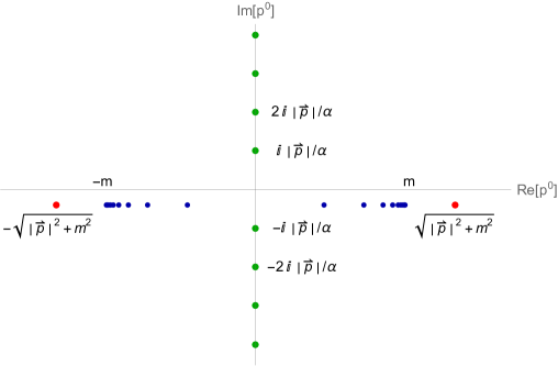
We will show that in order to enforce retarded boundary conditions we must place these bound state poles (201) below the real $p^{0}$ axis. The last set of poles are the usual onshell $p^{2}=m^{2}$ poles in (199), which as per usual we place below the real $p^{0}$ axis to enforce retarded boundary conditions. These are all of the poles of the Green’s function integrand. We plot these poles in Fig.1.

Figure 1: All of the poles of the integrand of the retarded Coulomb Greens function (197) in the complex $p^{0}$-plane. The continuum wavefunctions $v_{l}$ contribute a factor of $\left|\Gamma\left(1+ip^{0}/|\vec{p}|\right)\right|^{2}$ which give rise to simple poles along the imaginary axis $p^{0}=in|\vec{p}|/\alpha$, $n\in\mathbb{N}_{\neq 0}$ indicated in green. The denominator of the bound state’s contribution to the Greens function (198) gives rise to poles at $p^{0}=\pm m/\sqrt{1+\frac{\alpha^{2}}{n^{2}}}$ indicated in blue. We place these bound state poles below the real axis to enforce retarded boundary conditions. The denominator of the continuum contribution to the Greens function contains two onshell poles indicated in red, which we place below the real axis in order to impose retarded boundary conditions.

Cancellation of bound state poles

In order for the Green’s function to satisfy retarded boundary conditions $G(x,y)\propto\theta(x^{0}-y^{0})$, it must be the case that the bound state poles in $I_{C}^{+}$ (200) in the upper-half-plane (UHP) must be cancelled out when including all contributions to the Green’s function. In this section we show that a certain part of the bound state contribution to the Green’s function $I_{B}$ (198) does indeed cancel these poles.

Let us perform the $p^{0}$ integral in the continiuum contribution to the Greens function $I_{C}^{+}$ (199). We consider the case $y^{0}>x^{0}$ first, in which case we close the $p^{0}$ integration contour in the UHP. The additional arc at infinity gives a zero contribution as the asymptotics are still dictated by the $e^{-ip^{0}(x^{0}-y^{0})}$ factor. The integral is therefore given by the sum of the residues of the poles in the UHP. These poles arise from the Gamma functions in $v_{l}$ and have the following residue at the location of the pole

$$\underset{p^{0}\rightarrow i\frac{|\vec{p}|}{|\alpha|}n}{\text{Res}}\Gamma\Bigg{(}1+l+i\alpha\frac{p^{0}}{|\vec{p}|}\Bigg{)}\Gamma\Bigg{(}1+l-i\alpha\frac{p^{0}}{|\vec{p}|}\Bigg{)}=i\frac{|\vec{p}|}{|\alpha|}(-1)^{n-l}\frac{(l+n)!}{(n-l-1)!}$$ (202)

where we put absolute value brackets on $\alpha$ so we can simultaneously discuss $\alpha>0$ and $\alpha<0$. Picking up all of these poles in (199) and recalling the definition of the $v_{l}$’s (183), and performing some simplifications we find

$$I_{C}(x,y)\Big{|}_{y^{0}>x^{0}}=(-1)^{l+1}\frac{4}{|\alpha|}\sum_{n=l+1}^{\infty}\frac{(l+n)!(4rr^{\prime})^{l}}{(n-l-1)!\big{[}(2l+1)!\big{]}^{2}}\int_{0}^{\infty}\mathrm{d}|\vec{p}||\vec{p}|^{3+2l}e^{-i|\vec{p}|(|r_{x}|+|r_{y}|)}$$

$$e^{n\frac{|\vec{p}|}{|\alpha|}(x^{0}-y^{0})}\frac{{}_{1}F_{1}\Big{(}1+l+s(\alpha)n,2l+2;2i|\vec{p}|r_{x}\Big{)}{}_{1}F_{1}\Big{(}1+l+s(\alpha)n,2l+2;2i|\vec{p}|r_{y}\Big{)}}{m^{2}+|\vec{p}|^{2}\Big{(}1+\frac{n^{2}}{\alpha^{2}}\Big{)}}$$ (203)

where the $s(\alpha)\coloneqq\text{sign}(\alpha)$ arises in the first argument of the ${}_{1}F_{1}$’s due to $-i\alpha\frac{p^{0}}{|\vec{p}|}\Big{|}_{p^{0}\rightarrow i\frac{|\vec{p}|}{|\alpha|}n}=s(\alpha)n$. Note that we used the relation

$${}_{1}F_{1}(a,b,-z)=e^{-z}{}_{1}F_{1}(b-a,b,z)$$ (204)

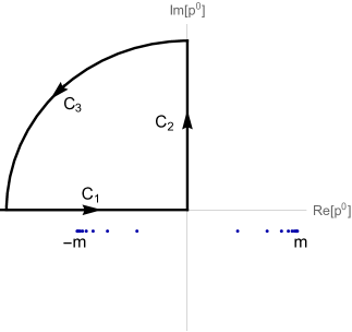
to make the signs of the arguments of the confluent hypergeometrics and the argument of the exponential radial functions the same. We now demonstrate that (203) is precisely cancelled by the $I_{B}$ contribution for $y^{0}>x^{0}$, thus ensuring retarded boundary conditions. The $\theta(-\alpha p^{0})$ theta function in $I_{B}$ implies that the $p^{0}$ only runs along half of the real line, and the sign of the half-line depends on the sign of $\alpha$. We will deform the contour as indicated in Fig.2. The arc at infinity gives a zero contribution due to the $e^{-ip^{0}(x^{0}-y^{0})}$ determining the asymptotics. Implementing the deformation described in Fig.2 we find

Figure 2: Contour deformation for $\alpha>0$ and $y^{0}>x^{0}$ for the $I_{B}$ integrand (198), justifying the replacement to (205). The original integration contour is $C_{1}$. Because there is no pole enclosing the indicated quarter circle we have that $C_{1}=-C_{2}-C_{3}$. Because $C_{3}=0$ we conclude that $C_{1}=-C_{2}$. For $\alpha<0$ the original integration contour $C_{1}^{\prime}$ would instead be the half-line along the positive real axis $p^{0}>0$. Applying the same contour deforming argument we conclude that we again obtain $C_{2}$, but with the opposite orientation than before $C_{1}^{\prime}=C_{2}$.

$$I_{B}=-\text{sign}(\alpha)\sum_{n=l+1}^{\infty}\int_{0}^{i\infty}\mathrm{d}p^{0}e^{-ip^{0}(x^{0}-y^{0})}\frac{\rho_{nl}\Big{(}r_{x},\frac{1}{\alpha p^{0}}\Big{)}\rho^{\star}_{nl}\Big{(}r_{y},\frac{1}{\alpha p^{0}}\Big{)}}{m^{2}-\Big{(}1+\frac{\alpha^{2}}{n^{2}}\Big{)}(p^{0})^{2}}$$ (205)

where the integration contour is straight upwards along the imaginary $p^{0}$ axis. For each $n$ we change to new a integration variable from $p^{0}$ to $|\vec{p}|$, where

$$p^{0}=\frac{in}{|\alpha|}|\vec{p}|$$ (206)

This gives us

$$I_{B}=-\text{sign}(\alpha)\sum_{n=l+1}^{\infty}\frac{in}{|\alpha|}\int_{0}^{\infty}\mathrm{d}|\vec{p}|e^{\frac{n|\vec{p}|}{|\alpha|}(x^{0}-y^{0})}\frac{\rho_{nl}\Big{(}r_{x},in|\vec{p}|s(\alpha)\Big{)}\rho^{\star}_{nl}\Big{(}r_{y},in|\vec{p}|s(\alpha)\Big{)}}{m^{2}+\Big{(}1+\frac{n^{2}}{\alpha^{2}}\Big{)}|\vec{p}|^{2}}$$ (207)

where $s(\alpha)=\frac{\alpha}{|\alpha|}=\text{sign}(\alpha)$. Plugging in the expression for $\rho$, (184) and simplifying we find

$$I_{B}=(-1)^{l}\frac{4}{|\alpha|}\frac{1}{[(2l+1)!]^{2}}\sum_{n=l+1}^{\infty}\frac{(n+l)!}{(n-l-1)!}\left(4rr^{\prime}\right)^{l}\int_{0}^{\infty}\mathrm{d}|\vec{p}|\,\,|\vec{p}|^{2l+3}e^{\frac{n|\vec{p}|}{\alpha}|(x^{0}-y^{0})}$$

$$e^{-is(\alpha)|\vec{p}|(r+r^{\prime})}\frac{{}_{1}F_{1}\Big{(}l+1-n,2l+2,2is(\alpha)|\vec{p}|r\Big{)}{}_{1}F_{1}\Big{(}l+1-n,2l+2,2is(\alpha)|\vec{p}|r^{\prime}\Big{)}}{m^{2}+\Big{(}1+\frac{n^{2}}{\alpha^{2}}\Big{)}|\vec{p}|^{2}}$$ (208)

which upon using (204) to shift the $s(\alpha)$ from the third argument of the ${}_{1}F_{1}$’s to the first argument and the radial exponential factor, precisely cancels (203). We therefore have that the retarded Green’s function with the placement of the poles as in 1 does indeed satisfy retarded boundary conditions $G^{+}(x,y)\propto\theta(x^{0}-y^{0})$.

The $x^{0}>y^{0}$ case

For evaluating the $p^{0}$ integral in $I_{C}^{+}$ (203) for the case $x^{0}>y^{0}$, we can add an arc at infinity in the lower-half plane as this arc gives a zero contribution due to the $e^{-i(x^{0}-y^{0})}$ factor determine the asymptotics. We therefore have that $I_{C}^{+}$ for $x^{0}>y^{0}$ is given by the sum of its residues in the lower-half-plane (LHP). These are the green ($p^{0}=-in\frac{|\vec{p}|}{|\alpha|}$) and red ($p^{2}=m^{2}$ on-shell) poles in Fig.1. For the half-line integral in the bound-states’ contribution (198), we again perform a contour deformation this time using a quarter-circle in the LHP, analogous to Fig. (2). Doing so, we obtain a half-line contribution running along the imaginary $p^{0}$-axis, but in addition, we also pick up the bound state poles $(p^{0})^{2}=m^{2}/(1+\frac{\alpha^{2}}{n^{2}})$ indicated in blue in Fig.2. As before, the green poles in $I_{C}^{+}$ are cancelled by the half-line running along the imaginary $p^{0}$ axis in $I_{B}$. The remaining contribution then are the poles $p^{2}=m^{2}$ in $I_{C}^{+}$, and the bound state poles (blue). We now calculate the residue’s on these two set’s of poles.

The residue on these poles are as follows. Consider the residue of the denominator term of the bound state integrand (198) first

$$\underset{p^{0}\rightarrow\pm\frac{m}{\sqrt{1+\frac{\alpha^{2}}{n^{2}}}}}{\text{Res}}\frac{1}{m^{2}-\Big{(}1+\frac{\alpha^{2}}{n^{2}}\Big{)}(p^{0})^{2}} =\mp\frac{1}{2m}\frac{1}{\sqrt{1+\frac{\alpha^{2}}{n^{2}}}}$$ (209)

$$=\text{sign}(\alpha)\frac{|E_{n}|}{2m^{2}}$$ (210)

The pole we pick up is dictated by the sign of $\alpha$. If $\alpha$ is positive then we pick up the positive poles, and visa versa. The orientation is clockwise for both is clockwise, thus giving a factor of $-(2\pi i)$. Altogether the bound state contribution is given purely in terms of its onshell expansion

$$G^{+}_{B}(x,y)=i\,\theta(x^{0}-y^{0})\sum_{l=0}^{\infty}\sum_{n=l+1}^{\infty}\sum_{m=-l}^{l}E_{n}\phi_{nlm}(x)\phi^{\star}_{nlm}(y)$$ (211)

where we returned to the form (197) where we include the multiplication by the spherical harmonics, we used that there is a factor of $\sqrt{2}m$ between the NRQM wavefunctions and the relativistic ones (185), and we used that when the energy is on-shell we obtain the $\phi_{nlm}$’s. Next we look at the continuum contribution $I_{C}^{+}$. As we have demonstrated that the gamma function poles cancel, so we can return to the form (180)

$$G^{+}_{C}(x,y)=-\int\frac{\mathrm{d}^{4}p}{(2\pi)^{4}}\,\,\frac{\chi_{\text{in/out}}(x,p,u_{s})\chi_{\text{in/out}}^{\star}(y,p,u_{s})}{p^{2}-m^{2}\pm i\epsilon}$$ (212)

and pick up only the $p^{2}=m^{2}$ onshell poles, to obtain

$$G^{++}_{C}(x,y)=i\theta(x^{0}-y^{0})\int\frac{\mathrm{d}^{3}p}{(2\pi)^{3}}\frac{1}{2E_{p}}\Bigg{(}\phi_{\text{in/out}}(x,p,u_{s})\phi_{\text{in/out}}^{\star}(y,p,u_{s})-(E_{p}\rightarrow-E_{p})\Bigg{)}$$ (213)

where we have added an additional plus sign to the superscript as this is not strictly equal to $G^{+}$, due to the required addition of the bound state off-shell Green’s function to enact the cancellation of the Gamma function poles. Altogether we have

$$G^{+}(x,y)=i\, \theta(x^{0}-y^{0})\Bigg{\{}\sum_{l=0}^{\infty}\sum_{n=l+1}^{\infty}\sum_{m=-l}^{l}E_{n}\phi_{nlm}(x)\phi^{\star}_{nlm}(y)$$

$$+\int\frac{\mathrm{d}^{3}p}{(2\pi)^{3}}\frac{1}{2E_{p}}\Big{(}\phi_{\text{in/out}}(x,p,u_{s})\phi_{\text{in/out}}^{\star}(y,p,u_{s})-(E_{p}\rightarrow-E_{p})\Big{)}\Bigg{\}}$$ (214)

For the case of the advanced Green’s function the argument of the theta function changes sign, and we obtain an overall minus sign due to the change in orientation when picking up the on-shell residues.

C.4 Vanishing of equal time retarded Green’s function

Following Hostler hostler1964coulomb Eq. 2.12-2.16 we will show that the retarded Green’s function vanishes at equal times

$$\delta(x^{0}-y^{0})\Bigg{\{} \sum_{l=0}^{\infty}\sum_{n=l+1}^{\infty}\sum_{m=-l}^{l}E_{n}\phi_{nlm}(x)\phi^{\star}_{nlm}(y)$$

$$\int\frac{\mathrm{d}^{3}p}{(2\pi)^{3}2E_{p}}\Bigg{(}\phi_{\text{in/out}}(p,x)\phi^{\star}_{\text{in/out}}(p,y)-(E_{p}\rightarrow-E_{p})\Bigg{)}\Bigg{\}}=0$$ (215)

Hostler considered the Green’s function in the partial wave basis, and furthermore considered the solutions of the full-SQED equations of motion. For ease of reference, and to adapt the proof to our conventions for the normalization of the states, we reproduce their proof with minor modifications here.

Assuming, without proof, that the continuum and bound state solutions form a complete basis for the solution space to the semi-free EQM, we have that any SQED normalizable solution to the semi-free EQM can be expressed in this basis

$$f(x)= \sum_{l=0}^{\infty}\sum_{n=l+1}^{\infty}\sum_{m=-l}^{l}b_{nlm}E_{n}\phi_{nlm}(x)$$

$$+\int\frac{\mathrm{d}^{3}k}{(2\pi)^{3}2E_{k}}\,\,\Bigg{(}a_{+}(k)\phi_{\text{in/out}}(k,x)-a_{-}(k)\phi_{\text{in/out}}(\vec{k},-E_{k},x)\Bigg{)},$$ (216)

where the coefficients can be extracted using the orthogonality (43, 175) of the basis functions

$$b(n,l,m)=\braket{\phi_{nlm}}{f}_{\text{SQED}}\qquad a_{\pm}(k)=\big{\langle}\phi_{\text{in/out}}(k,\pm E_{k})\big{|}f\big{\rangle}_{\text{SQED}}.$$ (217)

The measure in (216) is chosen so as to compensate for the norm of the states. Let us consider the expansion 216 at time $t=0$, and use the explicit expressions for the expansion coefficients

$$f(\vec{x},t=0)=\Bigg{[}\sum_{l=0}^{\infty}\sum_{n=l+1}^{\infty}\sum_{m=-l}^{l}E_{n}\int\mathrm{d}^{3}y\phi_{nlm}(x)\phi_{nlm}^{\star}(y)\Bigg{(}i\dot{f}(\vec{y},0)+\Big{(}iE_{n}-\frac{\alpha}{r}\Big{)}f(\vec{y},0)\Bigg{)}$$

$$+\int\frac{\mathrm{d}^{3}y\,\mathrm{d}^{3}k}{(2\pi)^{3}2E_{k}}\phi_{\text{in/out}}(k,x)\phi^{\star}_{\text{in/out}}(k,y)\Bigg{(}i\dot{f}(\vec{y},0)+\Big{(}iE_{k}-\frac{\alpha}{r}\Big{)}f(\vec{y},0)\Bigg{)}$$

$$-\int\frac{\mathrm{d}^{3}y\,\mathrm{d}^{3}k}{(2\pi)^{3}2E_{k}}\phi^{-E_{k}}_{\text{in/out}}(k,x)\phi^{\star,-E_{k}}_{\text{in/out}}(k,y)\Bigg{(}i\dot{f}(\vec{y},0)+\Big{(}-i|E_{k}|-\frac{\alpha}{r}\Big{)}f(\vec{y},0)\Bigg{)}\Bigg{]}\Bigg{|}_{x^{0}=y^{0}=0}.$$ (218)

Now, because the SQED EQM are second-order in time we have the $f(\vec{x},0)$ can be arbitrarily prescribed independent of $\dot{f}(\vec{x},0)$. Thus $\dot{f}$ must drop out of (218). To make this argument precise, choose $f(\vec{x},0)=0$ in (218), which gives us an entire function space of identities relating the $\phi$’s, one for each choice of $\dot{f}(\vec{y},0)$. These relations can only be satisfied if the co-efficient of $\dot{f}(\vec{y},0)$ in (218) vanishes at each point in $y-$space, namely

$$\delta(x^{0}-y^{0}) \Bigg{[}\sum_{l=0}^{\infty}\sum_{n=l+1}^{\infty}\sum_{m=-l}^{l}E_{n}\phi_{nlm}(x)\phi_{nlm}^{\star}(y)$$

$$+\int\frac{\mathrm{d}^{3}k}{(2\pi)^{3}2E_{k}}\phi_{\text{in/out}}(k,x)\phi^{\star}_{\text{in/out}}(k,y)-\phi^{-E_{k}}_{\text{in/out}}(k,x)\phi^{\star,-E_{k}}_{\text{in/out}}(k,y)\Bigg{]}=0,$$ (219)

which is what we sought to prove (215). Now that we have established that the $\dot{f}(\vec{y},0)$ term drops out of (218) we can also derive a completeness relation. Note that the $\frac{\alpha}{r}$ terms in (218) also vanish on account of (219). Now as $f(\vec{x},0)$ occurs on the LHS and RHS of (218) it must be the case that the integration over $\vec{k}$-space of the coefficients of $f(\vec{y},0)$ for the remaining terms on the RHS must be $\delta^{3}(\vec{x}-\vec{y})$,

$$i\,\delta(x^{0}-y^{0})\Bigg{[}\sum_{l=0}^{\infty}\sum_{n=l+1}^{\infty}\sum_{m=-l}^{l}E^{2}_{n}\phi_{nlm}(x)\phi_{nlm}^{\star}(y)$$

$$+\frac{1}{2}\int\frac{\mathrm{d}^{3}k}{(2\pi)^{3}}\Bigg{(}\phi_{\text{in/out}}(k,x)\phi^{\star}_{\text{in/out}}(k,y)+\phi^{-E_{k}}_{\text{in/out}}(k,x)\phi^{\star,-E_{k}}_{\text{in/out}}(k,y)\Bigg{)}\Bigg{]}=\delta^{4}(x-y)$$ (220)

which indicates the completeness of the continiuum and bound states. The argument which lead to (220) is circular as we assumed without proof the completeness of the bound state and continuum solutions at (216), and then consistently concluded that the states form a complete set. We consider the completeness assumption to be reasonable, and it is nevertheless useful to have the expected form of the completeness relation (220) presented for future works that may prove the completeness relation by other means.

References

- (1) F. Bloch and A. Nordsieck, Note on the Radiation Field of the electron, Phys. Rev. 52 (1937) 54–59.
- (2) P. P. Kulish and L. D. Faddeev, Asymptotic conditions and infrared divergences in quantum electrodynamics, Theor. Math. Phys. 4 (1970) 745.
- (3) J. D. Dollard, Asymptotic convergence and the coulomb interaction, Journal of Mathematical Physics 5 (1964) 729–738.
- (4) T. W. B. Kibble, Coherent Soft-Photon States and Infrared Divergences. I. Classical Currents, J. Math. Phys. 9 (1968), no. 2 315–324.
- (5) V. Chung, Infrared Divergence in Quantum Electrodynamics, Phys. Rev. 140 (1965) B1110–B1122.
- (6) H. Hannesdottir and M. D. Schwartz, -Matrix for massless particles, Phys. Rev. D 101 (2020), no. 10 105001, [arXiv:1911.06821].
- (7) H. Hannesdottir and M. D. Schwartz, Finite matrix, Phys. Rev. D 107 (2023), no. 2 L021701, [arXiv:1906.03271].
- (8) D. A. Forde and A. Signer, Infrared finite amplitudes for massless gauge theories, Nucl. Phys. B 684 (2004) 125–161, [hep-ph/0311059].
- (9) I.-J. Kang and L. M. Brown, Higher born approximations for the coulomb scattering of a spinless particle, Physical Review 128 (1962), no. 6 2828.
- (10) O. Steinmann, Über den Zusammenhang Zwischen den Wightmanfunktionen und den Retardierten Kommutatoren, Helvetica Physica Acta 33 (1960) 257–298.
- (11) J. L. Bourjaily, H. Hannesdottir, A. J. McLeod, M. D. Schwartz, and C. Vergu, Sequential Discontinuities of Feynman Integrals and the Monodromy Group, JHEP 01 (2021) 205, [arXiv:2007.13747].
- (12) C. Fevola, S. Mizera, and S. Telen, Principal Landau Determinants, arXiv:2311.16219.
- (13) M. Berghoff and E. Panzer, Hierarchies in relative Picard-Lefschetz theory, arXiv:2212.06661.
- (14) H. S. Hannesdottir, A. J. McLeod, M. D. Schwartz, and C. Vergu, Constraints on sequential discontinuities from the geometry of on-shell spaces, JHEP 07 (2023) 236, [arXiv:2211.07633].
- (15) C. de Rham, S. Kundu, M. Reece, A. J. Tolley, and S.-Y. Zhou, Snowmass White Paper: UV Constraints on IR Physics, in Snowmass 2021, 3, 2022. arXiv:2203.06805.
- (16) M. Kruczenski, J. Penedones, and B. C. van Rees, Snowmass White Paper: S-matrix Bootstrap, arXiv:2203.02421.
- (17) S. Caron-Huot, L. J. Dixon, J. M. Drummond, F. Dulat, J. Foster, Ömer Gürdoğan, M. von Hippel, A. J. McLeod, and G. Papathanasiou, The steinmann cluster bootstrap for n=4 super yang-mills amplitudes, 2020.
- (18) D. R. Yennie, S. C. Frautschi, and H. Suura, The infrared divergence phenomena and high-energy processes, Annals of Physics 13 (June, 1961) 379–452.
- (19) S. Weinberg, Infrared photons and gravitons, Phys. Rev. 140 (1965) B516–B524.
- (20) S. Weinberg, The Quantum theory of fields. Vol. 1: Foundations. Cambridge University Press, 6, 2005.
- (21) D. Zwanziger, Reduction formulas for charged particles and coherent states in quantum electrodynamics, Phys. Rev. D 7 (Feb, 1973) 1082–1099.
- (22) B. Sahoo and A. Sen, Classical and quantum results on logarithmic terms in the soft theorem in four dimensions, Journal of High Energy Physics 2019 (feb, 2019).
- (23) H. Hirai, Towards Infrared Finite S-matrix in Quantum Field Theory. PhD thesis, Aff1= Natural Science Education, National Institute of Technology, Kisarazu College, Kisarazu, Japan, GRID:grid.459759.3, Osaka U., Inst. Phys., 2021.
- (24) S. Duary, AdS correction to the Faddeev-Kulish state: migrating from the flat peninsula, JHEP 05 (2023) 079, [arXiv:2212.09509].
- (25) S. Duary, E. Hijano, and M. Patra, Towards an IR finite S-matrix in the flat limit of AdS/CFT, arXiv:2211.13711.
- (26) E. Hijano and D. Neuenfeld, Soft photon theorems from CFT Ward identites in the flat limit of AdS/CFT, JHEP 11 (2020) 009, [arXiv:2005.03667].
- (27) X. Feal, A. Tarasov, and R. Venugopalan, QED as a many-body theory of worldlines: General formalism and infrared structure, Phys. Rev. D 106 (2022), no. 5 056009, [arXiv:2206.04188].
- (28) X. Feal, A. Tarasov, and R. Venugopalan, QED as a many-body theory of worldlines. II. All-order S-matrix formalism, Phys. Rev. D 107 (2023), no. 9 096021, [arXiv:2211.15712].
- (29) D. Bonocore, Asymptotic dynamics on the worldline for spinning particles, JHEP 02 (2021) 007, [arXiv:2009.07863].
- (30) K. Prabhu, G. Satishchandran, and R. M. Wald, Infrared finite scattering theory in quantum field theory and quantum gravity, Phys. Rev. D 106 (2022), no. 6 066005, [arXiv:2203.14334].
- (31) N. Agarwal, L. Magnea, C. Signorile-Signorile, and A. Tripathi, The infrared structure of perturbative gauge theories, Phys. Rept. 994 (2023) 1–120, [arXiv:2112.07099].
- (32) M. Rai, L. Chen, and D. Boyanovsky, Infrared dressing in real time: emergence of anomalous dimensions, Phys. Rev. D 104 (2021) 085021, [arXiv:2105.06572].
- (33) H. Hirai and S. Sugishita, IR finite S-matrix by gauge invariant dressed states, JHEP 02 (2021) 025, [arXiv:2009.11716].
- (34) H. Furugori and S. Nojiri, Dressed asymptotic states and QED infrared physics, Phys. Rev. D 104 (2021), no. 12 125004, [arXiv:2007.02518].
- (35) J. Ware, R. Saotome, and R. Akhoury, Construction of an asymptotic s matrix for perturbative quantum gravity, Journal of High Energy Physics 2013 (oct, 2013).
- (36) H. Hirai and S. Sugishita, Dress code for infrared safe scattering in QED, PTEP 2023 (2023), no. 5 053B04, [arXiv:2209.00608].
- (37) R. Gonzo, T. McLoughlin, and A. Puhm, Celestial holography on Kerr-Schild backgrounds, JHEP 10 (2022) 073, [arXiv:2207.13719].
- (38) S. Pasterski, A comment on loop corrections to the celestial stress tensor, JHEP 01 (2023) 025, [arXiv:2205.10901].
- (39) K. Nguyen, A. Rios Fukelman, and C. D. White, Celestial soft dressings from generalised Wilson lines, arXiv:2304.01250.
- (40) S. Choi and R. Akhoury, BMS Supertranslation Symmetry Implies Faddeev-Kulish Amplitudes, JHEP 02 (2018) 171, [arXiv:1712.04551].
- (41) L. Freidel, D. Pranzetti, and A.-M. Raclariu, A discrete basis for celestial holography, arXiv:2212.12469.
- (42) H. Krishna and B. Sahoo, Universality of Loop Corrected Soft Theorems in 4d, arXiv:2308.16807.
- (43) D. Kapec and P. Mitra, Shadows and soft exchange in celestial CFT, Phys. Rev. D 105 (2022), no. 2 026009, [arXiv:2109.00073].
- (44) N. Kalyanapuram, Infrared and Holographic Aspects of the -Matrix in Gauge Theory and Gravity, arXiv:2107.06660.
- (45) K. Nguyen and J. Salzer, Celestial IR divergences and the effective action of supertranslation modes, JHEP 09 (2021) 144, [arXiv:2105.10526].
- (46) L. Magnea, Non-abelian infrared divergences on the celestial sphere, JHEP 05 (2021) 282, [arXiv:2104.10254].
- (47) N. Arkani-Hamed, M. Pate, A.-M. Raclariu, and A. Strominger, Celestial amplitudes from UV to IR, JHEP 08 (2021) 062, [arXiv:2012.04208].
- (48) T. He and P. Mitra, Covariant Phase Space and Soft Factorization in Non-Abelian Gauge Theories, JHEP 03 (2021) 015, [arXiv:2009.14334].
- (49) S. Atul Bhatkar, Ward identity for loop level soft photon theorem for massless QED coupled to gravity, JHEP 10 (2020) 110, [arXiv:1912.10229].
- (50) D. Kapec, M. Perry, A.-M. Raclariu, and A. Strominger, Infrared Divergences in QED, Revisited, Phys. Rev. D 96 (2017), no. 8 085002, [arXiv:1705.04311].
- (51) A. Ashtekar, Geometry and Physics of Null Infinity, arXiv:1409.1800.
- (52) B. Gabai and A. Sever, Large gauge symmetries and asymptotic states in QED, JHEP 12 (2016) 095, [arXiv:1607.08599].
- (53) S. Choi, U. Kol, and R. Akhoury, Asymptotic Dynamics in Perturbative Quantum Gravity and BMS Supertranslations, JHEP 01 (2018) 142, [arXiv:1708.05717].
- (54) X.-L. Su, A. Hamma, and A. Marciano, Scrambling Power of Soft Photons, arXiv:2304.12277.
- (55) X.-L. Su, A. Hamma, and A. Marciano, On the irrelevance of the scrambling power of gravity for black hole radiation, arXiv:2304.12278.
- (56) A. Irakleous, T. N. Tomaras, and N. Toumbas, Soft photon radiation and entanglement, Eur. Phys. J. C 81 (2021), no. 8 745, [arXiv:2105.11858].
- (57) M. Mirbabayi and M. Porrati, Dressed Hard States and Black Hole Soft Hair, Phys. Rev. Lett. 117 (2016), no. 21 211301, [arXiv:1607.03120].
- (58) R. Bousso and M. Porrati, Soft Hair as a Soft Wig, Class. Quant. Grav. 34 (2017), no. 20 204001, [arXiv:1706.00436].
- (59) A. Strominger, Black Hole Information Revisited, arXiv:1706.07143.
- (60) C. Csáki, Z.-Y. Dong, O. Telem, J. Terning, and S. Yankielowicz, Dressed vs. pairwise states, and the geometric phase of monopoles and charges, JHEP 02 (2023) 211, [arXiv:2209.03369].
- (61) J. Mund, K.-H. Rehren, and B. Schroer, Infraparticle quantum fields and the formation of photon clouds, JHEP 04 (2022) 083, [arXiv:2109.10342].
- (62) W. Donnelly and S. B. Giddings, Diffeomorphism-invariant observables and their nonlocal algebra, Phys. Rev. D 93 (2016), no. 2 024030, [arXiv:1507.07921]. [Erratum: Phys.Rev.D 94, 029903 (2016)].
- (63) P. Di Vecchia, C. Heissenberg, R. Russo, and G. Veneziano, Classical gravitational observables from the Eikonal operator, Phys. Lett. B 843 (2023) 138049, [arXiv:2210.12118].
- (64) S. Nabeebaccus and R. Zwicky, Resolving charged hadrons in QED — gauge invariant interpolating operators, JHEP 11 (2022) 101, [arXiv:2209.06925].
- (65) S. Biswas and G. W. Semenoff, Soft scalars do not decouple, Phys. Rev. D 106 (2022), no. 10 105023, [arXiv:2208.05023].
- (66) D. Bhamre and A. Misra, Infrared divergences in e+e-→2 jets in the light front coherent state formalism, Phys. Rev. D 107 (2023), no. 1 014001, [arXiv:2206.06933].
- (67) A. Cristofoli, R. Gonzo, N. Moynihan, D. O’Connell, A. Ross, M. Sergola, and C. D. White, The Uncertainty Principle and Classical Amplitudes, arXiv:2112.07556.
- (68) L. Berezhiani, G. Dvali, and O. Sakhelashvili, de Sitter space as a BRST invariant coherent state of gravitons, Phys. Rev. D 105 (2022), no. 2 025022, [arXiv:2111.12022].
- (69) D. Boyanovsky, M. Rai, and L. Chen, Ultralight dark matter or dark radiation cosmologically produced from infrared dressing, Phys. Rev. D 104 (2021), no. 12 123552, [arXiv:2110.15488].
- (70) A. Addazi and K. A. Zeng, Soft gravitational radiation from multi-body collisions, JHEP 11 (2021) 193, [arXiv:2110.01194].
- (71) C. DeLisle and P. C. E. Stamp, Decoherence of a 2-Path System by Infrared Photons, arXiv:2211.05813.
- (72) C. Gaß, K.-H. Rehren, and F. C. Tippner, On the spacetime structure of infrared divergencies in QED, Lett. Math. Phys. 112 (2022), no. 2 37, [arXiv:2109.10148].
- (73) S. Kolekar and J. Louko, Can a localised quantum system see soft photons?, arXiv:2108.04278.
- (74) R. Gonzo and A. Pokraka, Light-ray operators, detectors and gravitational event shapes, JHEP 05 (2021) 015, [arXiv:2012.01406].
- (75) M. Ciafaloni, D. Colferai, and G. Veneziano, Infrared features of gravitational scattering and radiation in the eikonal approach, Phys. Rev. D 99 (2019), no. 6 066008, [arXiv:1812.08137].
- (76) D. Carney, L. Chaurette, D. Neuenfeld, and G. W. Semenoff, Infrared quantum information, Phys. Rev. Lett. 119 (2017), no. 18 180502, [arXiv:1706.03782].
- (77) A. Addazi, M. Bianchi, and G. Veneziano, Soft gravitational radiation from ultra-relativistic collisions at sub- and sub-sub-leading order, JHEP 05 (2019) 050, [arXiv:1901.10986].
- (78) C. Frye, H. Hannesdottir, N. Paul, M. D. Schwartz, and K. Yan, Infrared Finiteness and Forward Scattering, Phys. Rev. D 99 (2019), no. 5 056015, [arXiv:1810.10022].
- (79) H. A. Bethe and L. C. Maximon, Theory of bremsstrahlung and pair production. i. differential cross section, Phys. Rev. 93 (Feb, 1954) 768–784.
- (80) D. S. Crothers and L. J. Dubé, Continuum distorted wave methods in ion—atom collisions, in Advances In Atomic, Molecular, and Optical Physics (D. Bates and B. Bederson, eds.), vol. 30, pp. 287–337. Academic Press, 1992.
- (81) P. C. Martin and R. J. Glauber, Relativistic theory of radiative orbital electron capture, Phys. Rev. 109 (Feb, 1958) 1307–1325.
- (82) L. D. Landau and E. M. Lifshits, Quantum Mechanics: Non-Relativistic Theory, vol. v.3 of Course of Theoretical Physics. Butterworth-Heinemann, Oxford, 1991. See sections 36, 135, 136, 137.
- (83) I. W. Herbst, On the connectedness structure of the coulomb s-matrix, .
- (84) S. Weinberg, Lectures on Quantum Mechanics. Cambridge University Press, 2 ed., 2015.
- (85) J. Chadwick, The scattering of alpha-particles in helium, Proceedings of the Royal Society of London. Series A, Containing Papers of a Mathematical and Physical Character 128 (1930), no. 807 114–122, [https://royalsocietypublishing.org/doi/pdf/10.1098/rspa.1930.0098].
- (86) R. Barrachina and J. Macek, Scattering of charged particles, Journal of mathematical physics 30 (1989), no. 11 2581–2584.
- (87) D. Zwanziger, Algebraic Calculation of Nonrelativistic Coulomb Phase Shifts, Journal of Mathematical Physics 8 (Sept., 1967) 1858–1860.
- (88) M. Bander and C. Itzykson, Group theory and the hydrogen atom (i), Reviews of modern Physics 38 (1966), no. 2 330.
- (89) M. Bander and C. Itzykson, Group theory and the hydrogen atom (ii), Reviews of Modern Physics 38 (1966), no. 2 346.
- (90) D. Zwanziger, Algebraic calculation of nonrelativistic coulomb phase shifts, Journal of Mathematical Physics 8 (1967), no. 9 1858–1860.
- (91) J. Wu, A. Stahlhofen, L. Biedenharn, and F. Iachello, A group theoretical calculation of the s matrix for the dirac-coulomb problem, Journal of Physics A: Mathematical and General 20 (1987), no. 14 4637.
- (92) A. Stahlhofen, Algebraic solutions of relativistic coulomb problems, Helvetica Physica Acta 70 (1997).
- (93) G. Kerimov, Models with sl (2, c) symmetry and their s-matrices, Journal of Physics A: Mathematical and General 38 (2005), no. 9 1931.
- (94) J. P. Dahl, Physical origin of the runge-lenz vector, Journal of Physics A: Mathematical and General 30 (1997), no. 19 6831.
- (95) S. Caron-Huot and J. M. Henn, Solvable Relativistic Hydrogenlike System in Supersymmetric Yang-Mills Theory, Phys. Rev. Lett. 113 (2014), no. 16 161601, [arXiv:1408.0296].
- (96) J. Alvarez-Jimenez, I. Cortese, J. A. García, D. Gutiérrez-Ruiz, and J. D. Vergara, Relativistic Runge-Lenz vector: from SYM to SO(4) scalar field theory, JHEP 10 (2018) 153, [arXiv:1805.12165].
- (97) A. Barut and W. Rasmussen, The hydrogen atom as a relativistic elementary particle. ii. relativistic scattering problems and photo-effect, Journal of Physics B: Atomic and Molecular Physics 6 (1973), no. 9 1713.
- (98) A. Barut and W. Rasmussen, The hydrogen atom as a relativistic elementary particle. ii. relativistic scattering problems and photo-effect, Journal of Physics B: Atomic and Molecular Physics 6 (1973), no. 9 1713.
- (99) A. Barut and W. Rasmussen, Nonrelativistic and relativistic coulomb amplitude as the matrix element of a rotation in o (4, 2), Physical Review D 3 (1971), no. 4 956.
- (100) A. Barut, W. Rasmussen, and S. Salamó, Relativistic transition amplitudes in a class of o (4, 2) infinite multiplets. i. continuum-continuum transitions, Physical Review D 10 (1974), no. 2 622.
- (101) B. S. DeWitt, Quantum theory of gravity. ii. the manifestly covariant theory, Phys. Rev. 162 (Oct, 1967) 1195–1239.
- (102) I. Y. Arefeva, L. D. Faddeev, and A. A. Slavnov, Generating Functional for the s Matrix in Gauge Theories, Teor. Mat. Fiz. 21 (1974) 311–321.
- (103) L. Abbott, M. Grisaru, and R. Schaefer, The background field method and the s-matrix, Nuclear Physics B 229 (1983), no. 2 372–380.
- (104) A. Jevicki and C. Lee, S-matrix generating functional and effective action, Phys. Rev. D 37 (Mar, 1988) 1485–1491.
- (105) A. Rosly and K. Selivanov, On amplitudes in the self-dual sector of yang-mills theory, Physics Letters B 399 (Apr., 1997) 135–140.
- (106) A. Rosly and K. Selivanov, Gravitational sd perturbiner, 1997.
- (107) K. G. Selivanov, Post-classicism in tree amplitudes, 1999.
- (108) S. Mizera and B. Skrzypek, Perturbiner methods for effective field theories and the double copy, Journal of High Energy Physics 2018 (Oct., 2018).
- (109) L. M. Garozzo, L. Queimada, and O. Schlotterer, Berends-giele currents in bern-carrasco-johansson gauge for f3- and f4-deformed yang-mills amplitudes, Journal of High Energy Physics 2019 (Feb., 2019).
- (110) A. Ilderton and W. Lindved, Scattering amplitudes and electromagnetic horizons, 2023.
- (111) T. Adamo, A. Cristofoli, and P. Tourkine, Eikonal amplitudes from curved backgrounds, SciPost Physics 13 (Aug., 2022).
- (112) L. Hostler, Coulomb Green’s Functions and the Furry Approximation, Journal of Mathematical Physics 5 (May, 1964) 591–611.
- (113) J. Schwinger, Coulomb Green’s Function, J. Math. Phys. 5 (1964) 1606–1608.
- (114) J. C. Chen and A. C. Chen, Nonrelativistic off-shell two-body coulomb amplitudes, Advan. At. Mol. Phys., v. 8, pp. 71-129 (1, 1972).
- (115) S. S. Vasan and M. Seetharaman, The coulomb green’s function revisited, Pramana 45 (1995), no. 2 165–174.
- (116) K. Mano, Eigenfunction form of the nonrelativistic coulomb green’s function, Journal of Mathematical Physics 4 (1963), no. 4 522–529.
- (117) K. Mano, Representations for the nonrelativistic coulomb green’s function, Journal of Mathematical Physics 5 (1964), no. 4 505–508.
- (118) J. D. Dollard, Quantum-mechanical scattering theory for short-range and coulomb interactions, The Rocky Mountain Journal of Mathematics (1971) 5–88.
- (119) J. R. Taylor, A new rigorous approach to coulomb scattering, Il Nuovo Cimento B (1971-1996) 23 (1974), no. 2 313–334.
- (120) Q. gui Lin, On the partial wave amplitude of coulomb scattering in three dimensions, American Journal of Physics 68 (nov, 2000) 1056–1057.
- (121) S.-L. Li, Y.-Y. Liu, W.-D. Li, and W.-S. Dai, Eliminating oscillation in partial sum approximation of periodic function, 2021.
- (122) N. F. Mott and R. H. Fowler, The polarisation of electrons by double scattering, Proceedings of the Royal Society of London. Series A, Containing Papers of a Mathematical and Physical Character 135 (1932), no. 827 429–458, [https://royalsocietypublishing.org/doi/pdf/10.1098/rspa.1932.0044].
- (123) T. Adamo, A. Cristofoli, and P. Tourkine, Eikonal amplitudes from curved backgrounds, SciPost Phys. 13 (2022), no. 2 032, [arXiv:2112.09113].
- (124) D. Kabat and M. Ortiz, Eikonal quantum gravity and planckian scattering, Nuclear Physics B 388 (dec, 1992) 570–592.
- (125) T. Adamo, G. Bogna, L. Mason, and A. Sharma, Scattering on self-dual Taub-NUT, arXiv:2309.03834.
- (126) A. Strominger, Lectures on the Infrared Structure of Gravity and Gauge Theory, arXiv:1703.05448.
- (127) H. M. Pilkuhn, Relativistic particle physics. Springer Science & Business Media, 2013.
- (128) T. Adamo, A. Cristofoli, A. Ilderton, and S. Klisch, Scattering amplitudes for self-force, arXiv:2307.00431.
- (129) U. Kol, D. O’connell, and O. Telem, The radial action from probe amplitudes to all orders, JHEP 03 (2022) 141, [arXiv:2109.12092].
- (130) M. D. Cooper, R. H. Jeppesen, and M. B. Johnson, Coulomb effects in the klein-gordon equation for pions, Phys. Rev. C 20 (Aug, 1979) 696–704.
- (131) N. F. N. F. Mott and H. Massey, The theory of atomic collisions / by N. F. Mott and H. S. W. Massey. International series of monographs on physics. Clarendon Press, Oxford, third edition. ed., 1965.
- (132) D. Mulherin and I. Zinnes, Coulomb scattering. i. single channel, Journal of Mathematical Physics 11 (1970), no. 4 1402–1408.
- (133) V. B. Berestetskii, E. M. Lifshitz, and L. P. Pitaevskii, Chapter iv - particles in an external field, in Quantum Electrodynamics (V. B. Berestetskii, E. M. Lifshitz, and L. P. Pitaevskii, eds.), pp. 118–158. Butterworth-Heinemann, Oxford, second edition ed., 1982.
- (134) L. Hostler, Coulomb green’s functions and the furry approximation, Journal of Mathematical Physics 5 (1964), no. 5 591–611.
- (135) A. Nordsieck, Reduction of an integral in the theory of bremsstrahlung, Physical review 93 (1954), no. 4 785.
- (136) N. Saad and R. L. Hall, Integrals containing confluent hypergeometric functions with applications to perturbed singular potentials, Journal of Physics A: Mathematical and General 36 (2003), no. 28 7771.
- (137) F. Colavecchia, G. Gasaneo, and C. Garibotti, Hypergeometric integrals arising in atomic collisions physics, Journal of Mathematical Physics 38 (1997), no. 12 6603–6612.
- (138) M. Gravielle and J. Miraglia, Some nordsieck integrals of interest in radiation and atomic collision theories, Computer physics communications 69 (1992), no. 1 53–58.
- (139) N. F. Mott, The polarisation of electrons by double scattering, Proceedings of the Royal Society of London. Series A, Containing Papers of a Mathematical and Physical Character 135 (1932), no. 827 429–458.
- (140) N. Mukunda, Completeness of the coulomb wave functions in quantum mechanics, Am. J. Phys.;(United States) 46 (1978), no. 9.