Using the effective weak mixing angle as an input parameter in SMEFT

Abstract

We implement electroweak renormalisation schemes involving the effective weak mixing angle to NLO in Standard Model Effective Field Theory (SMEFT). After developing the necessary theoretical machinery, we analyse a select set of electroweak precision observables in such input schemes. An attractive feature is that large corrections from top-quark loops appearing in other schemes are absorbed into the definition of the effective weak mixing angle. On the other hand, the renormalisation condition which achieves this involves a large number of flavour-specific SMEFT couplings between the $Z$ boson and charged leptons, motivating simple flavour assumptions such as minimal flavour violation for practical applications. The results of this paper provide a valuable new component for estimating systematic uncertainties in SMEFT fits by performing analyses in multiple input schemes.

1 Introduction

In the absence of direct new physics discoveries, Standard Model Effective Field Theory (SMEFT) Buchmuller:1985jz ; Wilczek:1977pj ; Grzadkowski:2010es enables to describe in a model-independent fashion small deviations from Standard Model (SM) predictions. SMEFT calculations can be systematically improved by including quantum corrections as well as higher-order terms in the expansion in the new physics scale $\Lambda$. The investigation of next-to-leading order (NLO) corrections in dimension-six SMEFT has been a focus of recent studies. While NLO QCD corrections have been fully automated Degrande:2020evl , NLO electroweak (EW) corrections and, in a few instances next-to-next-to-leading order (NNLO) QCD corrections, have been calculated on a case-by-case basis for specific processes Zhang:2013xya ; Crivellin:2013hpa ; Zhang:2014rja ; Pruna:2014asa ; Grober:2015cwa ; Hartmann:2015oia ; Ghezzi:2015vva ; Hartmann:2015aia ; Gauld:2015lmb ; Aebischer:2015fzz ; Zhang:2016omx ; BessidskaiaBylund:2016jvp ; Maltoni:2016yxb ; Gauld:2016kuu ; Degrande:2016dqg ; Hartmann:2016pil ; Grazzini:2016paz ; deFlorian:2017qfk ; Deutschmann:2017qum ; Baglio:2017bfe ; Dawson:2018pyl ; Degrande:2018fog ; Vryonidou:2018eyv ; Dedes:2018seb ; Grazzini:2018eyk ; Dawson:2018liq ; Dawson:2018jlg ; Dawson:2018dxp ; Neumann:2019kvk ; Dedes:2019bew ; Cullen:2019nnr ; Boughezal:2019xpp ; Dawson:2019clf ; Baglio:2019uty ; Haisch:2020ahr ; Cullen:2020zof ; David:2020pzt ; Dittmaier:2021fls ; Dawson:2021ofa ; Boughezal:2021tih ; Battaglia:2021nys ; Kley:2021yhn ; Faham:2021zet ; Haisch:2022nwz ; Heinrich:2022idm ; Bhardwaj:2022qtk ; Asteriadis:2022ras ; Bellafronte:2023amz ; Kidonakis:2023htm ; Gauld:2023gtb ; Heinrich:2023rsd .

An essential ingredient common to all NLO calculations is the choice of the EW input scheme. In the recent work Biekotter:2023xle , we systematically examined at NLO in SMEFT the commonly employed $\alpha$, $\alpha_{\mu}$, and LEP schemes, which are defined in table 1 and use combinations of the Fermi constant $G_{F}$, the masses of the $W$ and $Z$ bosons, $M_{W}$ and $M_{Z}$, as well as the electromagnetic coupling $\alpha$ as the three independent EW input parameters. This involved cataloguing the set of Wilson coefficients entering finite parts of observables after the cancellation of UV divergences in different schemes, identifying dominant sets of universal corrections associated with contributions from top-quark loops, and providing a methodology for including these scheme-dependent universal NLO corrections in the LO results, thus extending previous discussions of EW input schemes in SMEFT Brivio:2017bnu ; Brivio:2021yjb .

In the SM, several studies have proposed EW input schemes which use the effective leptonic weak mixing angle $\sin\theta_{\text{eff}}^{\ell}$ as an input parameter Kennedy:1988sn ; Renard:1994ay ; Ferroglia:2001cr ; Ferroglia:2002rg ; Chiesa:2019nqb ; Amoroso:2023uux . The effective leptonic weak mixing angle has been measured with per-mille level precision at LEP ALEPH:2005ab , the Tevatron CDF:2018cnj and the LHC ATLAS:2015ihy ; ATLAS:2018gqq ; CMS:2018ktx ; LHCb:2015jyu . Its numerical precision is (more than an order of magnitude) below that of other commonly used input values such as the mass of the $W$ boson. Future experiments, such as the P2 experiment at MESA Berger:2015aaa , as well as the Møller MOLLER:2014iki and SoLID Chen:2014psa ; JeffersonLabSoLID:2022iod experiments at Jefferson Laboratory, will test this quantity with similar precision at lower energy scales.

In spite of the past and recent interest in EW input schemes involving $\sin\theta_{\text{eff}}^{\ell}$, a discussion in the context of SMEFT has not yet appeared in the literature. The aim of this paper is to fill this gap by incorporating the $\{G_{F},\sin\theta_{\text{eff}}^{\ell},M_{Z}\}$ and $\{\alpha,\sin\theta_{\text{eff}}^{\ell},M_{Z}\}$ input schemes into the methodology of Biekotter:2023xle . We find that an attractive feature of these schemes is that large corrections from top-quark loops appearing in other schemes are absorbed into the definition of the effective weak mixing angle. On the other hand, the renormalisation condition which achieves this involves a large number of flavour-specific SMEFT couplings between the $Z$ boson and charged leptons, motivating simple flavour assumptions such as minimal flavour violation for practical applications.

We structure the discussion as follows. In section 2 we cover the construction of UV counterterms in these schemes, assembling and calculating the ingredients needed to implement them into NLO calculations in dimension-6 SMEFT. Then, in section 3 we present a short study of numerical results for a select set of electroweak precision observables, including comparisons between all five EW input schemes listed in table 1 at NLO in the SM and SMEFT, before concluding in section 4. In addition, some explicit results for SMEFT expansion coefficients for derived quantities such as the $W$-boson mass are given in appendix A, and a short description of minimal flavour violation is provided in appendix B.

The discussion in this paper is focused on providing the building blocks needed for NLO SMEFT calculations in the input schemes involving $\sin\theta_{\text{eff}}^{\ell}$. Of course, an essential part of the actual implementation is calculating the loop diagrams (and real emission corrections) needed in the renormalisation process and its application to specific observables, which even for the modest set of processes considered in this work involves a large number of Feynman diagrams and dozens of dimension-6 operators. We have carried out these calculations using an in-house FeynRules Alloul:2013bka implementation of the SMEFT Lagrangian and cross-checked our results with SMEFTsim Brivio:2017btx ; Brivio:2020onw . For the calculation of matrix elements we employed FeynArts and FormCalc Hahn:2016ebn ; Hahn:1998yk ; Hahn:2000kx and we extracted analytic results for Feynman integrals with PackageX Patel:2015tea . Numerical results were obtained with LoopTools Hahn:1998yk . Analytic results for the observables in the $v_{\mu}^{\rm eff}$ and $v_{\alpha}^{\rm eff}$ schemes studied in section 3 are provided as electronic files with the arXiv submission of this work.

scheme	inputs
$v_{\mu}^{\rm eff}$	$G_{F}$, $\sin\theta_{\text{eff}}^{\ell}$, $M_{Z}$
$v_{\alpha}^{\rm eff}$	$\alpha$, $\sin\theta_{\text{eff}}^{\ell}$, $M_{Z}$
$\alpha_{\mu}$	$G_{F}$, $M_{W}$, $M_{Z}$
$\alpha$	$\alpha$, $M_{W}$, $M_{Z}$
LEP	$G_{F}$, $\alpha$, $M_{Z}$

Table 1: Nomenclature for the EW input schemes considered in this work.

2 Using $\sin\theta_{\text{eff}}^{\ell}$ as an input parameter

In this section we discuss renormalisation in two EW input schemes involving $\sin\theta_{\text{eff}}^{\ell}$:

• The “$v_{\mu}^{\rm eff}$ scheme”, which uses as inputs $\{G_{F},\sin\theta_{\text{eff}}^{\ell},M_{Z}\}$, where $G_{F}$ is the Fermi constant as measured in muon decay and $M_{Z}$ is on the on-shell $Z$-boson mass.

• The “$v_{\alpha}^{\rm eff}$ scheme”, which uses as inputs $\{\alpha,\sin\theta_{\text{eff}}^{\ell},M_{Z}\}$, where $\alpha$ is the fine-structure constant renormalised in a given scheme.

In what follows, we shall refer to these two schemes collectively as the “$v_{\sigma}^{\rm eff}$ schemes”, where the choice $\sigma\in\{\alpha,\mu\}$ can be used to select between them.

Our treatment of the $v_{\sigma}^{\rm eff}$ schemes follows closely the notation and procedures introduced in Biekotter:2023xle . We write the SMEFT Lagrangian up to dimension six as

$$\mathcal{L}=\mathcal{L}^{(4)}+\mathcal{L}^{(6)}\,;\quad\mathcal{L}^{(6)}=\sum_{i}C_{i}\,Q_{i}\,,$$ (1)

where $\mathcal{L}^{(4)}$ is the SM Lagrangian and $\mathcal{L}^{(6)}$ denotes the dimension-six Lagrangian consisting of the operators $Q_{i}$ in the Warsaw basis Grzadkowski:2010es and the corresponding Wilson coefficients $C_{i}$, which are inherently suppressed by two powers of the new physics scale $\Lambda$. We list the 59 independent operators, which generally carry flavour indices, in table 8. We expand all quantities up to linear order in the dimension-six Wilson coefficients throughout this work.

In order to implement the $v_{\sigma}^{\rm eff}$ schemes in a unified notation, we first write the tree-level Lagrangian in terms of $\{v_{T},M_{W},M_{Z}\}$, where $v_{T}$ is the vacuum expectation value (vev) of the SU(2) doublet Higgs field $H$

$$\langle H^{\dagger}H\rangle=\frac{v_{T}^{2}}{2}\,.$$ (2)

The renormalised Lagrangian is obtained by interpreting the tree-level quantities as bare ones which are replaced by renormalised parameters plus counterterms in a particular scheme. For the inputs common to the two schemes, we relate the bare and renormalised parameters according to

$$M_{Z,0} =M_{Z}\left(1+\Delta M_{Z}\right)\,,$$

$$s_{w,0} =\sqrt{1-c_{w,0}^{2}}=\sin\theta_{\text{eff}}^{\ell}\left(1+\Delta s_{w}\right)\equiv s_{w}\left(1+\Delta s_{w}\right)\,,$$ (3)

where here and throughout the paper we indicate bare parameters with a subscript $0$, and $c_{w,0}=M_{W,0}/M_{Z,0}$. The quantities $\Delta M_{Z}$ and $\Delta s_{w}$ appearing on the right-hand side of the above equations are counterterms, which are calculated in a SMEFT expansion in loops and operator dimension, including tadpoles in the FJ tadpole scheme Fleischer:1980ub .

It will often be convenient to work with the quantity

$$M_{W}^{\rm eff}\equiv c_{w}M_{Z}\,,\quad c_{w}=\sqrt{1-s_{w}^{2}}\,.$$ (4)

The relation between $M_{W}^{\rm eff}$ and the bare mass can be derived using eq. (2). Writing

$$M_{W,0} =M_{W}^{\rm eff}\left(1+\Delta M_{W}^{\rm eff}\right)\,,$$ (5)

one finds

$$\Delta M_{W}^{\rm eff}=\Delta M_{Z}-\frac{s_{w}^{2}}{c_{w}^{2}}\left[\Delta s_{w}+\Delta M_{Z}\Delta s_{w}+\frac{1}{2c_{w}^{2}}\left(\Delta s_{w}\right)^{2}\right]+\dots\,,$$ (6)

where the $\dots$ indicates terms not needed to NLO in the dimension-6 SMEFT expansion.

In addition to the counterterms for $s_{w}$ and $M_{Z}$, we also need those for $v_{T}$. In the $v_{\mu}^{\rm eff}$ scheme, one uses

$$\frac{1}{v_{T,0}^{2}} =\frac{1}{v_{\mu}^{2}}\left(1-\Delta v_{\mu}^{\rm eff}\right)\equiv\frac{1}{v_{\mu}^{2}}\left(1-\Delta v_{\mu}\right)\,,$$ (7)

while in the $v_{\alpha}^{\rm eff}$ scheme one has instead

$$\frac{1}{v_{T,0}^{2}} =\frac{1}{(v_{\alpha}^{\rm eff})^{2}}\left(1-\Delta v_{\alpha}^{\rm eff}\right)\equiv\frac{1}{v^{2}_{\alpha}}\left(1-\Delta v_{\alpha}\right)\,,$$ (8)

where we have defined

$$v_{\mu}\equiv\left(\sqrt{2}G_{F}\right)^{-\frac{1}{2}}\,,\qquad v_{\alpha}^{\rm eff}\equiv v_{\alpha}\equiv\frac{2M_{W}^{\rm eff}s_{w}}{\sqrt{4\pi\alpha}}\,.$$ (9)

To streamline the notation needed for discussing the $v_{\sigma}^{\rm eff}$ schemes, our definitions above suppress the superscript “eff” on all quantities except for the scheme names and $M_{W}^{\rm eff}$, in order to distinguish it from the on-shell $W$-boson mass $M_{W}$. It is important to emphasize, however, that the SMEFT expansion coefficients of $\Delta v_{\alpha}$ and $\Delta v_{\mu}$ are not identical to those in the $\alpha$ and $\alpha_{\mu}$ input schemes defined in table 1 and discussed in Biekotter:2023xle , where $M_{W}$ instead of $s_{w}$ is used as an input parameter. In the following two subsections we discuss renormalisation in the $v_{\sigma}^{\rm eff}$ schemes to NLO in SMEFT.

2.1 The $v_{\mu}^{\rm eff}$ scheme

In this section we give results for the SMEFT expansion of the counterterms needed for renormalisation in the $v_{\mu}^{\rm eff}$ scheme, structuring the discussion in such a way that most results in the $v_{\alpha}^{\rm eff}$ scheme can be obtained by a simple set of substitutions.

We begin with the determination of the counterterm $\Delta s_{w}$. To this end, consider the amplitude for $Z\to\ell\ell$ decay, where $\ell\equiv\ell^{i}\in\{e,\mu,\tau\}$. We can write the bare amplitude to NLO in SMEFT in the form

$${\cal A}_{0}(Z\to\ell\ell)={\cal N}_{0}\left[{\cal A}^{\ell}_{L,0}S_{L}+{\cal A}^{\ell}_{R,0}S_{R}\right]+\dots\,,$$ (10)

where we have introduced the spinor structures

$$S_{L}=\left[\bar{u}(p_{\ell^{-}})\gamma^{\nu}P_{L}v(p_{\ell^{+}})\right]\epsilon_{\nu}^{*}(p_{Z})\,,\quad S_{R}=\left[\bar{u}(p_{\ell^{-}})\gamma^{\nu}P_{R}v(p_{\ell^{+}})\right]\epsilon_{\nu}^{*}(p_{Z})\,,$$ (11)

with $P_{L}=(1-\gamma_{5})/2$ and $P_{R}=(1+\gamma_{5})/2$. The ellipsis in eq. (10) refers to spinor structures appearing beyond LO in the SMEFT expansion, which do not interfere with those above in the limit of vanishing lepton masses, and the overall factor ${\cal N}_{0}$ is defined by

$${\cal N}_{0}=\frac{M_{Z,0}}{v_{T,0}}\left(1-\frac{v_{T,0}^{2}}{4}C_{HD,0}\right)\left(1+\delta_{{\rm QED}}\right)\,,$$ (12)

where $\delta_{\rm QED}$ refers to QED corrections.

We can write the SMEFT expansion of the bare amplitudes as

$${\cal A}^{\ell}_{L/R,0} ={\cal A}_{L/R,0}^{(4,0)}+v_{T,0}^{2}{\cal A}_{L/R,0}^{\ell(6,0)}+\frac{1}{v_{T,0}^{2}}{\cal A}_{L/R,0}^{(4,1)}+{\cal A}_{L/R,0}^{\ell(6,1)}\,,$$ (13)

where the superscript $(i,j)$ labels the operator dimension $i$ contribution to the $j$-loop diagram, and we have pulled out explicit factors of $v_{T,0}$ such that the coefficients ${\cal A}^{(i,j)}$ do not depend on $v_{T,0}$. The notation makes clear that the dimension-6 amplitudes depend on the lepton species $\ell$ while those in the SM do not.

Suppressing the subscript 0, the tree-level SM amplitudes read

$${\cal A}_{L}^{(4,0)}=-1+2s_{w}^{2}\equiv-c_{2w},\quad{\cal A}_{R}^{(4,0)}=2s_{w}^{2}\,,$$ (14)

while in SMEFT

$${\cal A}_{L/R}^{\ell(6,0)} =G^{(6,0)}+g^{\ell(6,0)}_{L/R}\ ,$$ (15)

where the explicit results for decay into lepton species $\ell^{i}$ are

$$G^{(6,0)} =-c_{w}^{2}C_{HD}-2c_{w}s_{w}C_{HWB}\,,$$

$$g^{\ell(6,0)}_{L} =-C_{\begin{subarray}{c}Hl\\ ii\end{subarray}}^{(1)}-C_{\begin{subarray}{c}Hl\\ ii\end{subarray}}^{(3)}\,,$$

$$g^{\ell(6,0)}_{R} =-C_{\begin{subarray}{c}He\\ ii\end{subarray}}\,.$$ (16)

Consider now the definition of the effective weak mixing angle

$$\sin^{2}\theta_{\rm eff}^{\ell}=-\frac{1}{2}\,{\rm Re}\,\left(\frac{G_{R}^{\ell}(M_{Z}^{2})}{G_{L}^{\ell}(M_{Z}^{2})-G_{R}^{\ell}(M_{Z}^{2})}\right)\,,$$ (17)

where the $G^{\ell}_{L,R}$ are experimentally measured form factors at $q^{2}=M_{Z}^{2}$ ALEPH:2005ab ; CDF:2018cnj ; ATLAS:2015ihy ; ATLAS:2018gqq ; CMS:2018ktx ; LHCb:2015jyu . The counterterm $\Delta s_{w}$ in eq. (2) is determined to all orders in the SMEFT expansion through the renormalisation condition

$$\sin^{2}\theta_{\rm eff}^{\ell}=s_{w}^{2}\ .$$ (18)

To implement this renormalisation condition order by order in SMEFT, we first substitute the $G^{\ell}_{L}(G^{\ell}_{R})$ in eq. (17) with the coefficients of $S_{L}(S_{R})$ in eq. (10), and replace the bare quantities with renormalised ones plus associated counterterms. We write the SMEFT expansions of $\Delta s_{w}$ and $\Delta v_{\mu}$ in the $v_{\mu}^{\rm eff}$ scheme as

$$\Delta s_{w} =v_{\mu}^{2}\Delta s_{w}^{(6,0)}+\frac{1}{v_{\mu}^{2}}\Delta s_{w}^{(4,1)}+\Delta s_{w}^{(6,1,\mu)}\,,$$

$$\Delta v_{\mu} =v_{\mu}^{2}\Delta v_{\mu}^{(6,0)}+\frac{1}{v_{\mu}^{2}}\Delta v_{\mu}^{(4,1)}+\Delta v_{\mu}^{(6,1)}.$$ (19)

The superscripts $(6,0)$ and $(4,1)$ have the same meaning as in eq. (13), while the coefficient $\Delta s_{w}^{(6,1,\mu)}$ contains an extra superscript $\mu$ to indicate that $v_{T}$ has been renormalised as in eq. (7). Isolating the dependence on $\Delta v_{\mu}$ allows us to write

$$\Delta s_{w}^{(6,1,\mu)} =\Delta s_{w}^{(6,1)}-\Delta s_{w}^{(4,1)}\Delta v_{\mu}^{(6,0)}+\Delta s_{w}^{(6,0)}\Delta v_{\mu}^{(4,1)}\,,$$ (20)

where the coefficient $\Delta s_{w}^{(6,1)}$ does not depend on the renormalisation scheme for $v_{T}$.

The construction of renormalised $Z\to\ell\ell$ decay amplitudes also requires the on-shell wavefunction renormalisation factors of the external $Z$-boson and lepton fields. For the lepton fields, we can write the SMEFT expansion of the wavefunction renormalisation factors as

$$\ell_{L/R,0} =\left[1+\frac{1}{2v_{T,0}^{2}}\Delta Z_{L/R,0}^{\ell(4,1)}+\frac{1}{2}\Delta Z_{L/R,0}^{\ell(6,1)}\right]\ell_{L/R}$$

$$=\left[1+\frac{1}{2v_{\mu}^{2}}\Delta Z_{L/R}^{\ell(4,1)}+\frac{1}{2}\left(\Delta Z_{L/R}^{\ell(6,1)}-\Delta v_{\mu}^{(6,0)}\Delta Z_{L/R}^{\ell(4,1)}\right)\right]\ell_{L/R}\,.$$ (21)

In the first line all terms are expressed in terms of the bare parameters $v_{T,0},s_{w,0}$, while in the second renormalised parameters are used. The notation is such that

$$\Delta Z_{L/R}^{\ell(4,1)} =\Delta Z_{L/R,0}^{\ell(4,1)}\bigg{|}_{s_{w,0}\to s_{w}},$$

$$\Delta Z_{L/R}^{\ell(6,1)} =\Delta s_{w}^{(6,0)}s_{w}\frac{\partial}{\partial s_{w}}\Delta Z_{L/R}^{\ell(4,1)}+\Delta Z_{L/R,0}^{\ell(6,1)}\bigg{|}_{s_{w,0}\to s_{w}}\,,$$ (22)

where the derivative in the SMEFT counterterm arises from replacing the implicit dependence on $s_{w,0}$ in the SM counterterm $\Delta Z_{L/R,0}^{\ell(4,1)}$ with the right-hand side of eq. (2.1) and performing a SMEFT expansion. We emphasise that the $\Delta Z^{\ell}_{L/R}$ do not include QED corrections, which are instead contained in the factor $\delta_{\rm QED}$ in eq. (12). Wavefunction renormalisation graphs related to the $Z$-boson two-point function can be absorbed into the factor ${\cal N}_{0}$ in eq. (10). Since ${\cal N}_{0}$ drops out of the ratio in eq. (17) we do not discuss these two terms further. On the other hand, contributions from the $Z\gamma$ two-point function, where $\gamma$ denotes the photon, are included in the definition of ${\cal A}_{L/R,0}^{\ell}$.

Performing a tree-level SMEFT expansion on eq. (17) using the above equations yields

$$\Delta s_{w}^{(6,0)} =-\frac{1}{4s_{w}^{2}}\left[G^{(6,0)}+2s_{w}^{2}g_{L}^{\ell(6,0)}+c_{2w}g_{R}^{\ell(6,0)}\right]$$

$$=\frac{1}{4s_{w}^{2}}\left[c_{w}^{2}C_{HD}+2c_{w}s_{w}C_{HWB}+2s_{w}^{2}\left(C_{\begin{subarray}{c}Hl\\ ii\end{subarray}}^{(3)}+C_{\begin{subarray}{c}Hl\\ ii\end{subarray}}^{(1)}\right)+c_{2w}C_{\begin{subarray}{c}He\\ ii\end{subarray}}\right]\,,$$ (23)

while the one-loop result in the SM is

$$\Delta s_{w}^{(4,1)} =-\frac{1}{2}\,{\rm Re}\,\left[{\cal A}_{L,0}^{(4,1)}+\frac{c_{2w}}{2s_{w}^{2}}{\cal A}_{R,0}^{(4,1)}+c_{2w}\left(\Delta Z_{R}^{\ell(4,1)}-\Delta Z_{L}^{\ell(4,1)}\right)\right]\,.$$ (24)

The part of the one-loop SMEFT result which is independent of the renormalisation scheme for $v_{T}$ is

$$\Delta s_{w}^{(6,1)}= -\frac{1}{2}\,{\rm Re}\,\bigg{\{}{\cal A}_{L,0}^{(6,1)}+{\cal A}_{L}^{(6,0)}\Delta Z_{L}^{\ell(4,1)}+\frac{c_{2w}}{2s_{w}^{2}}\left({\cal A}_{R,0}^{(6,1)}+{\cal A}_{R}^{(6,0)}\Delta Z_{R}^{\ell(4,1)}\right)$$

$$+c_{2w}\left(\Delta Z_{R,0}^{\ell(6,1)}-\Delta Z_{L,0}^{\ell(6,1)}\right)\bigg{\}}+\frac{1}{2\epsilon}v_{\mu}^{2}\Delta\dot{s}_{w}^{(6,0)}$$

$$-\Delta s_{w}^{(4,1)}\left(\Delta s_{w}^{(6,0)}+\frac{1}{2}C_{HD}-\frac{c_{2w}}{2c_{w}s_{w}}C_{HWB}\right)$$

$$+\Delta s_{w}^{(6,0)}\left[s_{w}\frac{\partial}{\partial s_{w}}\Delta s_{w}^{(4,1)}-\frac{1}{2s_{w}^{2}}{\cal A}_{R,0}^{(4,1)}-\Delta Z_{R}^{\ell(4,1)}\right]\,.\,$$ (25)

A couple of comments are in order concerning the form of this counterterm. First, the quantity $\Delta\dot{s}_{w}^{(6,0)}$ is obtained from $\Delta s_{w}^{(6,0)}$ through the replacement $C_{i}\to\dot{C}_{i}$, where $\dot{C}_{i}\equiv dC_{i}/d\ln\mu$; the term involving this quantity arises from $\overline{\hbox{MS}}$ renormalisation of the Wilson coefficients in $d=4-2\epsilon$ dimensions, and the $\dot{C}_{i}$ were calculated at one loop in Jenkins:2013zja ; Jenkins:2013wua ; Alonso:2013hga . Second, the final two lines are related to using eq. (2.1) in the lower-order amplitudes and then performing the SMEFT expansion.

To evaluate the full NLO SMEFT result $\Delta s_{w}^{(6,1,\mu)}$ in eq. (20) requires also the counterterm $\Delta v_{\mu}$. This counterterm, including tadpoles and without flavour assumptions, was determined at NLO in SMEFT in the $\alpha_{\mu}$ scheme in Biekotter:2023xle , thus generalising the earlier result from Dawson:2018pyl . Calling the expansion coefficients eq. (2.1) in that scheme $\Delta v_{\mu}^{\alpha_{\mu}(i,j)}$, the relation with the present work is

$$\Delta v_{\mu}^{(6,0)} =\Delta v_{\mu}^{\alpha_{\mu}(6,0)}=C_{\begin{subarray}{c}Hl\\ 11\end{subarray}}^{(3)}+C_{\begin{subarray}{c}Hl\\ 22\end{subarray}}^{(3)}-C_{\begin{subarray}{c}ll\\ 1221\end{subarray}}\,,$$

$$\Delta v_{\mu}^{(4,1)} =\Delta v_{\mu}^{\alpha_{\mu}(4,1)}\bigg{|}_{M_{W}\to M^{\rm eff}_{W}}\,,$$

$$\Delta v_{\mu}^{(6,1)} =\Delta s_{w}^{(6,0)}s_{w}\frac{\partial}{\partial s_{w}}\Delta v_{\mu}^{(4,1)}+\Delta v_{\mu}^{\alpha_{\mu}(6,1)}\bigg{|}_{M_{W}\to M^{\rm eff}_{W}}\,.$$ (26)

It will be useful later on to have an expression for the large-$m_{t}$ limit of the loop corrections to the counterterm $\Delta s_{w}$. Here and below, the large-$m_{t}$ limit of a given quantity means the approximation where only terms proportional to positive powers of the top-quark mass $m_{t}$ in the limit $m_{t}\to\infty$ are kept. In the SM, top-quark loops contribute to $\Delta s_{w}^{(4,1)}$ in eq. (24) only through the $Z\gamma$-mixing contribution to the bare amplitudes ${\cal A}^{(4,1)}_{L/R,0}$. It is easy to show, however, that this two-point function vanishes in the large-$m_{t}$ limit, so

$$\Delta s^{(4,1)}_{w,t}=0\,,$$ (27)

where here and below the subscript $t$ refers to the large-$m_{t}$ limit of a given quantity. In SMEFT, there are three contributions in the large-$m_{t}$ limit, which arise from $Z\gamma$ mixing, top-loop corrections from four-fermion operators, and a scheme-dependent correction proportional to $\Delta v_{\mu,t}^{(4,1)}$. The result can be written in the form

$$\Delta s_{w,t}^{(6,1,\mu)} =\Delta s_{w,t}^{Z\gamma{(6,1)}}+\Delta s_{w,t}^{4f{(6,1)}}+\Delta s_{w}^{(6,0)}\Delta v_{\mu,t}^{(4,1,\mu)}+\dots\,,$$ (28)

where the $\dots$ refers to divergent and tadpole contributions, which drop out of physical observables. An explicit calculation yields

$$\Delta s_{w,t}^{Z\gamma{(6,1)}} =\frac{\sqrt{2}c_{w}}{3s_{w}}\frac{M_{Z}}{m_{t}}\Delta\rho_{t}^{(4,1)}\left[c_{w}C_{\begin{subarray}{c}uB\\ 33\end{subarray}}\left(-3+16s_{w}^{2}\right)+s_{w}C_{\begin{subarray}{c}uW\\ 33\end{subarray}}\left(-11+16s_{w}^{2}\right)\right]\ln\left(\frac{\mu^{2}}{m_{t}^{2}}\right)\,,$$

$$\Delta s_{w,t}^{4f{(6,1)}} =\Delta\rho_{t}^{(4,1)}\left[C^{(3)}_{\begin{subarray}{c}lq\\ ii33\end{subarray}}-C^{(1)}_{\begin{subarray}{c}lq\\ ii33\end{subarray}}+C_{\begin{subarray}{c}lu\\ ii33\end{subarray}}+\frac{c_{2w}}{2s_{w}^{2}}\left(C_{\begin{subarray}{c}eu\\ ii33\end{subarray}}-C_{\begin{subarray}{c}qe\\ 33ii\end{subarray}}\right)\right]\ln\left(\frac{\mu^{2}}{m_{t}^{2}}\right)\,,$$

$$\Delta v_{\mu,t}^{(4,1)} =-\Delta\rho_{t}^{(4,1)}\left[1+2\ln\left(\frac{\mu^{2}}{m_{t}^{2}}\right)\right]\,,$$ (29)

where as above we omitted divergent and tadpole contributions, and quoted the results in units of

$$\Delta\rho_{t}^{(4,1)} \equiv\frac{3}{16\pi^{2}}m_{t}^{2}\,.$$ (30)

2.2 The $v_{\alpha}^{\rm eff}$ scheme

The $v_{\alpha}^{\rm eff}$ scheme differs from the $v_{\mu}^{\rm eff}$ scheme through the renormalisation of $v_{T}$, which is performed as in eq. (8). The SMEFT expansion coefficients of that counterterm, as well as those of $\Delta s_{w}$ in this scheme, are defined as in eq. (2.1) after the replacement $\mu\to\alpha$.

In order to calculate the expansion coefficients of $\Delta v_{\alpha}$, we will need those for $M_{Z}$ and electric charge renormalisation. We define these as

$$M_{Z,0} =M_{Z}\left(1+\frac{1}{v_{\alpha}^{2}}\Delta M_{Z}^{(4,1)}+\Delta M_{Z}^{(6,1)}-\Delta v_{\alpha}^{(6,0)}\Delta M_{Z}^{(4,1)}\right)\,,$$

$$e_{0} =e\left(1+\frac{1}{v_{\alpha}^{2}}\Delta e^{(4,1)}+\Delta e^{(6,1)}-\Delta v_{\alpha}^{(6,0)}\Delta e^{(4,1)}\right)\,,$$ (31)

where the coefficients with superscript $(6,1)$ are calculated as in eq. (2.1). It will also be useful to work with expansion coefficients of the derived counterterm $\Delta M_{W}^{\rm eff}$. We define these coefficients as

$$M_{W,0} =M_{W}^{\rm eff}\left[1+v_{\alpha}^{2}\Delta M_{W}^{{\rm eff}(6,0)}+\frac{1}{v_{\alpha}^{2}}\Delta M_{W}^{{\rm eff}(4,1)}+\Delta M_{W}^{{\rm eff}(6,1,\alpha)}\right]\,.$$ (32)

Performing a SMEFT expansion on eq. (6) leads to

$$\Delta M_{W}^{{\rm eff}(6,0)} =-\frac{s_{w}^{2}}{c_{w}^{2}}\Delta s_{w}^{(6,0)}\,,$$

$$\Delta M_{W}^{{\rm eff}(4,1)} =\Delta M_{Z}^{(4,1)}-\frac{s_{w}^{2}}{c_{w}^{2}}\Delta s_{w}^{(4,1)}\,,$$

$$\Delta M_{W}^{{\rm eff}(6,1,\alpha)} =\Delta M_{W}^{{\rm eff}(6,1)}-\Delta M_{W}^{{\rm eff}(4,1)}\Delta v_{\alpha}^{(6,0)}+\Delta M_{W}^{{\rm eff}(6,0)}\Delta v_{\alpha}^{(4,1)}\,,$$ (33)

where

$$\Delta M_{W}^{{\rm eff}(6,1)}=\Delta M_{Z}^{(6,1)}-\frac{s_{w}^{2}}{c_{w}^{2}}\left[\Delta s_{w}^{(6,1)}+\Delta s_{w}^{(6,0)}\Delta M_{Z}^{(4,1)}+\frac{1}{c_{w}^{2}}\Delta s_{w}^{(6,0)}\Delta s_{w}^{(4,1)}\right]\,.$$ (34)

With this notation at hand, we can present a compact result for the expansion coefficients of $\Delta v_{\alpha}$. They read

$$\Delta v_{\alpha}^{(6,0)} =\Delta v_{\alpha}^{\alpha(6,0)}-\frac{2c_{2w}}{s_{w}^{2}}\Delta M_{W}^{{\rm eff}(6,0)}\,,$$

$$\Delta v_{\alpha}^{(4,1)} =\,2\left(\Delta M_{W}^{{\rm eff}(4,1)}+\Delta s_{w}^{(4,1)}-\Delta e^{(4,1)}\right)\,,$$

$$\Delta v_{\alpha}^{(6,1)} =\,2\left(\Delta M_{W}^{{\rm eff}(6,1)}+\Delta s_{w}^{(6,1)}-\Delta e^{(6,1)}\right)-\Delta v_{\alpha}^{(6,0)}\Delta v_{\alpha}^{(4,1)}$$

$$+\frac{2}{c_{w}s_{w}}\left[C_{HWB}+\frac{c_{w}}{2s_{w}}C_{HD}\right]\Delta s_{w}^{(4,1)}$$

$$+\frac{2}{s_{w}^{2}}\left[-s_{w}^{2}\Delta M_{W}^{{\rm eff}(4,1)}+c_{w}^{2}\Delta s_{w}^{(4,1)}\right]\Delta M_{W}^{{\rm eff}(6,0)}$$

$$-v_{\alpha}^{2}\frac{c_{w}}{s_{w}}\frac{1}{\epsilon}\left[\dot{C}_{HWB}+\frac{c_{w}}{4s_{w}}\dot{C}_{HD}\right]\,.$$ (35)

In the above, we have denoted the tree-level $\alpha$-scheme result as

$$\Delta v_{\alpha}^{\alpha(6,0)} =-2\frac{c_{w}}{s_{w}}\left[C_{HWB}+\frac{c_{w}}{4s_{w}}C_{HD}\right]\,,$$ (36)

which leads to the following tree-level results in the $v_{\alpha}^{\rm eff}$ scheme:

$$\Delta v_{\alpha}^{(6,0)} =-\frac{1}{2}C_{HD}-\frac{1}{c_{w}s_{w}}C_{HWB}-\frac{c_{2w}}{c_{w}^{2}}\left(g_{L}^{\ell(6,0)}+\frac{c_{2w}}{2s_{w}^{2}}g_{R}^{\ell(6,0)}\right)\,.$$ (37)

$m_{t}$	$172.9$ GeV	$v_{\mu}$	246.2 GeV
$M_{W}$	$80.38$ GeV	$v_{\alpha}$	246.5 GeV
$M_{Z}$	$91.19$ GeV	$(\sin\theta_{\rm eff}^{e})^{2}$	0.23166
$m_{H}$	$125.1$ GeV	$\alpha(M_{Z})$	1/128.946

Table 2: Input parameters employed throughout the paper. Note that $v_{\alpha}$ is a derived parameter.

The implementation of the $v_{\alpha}^{\rm eff}$ scheme also requires to specify the renormalisation scheme for $\alpha$. One possible choice is the $\overline{\hbox{MS}}$ definition $\overline{\alpha}(\mu)$ in five-flavour QED$\times$QCD, where EW scale contributions are included through decoupling constants Cullen:2019nnr and perturbative uncertainties can be estimated through scale variations. In the current paper we adopt instead the more conventional on-shell definition $\alpha(M_{Z})$ ParticleDataGroup:2022pth . It is simple to convert between these two schemes using the perturbative relation

$$\overline{\alpha}(\mu) =\alpha(M_{Z})\left[1+\frac{\alpha(M_{Z})}{\pi}\sum_{f\neq t}\frac{N_{c}^{f}}{3}Q_{f}^{2}\left(\frac{5}{3}+\ln\frac{\mu^{2}}{M_{Z}^{2}}\right)\right]$$

$$=\alpha(M_{Z})\left[1+\frac{\alpha(M_{Z})}{\pi}\left(\frac{100}{27}+\frac{20}{9}\ln\frac{\mu^{2}}{M_{Z}^{2}}\right)\right]\,,$$ (38)

where $Q_{f}$ is the charge of the fermion and $N_{c}^{f}=3$ ($N_{c}^{f}=1$) for quarks (leptons).

3 Numerical Results

In this section we present a brief numerical analysis of select electroweak precision observables in the $v_{\sigma}^{\rm eff}$ schemes, covering derived input parameters in section 3.1 before turning to heavy EW boson decays in section 3.2. We study perturbative convergence and the number of Wilson coefficients associated with these schemes, and make qualitative and quantitative comparisons with the widely used $\alpha$, $\alpha_{\mu}$, and LEP schemes.

In all cases we use the numerical input parameters given in table 2. Furthermore, we approximate the CKM matrix by the unit matrix. Experimentally, $\sin^{2}\theta_{\rm eff}^{\ell}$ is typically averaged over measurements involving electrons and muons. In SMEFT, using an average leads to some difficulties because it would require a combination of first and second-generation Wilson coefficients entering the counterterms, depending on the ratio of electron and muon data entering the combination. To avoid this issue, we use the most precise available measurement of $\sin\theta_{\text{eff}}^{\ell}$ from the couplings to electrons only, namely the ATLAS measurement with one central and one forward electron ATLAS:2018gqq .

Results in SMEFT also depend on the renormalisation scale $\mu$ appearing in the Wilson coefficients $C_{i}\equiv C_{i}(\mu)$. When variations of this renormalisation scale are used as a measure of perturbative uncertainties, we use the following fixed-order expression for the RG running,

$$C_{i}(\mu) =C_{i}(\mu^{\rm def})+\ln\left(\frac{\mu}{\mu^{\rm def}}\right)\dot{C}_{i}(\mu^{\rm def})\,,$$ (39)

where $\mu^{\rm def}$ is the default scale for the particular analysis, and the one-loop expressions for $\dot{C}_{i}$ are taken from Jenkins:2013zja ; Jenkins:2013wua ; Alonso:2013hga .

3.1 Derived parameters

		$\frac{M_{W}^{s}}{M_{W}}-1$	$\frac{\alpha^{s}}{\alpha}-1$	$\frac{G_{F}^{s}}{G_{F}}-1$	$\frac{\sin^{2}\theta_{\text{eff}}^{\ell,s}}{\sin^{2}\theta_{\text{eff}}^{\ell}}-1$
$v_{\mu}^{\rm eff}$	LO	$-0.56\%$	$0.21\%$	–	–
	NLO	$0.05\%$	$0.23\%$	–	–
$v_{\alpha}^{\rm eff}$	LO	$-0.56\%$	–	$-0.21\%$	–
	NLO	$0.04\%$	–	$-0.23\%$	–
$\alpha_{\mu}$	LO	–	$-2.44\%$	–	$-3.72\%$
	NLO	–	$0.51\%$	–	$0.34\%$
$\alpha$	LO	–	–	2.50%	$-3.72\%$
	NLO	–	–	$-0.67\%$	$0.45\%$
LEP	LO	$-0.51\%$	–	–	$-0.30\%$
	NLO	$0.09\%$	–	–	$-0.32\%$

Table 3: SM results for derived parameters in scheme $s$ relative to the experimental values in table 2.

In each of the five input schemes in table 1, two parameters in the set $\{M_{W},\alpha,\,G_{F},\,\sin\theta_{\text{eff}}^{\ell}\}$ are derived parameters which can be calculated in a SMEFT expansion. For instance, in the $v_{\sigma}^{\rm eff}$ schemes, the on-shell $W$-boson mass $M_{W}$ is given by

$$M_{W} =M_{W}^{\rm eff}\left(1+\Delta_{W}\right)=M_{W}^{\rm eff}\left(1+v_{\sigma}^{2}\Delta_{W}^{(6,0)}+\frac{1}{v_{\sigma}^{2}}\Delta_{W}^{(4,1)}+\Delta_{W}^{(6,1,\sigma)}\right)\,,$$ (40)

where $\Delta_{W}$ is a finite shift. Similarly, the $v_{\sigma}$ themselves are related according to

$$\frac{1}{v_{\mu}^{2}}=\frac{1}{v_{\alpha}^{2}}\left[1+\Delta r^{\rm eff}\right]=\frac{1}{v_{\alpha}^{2}}\left[1+v_{\sigma}^{2}\Delta r^{{\rm eff}(6,0)}+\frac{1}{v_{\sigma}^{2}}\Delta r^{{\rm eff}(4,1)}+\Delta r^{{\rm eff}(6,1)}\right]\,,$$ (41)

where in the second equality we made explicit that the expansion coefficients are the same whether $v_{\mu}$ or $v_{\alpha}$ is used. The form above allows to determine $G_{F}$ in the $v_{\alpha}^{\rm eff}$ scheme after setting $\sigma=\alpha$, whereas $\alpha$ in the $v_{\mu}^{\rm eff}$ scheme is easily obtained after setting $\sigma=\mu$. We derive the SMEFT expansions for $\Delta_{W}$ and $\Delta r^{\rm eff}$, including explicit results in the large-$m_{t}$ limit, in appendix A. Results for $\sin\theta_{\text{eff}}^{\ell}$ in the $\alpha,\alpha_{\mu}$ and LEP schemes are obtained by evaluating eq. (17), while results for all other derived parameters have been given in Biekotter:2023xle .

The derived parameters are useful for two reasons. First, from a practical perspective, they are the simplest examples of EW precision observables and therefore play an important role in global analyses of data. Second, they are the key ingredients for converting results and understanding differences between EW input schemes. For example, if one calculates a quantity in the $\alpha_{\mu}$ scheme, one can convert it to the $v_{\mu}^{\rm eff}$ scheme by substituting $M_{W}$ with eq. (40) with $\sigma=\mu$ and performing a SMEFT expansion. In the SM, if the derived value of $M_{W}$ in the $v_{\mu}^{\rm eff}$ agrees well with the measured value at a given order, then results for other observables in the $\alpha_{\mu}$ and $v_{\mu}^{\rm eff}$ scheme will show similar level of numerical agreement. This should also be true in SMEFT, but in that case the derived value of $M_{W}$ depend on the Wilson coefficients, whose values are not precisely known and are left symbolic. Differences in observables between schemes show up in non-trivial patterns of Wilson coefficients and the level of agreement between schemes is less obvious. In the remainder of this section we examine derived parameters in the SM across all schemes, and use the prediction of $M_{W}$ in the $v_{\sigma}^{\rm eff}$ schemes to illustrate some of their important features.

SM.

In table 3 we show LO and NLO results for derived parameters in the SM, where NLO is defined as LO plus the NLO correction. In all cases, the NLO and measured values agree to roughly half a percent or better. In the $v_{\sigma}^{\rm eff}$ schemes, the deviation between the derived parameters and the experimental values is already below the per-mille level at LO, while the $\alpha$ and $\alpha_{\mu}$ schemes involve percent-level NLO corrections to $\sin\theta_{\text{eff}}^{\ell}$, $\alpha$ or $G_{F}$. Such corrections originate mainly from large-$m_{t}$ corrections to the counterterm for $s_{w}$ in those schemes; for instance, in the $\alpha_{\mu}$ scheme the one-loop SM result is

$$s_{w,0}^{2} =\left(s^{\alpha_{\mu}}_{w}\right)^{2}\left[1+\left(\frac{c^{\alpha_{\mu}}_{w}}{s^{\alpha_{\mu}}_{w}}\right)^{2}\frac{\Delta\rho_{t}^{(4,1)}}{v_{\mu}^{2}}+\dots\right]\approx\left(s_{w}^{\alpha_{\mu}}\right)^{2}\left[1+3.3\%+\dots\right]\,,$$ (42)

where the $\dots$ refers to terms which are subleading in the large-$m_{t}$ limit, and $c_{w}^{\alpha_{\mu}}=M_{W}/M_{Z}$. The same result holds in the $\alpha$ scheme after the replacement $v_{\mu}\to 2M_{W}s_{w}^{\alpha_{\mu}}/\sqrt{4\pi\alpha}$.

A noticeable feature of the $v_{\sigma}^{\rm eff}$ schemes is that the NLO corrections to $G_{F}$ or $\alpha$ are extremely small. These corrections are related to $\Delta r^{{\rm eff}(4,1)}$ in eq. (41), and an estimate from the top-loop contribution in eq. (59) gives $-\Delta\rho_{t}^{(4,1)}/v_{\sigma}^{2}\approx-1\%$. To understand why this estimate breaks down, we split the one-loop SM correction into component parts according to

$$\frac{1}{v_{\alpha}^{2}}\Delta r^{{\rm eff}(4,1)} =\frac{1}{v_{\alpha}^{2}}\Delta r_{t}^{{\rm eff}(4,1)}+\frac{1}{v_{\alpha}^{2}}\Delta r_{\rm rem}^{{\rm eff}(4,1)}+\frac{\alpha(M_{Z})}{\pi}\frac{100}{27}$$

$$=\left(-0.9348+0.0049+0.9143\right)\%=-0.0156\%\,,$$ (43)

where the ordering of the numerical terms on the second line matches those of the analytic expressions above. We note an accidental cancellation between the large-$m_{t}$ limit result and that related to the running of $\alpha$ in the on-shell scheme; the latter correction can be eliminated by converting to the $\overline{\hbox{MS}}$ definition as in eq. (2.2). By contrast, the NLO corrections to $M_{W}$ in the $v_{\sigma}^{\rm eff}$ scheme do not depend on the counterterm for $\alpha$. The top-loop contribution in eq. (53) is a good estimate for the NLO correction, as seen in the result

$$M_{W}^{v_{\sigma}^{\rm eff}} =M_{W}^{\rm eff}\left[1+\frac{1}{v_{\sigma}^{2}}\left(\frac{1}{2}\Delta\rho_{t}^{(4,1)}+\Delta_{W,{\rm rem.}}^{(4,1)}\right)\right]$$

$$=79.93\,{\rm GeV}\,\left[1+0.00468+0.00137\right]=80.42\,{\rm GeV}\,,$$ (44)

where the order of numerical contributions in the second line matches that on the first and we set $v_{\sigma}=v_{\mu}$ to obtain the numerical value.

SMEFT.

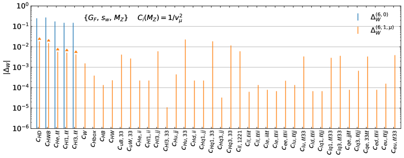
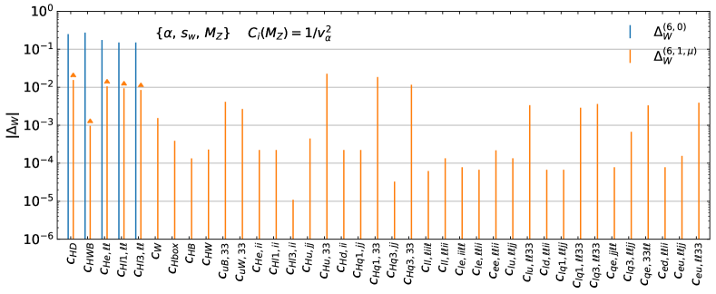
Figure 1: SMEFT corrections to the $W$ boson mass in the $v_{\mu}^{\rm eff}$ (top) and $v_{\alpha}^{\rm eff}$ (bottom) schemes, with $\Delta s_{w}$ determined from $Z\to ee$ decay, so that $\ell=1$. The Wilson coefficients are evaluated at $C_{i}=1/v_{\sigma}^{2}$. The flavour indices $i$ and $j$ run over values $j\in 1,2$, and $i\in 1,2,3$.

		$C_{HWB}$	$C_{HD}$	$C_{\begin{subarray}{c}He\\ 11\end{subarray}}$	$C^{(3)}_{\begin{subarray}{c}Hl\\ 11\end{subarray}}$
LO	$v_{\sigma}^{\rm eff}$	$-0.275_{-0.009}^{+0.009}$	$-0.250_{-0.017}^{+0.017}$	$-0.175_{-0.004}^{+0.004}$	$-0.151_{-0.003}^{+0.003}$
NLO	$v_{\mu}^{\rm eff}$	$-0.290_{-0.000}^{+0.001}$	$-0.269_{-0.000}^{+0.003}$	$-0.180_{-0.000}^{+0.000}$	$-0.161_{-0.000}^{+0.000}$
	$v_{\alpha}^{\rm eff}$	$-0.276_{-0.000}^{+0.000}$	$-0.266_{-0.000}^{+0.002}$	$-0.185_{-0.000}^{+0.000}$	$-0.159_{-0.000}^{+0.000}$
$\text{NLO}_{t}$	$v_{\mu}^{\rm eff}$	$-0.280_{-0.002}^{+0.003}$	$-0.261_{-0.003}^{+0.006}$	$-0.178_{-0.000}^{+0.000}$	$-0.158_{-0.001}^{+0.001}$
	$v_{\alpha}^{\rm eff}$	$-0.272_{-0.002}^{+0.002}$	$-0.261_{-0.003}^{+0.006}$	$-0.183_{-0.000}^{+0.000}$	$-0.158_{-0.001}^{+0.001}$
		$C^{(1)}_{\begin{subarray}{c}Hl\\ 11\end{subarray}}$	$C_{\begin{subarray}{c}Hu\\ 33\end{subarray}}$	$C^{(1)}_{\begin{subarray}{c}Hq\\ 33\end{subarray}}$	$C^{(3)}_{\begin{subarray}{c}Hq\\ 33\end{subarray}}$
LO	$v_{\sigma}^{\rm eff}$	$-0.151_{-0.004}^{+0.004}$	$0.000_{-0.026}^{+0.026}$	$0.000_{-0.026}^{+0.026}$	$0.000_{-0.001}^{+0.001}$
NLO	$v_{\mu}^{\rm eff}$	$-0.156_{-0.000}^{+0.000}$	$0.023_{-0.007}^{+0.000}$	$-0.019_{-0.000}^{+0.006}$	$0.012_{-0.002}^{+0.000}$
	$v_{\alpha}^{\rm eff}$	$-0.160_{-0.000}^{+0.000}$	$0.023_{-0.006}^{+0.000}$	$-0.019_{-0.000}^{+0.006}$	$0.012_{-0.002}^{+0.000}$
$\text{NLO}_{t}$	$v_{\mu}^{\rm eff}$	$-0.154_{-0.000}^{+0.000}$	$0.024_{-0.005}^{+0.000}$	$-0.024_{-0.000}^{+0.005}$	$0.009_{-0.002}^{+0.000}$
	$v_{\alpha}^{\rm eff}$	$-0.158_{-0.000}^{+0.000}$	$0.024_{-0.005}^{+0.000}$	$-0.024_{-0.000}^{+0.005}$	$0.009_{-0.002}^{+0.000}$

Table 4: The numerical prefactors of the Wilson coefficients in the $v_{\mu}^{\rm eff}$ and $v_{\alpha}^{\rm eff}$ schemes contributing to $\Delta_{W}$ for the LO, NLO and NLO_t (large-$m_{t}$ limit) perturbative approximations. The SM tree-level approximation along with $v_{\mu}^{2}$ has been factored out. The results have been evaluated at $\mu$ = $M_{Z}$ and varied up and down by a factor of 2 to give the uncertainties. Only Wilson coefficients whose numerical prefactor is greater than 1% at NLO have been included.

Results for derived parameters in SMEFT depend on a number of Wilson coefficients and are thus quite lengthy. For brevity, we focus the discussion on $M_{W}$ in the $v_{\sigma}^{\rm eff}$ schemes, leaving a comparison of observables across schemes to the heavy-boson decay rates presented in section 3.2.

We show in figure 1 the LO and NLO SMEFT corrections to $M_{W}$ in the $v_{\sigma}^{\rm eff}$ schemes. The numerical contribution from each Wilson coefficient at the scale $\mu=M_{Z}$ is obtained by making the choice $C_{i}(M_{Z})=1/v_{\sigma}^{2}$, and the results are given in units of $M_{W}^{\rm eff}$; in other words, we are quoting results for the expansion coefficients of $\Delta_{W}$ as defined in eq. (40). A remarkable feature is the large number of Wilson coefficients contributing to $M_{W}$ for arbitrary flavour structure; the exact number of coefficients at LO (NLO) is 5 (63) in both schemes. Out of these, 34 Wilson coefficients appearing at NLO correspond to different flavour structures of ten four-fermion operators. The number of Wilson coefficients is reduced when we employ additional flavour assumptions. For concreteness, we consider the scenario of minimal flavour violation (MFV) where the top Yukawa DAmbrosio:2002vsn is the only source of the breaking of the $U(3)^{5}$ symmetry in SMEFT, see appendix B. Under the MFV assumption, 34 Wilson coefficients contribute to $\Delta_{W}$ at NLO, 16 of which correspond to different flavour structures of the ten four-fermion operators.

It is clear from figure 1 that many of the NLO SMEFT corrections to $M_{W}$ are numerically small when all Wilson coefficients are set to a common value. In table 4, we give numerical results at LO and NLO (defined as the sum of LO plus the NLO correction) for those SMEFT operators whose NLO contribution is larger than $1\%$ for the default choice $C_{i}(M_{Z})=1/v_{\sigma}^{2}$. All of these coefficients receive NLO corrections from top loops, and to show their significance we give results where only the large-$m_{t}$ limit of these corrections is used (NLO_t in the table). In each case, we include scale uncertainties obtained by evaluating the prediction for the three scale choices $\mu\in[M_{Z},\,2M_{Z},\,M_{Z}/2]$, using eq. (39) to express the results in terms of $C_{i}(M_{Z})$. In most cases there is a good convergence between LO and NLO when scale uncertainties are included. The large-$m_{t}$ limit results are generally an improvement for central values, but come with small scale uncertainties which do not always overlap with the complete NLO result.

3.2 Heavy boson decays at NLO

In this section we analyse $W\to\tau\nu$ and $Z\to\tau\tau$ decays, focussing on a comparison between input schemes. We define SMEFT expansion coefficients for the decay $X\to f_{1}f_{2}$ in input scheme $s$ as

$$\Gamma(X\to f_{1}f_{2}) =\Gamma^{s(4,0)}_{Xf_{1}f_{2}}+\Gamma^{s(6,0)}_{Xf_{1}f_{2}}+\Gamma^{s(4,1)}_{Xf_{1}f_{2}}+\Gamma^{s(6,1)}_{Xf_{1}f_{2}}\,.$$ (45)

Moreover, we write LO and NLO results as

$$\Gamma^{s}_{Xf_{1}f_{2},\text{LO}} \equiv\Gamma^{s(4,0)}_{Xf_{1}f_{2}}+\Gamma^{s(6,0)}_{Xf_{1}f_{2}}\,,$$

$$\Gamma^{s}_{Xf_{1}f_{2},\text{NLO}} \equiv\Gamma^{s}_{Xf_{1}f_{2}s,\text{LO}}+\Gamma^{s(4,1)}_{Xf_{1}f_{2}}+\Gamma^{s(6,1)}_{Xf_{1}f_{2}}\,.$$ (46)

The LO results for $s\in\{v_{\mu}^{\rm eff},v_{\alpha}^{\rm eff}\}$ are given by

$$\Gamma^{s}_{W\tau\nu,\text{LO}} =\frac{M_{W}^{\rm eff}}{12\pi}\left\{\left(\frac{M_{W}^{\rm eff}}{v_{\sigma}}\right)^{2}+(M_{W}^{\rm eff})^{2}\left[2C_{\begin{subarray}{c}Hl\\ 33\end{subarray}}^{(3)}+3\Delta_{W}^{(6,0)}-\Delta v_{\sigma}^{(6,0)}\right]\right\}\,,$$

$$\Gamma^{s}_{Z\tau\tau,\text{LO}} =\frac{M_{Z}}{24\pi}\bigg{\{}\frac{M_{Z}^{2}}{v_{\sigma}^{2}}\left(1-\frac{v_{\sigma}^{2}}{2}C_{HD}\right)g^{(4,0)}+M_{Z}^{2}\Big{[}\left(2\left(g_{R}^{\ell(6,0)}-g_{L}^{\ell(6,0)}\right)-\Delta v_{\sigma}^{(6,0)}\right)g^{(4,0)}$$

$$+2c_{2w}\left(g_{L}^{\tau(6,0)}-g_{L}^{\ell(6,0)}\right)+4s_{w}^{2}\left(g_{R}^{\tau(6,0)}-g_{R}^{\ell(6,0)}\right)\Big{]}\bigg{\}}\,,$$ (47)

where $\ell\equiv\ell^{i}$ is the charged lepton species used in the definition of $\Delta s_{w}$ and

$$g^{(4,0)} =1-4s_{w}^{2}+8s_{w}^{4}\,.$$ (48)

To derive the result for $W$ decay we have written $W$-mass dependence arising both through two-body phase-space and in the matrix element squared in terms of $M_{W}^{\rm eff}$. Note that in $Z$ decay the flavour-independent coupling $G^{(6,0)}$ given in eq. (2.1) has dropped out of the decay rate due to a cancellation against $\Delta s_{w}^{(6,0)}$. Further simplifications occur only if $\ell=\tau$ or a flavour symmetry such as MFV is imposed, in which case the contribution in the final line vanishes.

		$\Gamma^{s}_{W\ell\nu}$/ $\Gamma_{W\ell\nu}^{\text{exp}}-1$	$\Gamma^{s}_{Z\ell\ell}$/$\Gamma_{Z\ell\ell}^{\text{exp}}-1$
$v_{\mu}^{\rm eff}$	LO	$-1.30\%$	$-0.70\%$
	NLO	$0.16\%$	$0.12\%$
$v_{\alpha}^{\rm eff}$	LO	$-1.51\%$	$-0.91\%$
	NLO	$-0.06\%$	$-0.11\%$
$\alpha_{\mu}$	LO	$0.37\%$	$-0.08\%$
	NLO	$0.03\%$	$-0.07\%$
$\alpha$	LO	$2.87\%$	$2.41\%$
	NLO	$-0.66\%$	$-0.74\%$
LEP	LO	$-1.17\%$	$-0.66\%$
	NLO	$0.31\%$	$0.16\%$

Table 5: Deviations of the SM predictions for $Z\to\ell\ell$ and $W\to\ell\nu$ decay rates in scheme $s$ from the experimental measurements of $\Gamma_{Z\ell\ell}^{\text{exp}}=83.98$ MeV and $\Gamma_{W\ell\nu}^{\text{exp}}=226.4$ MeV ParticleDataGroup:2022pth .

		$C_{HD}$	$C_{HWB}$	$C_{\begin{subarray}{c}He\\ 33\end{subarray}}$	$C_{\begin{subarray}{c}Hu\\ 33\end{subarray}}$	$C^{(3)}_{\begin{subarray}{c}Hq\\ 33\end{subarray}}$
$v_{\mu}^{\rm eff}$	LO	$-0.500_{-0.033}^{+0.033}$	$0.000_{-0.000}^{+0.000}$	$-1.843_{-0.048}^{+0.048}$	$0.000_{-0.052}^{+0.052}$	$0.000_{-0.000}^{+0.000}$
	NLO	$-0.527_{-0.000}^{+0.005}$	$0.004_{-0.000}^{+0.000}$	$-1.905_{-0.000}^{+0.004}$	$0.048_{-0.013}^{+0.000}$	$0.022_{-0.004}^{+0.000}$
$v_{\alpha}^{\rm eff}$	LO	$0.000_{-0.000}^{+0.000}$	$2.370_{-0.081}^{+0.081}$	$-1.843_{-0.050}^{+0.050}$	$0.000_{-0.003}^{+0.003}$	$0.000_{-0.005}^{+0.005}$
	NLO	$-0.001_{-0.000}^{+0.000}$	$2.439_{-0.006}^{+0.000}$	$-1.903_{-0.000}^{+0.004}$	$0.005_{-0.001}^{+0.000}$	$0.002_{-0.000}^{+0.000}$
$\alpha_{\mu}$	LO	$-0.169_{-0.011}^{+0.011}$	$0.355_{-0.012}^{+0.012}$	$-1.764_{-0.046}^{+0.046}$	$0.000_{-0.018}^{+0.018}$	$0.000_{-0.001}^{+0.001}$
	NLO	$-0.289_{-0.007}^{+0.009}$	$0.258_{-0.004}^{+0.003}$	$-1.897_{-0.002}^{+0.006}$	$0.018_{-0.016}^{+0.011}$	$0.006_{-0.002}^{+0.000}$
$\alpha$	LO	$1.573_{-0.108}^{+0.108}$	$4.088_{-0.143}^{+0.143}$	$-1.764_{-0.050}^{+0.050}$	$0.000_{-0.162}^{+0.162}$	$0.000_{-0.008}^{+0.008}$
	NLO	$1.408_{-0.019}^{+0.002}$	$3.869_{-0.013}^{+0.002}$	$-1.898_{-0.002}^{+0.006}$	$-0.142_{-0.000}^{+0.030}$	$-0.073_{-0.000}^{+0.014}$
LEP	LO	$-0.600_{-0.040}^{+0.040}$	$-0.474_{-0.016}^{+0.016}$	$-1.837_{-0.048}^{+0.048}$	$0.000_{-0.062}^{+0.062}$	$0.000_{-0.001}^{+0.001}$
	NLO	$-0.631_{-0.000}^{+0.005}$	$-0.475_{-0.000}^{+0.001}$	$-1.899_{-0.000}^{+0.004}$	$0.057_{-0.015}^{+0.000}$	$0.025_{-0.005}^{+0.000}$

Table 6: Selected SMEFT contributions to the $Z\to\tau\tau$ decay rate including scale variation in the five schemes.

The LO and NLO results for $W$ and $Z$ decay in the SM are shown in table 5, where we have normalised the results to the experimentally measured values. The NLO corrections in the SM bring results from all five schemes into close numerical agreement. These corrections are at the $1.5\%$ level for $W$ decay in the $v_{\sigma}^{\rm eff}$ and LEP schemes, where $M_{W}$ is not an input and hence factors of $3\Delta_{W}^{s(4,1)}/v_{\sigma}^{2}$ arise compared to the $\alpha_{\mu}$ scheme. Corrections of around $-3\%$ arise in the $\alpha$ scheme, which are mainly due to the top-loop corrections to $s_{w}$ shown in eq. (42). As explained in section 3.1, the close agreement between decay rates at NLO different schemes is a consequence of that for the derived parameters in table 3.

The situation in SMEFT is different, because in that case the relations between input parameters in different schemes depend on the Wilson coefficients and there can be non-trivial interplay with other, process-dependent contributions. Therefore, in general, the numerical prefactor multiplying a particular Wilson coefficient can be very different across schemes. This point is seen in table 6, where the LO and NLO contributions for an illustrative sample of Wilson coefficients are shown for the decay $Z\to\tau\tau$, using $\ell^{i}=e$ to determine the $\Delta s_{w}$ counterterm in the $v_{\sigma}^{\rm eff}$ schemes. The results include perturbative uncertainties obtained by varying the default scale choice $\mu_{\rm def}=M_{Z}$ up and down by a factor of two. We note the following features:

• The contributions from the coefficients $C_{HD}$ and $C_{HWB}$ have rather different prefactors in each scheme, and convergence between LO and NLO also differs markedly from case to case – especially in the $\alpha_{\mu}$ scheme the NLO corrections are large and well outside the LO scale uncertainties.

• By contrast, at LO the coefficient $C_{\begin{subarray}{c}He\\ 33\end{subarray}}$ appears only in the $Z\to\tau\tau$ matrix element. The dominant NLO corrections arise from SM counterterms on this LO vertex, and tend to push the NLO results in different schemes to similar values. The NLO corrections in the $\alpha$ and $\alpha_{\mu}$ schemes are outside the LO scale uncertainties.

• The coefficients $C_{\begin{subarray}{c}Hu\\ 33\end{subarray}}$ and $C^{(3)}_{\begin{subarray}{c}Hq\\ 33\end{subarray}}$ first appear at NLO for fixed $\mu$. The contribution of the former is well estimated by LO scale uncertainties through the running of $C_{HD}$ (driven by the top-loop contribution shown in eq. (A.1)), while that of the latter is unrelated to RG running and requires a genuine NLO calculation.

Regarding the first two points, NLO corrections in the $v_{\sigma}^{\rm eff}$ schemes tend to be milder than in the $\alpha$ or $\alpha_{\mu}$ schemes because in the latter case $\Delta s_{w}$ gets scale-independent corrections of the type shown in eq. (42). In that case including universal corrections from the large-$m_{t}$ limit using the procedure outlined in Biekotter:2023xle can improve convergence between orders. The specific pattern of contributions described above is specific to $Z$ decay, but the important point that the size of SMEFT contributions related to a particular Wilson coefficient is highly scheme specific is general.

		$\Gamma_{W\tau\nu}$		$\Gamma_{Z\tau\tau}$ ($\Gamma_{Zee}$)		Total # unique WC
		gen	MFV	gen	MFV	gen	MFV
$v_{\mu}^{\rm eff}$	LO	8	6	9 (6)	4	10	6
	NLO	69	34	93 (63)	33	93	34
$v_{\alpha}^{\rm eff}$	LO	6	5	7 (4)	4	8	5
	NLO	68	34	92 (63)	34	92	34
$\alpha_{\mu}$	LO	4	1	8 (7)	6	8	6
	NLO	25	14	67 (64)	34	67	34
$\alpha$	LO	3	3	5 (5)	5	5	5
	NLO	35	22	63 (63)	34	63	34
LEP	LO	6	4	8 (7)	6	8	6
	NLO	39	22	67 (64)	34	67	34

Table 7: Number of Wilson coefficients appearing in heavy boson decay rates under general flavour assumptions and MFV. Note that assuming MFV the number of operators appearing in $\Gamma_{Z\tau\tau}$ and $\Gamma_{Zee}$ is the same and hence only one value is given.

The discussion so far highlights the non-trivial pattern of perturbative convergence across schemes. It is also interesting to study the number of Wilson coefficients characteristic of each scheme. In table 7, we show the total number of Wilson coefficients contributing to $W$ and $Z$ decay at LO and NLO in the five input schemes for different flavour assumptions. For both decays, significantly more coefficients are involved in the $v_{\sigma}^{\rm eff}$ schemes than in the others, when no flavour restrictions are made; this is because the counterterm for $s_{w}$ is determined from $Z\to ee$ decay amplitudes, and involves a number of flavour specific left and right-handed fermion gauge couplings in addition to four-fermion operators, which would not otherwise appear in $Z\to\tau\tau$ decay. Indeed, if we consider the decay $Z\to ee$ instead, the number of Wilson coefficients appearing throughout all five schemes is far more similar. The same statement applies if MFV is used – in fact, the number of Wilson coefficients entering the combination of the two decays is the same.

In a full analysis of electroweak precision observables including gauge-boson decays to quarks and $Z$ decay to neutrinos, the total number of Wilson coefficients appearing is further increased through contributions from four-quark operators. For MFV the total number of operators appearing grows from 34 in the leptonic $Z$ and $W$ decays considered here to 56 in the full set of electroweak precision observables Bellafronte:2023amz .

4 Conclusions

We have implemented to NLO in SMEFT two EW input schemes involving $\sin\theta_{\text{eff}}^{\ell}$ as an input parameter. These “$v_{\sigma}^{\rm eff}$ schemes” share as common inputs $\sin\theta_{\text{eff}}^{\ell}$ and $M_{Z}$, but differ through the use of the fine structure constant $\alpha$ ($v_{\alpha}^{\rm eff}$ scheme) or the Fermi constant $G_{F}$ ($v_{\mu}^{\rm eff}$ scheme) as the third independent input parameter. Details of the renormalisation procedure in these schemes were given in section 2, and numerical results for a select set of electroweak precision observables, including comparisons with the other commonly used EW input schemes listed in table 1, were given in section 3. Analytic results in the $v_{\sigma}^{\rm eff}$ schemes which form that basis of that numerical analysis are given in electronic form in the arXiv submission of this paper.

An attractive feature of the $v_{\sigma}^{\rm eff}$ schemes in SMEFT is that sizeable corrections to the sine of the Weinberg angle related to top-quark loops appearing in other schemes are absorbed into the definition of the parameter $\sin\theta_{\text{eff}}^{\ell}$. On the other hand, the renormalisation conditions for $\sin\theta_{\text{eff}}^{\ell}$ are implemented at the level of form factors for two-body $Z\to\ell\ell$ decay, and are thus subject to a large number of flavour-specific $Z$-fermion SMEFT couplings, including four-fermion operators. For instance, the SMEFT expansion for $M_{W}$ in these schemes receives contributions from five Wilson coefficients at LO, but 63 already at NLO, and as shown in table 7 even a simple process such as $Z\to\tau\tau$ is subject to roughly 90 coefficients at NLO. Flavour assumptions on the SMEFT Wilson coefficients imposed by symmetries such as MFV may therefore be an essential ingredient to practical implementations of this scheme in global fits to data.

Regarding such fits, observables in each input scheme are subject to a different pattern of higher-order corrections in both loops and operator dimensions. Therefore, performing fits in multiple EW input schemes can provide an important estimate on the significance of such missing corrections, and is a valuable consistency check on the results in any one scheme. The results of this paper provide an important new component for such analyses.

Appendix A Expansion coefficients and large-$m_{t}$ limit of $\Delta_{W}$ and $\Delta r^{\rm eff}$

In this section we derive the SMEFT expansions of $\Delta_{W}$ and $\Delta r^{\rm eff}$, which are used to predict $M_{W}$, $G_{F}$, and $\alpha$ in the $v_{\sigma}^{\rm eff}$ schemes. We also give explicit results in the large-$m_{t}$ limit.

A.1 SMEFT expansion of $M_{W}$

A simple way to derive the quantity $\Delta_{W}$ defined in eq. (40) is to use the bare mass $M_{W,0}$ as an intermediary:

$$M_{W,0}=M_{W}^{\rm eff}\left(1+\Delta M_{W}^{\rm eff}\right)=M_{W}\left(1+\Delta M_{W}\right)\,.$$ (49)

After expressing the expansion coefficients of the on-shell counterterm $\Delta M_{W}$ in terms of $M_{W}^{\rm eff}$ following the notation of eq. (2.1), one finds

$$\Delta_{W}^{(6,0)} =\Delta M_{W}^{{\rm eff}(6,0)}\,,$$

$$\Delta_{W}^{(4,1)} =\Delta M_{W}^{{\rm eff}(4,1)}-\Delta M_{W}^{(4,1)}\,,$$

$$\Delta_{W}^{(6,1,\sigma)} =\Delta_{W}^{(6,1)}-\Delta_{W}^{(4,1)}\Delta v_{\sigma}^{(6,0)}+\Delta_{W}^{(6,0)}\left(\Delta v_{\sigma}^{(4,1)}-2\Delta M_{W}^{(4,1)}\right)\,,$$ (50)

with

$$\Delta_{W}^{(6,1)} =\Delta M_{W}^{{\rm eff}(6,1)}-\Delta M_{W}^{(6,1)}+\Delta_{W}^{(6,0)}\Delta M_{W}^{(4,1)}\,.$$ (51)

To derive the large-$m_{t}$ limit results we first note the SM results

$$\Delta s_{w,t}^{(4,1)} =\Delta e_{t}^{(4,1)}=0\,,$$

$$\Delta v_{\alpha,t}^{(4,1)} =2\Delta M_{W,t}^{{\rm eff}(4,1)}=2\Delta M_{Z,t}^{(4,1)}\,,$$

$$\Delta v_{\mu,t}^{(4,1)} =2\Delta M_{w,t}^{(4,1)}\,.$$ (52)

One then has for the SM correction to $\Delta_{W}$ in this limit

$$\Delta_{W,t}^{(4,1)} =\Delta M_{Z,t}^{(4,1)}-\Delta M_{W,t}^{(4,1)}=\frac{1}{2}\Delta\rho_{t}^{(4,1)}\,.$$ (53)

The result in SMEFT can be written in the form

$$\Delta_{W,t}^{(6,1,\sigma)} =\Delta_{W,t}^{(6,1)}+\Delta_{W,t}^{(4,1)}\left(2\Delta_{W}^{(6,0)}\delta_{\sigma\alpha}-\Delta v_{\sigma}^{(6,0)}\right)\,,$$ (54)

where $\delta_{\sigma\alpha}$ is the Kronecker delta. An explicit calculation shows that

$$\Delta_{W,t}^{(6,1)} =2\Delta_{W,t}^{(4,1)}\left[C^{(3)}_{\begin{subarray}{c}Hq\\ 33\end{subarray}}-\frac{\sqrt{2}M_{W}^{\rm eff}}{m_{t}}C_{\begin{subarray}{c}uW\\ 33\end{subarray}}-\frac{1}{2}\Delta_{W}^{(6,0)}\right]-v_{\sigma}^{2}\dot{\Delta}_{W,t}^{(6,0)}\ln\frac{\mu}{m_{t}}\,,$$ (55)

where the logarithmic dependence is governed by

$$\dot{\Delta}_{W,t}^{(6,0)} =-\frac{1}{4}\dot{C}_{HD,t}-\frac{s_{w}}{2c_{w}}\dot{C}_{HWB,t}+\frac{s_{w}^{2}}{2c_{w}^{2}}\dot{g}_{L,t}^{\ell(6,0)}+\frac{c_{2w}}{4c_{w}^{2}}\dot{g}_{R,t}^{\ell(6,0)}\,,$$ (56)

with

$$v_{\sigma}^{2}\dot{C}_{HD,t} =8\Delta\rho_{t}^{(4,1)}\left[C_{HD}+2C_{\begin{subarray}{c}Hq\\ 33\end{subarray}}^{(1)}-2C_{\begin{subarray}{c}Hu\\ 33\end{subarray}}\right]\,,$$

$$v_{\sigma}^{2}\dot{C}_{HWB,t} =4\Delta\rho_{t}^{(4,1)}\left[C_{HWB}-\sqrt{2}\frac{M_{Z}}{m_{t}}\left(c_{w}C_{\begin{subarray}{c}uB\\ 33\end{subarray}}+\frac{5}{3}s_{w}C_{\begin{subarray}{c}uW\\ 33\end{subarray}}\right)\right]\,,$$

$$v_{\sigma}^{2}\dot{g}_{L,t}^{\ell(6,0)} =4\Delta\rho_{t}^{(4,1)}\left[g_{L}^{\ell(6,0)}-C^{(1)}_{\begin{subarray}{c}lq\\ ii33\end{subarray}}+C^{(3)}_{\begin{subarray}{c}lq\\ ii33\end{subarray}}+C_{\begin{subarray}{c}lu\\ 33ii\end{subarray}}\right]\,,$$

$$v_{\sigma}^{2}\dot{g}_{R,t}^{\ell(6,0)} =4\Delta\rho_{t}^{(4,1)}\left[g_{R}^{\ell(6,0)}+C_{\begin{subarray}{c}eu\\ ii33\end{subarray}}-C_{\begin{subarray}{c}qe\\ 33ii\end{subarray}}\right]\,.\$$ (57)

A.2 SMEFT expansions of $G_{F}$ and $\alpha$

The expansion coefficients for $\Delta r^{\rm eff}$ defined in eq. (41) are calculated similarly to those for $M_{W}$, except this time using $v_{T,0}$ as an intermediary. In particular, by equating eq. (7) with eq. (8) one finds

$$\Delta r^{{\rm eff}(6,0)} =\Delta v_{\mu}^{(6,0)}-\Delta v_{\alpha}^{(6,0)}\,,$$

$$\Delta r^{{\rm eff}(4,1)} =\Delta v_{\mu}^{(4,1)}-\Delta v_{\alpha}^{(4,1)}\,,$$

$$\Delta r^{{\rm eff}(6,1)} =\Delta v_{\mu}^{(6,1)}-\Delta v_{\alpha}^{(6,1)}+2\Delta v_{\mu}^{(4,1)}\Delta r^{{\rm eff}(6,0)}\,.$$ (58)

Following the discussion of universal corrections in Biekotter:2023xle , we write the results in the large-$m_{t}$ limit in the form

$$\Delta r_{t}^{{\rm eff}(i,j)}=K_{\alpha}^{(i,j)}-K_{\mu}^{(i,j)}\,.$$ (59)

Results for the $K_{\mu}$ can be read off from Biekotter:2023xle (after adapting to our notation), while the results for $K_{\alpha}$ are new. The one-loop result in the SM is

$$K_{\sigma}^{(4,1)} =-\Delta\rho_{t}^{(4,1)}\delta_{\alpha\sigma}\,.$$ (60)

The SMEFT answer takes the form

$$K_{\sigma}^{(6,0)} =-\Delta v_{\sigma}^{(6,0)}\,,$$

$$K_{\sigma}^{(6,1)} =-\frac{1}{2}v_{\sigma}^{2}\dot{K}_{\sigma,t}^{(6,0)}\ln\frac{\mu^{2}}{m_{t}^{2}}+k_{\sigma}^{(6,1)}\,.$$ (61)

One has, for the non-logarithmic pieces

$$k_{\mu}^{(6,1)} =\Delta\rho_{t}^{(4,1)}\sum_{j=1,2}\bigg{[}C_{\begin{subarray}{c}Hl\\ jj\end{subarray}}^{(3)}-C^{(3)}_{\begin{subarray}{c}lq\\ jj33\end{subarray}}\bigg{]}\,,$$

$$k_{\alpha}^{(6,1)} =2K_{\alpha}^{(4,1)}\left(K_{\alpha}^{(6,0)}+C_{\begin{subarray}{c}Hq\\ 33\end{subarray}}^{(3)}\right)\,,$$ (62)

whereas the dependence on the renormalisation scale $\mu$ is governed by

$$v_{\sigma}^{2}\dot{K}_{\mu,t}^{(6,0)} =-4\Delta\rho_{t}^{(4,1)}\sum_{j=1,2}\bigg{[}C_{\begin{subarray}{c}Hl\\ jj\end{subarray}}^{(3)}-C^{(3)}_{\begin{subarray}{c}lq\\ jj33\end{subarray}}\bigg{]}\,,$$

$$v_{\sigma}^{2}\dot{K}_{\alpha,t}^{(6,0)} =\frac{1}{2}\dot{C}_{HD,t}+\frac{1}{c_{w}s_{w}}\dot{C}_{HWB,t}+\frac{c_{2w}}{c_{w}^{2}}\left(\dot{g}_{L,t}^{\ell(6,0)}+\frac{c_{2w}}{2s_{w}^{2}}\dot{g}_{R,t}^{\ell(6,0)}\right)\,.$$ (63)

All components needed to evaluate the latter result were given in eq. (A.1).

Appendix B Minimal flavour violation

The calculations in this work have been performed with no assumptions on the flavour structure of the SMEFT operators. To reduce the number of free parameters, we can make the assumption of minimal flavour violation (MFV). In this appendix, we give details on this flavour scenario.

In the SM, the $U(3)^{5}$ symmetry for the SM fermions

$$U(3)^{5}\equiv U(3)_{q}\times U(3)_{l}\times U(3)_{u}\times U(3)_{d}\times U(3)_{e}\,,$$ (64)

is broken only by the Yukawa couplings Gerard:1982mm ; Chivukula:1987py . The MFV scenario extends this requirement to SMEFT DAmbrosio:2002vsn . Since we consider all fermions except the top quark to be massless, we only thus only allow the breaking of the $U(3)^{5}$ symmetry by the top Yukawa coupling $Y_{t}$. In the MFV case, we thus distinguish Wilson coefficients involving the top quark from those involving first and second-generation up-type quarks.

We change from the flavour-general scenario to MFV by making a set of replacements on the Wilson coefficients, see e.g. Bellafronte:2023amz . For operators with two flavour indices involving leptons or down-type quarks, we can suppress the flavour indices

$$C_{\begin{subarray}{c}x\\ ii\end{subarray}}\to C_{x},\quad\text{for }C_{x}\in C_{He},\,C_{Hl}^{(1)},\,C_{Hl}^{(3)},\,C_{Hd}\,.$$ (65)

For the Wilson coefficients with two flavour indices involving up-type quark fields, we explicitly distinguish top-quark couplings

$$C_{\begin{subarray}{c}x\\ jj\end{subarray}}\to C_{x}\text{ for }j\in 1,\,2\,,\quad C_{\begin{subarray}{c}Hu\\ 33\end{subarray}}\to C_{Ht},\quad C^{(1)}_{\begin{subarray}{c}Hq\\ 33\end{subarray}}\to C^{(1)}_{HQ},\quad C^{(3)}_{\begin{subarray}{c}Hq\\ 33\end{subarray}}\to C^{(3)}_{HQ}\,.$$ (66)

For $C_{uB}$ and $C_{uW}$ only Wilson coefficients with third-family indices contribute in the first place so no replacement is necessary.

For four-fermion operators with two different fermion bilinears as well as $C_{ee}$, which is simplified by a Fierz identity, there is a single coefficient contributing under the MFV assumption when no up-type quarks are involved

$$C_{\begin{subarray}{c}x\\ iijj\end{subarray}}\to C_{x}\quad\text{for }C_{x}\in C_{ee},\,C_{le},\,C_{ld},\,C_{ed}\,.$$ (67)

In Wilson coefficients involving up-type quark fields we distinguish the third generation

$$C_{\begin{subarray}{c}x\\ iijj\end{subarray}}\to C_{x}\text{ for }j\in 1,\,2,\quad C_{\begin{subarray}{c}lq\\ ii33\end{subarray}}^{(1)} \to C^{(1)}_{lQ},\quad C_{\begin{subarray}{c}lq\\ ii33\end{subarray}}^{(3)}\to C^{(3)}_{lQ},\quad C_{\begin{subarray}{c}lu\\ ii33\end{subarray}}\to C_{lt},\quad$$

$$C_{\begin{subarray}{c}qe\\ jjii\end{subarray}}\to C_{qe}\text{ for }j\in 1,\,2,\quad C_{\begin{subarray}{c}qe\\ 33ii\end{subarray}} \to C_{Qe}\quad\,.$$ (68)

For $C_{ll}$, which involves two fermion currents of the same species and chirality, there are two $U(3)^{5}$ symmetric combinations, which we distinguish with a prime

$$C_{\begin{subarray}{c}ll\\ iijj\end{subarray}}\to C_{ll},\quad C_{\begin{subarray}{c}ll\\ ijji\end{subarray}}\to C_{ll}^{\prime},\quad C_{\begin{subarray}{c}ll\\ iiii\end{subarray}}\to C_{ll}+C_{ll}^{\prime}\,.$$ (69)

$1:X^{3}$
$Q_{G}$	$f^{ABC}G_{\mu}^{A\nu}G_{\nu}^{B\rho}G_{\rho}^{C\mu}$
$Q_{\widetilde{G}}$	$f^{ABC}\widetilde{G}_{\mu}^{A\nu}G_{\nu}^{B\rho}G_{\rho}^{C\mu}$
$Q_{W}$	$\epsilon^{IJK}W_{\mu}^{I\nu}W_{\nu}^{J\rho}W_{\rho}^{K\mu}$
$Q_{\widetilde{W}}$	$\epsilon^{IJK}\widetilde{W}_{\mu}^{I\nu}W_{\nu}^{J\rho}W_{\rho}^{K\mu}$

$2:H^{6}$
$Q_{H}$	$(H^{\dagger}H)^{3}$

$3:H^{4}D^{2}$
$Q_{H\Box}$	$(H^{\dagger}H)\Box(H^{\dagger}H)$
$Q_{HD}$	$\ \left(H^{\dagger}D_{\mu}H\right)^{*}\left(H^{\dagger}D_{\mu}H\right)$

$5:\psi^{2}H^{3}+\hbox{h.c.}$
$Q_{eH}$	$(H^{\dagger}H)(\bar{l}_{p}e_{r}H)$
$Q_{uH}$	$(H^{\dagger}H)(\bar{q}_{p}u_{r}\widetilde{H})$
$Q_{dH}$	$(H^{\dagger}H)(\bar{q}_{p}d_{r}H)$

$4:X^{2}H^{2}$
$Q_{HG}$	$H^{\dagger}H\,G^{A}_{\mu\nu}G^{A\mu\nu}$
$Q_{H\widetilde{G}}$	$H^{\dagger}H\,\widetilde{G}^{A}_{\mu\nu}G^{A\mu\nu}$
$Q_{HW}$	$H^{\dagger}H\,W^{I}_{\mu\nu}W^{I\mu\nu}$
$Q_{H\widetilde{W}}$	$H^{\dagger}H\,\widetilde{W}^{I}_{\mu\nu}W^{I\mu\nu}$
$Q_{HB}$	$H^{\dagger}H\,B_{\mu\nu}B^{\mu\nu}$
$Q_{H\widetilde{B}}$	$H^{\dagger}H\,\widetilde{B}_{\mu\nu}B^{\mu\nu}$
$Q_{HWB}$	$H^{\dagger}\sigma^{I}H\,W^{I}_{\mu\nu}B^{\mu\nu}$
$Q_{H\widetilde{W}B}$	$H^{\dagger}\sigma^{I}H\,\widetilde{W}^{I}_{\mu\nu}B^{\mu\nu}$

$6:\psi^{2}XH+\hbox{h.c.}$
$Q_{eW}$	$(\bar{l}_{p}\sigma^{\mu\nu}e_{r})\sigma^{I}HW_{\mu\nu}^{I}$
$Q_{eB}$	$(\bar{l}_{p}\sigma^{\mu\nu}e_{r})HB_{\mu\nu}$
$Q_{uG}$	$(\bar{q}_{p}\sigma^{\mu\nu}T^{A}u_{r})\widetilde{H}\,G_{\mu\nu}^{A}$
$Q_{uW}$	$(\bar{q}_{p}\sigma^{\mu\nu}u_{r})\sigma^{I}\widetilde{H}\,W_{\mu\nu}^{I}$
$Q_{uB}$	$(\bar{q}_{p}\sigma^{\mu\nu}u_{r})\widetilde{H}\,B_{\mu\nu}$
$Q_{dG}$	$(\bar{q}_{p}\sigma^{\mu\nu}T^{A}d_{r})H\,G_{\mu\nu}^{A}$
$Q_{dW}$	$(\bar{q}_{p}\sigma^{\mu\nu}d_{r})\sigma^{I}H\,W_{\mu\nu}^{I}$
$Q_{dB}$	$(\bar{q}_{p}\sigma^{\mu\nu}d_{r})H\,B_{\mu\nu}$

$7:\psi^{2}H^{2}D$
$Q_{Hl}^{(1)}$	$(H^{\dagger}i\overleftrightarrow{D}_{\mu}H)(\bar{l}_{p}\gamma^{\mu}l_{r})$
$Q_{Hl}^{(3)}$	$(H^{\dagger}i\overleftrightarrow{D}^{I}_{\mu}H)(\bar{l}_{p}\sigma^{I}\gamma^{\mu}l_{r})$
$Q_{He}$	$(H^{\dagger}i\overleftrightarrow{D}_{\mu}H)(\bar{e}_{p}\gamma^{\mu}e_{r})$
$Q_{Hq}^{(1)}$	$(H^{\dagger}i\overleftrightarrow{D}_{\mu}H)(\bar{q}_{p}\gamma^{\mu}q_{r})$
$Q_{Hq}^{(3)}$	$(H^{\dagger}i\overleftrightarrow{D}^{I}_{\mu}H)(\bar{q}_{p}\sigma^{I}\gamma^{\mu}q_{r})$
$Q_{Hu}$	$(H^{\dagger}i\overleftrightarrow{D}_{\mu}H)(\bar{u}_{p}\gamma^{\mu}u_{r})$
$Q_{Hd}$	$(H^{\dagger}i\overleftrightarrow{D}_{\mu}H)(\bar{d}_{p}\gamma^{\mu}d_{r})$
$Q_{Hud}$ + h.c.	$i(\widetilde{H}^{\dagger}D_{\mu}H)(\bar{u}_{p}\gamma^{\mu}d_{r})$

$8:(\bar{L}L)(\bar{L}L)$
$Q_{ll}$	$(\bar{l}_{p}\gamma_{\mu}l_{r})(\bar{l}_{s}\gamma^{\mu}l_{t})$
$Q_{qq}^{(1)}$	$(\bar{q}_{p}\gamma_{\mu}q_{r})(\bar{q}_{s}\gamma^{\mu}q_{t})$
$Q_{qq}^{(3)}$	$(\bar{q}_{p}\gamma_{\mu}\sigma^{I}q_{r})(\bar{q}_{s}\gamma^{\mu}\sigma^{I}q_{t})$
$Q_{lq}^{(1)}$	$(\bar{l}_{p}\gamma_{\mu}l_{r})(\bar{q}_{s}\gamma^{\mu}q_{t})$
$Q_{lq}^{(3)}$	$(\bar{l}_{p}\gamma_{\mu}\sigma^{I}l_{r})(\bar{q}_{s}\gamma^{\mu}\sigma^{I}q_{t})$

$8:(\bar{R}R)(\bar{R}R)$
$Q_{ee}$	$(\bar{e}_{p}\gamma_{\mu}e_{r})(\bar{e}_{s}\gamma^{\mu}e_{t})$
$Q_{uu}$	$(\bar{u}_{p}\gamma_{\mu}u_{r})(\bar{u}_{s}\gamma^{\mu}u_{t})$
$Q_{dd}$	$(\bar{d}_{p}\gamma_{\mu}d_{r})(\bar{d}_{s}\gamma^{\mu}d_{t})$
$Q_{eu}$	$(\bar{e}_{p}\gamma_{\mu}e_{r})(\bar{u}_{s}\gamma^{\mu}u_{t})$
$Q_{ed}$	$(\bar{e}_{p}\gamma_{\mu}e_{r})(\bar{d}_{s}\gamma^{\mu}d_{t})$
$Q_{ud}^{(1)}$	$(\bar{u}_{p}\gamma_{\mu}u_{r})(\bar{d}_{s}\gamma^{\mu}d_{t})$
$Q_{ud}^{(8)}$	$(\bar{u}_{p}\gamma_{\mu}T^{A}u_{r})(\bar{d}_{s}\gamma^{\mu}T^{A}d_{t})$

$8:(\bar{L}L)(\bar{R}R)$
$Q_{le}$	$(\bar{l}_{p}\gamma_{\mu}l_{r})(\bar{e}_{s}\gamma^{\mu}e_{t})$
$Q_{lu}$	$(\bar{l}_{p}\gamma_{\mu}l_{r})(\bar{u}_{s}\gamma^{\mu}u_{t})$
$Q_{ld}$	$(\bar{l}_{p}\gamma_{\mu}l_{r})(\bar{d}_{s}\gamma^{\mu}d_{t})$
$Q_{qe}$	$(\bar{q}_{p}\gamma_{\mu}q_{r})(\bar{e}_{s}\gamma^{\mu}e_{t})$
$Q_{qu}^{(1)}$	$(\bar{q}_{p}\gamma_{\mu}q_{r})(\bar{u}_{s}\gamma^{\mu}u_{t})$
$Q_{qu}^{(8)}$	$(\bar{q}_{p}\gamma_{\mu}T^{A}q_{r})(\bar{u}_{s}\gamma^{\mu}T^{A}u_{t})$
$Q_{qd}^{(1)}$	$(\bar{q}_{p}\gamma_{\mu}q_{r})(\bar{d}_{s}\gamma^{\mu}d_{t})$
$Q_{qd}^{(8)}$	$(\bar{q}_{p}\gamma_{\mu}T^{A}q_{r})(\bar{d}_{s}\gamma^{\mu}T^{A}d_{t})$

$8:(\bar{L}R)(\bar{R}L)+\hbox{h.c.}$
$Q_{ledq}$	$(\bar{l}_{p}^{j}e_{r})(\bar{d}_{s}q_{tj})$

$8:(\bar{L}R)(\bar{L}R)+\hbox{h.c.}$
$Q_{quqd}^{(1)}$	$(\bar{q}_{p}^{j}u_{r})\epsilon_{jk}(\bar{q}_{s}^{k}d_{t})$
$Q_{quqd}^{(8)}$	$(\bar{q}_{p}^{j}T^{A}u_{r})\epsilon_{jk}(\bar{q}_{s}^{k}T^{A}d_{t})$
$Q_{lequ}^{(1)}$	$(\bar{l}_{p}^{j}e_{r})\epsilon_{jk}(\bar{q}_{s}^{k}u_{t})$
$Q_{lequ}^{(3)}$	$(\bar{l}_{p}^{j}\sigma_{\mu\nu}e_{r})\epsilon_{jk}(\bar{q}_{s}^{k}\sigma^{\mu\nu}u_{t})$

Table 8: The 59 independent baryon number conserving dimension-six operators built from Standard Model fields, in the notation of Jenkins:2013zja . The subscripts $p,r,s,t$ are flavour indices, and $\sigma^{I}$ are Pauli matrices.

References

• (1) W. Buchmuller and D. Wyler, Effective Lagrangian Analysis of New Interactions and Flavor Conservation, Nucl. Phys. B 268 (1986) 621.
• (2) F. Wilczek, Problem of Strong $P$ and $T$ Invariance in the Presence of Instantons, Phys. Rev. Lett. 40 (1978) 279.
• (3) B. Grzadkowski, M. Iskrzynski, M. Misiak and J. Rosiek, Dimension-Six Terms in the Standard Model Lagrangian, JHEP 10 (2010) 085 [1008.4884].
• (4) C. Degrande, G. Durieux, F. Maltoni, K. Mimasu, E. Vryonidou and C. Zhang, Automated one-loop computations in the standard model effective field theory, Phys. Rev. D 103 (2021) 096024 [2008.11743].
• (5) C. Zhang and F. Maltoni, Top-quark decay into Higgs boson and a light quark at next-to-leading order in QCD, Phys. Rev. D 88 (2013) 054005 [1305.7386].
• (6) A. Crivellin, S. Najjari and J. Rosiek, Lepton Flavor Violation in the Standard Model with general Dimension-Six Operators, JHEP 04 (2014) 167 [1312.0634].
• (7) C. Zhang, Effective field theory approach to top-quark decay at next-to-leading order in QCD, Phys. Rev. D 90 (2014) 014008 [1404.1264].
• (8) G.M. Pruna and A. Signer, The $\mu\to e\gamma$ decay in a systematic effective field theory approach with dimension 6 operators, JHEP 10 (2014) 014 [1408.3565].
• (9) R. Grober, M. Muhlleitner, M. Spira and J. Streicher, NLO QCD Corrections to Higgs Pair Production including Dimension-6 Operators, JHEP 09 (2015) 092 [1504.06577].
• (10) C. Hartmann and M. Trott, On one-loop corrections in the standard model effective field theory; the $\Gamma(h\rightarrow\gamma\,\gamma)$ case, JHEP 07 (2015) 151 [1505.02646].
• (11) M. Ghezzi, R. Gomez-Ambrosio, G. Passarino and S. Uccirati, NLO Higgs effective field theory and $\kappa$-framework, JHEP 07 (2015) 175 [1505.03706].
• (12) C. Hartmann and M. Trott, Higgs Decay to Two Photons at One Loop in the Standard Model Effective Field Theory, Phys. Rev. Lett. 115 (2015) 191801 [1507.03568].
• (13) R. Gauld, B.D. Pecjak and D.J. Scott, One-loop corrections to $h\to b\bar{b}$ and $h\to\tau\bar{\tau}$ decays in the Standard Model Dimension-6 EFT: four-fermion operators and the large-$m_{t}$ limit, JHEP 05 (2016) 080 [1512.02508].
• (14) J. Aebischer, A. Crivellin, M. Fael and C. Greub, Matching of gauge invariant dimension-six operators for $b\to s$ and $b\to c$ transitions, JHEP 05 (2016) 037 [1512.02830].
• (15) C. Zhang, Single Top Production at Next-to-Leading Order in the Standard Model Effective Field Theory, Phys. Rev. Lett. 116 (2016) 162002 [1601.06163].
• (16) O. Bessidskaia Bylund, F. Maltoni, I. Tsinikos, E. Vryonidou and C. Zhang, Probing top quark neutral couplings in the Standard Model Effective Field Theory at NLO in QCD, JHEP 05 (2016) 052 [1601.08193].
• (17) F. Maltoni, E. Vryonidou and C. Zhang, Higgs production in association with a top-antitop pair in the Standard Model Effective Field Theory at NLO in QCD, JHEP 10 (2016) 123 [1607.05330].
• (18) R. Gauld, B.D. Pecjak and D.J. Scott, QCD radiative corrections for $h\to b\bar{b}$ in the Standard Model Dimension-6 EFT, Phys. Rev. D 94 (2016) 074045 [1607.06354].
• (19) C. Degrande, B. Fuks, K. Mawatari, K. Mimasu and V. Sanz, Electroweak Higgs boson production in the standard model effective field theory beyond leading order in QCD, Eur. Phys. J. C 77 (2017) 262 [1609.04833].
• (20) C. Hartmann, W. Shepherd and M. Trott, The $Z$ decay width in the SMEFT: $y_{t}$ and $\lambda$ corrections at one loop, JHEP 03 (2017) 060 [1611.09879].
• (21) M. Grazzini, A. Ilnicka, M. Spira and M. Wiesemann, Modeling BSM effects on the Higgs transverse-momentum spectrum in an EFT approach, JHEP 03 (2017) 115 [1612.00283].
• (22) D. de Florian, I. Fabre and J. Mazzitelli, Higgs boson pair production at NNLO in QCD including dimension 6 operators, JHEP 10 (2017) 215 [1704.05700].
• (23) N. Deutschmann, C. Duhr, F. Maltoni and E. Vryonidou, Gluon-fusion Higgs production in the Standard Model Effective Field Theory, JHEP 12 (2017) 063 [1708.00460].
• (24) J. Baglio, S. Dawson and I.M. Lewis, An NLO QCD effective field theory analysis of $W^{+}W^{-}$ production at the LHC including fermionic operators, Phys. Rev. D 96 (2017) 073003 [1708.03332].
• (25) S. Dawson and P.P. Giardino, Higgs decays to $ZZ$ and $Z\gamma$ in the standard model effective field theory: An NLO analysis, Phys. Rev. D 97 (2018) 093003 [1801.01136].
• (26) C. Degrande, F. Maltoni, K. Mimasu, E. Vryonidou and C. Zhang, Single-top associated production with a $Z$ or $H$ boson at the LHC: the SMEFT interpretation, JHEP 10 (2018) 005 [1804.07773].
• (27) E. Vryonidou and C. Zhang, Dimension-six electroweak top-loop effects in Higgs production and decay, JHEP 08 (2018) 036 [1804.09766].
• (28) A. Dedes, M. Paraskevas, J. Rosiek, K. Suxho and L. Trifyllis, The decay $h\to\gamma\gamma$ in the Standard-Model Effective Field Theory, JHEP 08 (2018) 103 [1805.00302].
• (29) M. Grazzini, A. Ilnicka and M. Spira, Higgs boson production at large transverse momentum within the SMEFT: analytical results, Eur. Phys. J. C 78 (2018) 808 [1806.08832].
• (30) S. Dawson and P.P. Giardino, Electroweak corrections to Higgs boson decays to $\gamma\gamma$ and $W^{+}W^{-}$ in standard model EFT, Phys. Rev. D 98 (2018) 095005 [1807.11504].
• (31) S. Dawson and A. Ismail, Standard model EFT corrections to Z boson decays, Phys. Rev. D 98 (2018) 093003 [1808.05948].
• (32) S. Dawson, P.P. Giardino and A. Ismail, Standard model EFT and the Drell-Yan process at high energy, Phys. Rev. D 99 (2019) 035044 [1811.12260].
• (33) T. Neumann and Z.E. Sullivan, Off-Shell Single-Top-Quark Production in the Standard Model Effective Field Theory, JHEP 06 (2019) 022 [1903.11023].
• (34) A. Dedes, K. Suxho and L. Trifyllis, The decay $h\to Z\gamma$ in the Standard-Model Effective Field Theory, JHEP 06 (2019) 115 [1903.12046].
• (35) J.M. Cullen, B.D. Pecjak and D.J. Scott, NLO corrections to $h\to b\bar{b}$ decay in SMEFT, JHEP 08 (2019) 173 [1904.06358].
• (36) R. Boughezal, C.-Y. Chen, F. Petriello and D. Wiegand, Top quark decay at next-to-leading order in the Standard Model Effective Field Theory, Phys. Rev. D 100 (2019) 056023 [1907.00997].
• (37) S. Dawson and P.P. Giardino, Electroweak and QCD corrections to $Z$ and $W$ pole observables in the standard model EFT, Phys. Rev. D 101 (2020) 013001 [1909.02000].
• (38) J. Baglio, S. Dawson and S. Homiller, QCD corrections in Standard Model EFT fits to $WZ$ and $WW$ production, Phys. Rev. D 100 (2019) 113010 [1909.11576].
• (39) U. Haisch, M. Ruhdorfer, E. Salvioni, E. Venturini and A. Weiler, Singlet night in Feynman-ville: one-loop matching of a real scalar, JHEP 04 (2020) 164 [2003.05936].
• (40) J.M. Cullen and B.D. Pecjak, Higgs decay to fermion pairs at NLO in SMEFT, JHEP 11 (2020) 079 [2007.15238].
• (41) A. David and G. Passarino, Use and reuse of SMEFT, 2009.00127.
• (42) S. Dittmaier, S. Schuhmacher and M. Stahlhofen, Integrating out heavy fields in the path integral using the background-field method: general formalism, Eur. Phys. J. C 81 (2021) 826 [2102.12020].
• (43) S. Dawson and P.P. Giardino, New physics through Drell-Yan standard model EFT measurements at NLO, Phys. Rev. D 104 (2021) 073004 [2105.05852].
• (44) R. Boughezal, E. Mereghetti and F. Petriello, Dilepton production in the SMEFT at O(1/$\Lambda$4), Phys. Rev. D 104 (2021) 095022 [2106.05337].
• (45) M. Battaglia, M. Grazzini, M. Spira and M. Wiesemann, Sensitivity to BSM effects in the Higgs pT spectrum within SMEFT, JHEP 11 (2021) 173 [2109.02987].
• (46) J. Kley, T. Theil, E. Venturini and A. Weiler, Electric dipole moments at one-loop in the dimension-6 SMEFT, Eur. Phys. J. C 82 (2022) 926 [2109.15085].
• (47) H.E. Faham, F. Maltoni, K. Mimasu and M. Zaro, Single top production in association with a WZ pair at the LHC in the SMEFT, JHEP 01 (2022) 100 [2111.03080].
• (48) U. Haisch, D.J. Scott, M. Wiesemann, G. Zanderighi and S. Zanoli, NNLO event generation for $pp\to Zh\to{\mathrm{\ell}}^{+}{\mathrm{\ell}}^{-}b\overline{b}$ production in the SM effective field theory, JHEP 07 (2022) 054 [2204.00663].
• (49) G. Heinrich, J. Lang and L. Scyboz, SMEFT predictions for gg $\to$ hh at full NLO QCD and truncation uncertainties, JHEP 08 (2022) 079 [2204.13045].
• (50) A. Bhardwaj, C. Englert and P. Stylianou, Implications of the muon anomalous magnetic moment for the LHC and MUonE, Phys. Rev. D 106 (2022) 075031 [2206.14640].
• (51) K. Asteriadis, S. Dawson and D. Fontes, Double insertions of SMEFT operators in gluon fusion Higgs boson production, Phys. Rev. D 107 (2023) 055038 [2212.03258].
• (52) L. Bellafronte, S. Dawson and P.P. Giardino, The importance of flavor in SMEFT Electroweak Precision Fits, JHEP 05 (2023) 208 [2304.00029].
• (53) N. Kidonakis and A. Tonero, SMEFT chromomagnetic dipole operator contributions to $t{\bar{t}}$ production at approximate NNLO in QCD, 2309.16758.
• (54) R. Gauld, U. Haisch and L. Schnell, SMEFT at NNLO+PS: Vh production, 2311.06107.
• (55) G. Heinrich and J. Lang, Combining chromomagnetic and four-fermion operators with leading SMEFT operators for $gg\to hh$ at NLO QCD, 2311.15004.
• (56) A. Biekötter, B.D. Pecjak, D.J. Scott and T. Smith, Electroweak input schemes and universal corrections in SMEFT, JHEP 07 (2023) 115 [2305.03763].
• (57) I. Brivio and M. Trott, Scheming in the SMEFT… and a reparameterization invariance!, JHEP 07 (2017) 148 [1701.06424].
• (58) I. Brivio, S. Dawson, J. de Blas, G. Durieux, P. Savard, A. Denner et al., Electroweak input parameters, 2111.12515.
• (59) D.C. Kennedy and B.W. Lynn, Electroweak Radiative Corrections with an Effective Lagrangian: Four Fermion Processes, Nucl. Phys. B 322 (1989) 1.
• (60) F.M. Renard and C. Verzegnassi, A Z peak subtracted representation of four fermion processes at future e+ e- colliders, Phys. Rev. D 52 (1995) 1369.
• (61) A. Ferroglia, G. Ossola and A. Sirlin, Scale independent calculation of sin**2 theta(eff)**lept, Phys. Lett. B 507 (2001) 147 [hep-ph/0103001].
• (62) A. Ferroglia, G. Ossola, M. Passera and A. Sirlin, Simple formulae for sin**2 Theta (eff)(lept), M(W), Gamma(l), and their physical applications, Phys. Rev. D 65 (2002) 113002 [hep-ph/0203224].
• (63) M. Chiesa, F. Piccinini and A. Vicini, Direct determination of $\sin^{2}\theta^{\ell}_{eff}$ at hadron colliders, Phys. Rev. D 100 (2019) 071302 [1906.11569].
• (64) S. Amoroso, M. Chiesa, C.L. Del Pio, K. Lipka, F. Piccinini, F. Vazzoler et al., Probing the weak mixing angle at high energies at the LHC and HL-LHC, Phys. Lett. B 844 (2023) [2302.10782].
• (65) ALEPH, DELPHI, L3, OPAL, SLD, LEP Electroweak Working Group, SLD Electroweak Group, SLD Heavy Flavour Group collaboration, Precision electroweak measurements on the $Z$ resonance, Phys. Rept. 427 (2006) 257 [hep-ex/0509008].
• (66) CDF, D0 collaboration, Tevatron Run II combination of the effective leptonic electroweak mixing angle, Phys. Rev. D 97 (2018) 112007 [1801.06283].
• (67) ATLAS collaboration, Measurement of the forward-backward asymmetry of electron and muon pair-production in $pp$ collisions at $\sqrt{s}$ = 7 TeV with the ATLAS detector, JHEP 09 (2015) 049 [1503.03709].
• (68) ATLAS collaboration, Measurement of the effective leptonic weak mixing angle using electron and muon pairs from $Z$-boson decay in the ATLAS experiment at $\sqrt{s}=8$ TeV, .
• (69) CMS collaboration, Measurement of the weak mixing angle using the forward-backward asymmetry of Drell-Yan events in pp collisions at 8 TeV, Eur. Phys. J. C 78 (2018) 701 [1806.00863].
• (70) LHCb collaboration, Measurement of the forward-backward asymmetry in $Z/\gamma^{\ast}\rightarrow\mu^{+}\mu^{-}$ decays and determination of the effective weak mixing angle, JHEP 11 (2015) 190 [1509.07645].
• (71) N. Berger et al., Measuring the weak mixing angle with the P2 experiment at MESA, J. Univ. Sci. Tech. China 46 (2016) 481 [1511.03934].
• (72) MOLLER collaboration, The MOLLER Experiment: An Ultra-Precise Measurement of the Weak Mixing Angle Using Møller Scattering, 1411.4088.
• (73) SoLID collaboration, A White Paper on SoLID (Solenoidal Large Intensity Device), 1409.7741.
• (74) Jefferson Lab SoLID collaboration, The solenoidal large intensity device (SoLID) for JLab 12 GeV, J. Phys. G 50 (2023) 110501 [2209.13357].
• (75) A. Alloul, N.D. Christensen, C. Degrande, C. Duhr and B. Fuks, FeynRules 2.0 - A complete toolbox for tree-level phenomenology, Comput. Phys. Commun. 185 (2014) 2250 [1310.1921].
• (76) I. Brivio, Y. Jiang and M. Trott, The SMEFTsim package, theory and tools, JHEP 12 (2017) 070 [1709.06492].
• (77) I. Brivio, SMEFTsim 3.0 — a practical guide, JHEP 04 (2021) 073 [2012.11343].
• (78) T. Hahn, S. Paßehr and C. Schappacher, FormCalc 9 and Extensions, PoS LL2016 (2016) 068 [1604.04611].
• (79) T. Hahn and M. Perez-Victoria, Automatized one loop calculations in four-dimensions and D-dimensions, Comput. Phys. Commun. 118 (1999) 153 [hep-ph/9807565].
• (80) T. Hahn, Generating Feynman diagrams and amplitudes with FeynArts 3, Comput. Phys. Commun. 140 (2001) 418 [hep-ph/0012260].
• (81) H.H. Patel, Package-X: A Mathematica package for the analytic calculation of one-loop integrals, Comput. Phys. Commun. 197 (2015) 276 [1503.01469].
• (82) J. Fleischer and F. Jegerlehner, Radiative Corrections to Higgs Decays in the Extended Weinberg-Salam Model, Phys. Rev. D 23 (1981) 2001.
• (83) E.E. Jenkins, A.V. Manohar and M. Trott, Renormalization Group Evolution of the Standard Model Dimension Six Operators I: Formalism and lambda Dependence, JHEP 10 (2013) 087 [1308.2627].
• (84) E.E. Jenkins, A.V. Manohar and M. Trott, Renormalization Group Evolution of the Standard Model Dimension Six Operators II: Yukawa Dependence, JHEP 01 (2014) 035 [1310.4838].
• (85) R. Alonso, E.E. Jenkins, A.V. Manohar and M. Trott, Renormalization Group Evolution of the Standard Model Dimension Six Operators III: Gauge Coupling Dependence and Phenomenology, JHEP 04 (2014) 159 [1312.2014].
• (86) A. Celis, J. Fuentes-Martin, A. Vicente and J. Virto, DsixTools: The Standard Model Effective Field Theory Toolkit, Eur. Phys. J. C 77 (2017) 405 [1704.04504].
• (87) J. Fuentes-Martin, P. Ruiz-Femenia, A. Vicente and J. Virto, DsixTools 2.0: The Effective Field Theory Toolkit, Eur. Phys. J. C 81 (2021) 167 [2010.16341].
• (88) Particle Data Group collaboration, Review of Particle Physics, PTEP 2022 (2022) 083C01.
• (89) G. D’Ambrosio, G.F. Giudice, G. Isidori and A. Strumia, Minimal flavor violation: An Effective field theory approach, Nucl. Phys. B 645 (2002) 155 [hep-ph/0207036].
• (90) J.M. Gerard, FERMION MASS SPECTRUM IN SU(2)-L x U(1), Z. Phys. C 18 (1983) 145.
• (91) R.S. Chivukula and H. Georgi, Composite Technicolor Standard Model, Phys. Lett. B 188 (1987) 99.