Learning holographic horizons

Abstract

We apply machine learning to understand fundamental aspects of holographic duality, specifically the entropies obtained from the apparent and event horizon areas. We show that simple features of only the time series of the pressure anisotropy, namely the values and half-widths of the maxima and minima, the times these are attained, and the times of the first zeroes can predict the areas of the apparent and event horizons in the dual bulk geometry at all times with a fixed maximum length (30) of the input vector. Given that simple Vaidya-type metrics constructed just from the apparent and event horizon areas can be used to approximately obtain unequal time correlation functions, we argue that the corresponding entropy functions are the measures of information that need to be extracted from simple one-point functions to reconstruct specific aspects of correlation functions of the dual state with the best possible approximations.

1 Introduction

The central idea behind modern approaches to Big Data is to devise a predictive analytics by isolating and focusing on salient features within a large dataset. Often, we do not know what the important features are a priori. Machine learning can be successful at identifying subtle correlations within datasets and extracting relationships in order to make testable predictions. Unboxing an effective machine learning architecture may in fact teach us about the structure of data.

Spacetime is Big Data. Moreover, in certain settings, we have prior access to the most efficient data compression protocol available for encoding a dataset. This is holography tHooft:1993dmi ; Susskind:1994vu . The gauge/gravity correspondence in asymptotically anti-de Sitter (AdS) spaces Maldacena:1997re ; Gubser:1998bc ; Witten:1998qj and the Matrix model for M-theory Banks:1996vh supply examples where the degrees of freedom of a gravitational system are explicitly codimension one. In this respect, the fundamental understanding of the emergence of semiclassical spacetime from a strongly coupled gauge theory living at the boundary is also one of the prominent areas of interdisciplinary research in theoretical physics (see Harlow:2018fse ; Kibe:2021gtw for reviews).

To date, there have been few investigations of the holographic correspondence in the context of machine learning Hashimoto:2018bnb ; Hashimoto:2018ftp ; Hashimoto:2019bih ; Hu:2019nea ; Tan:2019czc ; Yan:2020wcd ; Akutagawa:2020yeo ; Hashimoto:2020jug ; Song:2020agw ; Hashimoto:2021ihd ; Lam:2021ugb ; Li:2022zjc ; Kumar:2023hlu ; Hashimoto:2022eij ; Katsube:2022ofz ; Park:2023slm . The subject of this letter is to demonstrate that features of the bulk geometry can be machine learned from information contained purely within the dual quantum field theory. In particular, we address the notion of the entropies associated with the dynamical horizons of the emergent geometry corresponding to a typical non-equilibrium state in the dual field theory. This can be expected to provide new insights into some fundamental aspects of the holographic duality since the horizons are among the important gauge invariant features of a spacetime, and the physical understanding of the non-equilibrium entropies associated with the horizons should have important consequences for our understanding of the emergence of spacetime.

In the language of numerical general relativity, the problem is the following. We set initial conditions for a four-dimensional asymptotically anti-de Sitter (aAdS₄) geometry which satisfies the vacuum Einstein equation with a negative cosmological constant. The resulting solution of the gravitational equations is dual to a non-equilibrium state which eventually thermalizes, mirroring the ubiquitous feature of gravity that any spacetime eventually settles down to a static AdS₄–Schwarzschild black hole. The irreversibility is captured by the growth of the areas of the apparent and event horizons that ultimately coincide, and these give two non-equilibrium entropy functions. From the asymptotic behaviour of the aAdS₄ metric, one can read off the (time dependent) energy-momentum tensor in the dual theory, particularly the pressure anisotropy Balasubramanian:1999re ; deHaro:2000vlm . Here, we show that we can use machine learning to reconstruct the apparent and event horizon areas from simple features of the time series of the pressure anisotropy without any explicit knowledge of the initial conditions.

This problem is of interest because it has been shown earlier that just with the data of the time dependent event and apparent horizon areas one can explicitly construct simple spacetime metrics of AdS–Vaidya type Bhattacharyya:2009uu ; Joshi:2017ump which do not satisfy the Einstein equations but give excellent approximations to many other observables in the dual field theory such as correlation functions. Therefore, deducing the growth of the entropies from simple features of the time series of pressure anisotropy can lead us to predict other observables such as correlation functions of the dual state in holographic theories, while simplifying numerical holography, and opening the door to new insights not only into the dynamics of strongly coupled quantum many-body systems but also into the fundamentals of the holographic duality as discussed in the concluding section.

2 Holographic setup

In the limit of strong coupling and large rank of the gauge group, holography maps the non-equilibrium dynamics of quantum field theories to classical gravitational dynamics in asymptotically anti-de Sitter (AdS) spacetimes in one higher spatial dimension Maldacena:1997re ; Gubser:1998bc ; Witten:1998qj . In this section, we describe the setup of the dual gravitational problem, which will subsequently be used to generate data for our machine learning task. To do this, we solve the Einstein equations starting from a non-equilibrium asymptotically AdS metric, which represents the out-of-equilibrium initial state of the dual field theory. (See Chesler:2013lia ; vanderSchee:2014qwa for some excellent reviews on this topic.) By holographic renormalization Balasubramanian:1999re ; deHaro:2000vlm ; Skenderis:2002wp , we obtain the expression for the stress tensor of the dual quantum theory. The bulk metric settles down eventually to a planar AdS–Schwarzschild black hole which is dual to the finite temperature state in the gauge theory. We obtain the entropies by locating the event and apparent horizons in the numerically obtained bulk metrics and computing their time dependent areas.

A typical homogeneous metric of an asymptotically AdS₄ black brane in Eddington–Finkelstein coordinates (with flat Minkowski metric on the boundary) is

$$ds^{2}=2\,dr\,dt-A(r,t)\,dt^{2}+S(r,t)^{2}\left(e^{-B(r,t)}\,dx^{2}+e^{B(r,t)}\,dy^{2}\right)~{},$$ (1)

where $r$ is the bulk radial coordinate (the boundary of spacetime is at $r\rightarrow\infty$ ), $t$ is time coordinate on the boundary, which is a null coordinate in the bulk, and $x$ and $y$ are boundary spatial coordinates. In what follows, we will denote the bulk coordinates by capital Latin indices and boundary coordinates by Greek indices. The metric is written in terms of $A$, $B$, and $S$, which are functions of the radial coordinate and time. We focus on AdS₄ as this supplies the simplest examples; it is straightforward to generalize to higher dimensions.

A special case of (1) is the Schwarzschild–AdS₄ black brane metric for which

$$A(r,t)=\frac{r^{2}}{L^{2}}-\frac{ML^{2}}{r}~{},\qquad B(r,t)=0~{},\qquad S(r,t)=\frac{r}{L}~{},$$ (2)

where $M$ is the ADM mass Arnowitt:1959ah , which is related to Hawking temperature $T$ by the relation

$$M=\frac{64}{27}L^{3}\pi^{3}T^{3}~{},$$ (3)

with $L$ being the radius of AdS₄. The event and apparent horizons coincide at the position $r_{\text{H}}=L^{4/3}M^{1/3}$. We will use units in which $L=1$ since only dimensionless combinations with $L$ relate to physical constants and variables in the dual three dimensional conformal field theory.

The boundary metric is identified with the physical background metric on which the dual field theory lives. Requiring that it is a codimension one Minkowski space, implies that the functions $A$, $B$, and $S$ should behave as follows

$$A(r,t)=r^{2}+\frac{a_{\text{n}}(t)}{r}+\cdots~{},\qquad B(r,t)=\frac{b_{\text{n}}(t)}{r^{3}}+\cdots~{},\qquad S(r,t)=r-\frac{1}{8\,r}+\cdots~{},$$ (4)

at large $r$. The normalizable modes $a_{\text{n}}(t)$ and $b_{\text{n}}(t)$ give the energy density ($\epsilon$) and the pressure anisotropy ($P_{x}-P_{y}$) in the dual state, respectively Balasubramanian:1999re ; deHaro:2000vlm . Explicitly, the expectation value of the dual energy-momentum tensor $T^{\mu\nu}$ obtained from holographic renormalization has the following non-vanishing components

$$\widehat{T}^{tt}=\widehat{\epsilon}=-2a_{\text{n}}(t)~{},\,\widehat{T}^{xx}=\widehat{P}_{x}=-a_{\text{n}}(t)-3b_{\text{n}}(t)~{},\,\widehat{T}^{yy}=\widehat{P}_{y}=-a_{\text{n}}(t)+3b_{\text{n}}(t)~{},$$ (5)

where $\widehat{T}^{\mu\nu}$ is defined via $T^{\mu\nu}=\kappa^{-1}\widehat{T}^{\mu\nu}$ with $\kappa^{-1}=(8\pi G_{N})^{-1}$ (in units $L=1$ and $G_{N}$ being Newton’s gravitational constant) identified with $N^{2}$ up to a numerical constant. As expected in a conformal field theory, the energy-momentum tensor is traceless. The functions $a_{\text{n}}(t)$ and $b_{\text{n}}(t)$ are determined by the initial conditions for the bulk metric as discussed below.

The bulk Einstein equations in the characteristic form are Chesler:2013lia :

$$\begin{array}[]{ccc}S^{\prime\prime}=-\frac{1}{4}S\left(B^{\prime}\right)^{2}~{}~{},&&\dot{S}^{\prime}=\frac{3S}{2}-\frac{\dot{S}S^{\prime}}{S}~{}~{},\end{array}$$ (7)

$$\begin{array}[]{ccccc}\dot{B}^{\prime}=-\frac{\dot{S}B^{\prime}}{S}-\frac{\dot{B}S^{\prime}}{S}&&A^{\prime\prime}=\frac{4\dot{S}S^{\prime}}{S^{2}}-\dot{B}B^{\prime},&&\ddot{S}=\frac{\dot{S}A^{\prime}}{2}-\frac{\dot{B}^{2}S}{4}~{}.\end{array}$$ (9)

Above, the prime denotes the radial derivative, and the dot denotes the derivative along the outgoing null geodesic, e.g.,

$$\dot{f}(r,t):=\partial_{t}f+\frac{A(r,t)}{2}f^{\prime}(r,t)~{}.$$ (10)

The first four expressions in (7) are radial evolution equations which are solved for the functions $S$, $\dot{S}$, $\dot{B}$ and $A$ in this order at every time step. The last equation for $\ddot{S}$ is a constraint equation implying the conservation of the dual energy-momentum tensor (5) in background Minkowski metric. The latter simply states that $a_{\text{n}}(t)$ is a constant. It should be obvious from the nested characteristic form of the gravitational equations that given the radial profile of $B$ (i.e., $B(r,t=0)$) at an initial time and the initial value of $a_{\text{n}}$ (which turns out to be a constant), we obtain unique solutions for $S(r,t)$, $B(r,t)$ and $A(r,t)$ satisfying the asymptotic behavior (4), and thus a unique bulk metric. The necessary time updates of the radial profile of $S$ and $B$ (by using $\dot{S}$ and $\dot{B}$, respectively) are done via the fourth order Adams–Bashforth method. The constraint equation evaluated at several radial locations can be used to monitor the accuracy of numerics. See Appendix B for more details.

2.1 Event and apparent horizons

In thermal equilibrium, the entropy of the dual field theory is calculated from the area of the event horizon via the Bekenstein–Hawking formula: $S=\frac{A_{\text{EH}}}{4G}$. However, in out-of-equilibrium settings, the entropy in the dual field theory can be given by the area of the apparent horizon, which is the outermost trapped surface Chesler:2008hg ; Booth:2011qy ; Engelhardt:2017aux . The area of the event horizon, which satisfies the second law strictly Hawking:1971tu ; Wald:1999vt , enumerates the spacetime degrees of freedom. The apparent horizon is always interior to (or coincident with) the event horizon. As well, the apparent horizon is defined locally on a given spacelike slice, whereas the event horizon is a global property of the spacetime, and therefore harder to compute.

The position of the event horizon ($r_{\text{EH}}$) is obtained from the solution to the equation vanderSchee:2014qwa

$$\frac{d}{dt}r_{\text{EH}}(t)-\frac{A(r_{\text{EH}}(t),t)}{2}=0~{},$$ (11)

subject to the boundary condition $r_{\text{EH}}(t\rightarrow\infty)=M_{f}^{1/3}$, where $M_{f}$ is the ADM mass of the final equilibrated black brane. The position of the apparent horizon ($r_{\text{AH}}$) is determined by solving the algebraic equation vanderSchee:2014qwa

$$\dot{S}(r_{\text{AH}},t)=0~{}.$$ (12)

The entropy density of the dual field theory system, which is proportional to the area of either the event or the apparent horizons as appropriate, is given by

$$s_{*}(t)=\frac{1}{2\pi}S(r_{*}(t),t)^{2}~{}.$$ (13)

In the numerical code, we use the variable $z=\frac{1}{r}$ instead of $r$ for the radial bulk coordinate since $z$ has finite range unlike $r$.

We can use various initial conditions given by $B(z,t=0)$ and $a_{\text{n}}(t=0)$ and solve the Einstein equations. (Recall that $a_{\text{n}}(t)$ turns out to be a constant.) Thus we obtain the boundary anisotropy $b_{\text{n}}(t)$ time series data. Since the dual conformal field theory has no intrinsic scale, we can set $a_{\text{n}}=-1$ so that the dual energy density is given by $\widehat{\epsilon}=2$ without any loss of generality. We design the neural network to predict the areas of the event and apparent horizons (at all times) from this boundary anisotropy time series data.

3 Machine learning entropy

To predict the areas of event and apparent horizons, we employ deep neural networks. (We briefly summarize neural networks in Appendix A. See Mehta_2019 ; Ruehle:2020jrk for excellent contemporary reviews.) The training data for these predictions are the time series for the boundary pressure anisotropy, $b_{\text{n}}(t)$.

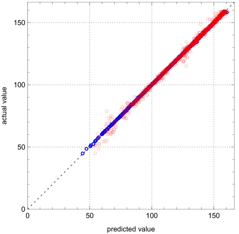
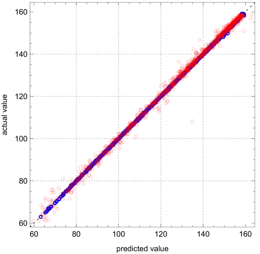
We use various initial conditions for $B(z,t=0)$ by holding the energy density fixed (in the appropriate units) to $2$. This corresponds to choosing the initial condition $a_{\text{n}}(t=0)=-1$. This ensures that all the initial conditions in the dataset thermalize at approximately the same time (because energy or equivalently the temperature sets the timescale of thermalization $t_{\text{th}}\approx 2$). We find that the learning of event horizon as well as apparent horizon areas happens almost perfectly at all times from the initial time until the time at which the system thermalizes.

Our main result is that training the neural network with only a handful of simple features of $b_{\text{n}}(t)$ time series suffices to generate predictions comparable to the predictions made by the neural network trained on the full $b_{\text{n}}(t)$ time series data. These simple features involve just the maximum and minimum values of the pressure anisotropy and the respective times when they are attained, the half width of the maxima and the minima, and the zeroes of the time series truncated at $t=3$. This data with such short input vectors restricted to a maximum length of $30$ (by truncating the last set of zeroes if needed) predicts both the event and apparent horizon areas (almost) perfectly at all times. It is to be noted that although the apparent horizon is determined causally unlike the event horizon, as should be obvious from our previous discussion, for the short input vector we should include data from times beyond the time at which the apparent horizon is being predicted simply because we are sparsifying the past data.

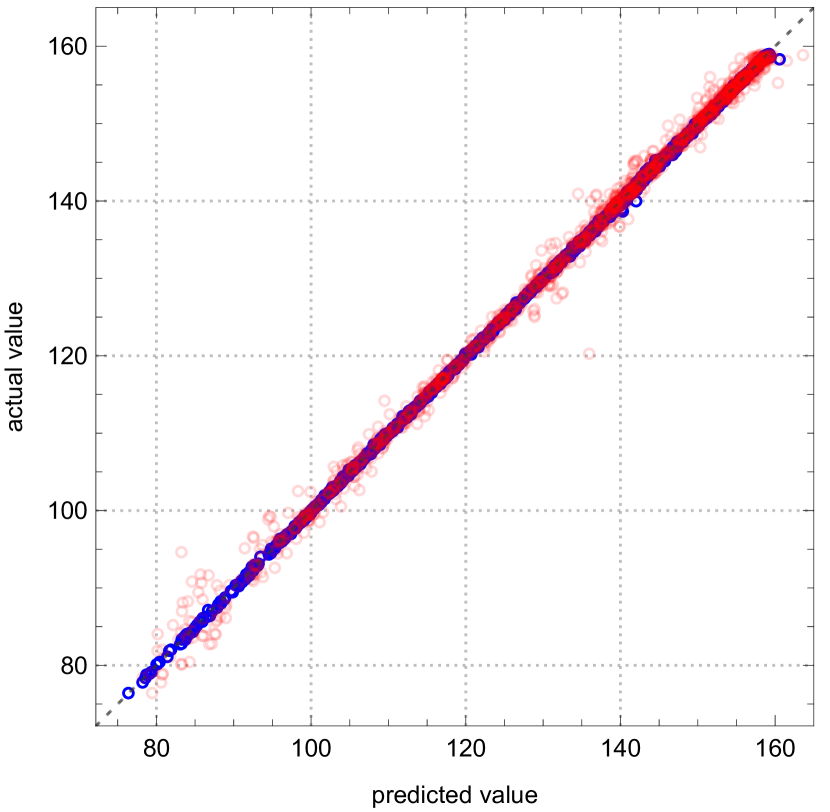
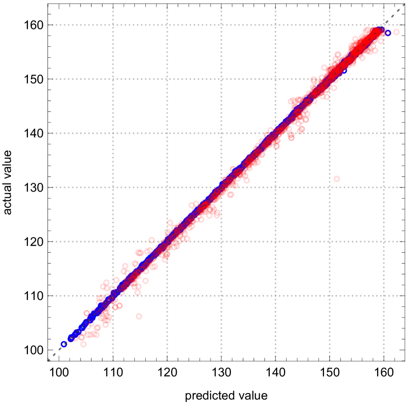
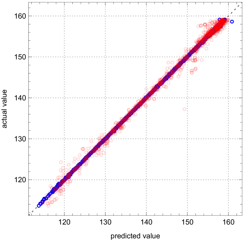
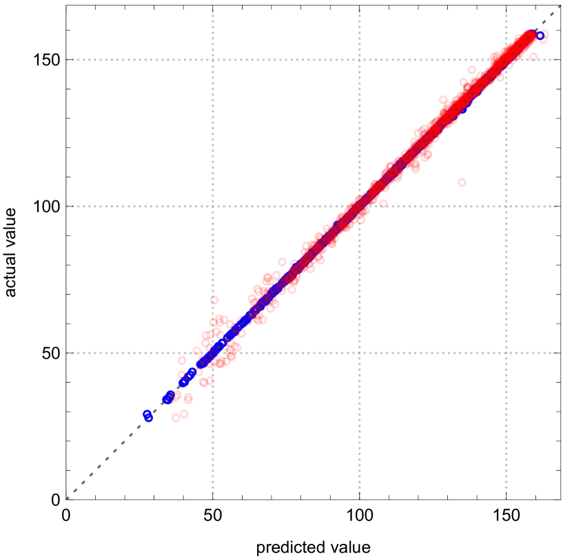
The details of the machine learning computation are given in Appendix B along with a statistical analysis of the results. Figure 1 gives representative plots.

(a) $S_{EH}$ at $t=0$

(b) $S_{EH}$ at $t=0.75$

(c) $S_{EH}$ at $t=1$

(d) $S_{AH}$ at $t=0$

(e) $S_{AH}$ at $t=0.75$

(f) $S_{AH}$ at $t=1$

Figure 1: Testing statistics for $S_{\text{EH}}$ and $S_{\text{AH}}$ with both long input vector (blue) as well as short input vector (red) at various times. Note that the scale is set by the (conserved) energy density which is the same for all the elements of the dataset used for machine learning, which makes it meaningful to compare the times across the dataset.

4 Discussion and outlook

In this letter, we have demonstrated that neural networks can learn some aspects of bulk geometry given simply the time series of a one-point function (expectation value of an operator) as input. In particular, we establish that the areas of the event and apparent horizons can be learned from the time series data of the pressure anisotropy in the boundary field theory. Furthermore, neural networks also predict the black hole entropies at all times from only a small number of features of the time series data, namely the values and half-widths of the maxima and minima, the times the latter are attained, and the times of the first zeroes with the maximum length of the input vector set to $30$ and with the time series truncated to a maximum value of time commensurate with the thermalization time.

Generally, in order to construct the bulk spacetime metric, one would need the boundary data and also initial conditions. In our work, we have considered a wide class of initial conditions, and we have demonstrated that machine learning of the event and apparent horizon entropies is possible not only without any inputs of the initial conditions but also with inputs of only compressed boundary data. These results are surprising and point to universality classes of bulk metrics and their dual states which can be characterized only by simple features of the time series of simple observables, namely one-point functions. Our work therefore indicates that neural networks are not only promising tools for addressing bulk reconstruction in AdS/CFT but also for obtaining new insights into holographic dynamics.

We argue that our approach can yield the holographic interpretation of the entropy functions obtained from the evolving event and apparent horizons in dynamical black hole geometries dual to non-equilibrium states. It is natural to think of entropy functions as determining simplistic statistical ensembles which can be constructed from simple inputs and which provide best approximations to all observables of a given state. In fact, a precise holographic interpretation of semiclassical spacetime itself as a minimum bias statistical ensemble has been advocated in Jafferis:2022wez . The event and apparent horizon entropies can be naturally thought of as further simplifications of the emergent spacetime.

The first step towards developing such a precise statistical interpretation of non-equilibrium event and apparent horizon entropies would be to test if machine learning of these entropy functions is possible without a detailed knowledge of the two-derivative gravity theory (Einstein’s theory coupled to a few bulk fields) governing the bulk dynamics in holographic duality. If the entropies can lead to a statistical ensemble which can approximate observables of the non-equilibrium state dual to the dynamical black hole geometry, the algorithm for obtaining such an ensemble should not depend on the specific details of the theory. Conversely, it should be possible to extract these entropy functions without detailed knowledge of the dual strongly interacting holographic theory.

Indeed the results of Joshi:2017ump strongly suggest that the entropy functions can be learnt from simple boundary data without detailed knowledge of the underlying microscopic theory or the dual bulk gravitational theory. It was shown in Joshi:2017ump that a simple Ads–Schwarzschild geometry with a time-dependent mass (viz., an Ads–Vaidya geometry) gives the best approximation to non-equilibrium causal correlation functions provided it reproduces the exact time-dependent apparent horizon entropy of the exact dual gravitational solution dual to the given state. Similarly, a simple Ads–Vaidya geometry gives the best approximation to coarse-grained features of non-equilibrium causal correlation functions provided it reproduces the exact time-dependent event horizon entropy of the exact dual gravitational solution dual to the given state. In both cases, the approximations are typically better than one percent on average. Such Ads–Vaidya geometries are natural gravitational analogues of thermal density matrices with just time-dependent temperatures (although not exactly equivalent to the latter) as their construction require only inputs of the entropy functions (and no knowledge of the dual gravitational theory). Our present work together with the results of Joshi:2017ump suggest that conversely the entropy functions can possibly be learnt from simple one-point functions without knowledge of the dual bulk two-derivative gravitational theory, and thus such entropy functions can be interpreted as measures of information which need to be extracted from one-point functions in order to construct quantum statistical ensembles that give best possible approximations to the dual states, especially for reproducing the two-point correlation functions. Our approach can be useful to arrive at such a precise interpretation.

In the future, we would like to unbox the neural network in order to understand how learning takes place, for instance, by employing techniques like layer-wise relevance propagation montavon2019layer ; Craven:2020bdz and this should be important for the stated goal of interpreting the entropy functions. Because this work is a proof of principle that we can apply Big Data techniques to holography and machine learn salient features of spacetime dynamics from dual data, we do not have a need to optimize the network hyperparameters to improve performance. It would be good to do this, of course.

Appendix A Feedforward neural networks

Consider the map

$$\begin{array}[]{cccc}f_{i}:&\mathbb{R}^{n_{i-1}}&\quad\to&\mathbb{R}^{n_{i}}\cr&\mathbf{v}_{i-1}&\quad\mapsto&\mathbf{v}_{i}=\sigma(\mathbf{v}_{i}^{\prime})\end{array}~{},$$ (14)

where $\mathbf{v}_{i}^{\prime}=W^{(i)}\cdot\mathbf{v}_{i-1}+\mathbf{b}_{i}$. The vector $\mathbf{b}_{i}\in\mathbb{R}^{n_{i}}$ is called a bias vector and the $n_{i}\times n_{i-1}$ matrix $W^{(i)}$ is called a weight matrix. The activation function $\sigma$ acts non-linearly elementwise on the components of the vector $\mathbf{v}_{i}^{\prime}$. In our case, we choose $\sigma(x)=x\,\Theta(x)$, where $\Theta(x)$ is the Heaviside step function. (This is the rectified linear unit or ReLU activation.) Taking the vector $\mathbf{v}_{\text{in}}:=\mathbf{v}_{0}\in\mathbb{R}^{n_{0}}$ as the input vector, this procedure is iterated:

$$\mathbf{v}_{\ell}=f_{\ell}(f_{\ell-1}(\cdots(f_{1}(\mathbf{v}_{0})\cdots)))~{},\qquad a_{\text{out}}:=\sum_{m=1}^{n_{\ell}}\mathbf{v}_{\ell}^{m}~{}.$$ (15)

In writing $a_{\text{out}}$, we have summed the components of the vector $\mathbf{v}_{\ell}$.

Suppose we have a set of input vectors labeled by $j$ that we use for training. To each of these input vectors $\mathbf{v}_{\text{in},j}$ we associate a target value $\alpha_{j}\in\mathbb{R}$. We then consider a mean squared loss function that compares each $\alpha_{j}$ to its predicted value $a_{\text{out},j}$. Backpropagation enables us to tune the elements of the weight matrices and bias vectors to minimize this loss. In this way, we have constructed an $\ell$-hidden layer fully connected feedforward neural network that is trained to approximate $\alpha_{j}$ from the features encoded in $\mathbf{v}_{\text{in},j}$ via stochastic gradient descent. The dimension $n_{i}$ specifies the number of neurons in the $i$-th hidden layer.

In our experiments, the architectures of the neural network are dependent on the vector $\mathbf{v}_{\text{in}}$. With long input vectors in $\mathbb{R}^{299}$, we use three hidden layers with $2000$ neurons each. With short input vectors in $\mathbb{R}^{30}$, we use three hidden layers with $150$ neurons each. (The input vectors are described in Appendix B.) We use $70\%$ of a $10000$ data points for training, $15\%$ for validation, and $15\%$ for testing. Performance statistics are reported on the test set. The neural networks are implemented in Mathematica Mathematica and use Adam for optimization. We make our code available on Github GitHub-ml-holo-23 .

Appendix B Data preparation and analysis

We use the following family of profiles for specifying the initial conditions of $B(z,t=0)$:

$$B(z,t=0)=z^{3}\left(\mathcal{R}_{1}e^{-200(z-0.2)^{2}}+\mathcal{R}_{2}e^{-200(z-0.5)^{2}}\mathcal{R}_{3}e^{-100(z-0.8)^{2}}\right)~{},$$ (16)

where $\mathcal{R}_{1,2,3}$ are (pseudo)random numbers between $0$ and $1$ and $z=L^{2}/r$. These profiles are superpositions of three Gaussians centered at $0.2$, $0.5$, and $0.8$, respectively. (The range of bulk radial coordinate $z$ is between $0$ and $1$ which includes the apparent horizon (and thus the event horizon as well) as we set $L=1$ and $a_{\text{n}}=-1$.) By varying $\mathcal{R}_{1,2,3}$, we generate various initial conditions. We use the characteristic method outlined in the main text to solve the Einstein equations wherein at each time step, a set of nested ordinary differential equations in radial coordinate $r$ (or equivalently $z$) are solved using the pseudospectral method Chesler:2013lia ; Boyd . In the pseudospectral method, the radial coordinate $r$ is discretized using a Chebyshev grid with a certain choice of the number of grid points, $n$. In our simulations, we have chosen $n=60$. The time updates are performed using the 4th order Adams–Bashforth method (see main text). This method requires knowing the values of the functions to be time evolved at previous four time steps. Therefore, for the first nine time steps, we use smaller time steps and perform numerical integration of the interpolated functions. From the 10th time step onwards, the 4th order Adams–Bashforth method is used for time stepping with the value of time step $\delta t=0.001$. The residual gauge freedom in (1) is fixed by setting the coefficient of $r$ in the near-boundary expansion of $A(r,t)$ in (4) to zero.

As described in the main text, we employ neural networks to make predictions of the areas of the event and the apparent horizons at various times. We observe that the (common) thermalization time ($t_{\text{th}}$) is approximately equal to $2$ (set by the energy density, i.e., $a_{\text{n}}$), so we choose $t=0,0.75,$ and $1$ as representative values. In each case, we train the neural network on the longer $b_{\text{n}}(t)$ time series data (referred to as a long input vector) as well as on the shorter data which retains only a handful of features of $b_{\text{n}}(t)$ time series data (referred to as a short input vector). More precisely, the long input vector is $b_{\text{n}}(t_{0}+k\delta t)$, where $\delta t=0.01$ and

$$k=(10^{-4},10^{-7/2},10^{-3},10^{-5/2},10^{-2},10^{-3/2},10^{-1},10^{-1/2},1-\sum_{i=-8}^{-1}10^{i/2})$$

for first nine time steps respectively and $k=1$ from 10th time step onward. (Although, we use time step $\delta t=0.001$ for the simulations that generate elements of our dataset, for the long input vector, we only keep values of various dynamical quantities with $\delta t=0.01$.) The full time series is truncated to $t=3$.

A short input vector contains a certain handful of features of the pressure anisotropy time series. The features of interest are:

1. $b_{\text{n},\text{max}}$: maximum value that $b_{\text{n}}(t)$ takes;

2. $t_{\text{max}}$: time $t$ when $b_{\text{n},\text{max}}$ is attained;

3. $b_{\text{n},\text{min}}$: minimum value that $b_{\text{n}}(t)$ takes;

4. $t_{\text{min}}$: time $t$ when $b_{\text{n},\text{min}}$ is attained;

5. full width at half maximum;

6. full width at half minimum ;

7. times corresponding to the zeroes of $b_{\text{n}}(t)$.

Note that the number of zeros of $b_{\text{n}}(t)$ is in general different for different initial conditions. Therefore we fix the maximum length of the input vector to $30$ by padding with zeroes on the right as necessary. Note also that the full time series is truncated to $t=3$.

To assess the performance of the neural network, we compute the following quantities over the test set:

$$\text{mean deviation}\;(\text{MD}): \text{Mean}[\frac{\text{Abs}[\text{actual}-\text{predicted}]}{\text{actual}}]~{},$$ (17)

$$\text{baseline}: \text{Mean}[\frac{\text{Abs}[\text{actual}-\text{Mean}[\text{actual}]]}{\text{actual}}]~{}.$$ (18)

The baseline (18) simply assigns the mean in the dataset as a universal prediction. The accuracy of the trained neural network is compared to this baseline. We as well calculate the standard deviation (SD) between the actual value and the predicted value, $R$-squared, and $\chi$-squared in the usual way. These statistics are reported in Tables 1 and 2.

time	input vector	MD	baseline	SD	$R$-squared	$\chi$-Squared
$t=0$	long	0.00126523	0.146794	0.226	1.00	0.579892
	short	0.005895	0.146794	1.20	0.997	19.1147
$t=0.75$	long	0.000825361	0.101556	0.161	1.00	0.273529
	short	0.003919	0.101556	1.00	0.996	11.5835
$t=1$	long	0.000615757	0.0820156	0.132	1.00	0.173059
	short	0.003297	0.0820156	0.882	0.995	8.5098

Table 1: Various statistical measures assessing performance of neural network for $S_{\text{EH}}$ prediction.

time	input vector	MD	baseline	SD	$R$-squared	$\chi$-Squared
$t=0$	long	0.00153455	0.249098	0.251	1.00	0.855986
	short	0.01143	0.249098	1.97	0.995	80.0903
$t=0.75$	long	0.00155447	0.197801	0.245	1.00	0.782011
	short	0.008481	0.197801	1.75	0.995	48.7921
$t=1$	long	0.00132608	0.18089	0.220	1.00	0.574205
	short	0.007935	0.18089	1.65	0.995	38.8055

Table 2: Various statistical measures assessing performance of neural network for $S_{\text{AH}}$ prediction.

Appendix C $k$-fold cross validation

As a further test of the robustness of predictive power of our neural networks trained on both long and short input data, we perform $k$-fold cross validation. In this method, one randomly divides the entire dataset into $k$ subsets (also called $k$ folds). Then, one keeps one of these $k$ folds as testing data and trains the neural network on the remaining $k-1$ folds. One repeats this $k$ times, each time choosing a different fold as the testing dataset and the corresponding remaining $k-1$ folds as the training dataset. Finally, one takes the average and standard deviation of all $k$ runs’ learning statistics. The most common choices of $k$ are $5$ or $10$. We chose $k=5$.

We find that the various statistical measures reported in tables 1 and 2 don’t vary much across $5$-folds. In particular $R$-squared stays $\sim 1$ and others also don’t deviate significantly from their mean value across $5$-folds which are close to their corresponding values reported in tables 1 and 2. We report the average values of each of the quantities of tables 1 and 2 across $5$-folds and also their standard deviation (SD) in the tables 3 and 4.

		$t=0$		$t=0.75$		$t=1$
		long	short	long	short	long	short
Average	MD	0.00096	0.0056	0.0008	0.1152	0.0010	0.0033
	baseline	0.1492	0.1492	0.1039	0.1039	0.0842	0.0842
	SD	0.1562	1.166	3.3286	0.9680	0.1820	0.8094
	$R$-squared	1	0.997	1	0.9964	0.9998	0.9964
	$\chi$-Squared	0.3914	22.6193	0.2696	14.282	0.6499	9.2986
SD	MD	0.00017	0.00045	0.0002	0.2484	0.0008	0.0002
	baseline	0.0020	0.0023	0.0017	0.0017	0.0015	0.0014
	SD	0.0219	0.1193	7.1395	0.1459	0.1299	0.0602
	$R$-squared	0	0.0007	0	0.0009	0.0004	0.0005
	$\chi$-Squared	0.1093	3.8048	0.1099	4.2840	0.8675	1.2762

Table 3: Average and standard deviation (SD) across $5$-folds (of cross validation) of various statistical measures assessing performance of neural network for $S_{\text{EH}}$ prediction

		$t=0$		$t=0.75$		$t=1$
		long	short	long	short	long	short
Average	MD	0.0018	0.0127	0.0021	0.0081	0.0014	0.0075
	baseline	0.2535	0.2535	0.2009	0.2009	0.1853	0.1853
	SD	0.2650	2.09	0.3042	1.532	0.229	1.48
	$R$-squared	1	0.9948	1	0.9966	1	0.9964
	$\chi$-Squared	1.4144	128.4	2.8488	52.15	0.8975	41.346
SD	MD	0.0004	0.0021	0.001	0.0005	0.0002	0.0011
	baseline	0.0038	0.0038	0.0059	0.0032	0.0045	0.0035
	SD	0.0514	0.3253	0.1357	0.1076	0.037	0.2513
	$R$-squared	0	0.0019	0	0.0005	0	0.0015
	$\chi$-Squared	0.5181	51.11	2.4119	10.184	0.295	13.927

Table 4: Average and standard deviation (SD) across $5$-folds (of cross validation) of various statistical measures assessing performance of neural network for $S_{\text{AH}}$ prediction

References

- (1) G. ’t Hooft, Dimensional reduction in quantum gravity, Conf. Proc. C 930308 (1993) 284–296. arXiv:gr-qc/9310026.
- (2) L. Susskind, The World as a hologram, J. Math. Phys. 36 (1995) 6377–6396. arXiv:hep-th/9409089, doi:10.1063/1.531249.
- (3) J. M. Maldacena, The Large N limit of superconformal field theories and supergravity, Adv. Theor. Math. Phys. 2 (1998) 231–252. arXiv:hep-th/9711200, doi:10.4310/ATMP.1998.v2.n2.a1.
- (4) S. S. Gubser, I. R. Klebanov, A. M. Polyakov, Gauge theory correlators from noncritical string theory, Phys. Lett. B 428 (1998) 105–114. arXiv:hep-th/9802109, doi:10.1016/S0370-2693(98)00377-3.
- (5) E. Witten, Anti-de Sitter space and holography, Adv. Theor. Math. Phys. 2 (1998) 253–291. arXiv:hep-th/9802150, doi:10.4310/ATMP.1998.v2.n2.a2.
- (6) T. Banks, W. Fischler, S. H. Shenker, L. Susskind, M theory as a matrix model: A Conjecture, Phys. Rev. D 55 (1997) 5112–5128. arXiv:hep-th/9610043, doi:10.1103/PhysRevD.55.5112.
- (7) D. Harlow, TASI Lectures on the Emergence of Bulk Physics in AdS/CFT, PoS TASI2017 (2018) 002. arXiv:1802.01040, doi:10.22323/1.305.0002.
- (8) T. Kibe, P. Mandayam, A. Mukhopadhyay, Holographic spacetime, black holes and quantum error correcting codes: a review, Eur. Phys. J. C 82 (5) (2022) 463. arXiv:2110.14669, doi:10.1140/epjc/s10052-022-10382-1.
- (9) K. Hashimoto, S. Sugishita, A. Tanaka, A. Tomiya, Deep Learning and Holographic QCD, Phys. Rev. D 98 (10) (2018) 106014. arXiv:1809.10536, doi:10.1103/PhysRevD.98.106014.
- (10) K. Hashimoto, S. Sugishita, A. Tanaka, A. Tomiya, Deep learning and the AdS/CFT correspondence, Phys. Rev. D 98 (4) (2018) 046019. arXiv:1802.08313, doi:10.1103/PhysRevD.98.046019.
- (11) K. Hashimoto, AdS/CFT correspondence as a deep Boltzmann machine, Phys. Rev. D 99 (10) (2019) 106017. arXiv:1903.04951, doi:10.1103/PhysRevD.99.106017.
- (12) H.-Y. Hu, S.-H. Li, L. Wang, Y.-Z. You, Machine Learning Holographic Mapping by Neural Network Renormalization Group, Phys. Rev. Res. 2 (2) (2020) 023369. arXiv:1903.00804, doi:10.1103/PhysRevResearch.2.023369.
- (13) J. Tan, C.-B. Chen, Deep learning the holographic black hole with charge, Int. J. Mod. Phys. D 28 (12) (2019) 1950153. arXiv:1908.01470, doi:10.1142/S0218271819501530.
- (14) Y.-K. Yan, S.-F. Wu, X.-H. Ge, Y. Tian, Deep learning black hole metrics from shear viscosity, Phys. Rev. D 102 (10) (2020) 101902. arXiv:2004.12112, doi:10.1103/PhysRevD.102.101902.
- (15) T. Akutagawa, K. Hashimoto, T. Sumimoto, Deep Learning and AdS/QCD, Phys. Rev. D 102 (2) (2020) 026020. arXiv:2005.02636, doi:10.1103/PhysRevD.102.026020.
- (16) K. Hashimoto, H.-Y. Hu, Y.-Z. You, Neural ordinary differential equation and holographic quantum chromodynamics, Mach. Learn. Sci. Tech. 2 (3) (2021) 035011. arXiv:2006.00712, doi:10.1088/2632-2153/abe527.
- (17) M. Song, M. S. H. Oh, Y. Ahn, K.-Y. Kima, AdS/Deep-Learning made easy: simple examples, Chin. Phys. C 45 (7) (2021) 073111. arXiv:2011.13726, doi:10.1088/1674-1137/abfc36.
- (18) K. Hashimoto, K. Ohashi, T. Sumimoto, Deriving the dilaton potential in improved holographic QCD from the meson spectrum, Phys. Rev. D 105 (10) (2022) 106008. arXiv:2108.08091, doi:10.1103/PhysRevD.105.106008.
- (19) J. Lam, Y.-Z. You, Machine learning statistical gravity from multi-region entanglement entropy, Phys. Rev. Res. 3 (4) (2021) 043199. arXiv:2110.01115, doi:10.1103/PhysRevResearch.3.043199.
- (20) K. Li, Y. Ling, P. Liu, M.-H. Wu, Learning the black hole metric from holographic conductivity, Phys. Rev. D 107 (6) (2023) 066021. arXiv:2209.05203, doi:10.1103/PhysRevD.107.066021.
- (21) P. Kumar, T. Mandal, S. Mondal, Black Holes and the loss landscape in machine learning, JHEP 10 (2023) 107. arXiv:2306.14817, doi:10.1007/JHEP10(2023)107.
- (22) K. Hashimoto, K. Ohashi, T. Sumimoto, Deriving the dilaton potential in improved holographic QCD from the chiral condensate, PTEP 2023 (3) (2023) 033B01. arXiv:2209.04638, doi:10.1093/ptep/ptad026.
- (23) R. Katsube, W.-H. Tam, M. Hotta, Y. Nambu, Deep learning metric detectors in general relativity, Phys. Rev. D 106 (4) (2022) 044051. arXiv:2206.03006, doi:10.1103/PhysRevD.106.044051.
- (24) C. Park, S. Kim, J. H. Lee, Holography Transformer (11 2023). arXiv:2311.01724.
- (25) V. Balasubramanian, P. Kraus, A Stress tensor for Anti-de Sitter gravity, Commun. Math. Phys. 208 (1999) 413–428. arXiv:hep-th/9902121, doi:10.1007/s002200050764.
- (26) S. de Haro, S. N. Solodukhin, K. Skenderis, Holographic reconstruction of space-time and renormalization in the AdS / CFT correspondence, Commun. Math. Phys. 217 (2001) 595–622. arXiv:hep-th/0002230, doi:10.1007/s002200100381.
- (27) S. Bhattacharyya, S. Minwalla, Weak Field Black Hole Formation in Asymptotically AdS Spacetimes, JHEP 09 (2009) 034. arXiv:0904.0464, doi:10.1088/1126-6708/2009/09/034.
- (28) L. K. Joshi, A. Mukhopadhyay, F. Preis, P. Ramadevi, Exact time dependence of causal correlations and nonequilibrium density matrices in holographic systems, Phys. Rev. D 96 (10) (2017) 106006. arXiv:1704.02936, doi:10.1103/PhysRevD.96.106006.
- (29) P. M. Chesler, L. G. Yaffe, Numerical solution of gravitational dynamics in asymptotically anti-de Sitter spacetimes, JHEP 07 (2014) 086. arXiv:1309.1439, doi:10.1007/JHEP07(2014)086.
- (30) W. van der Schee, Gravitational collisions and the quark-gluon plasma, Ph.D. thesis, Utrecht U. (2014). arXiv:1407.1849.
- (31) K. Skenderis, Lecture notes on holographic renormalization, Class. Quant. Grav. 19 (2002) 5849–5876. arXiv:hep-th/0209067, doi:10.1088/0264-9381/19/22/306.
- (32) R. L. Arnowitt, S. Deser, C. W. Misner, Dynamical Structure and Definition of Energy in General Relativity, Phys. Rev. 116 (1959) 1322–1330. doi:10.1103/PhysRev.116.1322.
- (33) P. M. Chesler, L. G. Yaffe, Horizon formation and far-from-equilibrium isotropization in supersymmetric Yang-Mills plasma, Phys. Rev. Lett. 102 (2009) 211601. arXiv:0812.2053, doi:10.1103/PhysRevLett.102.211601.
- (34) I. Booth, M. P. Heller, G. Plewa, M. Spalinski, On the apparent horizon in fluid-gravity duality, Phys. Rev. D 83 (2011) 106005. arXiv:1102.2885, doi:10.1103/PhysRevD.83.106005.
- (35) N. Engelhardt, A. C. Wall, Decoding the Apparent Horizon: Coarse-Grained Holographic Entropy, Phys. Rev. Lett. 121 (21) (2018) 211301. arXiv:1706.02038, doi:10.1103/PhysRevLett.121.211301.
- (36) S. W. Hawking, Gravitational radiation from colliding black holes, Phys. Rev. Lett. 26 (1971) 1344–1346. doi:10.1103/PhysRevLett.26.1344.
- (37) R. M. Wald, The thermodynamics of black holes, Living Rev. Rel. 4 (2001) 6. arXiv:gr-qc/9912119, doi:10.12942/lrr-2001-6.
- (38) R. Bousso, A Covariant entropy conjecture, JHEP 07 (1999) 004. arXiv:hep-th/9905177, doi:10.1088/1126-6708/1999/07/004.
- (39) R. Bousso, Z. Fisher, S. Leichenauer, A. C. Wall, Quantum focusing conjecture, Phys. Rev. D 93 (6) (2016) 064044. arXiv:1506.02669, doi:10.1103/PhysRevD.93.064044.
-
(40)
P. Mehta, M. Bukov, C.-H. Wang, A. G. Day, C. Richardson, C. K. Fisher, D. J.
Schwab, A high-bias,
low-variance introduction to machine learning for physicists, Physics
Reports 810 (2019) 1–124.
doi:10.1016/j.physrep.2019.03.001.
URL https://doi.org/10.1016%2Fj.physrep.2019.03.001 - (41) F. Ruehle, Data science applications to string theory, Phys. Rept. 839 (2020) 1–117. doi:10.1016/j.physrep.2019.09.005.
- (42) D. L. Jafferis, D. K. Kolchmeyer, B. Mukhametzhanov, J. Sonner, Jackiw-Teitelboim gravity with matter, generalized eigenstate thermalization hypothesis, and random matrices, Phys. Rev. D 108 (6) (2023) 066015. arXiv:2209.02131, doi:10.1103/PhysRevD.108.066015.
- (43) S. Banerjee, T. Ishii, L. K. Joshi, A. Mukhopadhyay, P. Ramadevi, Time-dependence of the holographic spectral function: Diverse routes to thermalisation, JHEP 08 (2016) 048. arXiv:1603.06935, doi:10.1007/JHEP08(2016)048.
- (44) G. Montavon, A. Binder, S. Lapuschkin, W. Samek, K.-R. Müller, Layer-wise relevance propagation: an overview, in: Explainable AI: interpreting, explaining and visualizing deep learning, Springer, 2019, pp. 193–209.
- (45) J. Craven, V. Jejjala, A. Kar, Disentangling a deep learned volume formula, JHEP 06 (2021) 040. arXiv:2012.03955, doi:10.1007/JHEP06(2021)040.
(46)
W. R. Inc., Mathematica, Version
13.3, champaign, IL, 2023.
URL https://www.wolfram.com/mathematica -
(47)
V. Jejjala, S. Mondkar, A. Mukhopadhyay, R. Raj,
Ml-holo (2023).
URL https://github.com/sukrut123/ML-Holo - (48) J. Boyd, Chebyshev and Fourier Spectral Method, Springer (1989). doi:0176-5035.