A star under multiple influences

Abstract

Context. Close binaries with magnetically active components are astrophysical laboratories for studying the effects of binarity on activity. Of particular interest are binary and multiple star systems that contain a solar-type active component with an internal structure similar to the Sun, allowing us to study how the dynamo of a solar-type star would work under different conditions.

Aims. We are conducting a comprehensive investigation of V815 Her using photometric and spectroscopic data to understand the origin of the activity and what influences it in the short and long term.

Methods. Using space photometry we performed light curve modeling in order to derive astrophysical and orbital parameters for the eclipsing binary subsystem V815 Her B. Using archival photometric data covering a century we carried out a time frequency analysis.Spectral synthesis was applied to determine the basic astrophysical parameters of the rapidly rotating primary using high-resolution STELLA spectra recorded in 2018.

Results. Photometric analysis of archived data revealed multiple cycles on timescales between $\sim$6.5 and $\sim$26 years, some of which may be harmonic. From TESS photometry we obtained orbital solution for the V815 Her B subsystem. By placing the primary component on the Hertzsprung$-$Russell-diagram, we can deduce an age of $\approx$30 Myr, in line with the high Li-6707 abundance. The STELLA spectra covering the  200 day-long observing season enabled to create 19 time-series Doppler images, which revealed a constantly changing spotted surface on a time scale of a few weeks. From the consecutive image pairs we built up the average cross-correlation function map to measure the surface differential rotation of the spotted star, from which we derive a weak solar-type surface shear.

Conclusions. We found evidence that the V815 Her B component previously apostrophized as a ’third body’ is actually an eclipsing close binary subsystem of two M dwarfs with a period of 0.5 d, i.e., V815 Her is a 2+2 hierarchical quadruple system. The system is apparently young, only a few times ten million years old, consistent with the spotted primary V815 Her Aa being a zero-age main sequence star. Spot activity on the primary was found to be vivid. Fast starspot decay suggests that convective-turbulent erosion plays a more significant role in such a rapidly rotating star. The weak surface shear of V815 Her Aa due to differential rotation is presumably confined by tidal forces of the close companion V815 Her Ab. The slowly increasing photometric cycle of about 6.5 years on average is interpreted as a spot cycle of V815 Her Aa, which is probably modulated by the eccentric wide orbit.

1 Introduction

Close binaries that contain magnetically active components may be regarded as astrophysical laboratories for studying the effect of binarity on activity. Tidal forces in such systems are supposed to modify the operation of the magnetic dynamo, by altering the flux emergence patterns at the surface (Holzwarth & Schüssler 2003a, b). Amplified dynamo operation is expected, for instance, when fast rotation is sustained by weakening magnetic braking through angular momentum transport in a close binary system (Song et al. 2018). Although, other binarity-related effects like early-evolution accretion processes can also result in faster rotation (Meibom et al. 2007). In all probability, the gravitational influence of a close companion can suppress the differential rotation of the convection zone (Scharlemann 1982; Collier Cameron 2007) or even force the formation of active longitudes at certain phases fixed to the orbit (Oláh 2006; Kővári et al. 2021). Especially interesting are those binaries and multiple star systems which contain active G-type main-sequence (MS) stars with inner structure (convective zone) similar to that of the Sun, making it possible to investigate how the solar-type dynamo would work under different circumstances.

In accordance with the above, this time we choose the active G dwarf component of the single-lined but in fact a quaternary star system V815 Her (=HD 166181) for our study. In the beginning, it was believed that the G star with its enhanced magnetic activity inferred from strong Ca ii H&K emission is the primary member of a single-lined binary (SB1) system with an orbital period of $\approx$1.81 days (Nadal et al. 1974). Later using new spectroscopic data taken in 1992 at Kitt Peak National Observatory Dempsey et al. (1996) found a significant radial velocity difference of 11 kms^-1 compared to the data of Nadal et al. (1974), which was attributed to a possible third body with an orbital period of many years. This idea was warmed up by Fekel (2004) who, using new observations from 2002, calculated long-period orbital elements for the outer companion in the system for the first time with a preliminary period of 6.3 yr. With additional radial velocity measurements from 2003, this value was soon refined to 2092.2$\pm$5.8 d (Fekel et al. 2005). From their mass estimates for the system components of the long-period orbit Fekel et al. (2005) also suggested that the unseen component might also be a close binary. An important step forward in the story was that the outer component has been resolved by direct imaging within the frame of Gemini Deep Planet Survey (GDPS) by Lafrenière et al. (2007) who confirmed the astrometric solution of Fekel et al. (2005) for the third body. Going even further, in our paper we present space photometry from NASA’s Transiting Exoplanet Survey Satellite (TESS) to demonstrate that the suspected third body itself is indeed an eclipsing close binary system of two unseen but very likely M dwarfs, i.e. V815 Her is in fact a four-star system consisting of two close binaries orbiting each other.

According to photometric observations, it has long been known that the G (most probably G5-G6) active component features cool spots on its surface (Mekkadan et al. 1980). Strassmeier et al. (1989) reported automatic photoelectric telescope (APT) data from 1984-1986 in $U$, $B$ and $V$ colours and found that the photometric period associated to the rotation of the G star was 1.8195 d and 1.8356 d for 1985 and 1986, respectively, i.e. $\approx$1% longer than the orbital period from Nadal et al. (1974). From an extended study using long-term APT data taken in $BV$ between 1984 and 1998 Jetsu et al. (2000) found seasonal photometric period changes attributable to surface differential rotation of the spotted star. In addition, their time-series analysis revealed that one dominant active longitude was present for the full 14 year-long observing period while another weaker one emerged during some of the seasons. This APT data were re-analyzed in Savanov (2009) to reconstruct temperature inhomogeneities of the stellar surface. Again, two active longitudes were found, separated by about 0.5 rotation phase (cf. Jetsu et al. 2000), showing the so-called flip-flop phenomenon, i.e. when dominance switches quasi-periodically from one active longitude to the other.

Like the photosphere, the chromosphere and corona of the G component show the signatures of strong magnetic activity over a wide range of the electromagnetic spectrum. In addition to the strong and narrow Ca ii H&K emission (Nadal et al. 1974; Bopp 1984) $UV$ observations from the IUE satellite (Fekel et al. 1986) also indicate an active chromosphere. The absolute luminosity in the Mg ii k line supports this enhanced activity (Cardini et al. 2003), however, the lack of hot component in the $UV$ spectra suggests that the companions without contribution should be M-dwarfs or fainter. Moreover, the G star performs extreme-ultraviolet (EUV) radiation measured during the ROSAT Wide Field Camera All-Sky Survey (Pounds et al. 1993) and by the Extreme Ultraviolet Explorer satellite (Malina et al. 1994). Due to the ROSAT mission, V815 Her is known for its bright X-ray corona (Dempsey et al. 1993a, b). Indeed, its coronal luminosity of $L_{X}$=3.183 10³⁰ erg (Makarov 2003) classifies V815 Her as one of the 100 brightest stellar X-ray sources within 50 pc. Accordingly, with such an active corona, the star is known as a radio source as well (Drake et al. 1992).

V815 Her is not associated with any particular moving group (but see Wichmann et al. 2003, who cited the star as Pleiades-like). The strong Li line in the optical spectrum (Fekel et al. 2005) indicates that the G component is indeed young, near the zero-age main sequence (ZAMS). This observation is consistent with the star being listed in the Two Micron All Sky Survey Point Source Catalog (2MASS/PSC, Haakonsen & Rutledge 2009) due to its infrared excess, most probably related to primordial protoplanetary material.

In our paper, we perform a Doppler imaging study for the G star for the first time with reconstructing 19 time-series Doppler images using high-resolution optical spectra taken during a 9-month long observing run in 2018. The paper is organized as follows. In Sect. 2 we present the analysis of photometric data. Using TESS observations we analyze the newly discovered eclipses and give an orbital solution for the unseen, but most likely M+M dwarf binary companion V815 Her B in the quadruple system. In Sect. 3 we derive precise astrophysical parameters of the active G component for the Doppler imaging study presented in Sect. 4. Results are discussed in Sect. 5, and summarized in Sect. 6.

2 Photometric data and analysis

2.1 New light curve and orbital solution for V815 Her B using TESS data

TESS has observed V815 Her during sectors 26, 40 and 53. The sector 26 observations were carried out in 2-min cadence mode, so the light curves produced by the Science Processing Operations Center (SPOC) became directly available, while the Year 3 observations were carried out only in the 600-min cadenced full frame image (FFI) mode. Hence, we downloaded the 2-min cadence Pre-search Data Conditioned Simple Aperture Photometry (PDCSAP) data from the Mikulski Archive for Space Telescopes, while we processed the sector 40 and 53 FFI data with the software package Fitsh (Pál 2012). V815 Her (=TIC 320959269) is listed as a TESS planet host candidate with a supposed planetary orbit of 0.26 d. However, from a closer inspection, after removing the spot variability of the G star using the 1.8 d rotational period, it became clear to us that the depths of successive minima are slightly different, i.e., primary and secondary minima alternate. Evidently, instead of a planet orbiting with a period of 0.26 d we found a close eclipsing binary with a double-length period of 0.52 d bound to V815 Her A in the wide orbit.

To prepare data for the computation of the orbital solution of this new close binary we fitted the spotted light curve of the G star with a time-series three-spot model (see Fig. 1), which could properly follow the ever-changing light variation instead of a constant rotational period and its harmonics. For the fit we used an upgraded version of the SpotModeL code originally presented in Ribárik et al. (2003). For the light curve modeling the fixed parameters used were only crudely approximated (temperature, limb darkening, etc.) since the main goal was only to fit the light curve as smoothly as possible. The data were also cleaned from obvious outliers and a possible flare. The resulting model was subtracted from the original data and binned to 0.005 days (7.2 minutes) which was then used for binary modeling.

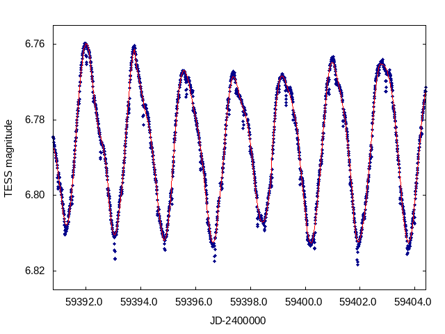
Figure 1: TESS sector 40 light curve of V815 Her (blue dots) fitted with a time-series three-spot model (red line).

For the eclipsing binary (EB) light curve modeling the residual curves of the three TESS sectors were converted into the flux domain, and normalized to unity. Then they were phase-folded with the previously determined eclipsing period of $0\aas@@fstack{d}5206$-day and binned into 500 evenly spaced phase cells. The fluxes in each cell were simply averaged, and these 500 mean flux values were rendered to the mid-phase moments of each cell. In such a manner we obtained evenly spaced, folded, binned, mean light curves separately for sectors 26, 40 and 53, which are plotted in Fig. 2.

The EB light curve analyses of these prepared data sets were carried out with software package Lightcurvefactory (see Borkovits et al. 2019, 2020, and further references therein). We analysed the data of the three sectors separately. During our MCMC-based parameter search process seven light curve parameters were adjusted, as follows: the total duration of an eclipse (which is a direct observable, and closely relates to the sum of the fractional radii of the two stars); the $R_{\mathrm{Bb}}/R_{\mathrm{Ba}}$ ratio of the stellar radii; the $T_{\mathrm{Ba}}$ effective temperature of the primary; the logarithm of the ratio of the effective temperatures $\log(T_{\mathrm{Bb}}/T_{\mathrm{Ba}})$; the “third” light $\ell$, which allows us to take into account the light contamination caused by the much brighter binary V815 Her A; the EB’s inclination $i_{\mathrm{B}}$ and, finally, the $T_{0}$ time of the reference epoch. Regarding the other orbital elements, the folded mean light curve in Fig. 2 reveals that the secondary eclipses occur just at (or, at least, very close to) phase 0.5, i.e. in the mid-times between the consecutive primary eclipses and, moreover, their durations look similar than that of the primary ones. Thus, we assume a circular EB orbit and, hence, keep the eccentricity fixed to $e_{\mathrm{B}}=0$.

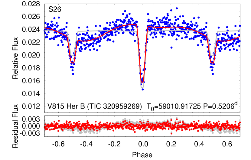
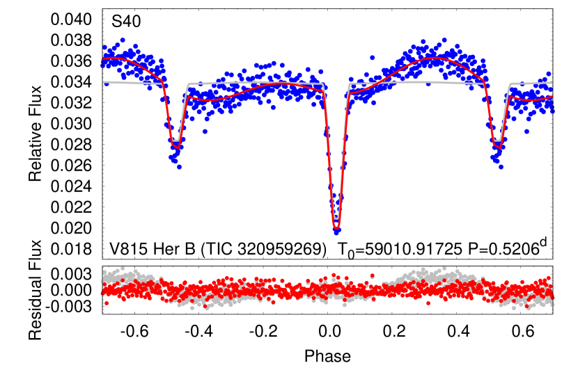
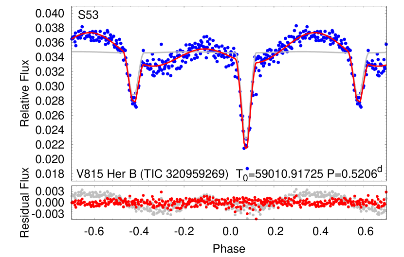
Figure 2: Cleaned and folded TESS Sector 26, 40 and 53 light curves (blue dots) for the wide binary companion V815 Her B. The original orbital solutions without assuming surface inhomogeneities are drawn with grey lines, while the models drawn with red lines fit also the light curve variations arising from stellar spots. The residuals of both fits are plotted on the bottom parts of all panels. Note, that the eclipses in sectors 40 and 53 (middle and bottom panels) shifted from phase 0.0 and 0.5 indicating timing variations which is discussed in the text in detail.

The adjustment of the effective temperature of the primary $T_{\mathrm{Ba}}$ needs some further explanation. In general, in the case of a single photometric band EB light curve, the temperature ratio of the two stars is well determined, while the effective temperatures of each star, themselves, play only a minor role in forming the light curve and hence, they are ill-determined. So, the usual treatment is to take one of the temperatures from some outer sources (e.g. spectroscopy or SED analysis), and to keep it fixed. However, in the present case, $T_{\mathrm{Ba}}$ was treated as a free parameter in order to check the physical reliability and consistency of our solution. This was done as follows. We know that the brighter binary should be a very young object. We reasonably assume that the two binaries are coeval, and thus, the two stars of binary B locate also on (or, very near to) the zero-age main sequence. Hence, we expect that the empirical mass–luminosity and mass–radius relations of Tout et al. (1996) are applicable for these stars. Therefore, with the combined and inverted use of these relations, we can compute the stellar masses and the radii, as well, from the effective temperatures. Then we can compare the total mass of binary B, obtained from our analysis to the minimum mass inferred from the RV solution of Fekel et al. (2005). Moreover, we can compare the stellar radii, calculated directly through the $M-R$ relations of Tout et al. (1996) to that calculated from the combination of the fractional radii (which are direct outputs of the light curve analysis) and the masses, inferred again from the Tout et al. (1996) relations.

Finally, we also note, that a first inspection of the folded, mean light curve of binary B reveals that despite the averaging over $\sim$25 orbital cycles, the out-of-eclipse light variations did not average out perfectly. One possible origin of these out-of-eclipse light variations might be the surface brightness inhomogeneities (e.g. stellar spots), which, for the (almost) synchronized stellar rotations may have ‘survived’ the averaging for the orbital period. We model these variations together with the EB light curve modeling simultaneously in a purely mathematical way, i.e. independent of their real origin, as follows. In each trial step, after the removal of the model EB light curve from the input light curve data, the residual is modelled with harmonic functions of two fixed frequencies (namely, the twice of the orbital frequency and, the orbital frequency itself), of which the four (plus one) coefficients are obtained via matrix inversion. Then, this mathematical model of the residual light curve is added to the EB model light curve and the actual $\chi^{2}$ value is calculated for this mixed model curve.

Table 1: Adjusted and derived astrophysical and orbital parameters for V815 Her B.

Orbital elements
$P$ [d]	$0.5206$
$a$ [$R_{\odot}$]	$2.33_{-0.24}^{+0.29}$
$e$	$0$
$\omega$ [∘]	…
$i$ [∘]	$89.17_{-1.45}^{+0.69}$
$T_{0}-2400000$ [d]	$59010.9173_{-0.0002}^{+0.0002}$
mass ratio $(q=m_{\mathrm{sec}}/m_{\mathrm{pri}})$	$0.48_{-0.08}^{+0.12}$
Stellar parameters
	Ba	Bb
Relative quantities
fractional radius [$R/a$]	$0.1603_{-0.0057}^{+0.0046}$	$0.1102_{-0.0060}^{+0.0053}$
temperature relative to $(T_{\mathrm{eff}})_{\mathrm{Ba}}$	$1$	$0.8736_{-0.0293}^{+0.0222}$
fractional flux (in TESS-band)	$0.0179_{-0.0021}^{+0.0020}$	$0.0038_{-0.0003}^{+0.0003}$
Physical quantities
$m$ [$M_{\odot}$]	$0.444_{-0.158}^{+0.198}$	$0.185_{-0.022}^{+0.053}$
$R$ [$R_{\odot}$]	$0.377_{-0.051}^{+0.047}$	$0.256_{-0.023}^{+0.026}$
$T_{\mathrm{eff}}$ [K]	$3702_{-174}^{+369}$	$3245_{-91}^{+174}$
$L_{\mathrm{bol}}$ [$L_{\odot}$]	$0.024_{-0.010}^{+0.019}$	$0.007_{-0.002}^{+0.003}$
$M_{\mathrm{bol}}$ [mag]	$8.77_{-0.64}^{+0.54}$	$10.20_{-0.41}^{+0.34}$
$M_{V}$ [mag]	$10.47_{-1.31}^{+1.04}$	$13.20_{-0.41}^{+0.34}$
$\log g$ (in cgs)	$4.94_{-0.08}^{+0.05}$	$4.91_{-0.06}^{+0.07}$
extra flux (in TESS-band)	$0.978_{-0.002}^{+0.002}$

In Table 1 we tabulate the median values and the $1\sigma$ statistical uncertainties of the parameters (including several derived, physical ones) that were obtained from our analysis for the sector 26 data. We also display the synthetic model fits (both with and without the mathematically modelled out-of-eclipse light variations) derived from the best-fit solution in Fig. 2. We note that in case of the analysis of sector 40 and 53 light curves we obtained mostly similar parameters within the tabulated 1-$\sigma$ uncertainties and, hence, we do not tabulate these results separately. The two exceptions are the $\ell$ extra flux and the $T_{0}$ epoch of the primary minimum. Regarding the former one, in sectors 40 and 53 we obtained smaller $\ell$ parameters with $\sim$5$-$10%, which we explain with a smaller level of contaminated fluxes in the TESS pixels. What physically more interesting is, the shift of the phase of the primary eclipses, which can also be seen in the consecutive panels of Fig. 2. In order to understand the nature and origin of this effect, we carried out a detailed analysis of the times of eclipsing minima.

2.2 Eclipse timing variation analysis of V815 Her B

We determined mid-eclipse times for all the observed primary and secondary eclipses of V815 Her B for the available TESS cleaned time-series (see in Sect. 2.1). The individual times of minima are tabulated in Table 5 of Appendix A. We derived an eclipse timing variation (ETV) curve using the linear ephemeris

$$\mathrm{MIN}_{\mathrm{I}}=2459010.917986+0.520647\times E,$$ (1)

where the zero epoch is given in barycentric Julian Days (BJD). We plot the obtained ETV curve in Fig. 3. As one can see, the ETV curve displays clearly a non-linear behaviour, which reveals that the observed eclipsing period is varying.

As a next step, we demonstrate that this variation can be explained by the light-travel time effect (LTTE) caused by the revolution of the eclipsing binary V815 Her B around its brighter counterpart V815 Her A, and the parameters of this LTTE orbit is in accordance with the former RV solution of Fekel et al. (2005). This indicates, that this currently discovered EB is identical with the third component suspected formerly through RV measurements. In order to demonstrate this fact, we derive LTTE solution from the outer RV orbit of Fekel et al. (2005, their Table 2). While doing so, one should be cautious about a few things. First, the argument of pericenter of the outer orbit ($\omega_{\mathrm{A}}$) given in the RV solution refers to the orbit of component A, while in the LTTE solution of component B, the argument of pericenter of component B ($\omega_{\mathrm{B}}=\omega_{\mathrm{A}}+180^{\mathrm{o}}$) is present. Moreover, the projected semi-major axis $a_{\mathrm{A}}\sin i_{\mathrm{out}}$ of the orbit of component A around the center of mass of the whole quadruple system, which was deduced from the amplitude of the RV curve, should also be transformed to the projected semi-major axis of component B ($a_{\mathrm{B}}\sin i_{\mathrm{out}}=m_{\mathrm{A}}/m_{\mathrm{B}}\times a_{\mathrm{A}}\sin i_{\mathrm{out}}$). For this step, we must know the mass ratio of the two binaries. For the formerly known, brighter component we accept $m_{\mathrm{A}}=m_{\mathrm{Aa}}+m_{\mathrm{Ab}}=1.27\,M\sun$ (Fekel et al. 2005), while our solution gives the mass of component B to be $m_{\mathrm{B}}=m_{\mathrm{Ba}}+m_{\mathrm{Bb}}=0.63\,M\sun$, which results in an outer mass ratio of $m_{\mathrm{A}}/m_{\mathrm{B}}=2.02$. Taking into account these constraints, and plotting the theoretical ETV curve against the measured ones, one can see a nice agreement (see Fig. 3), which, in our readings demonstrate nicely that the spectroscopic multiplicity of V815 Her is confirmed independently through TESS photometry, and the third spectroscopic component itself is a close, eclipsing binary, forming such a way a close quadruple system with a 2+2 hierarchy.

For comparison, the periods and geometrical parameters of the wide (V815 Her AB) and the two close orbits (V815 Her A and B) in the 2+2 hierarchical system are given in Table 2.

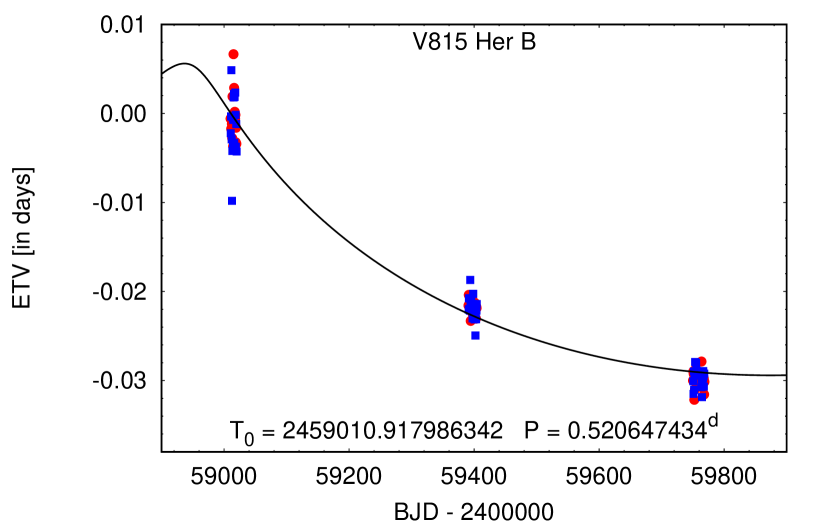
Figure 3: Eclipse timing variations of V815 Her B, calculated from the mid-minima times of primary and secondary eclipses (red dots and blue squares, respectively), observed with TESS. The black line represents the theoretical LTTE curve derived from the former third-body RV solution of Fekel et al. (2005). See text for details.

Table 2: Comparison of the periods and geometry of the wide (AB) and the two close orbits (A and B) in the 2+2 quadruple system V815 Her.

	AB
	$P_{\rm AB}$=2092.2 d
	$a_{\rm AB}$=236.6$\times$106 km
	$i_{\rm AB}$=78.4∘
	$e_{\rm AB}$=0.765
A		B
$P_{\rm A}$=1.8098 d		$P_{\rm B}$=0.5206 d
$a_{\rm A}$=1.38$\times$106 km		$a_{\rm B}$=1.62$\times$106 km
$i_{\rm A}$=78.4∘		$i_{\rm B}$=89.17∘
$e_{\rm A}$=0.0		$e_{\rm B}$=0.0

2.3 Long-term photometric behavior using archival data

V815 Her has data from scanned photographic plates in the Digital Access to a Sky Century @ Harvard (DASCH, Grindlay et al. 2009) database for about hundred years between 1890-1990 supplemented with photoelectric data collected in Jetsu et al. (2000) with an overlap of 5 years. We stitched the two data sets together by shifting the photoelectric B band light curve to match the median of the DASCH light curve in the 5 year overlap. These data cannot depict the rotational modulation of the G star, but can be used to search for long-term variability and trends. We combine the photographic and photoelectric data sets in Fig. 4.

Looking for possible activity cycles we used our Time Frequency Analyzer package TiFrAn (Kolláth & Oláh 2009) with Choi-Williams distribution kernel which gives good resolution in the frequency domain and somewhat less in the time-domain. The data were averaged in bins of 365 days. Although there is a huge difference between the observational noise of the photographic and photoelectric data, the magnitude of the noise does not alter the frequency pattern. The different kernels of TiFrAn and their features are discussed in detail in Kolláth & Oláh (2009).

The data and results are plotted in Fig. 4. We reveal a cycle with a slowly increasing period, which has a steady amplitude at $\sim$6.5 years. Two other cycles of $\sim$9.1 and $\sim$13 years with similarly strong amplitudes are present throughout the observations. Between them, we also find an $\sim$11.5-year cycle which is still clearly visible despite its weaker amplitude. This fits quite well to twice the period of the outer orbit, i.e. 11.45 years (=4184 d); see the lower dashed line in Fig. 4. The longest persistent feature (ignoring the one corresponding to the total data length) points towards a timescale around $\sim$24-26 years with weakening amplitude. The cycle lengths of $\sim$13 and $\sim$26 years are perhaps harmonics of $\sim$6.5 years, although in contrast to the slow growth of the 6.5-year cycle over time, the 13-year cycle seems to decrease towards the end of the time series. At this point, it is difficult to interpret the possible physical background of each cycle that appears in the brightness change. In any case, we will attempt to list some ideas in Sect. 5.

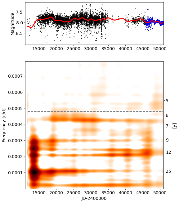
Figure 4: Long-term photometry and time-frequency analysis of V815 Her. Top: DASCH light curve of $\approx$100 years for V815 Her from scanned photographic plates (black dots) supplemented with photoelectric data (blue dots) spanning more than a century between 1890-1998 with 5 years’ overlap. The spline smoothed data are indicated by a red line. Bottom: Time-frequency analysis for the available photographic+photoelectric data of V815 Her using the TiFrAn code (Kolláth & Oláh 2009). The plot indicates dominant cycles of different lengths and amplitudes on timescales corresponding to $\sim$6.5, $\sim$9.1, $\sim$11.5, $\sim$13 and $\sim$26 years, the latter two are probably multiples of the 6.5-year period. Dashed lines indicate the 2092 d period of the wide orbit and its double at 4184 d ($\approx$11.5yr). See the text for more.

3 Spectroscopic data and astrophysical properties of V815 Her Aa

3.1 STELLA-SES spectra

The spectroscopic observations were carried out with the 1.2-m STELLA-II telescope of the STELLA robotic observatory (Strassmeier et al. 2010) located at Izaña Observatory in Tenerife, Spain. STELLA-II is equipped with the fibre-fed, fixed-format STELLA Echelle Spectrograph (SES) providing an average spectral resolution of $R=55,000$ along the covered 3900–8800 Å wavelength range. Further details on the performance of the system and the data-reduction procedure can be found in Weber et al. (2008, 2012).

Altogether 621 high-resolution spectra were recorded between 07 March and 11 November, 2018. With a default exposure time of 3000 s an average signal-to-noise ratio (S/N) of $\approx$200:1 could be reached and only 18 spectra had to be discarded due to their poor quality. This data set were used for both the spectral synthesis detailed in the next section and the Doppler-inversions (see Sect. 4). The observing log is summarized in Table B. Assuming synchronized rotation for the G star in the close binary subsystem V815 Her A, the rotational phases are calculated using the orbital period from Fekel et al. (2005) according to the following equation:

$$\mathrm{HJD}=2450204.5802+1.80983433\times E.$$ (2)

The zero phase is the time of maximum radial velocity, i.e., the primary component is closest to us in $\phi$=0.75 phase, accordingly, the $\lambda$=270^∘ longitude of the primary is facing the secondary.

3.2 Spectral synthesis

For the determination of some of the basic astrophysical parameters, we used the spectral synthesis code SME (Piskunov & Valenti 2017). Ten good quality (S/N$\sim$200) STELLA-SES echelle spectra were randomly selected to carry out spectral synthesis independently on each. During the computations, local thermodynamical equilibrium (LTE) was assumed and MARCS atmospheric models (Gustafsson et al. 2008) were used. Atomic line data were taken from the VALD line database (Kupka et al. 1999). A global macroturbulence relationship was adopted from Valenti & Fischer (2005, see their Eq. 1). The parameters, $T_{\rm eff}$ effective temperature, $\log g$ surface gravity, $[\mathrm{Fe}/\mathrm{H}]$ metallicity, and $v_{\rm mic}$ microturbulence were determined iteratively; for details on the fitting method see Kriskovics et al. (2019). For the fits the equatorial rotational velocity $v\sin i$ was kept at 30 kms^-1 since the Doppler-inversion (see Sect. 4 in this paper) proved to be artifact-free at this value, while using e.g. 27 kms^-1 and 33 kms^-1 caused severely artifact-ridden results having unrealistic equatorial brightening with polar darkening or polar brightening with equatorial darkening, respectively. We note that if $v\sin i$ was treated as a free parameter as well, the process yielded only slightly different results compared to the value of 30 kms^-1.

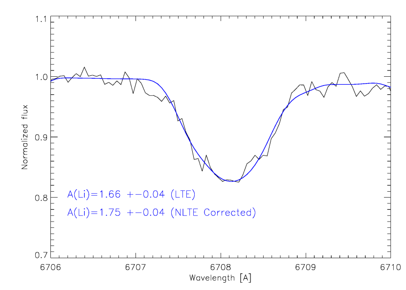
Figure 5: An example plot of the observed Li i 6707 Å spectral region (black) fitted with a synthetic spectrum (blue).

Lithium 6707Å abundance was determined also by SME using LTE synthesis together with 3D-NLTE departure coefficients taken from Harutyunyan et al. (2018). We selected the same ten spectra of high signal-to-noise ratio as above, for which we determined the lithium abundance separately. Averaging these yielded logarithmic abundances of $A(\mathrm{Li})_{\mathrm{LTE}}=1.66\pm 0.04$ and $A(\mathrm{Li})_{\mathrm{NLTE}}=1.75\pm 0.04$. Here, logarithmic abundance is defined as $A(\mathrm{Li})=\log(N_{\mathrm{Li}}/N_{\mathrm{H}})+12$ where $N_{\mathrm{Li}}$ and $N_{\mathrm{H}}$ are the number densities of lithium and hydrogen, respectively. Fig. 5 shows an example fit to the observed Li i 6707 Å spectral region. In a solar-like star like the G component in the V815 Her system, Li-6707 is gradually depleting during the pre-MS evolution over a few tens of Myr (e.g. Hillenbrand 2009). According to Somers & Pinsonneault (2015), in the Pleiades, $A(\mathrm{Li})$ typically decreases from the initial 3.3 to below $\sim$1.0 by the age of $\sim$100 Myr, however, highly dependent on the evolutionary models applied. Nevertheless, the correspondingly estimated age of a few tens of Myr is also consistent with the result of our spectral energy distribution analysis; see Sect. 3.3.

Table 3: Adopted/calculated astrophysical parameters for V815 Her Aa

Parameter	Value
Spectral type	G6 V
Gaia distance [pc]	$32.087\pm 0.127$
$V_{\rm br}$ [mag]	7.56
$(B-V)$ [mag]	0.71
$M_{\rm bol}$ [mag]	$4.90\pm 0.03$
Luminosity [${L_{\odot}}$]	$0.87\pm 0.03$
$T_{\rm eff}$ [K]	5582$\pm$63
$\log g$ (in cgs)	4.27$\pm$0.04
$v\sin i$ [ kms-1]	$30.0\pm 1.5$
$P_{\rm rot}=P_{\rm orb}$ [d]	$1.80983433$
Inclination of the rotation axis [°]	$75\pm 5$
Radius [$R_{\odot}$]	$1.1\pm 0.1$
Mass [$M_{\odot}$]	$\lesssim$1.0
Microturbulence [ kms-1]	$1.14\pm 0.19$
Macroturbulence [ kms-1]	4.2
Metallicity [Fe/H]	0.06$\pm$ 0.03
$A(\mathrm{Li})_{\mathrm{LTE}}$ (log)	1.66$\pm$0.04
$A(\mathrm{Li})_{\mathrm{NLTE}}$ (log)	1.75$\pm$0.04
Age [Myr]	$\approx$30

3.3 Analysis with VOSA

We performed a spectral energy distribution (SED) synthesis using the virtual observatory (VO) SED analyzer tool VOSA (Bayo et al. 2008) to build the SED of V815 Her from the available VO catalogues and surveys (GALEX, Tycho, SLOAN/SDSS, Pan-Starrs, Gaia, 2MASS, AKARI/IRC, WISE, and IRAS). For fitting the resulting SED in Fig. 6 ATLAS9 Kurucz ODFNEW/NOVER models (Castelli & Kurucz 2003) were used with the nearest grid values of $T_{\rm eff}$=5500 K effective temperature, $\log g$=4.5 surface gravity, and $[\mathrm{Fe}/\mathrm{H}]$=0.2 metallicity.

It is noteworthy that the SED (see Fig. 6) shows an excess towards infrared (IR) wavelengths. This could be the characteristics of a very young age since pre-main sequence stars of $\lesssim$10 Myr (Williams & Cieza 2011) usually possess primordial protoplanetary disc, which causes excess in near-IR (cf. Sect. 3.2).

In Fig. 7 we plotted the star on the Hertzsprung$-$Russell-diagram (HRD) along with theoretical isochrones and evolutionary tracks for the most suitable Geneva model (Haemmerlé et al. 2019). According to the plot, the age of the G star with $M/M_{\odot}\lesssim 1.0$ mass ratio is $\approx$26 million years. We note, however, that errors of age determination increase towards the zero-age main sequence (ZAMS) as the isochrones line up more and more densely. Nevertheless, this age determination is in agreement with the measured Li-6707 abundance in Fig. 5.

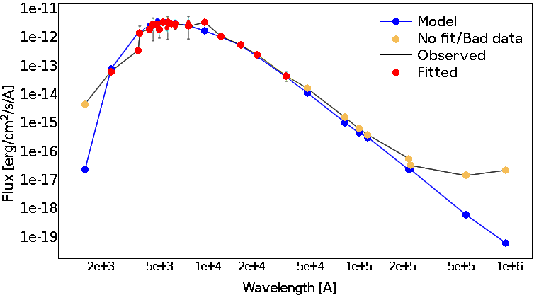
Figure 6: Spectral energy distribution for V815 Her generated by the VOSA SED analyzer tool (Bayo et al. 2008). The synthetic spectrum (blue line) is fitted to the archival photometry (red dots) from the available VO catalogues and surveys using ATLAS9 Kurucz ODFNEW/NOVER models with $T_{\rm eff}$=5500 K effective temperature, $\log g$=4.5 surface gravity, and [Fe/H]=0.2 metallicity.

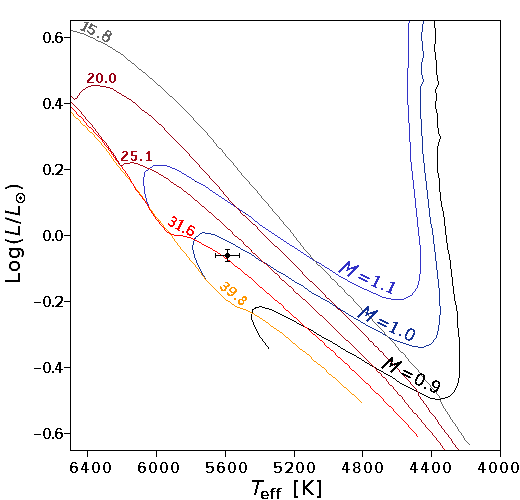
Figure 7: Position of V815 Her Aa (black dot) on the HRD plotted by using the VOSA SED analyzer tool (Bayo et al. 2008). Evolutionary tracks for the Geneva model (Haemmerlé et al. 2019) indicate an age of 30 Myr for a $M$$\lesssim 1$$M_{\odot}$ ZAMS star.

Table 4: Temporal distribution of the subsequent data sets for each individual Doppler image.

Data	Mean-HJD	Mean-date	Number	Data range	Data range
subset	2 450 000+	yyyy-mm-dd	of spectra	in days	in $P_{\rm rot}$
S01	8202.0111	2018-03-24	12	6.069	3.354
S02	8212.6014	2018-04-04	15	8.094	4.472
S03	8223.9904	2018-04-15	17	8.100	4.475
S04	8238.1401	2018-04-29	29	8.161	4.509
S05	8248.3858	2018-05-09	33	8.147	4.502
S06	8255.8846	2018-05-17	27	6.175	3.412
S07	8263.4391	2018-05-24	30	8.175	4.517
S08	8272.1472	2018-06-02	38	7.234	3.997
S09	8280.1488	2018-06-10	31	8.168	4.513
S10	8289.2001	2018-06-19	47	7.255	4.009
S11	8296.4747	2018-06-26	39	6.219	3.436
S12	8303.9658	2018-07-04	38	7.204	3.981
S13	8315.0355	2018-07-15	29	6.124	3.384
S14	8324.4312	2018-07-24	31	6.220	3.437
S15	8357.6721	2018-08-27	38	8.128	4.491
S16	8367.9366	2018-09-06	35	10.001	5.526
S17	8381.8476	2018-09-20	28	8.075	4.462
S18	8390.1971	2018-09-28	18	7.115	3.931
S19	8402.4761	2018-10-10	10	6.015	3.323

3.4 Luminosity and size

The Gaia EDR3 parallax of $\pi=31.1649\pm 0.1225\,\mathrm{mas}$ (Gaia Collaboration et al. 2016, 2021) yields a distance of $d=32.087\pm 0.127\,\mathrm{pc}$ for V815 Her. Assuming $V_{\rm br}\approx 7\aas@@fstack{m}56$ for the brightest $V$ magnitude with $B-V$ of 0$\aas@@fstack{m}$71 (cf. Fekel et al. 2005), and neglecting interstellar extinction yields an absolute visual magnitude of $M_{V}=5\aas@@fstack{m}03\pm 0\aas@@fstack{m}03$. Taking the $BC=-0.132$ bolometric correction from Flower (1996) gives a bolometric magnitude of $M_{\mathrm{bol}}=4\aas@@fstack{m}90\pm 0\aas@@fstack{m}03$. This gives $L/L_{\odot}=0.87\pm 0.03$ when using a value of $M_{\mathrm{bol},\odot}=4\aas@@fstack{m}74$ for the Sun.

Assuming an inclination of $i$=75$\pm 5^{\circ}$ (cf. Fekel et al. 2005), the projected equatorial rotational velocity $v\sin i$ of 30 kms^-1 with $\pm$1.5 kms^-1 error (see Sect. 3.2) would yield a stellar radius of $R/R_{\odot}=1.1\pm 0.1$. We note, that at a distance of $\approx$32 pc the estimated limb-darkened angular diameter of the G star of 0.346($\pm$0.009) mas (Mid-infrared stellar Diameters and Fluxes compilation Catalogue V10, Cruzalebes et al. 2019) would yield a similar radius of $\approx$1.2$R_{\odot}$. Although the $\gtrsim$1.1$R_{\odot}$ size is a bit larger than predicted for a non-magnetic G5 ZAMS star, still, such inflation is indeed to be expected for a ZAMS star with enhanced surface magnetic activity (cf. Jackson et al. 2016, and their references). When combining this radius with the effective temperature, the Stefan$-$Boltzmann law would give $L/L_{\odot}$ ratio of 1.05$\pm$0.15, still in line with the value derived from the bolometric magnitude, if the estimated errors are taken into account. Moreover, the 1.1$R_{\odot}$ radius, when combined with the most likely mass ratio of $M/M_{\odot}\lesssim 1.0$ (cf. Fig. 7 and Fekel et al. (2005)) would yield $\log g\approx 4.31$ for the G component in a pretty good agreement with the one obtained from SME.

In Table 3 we summarize the astrophysical parameters of the G star determined in our study, along with the others adopted from the literature.

4 Surface temperature maps of the G star

4.1 Imaging code iMAP

To reconstruct the surface temperature maps we use the state-of-the-art Doppler imaging code iMAP (Carroll et al. 2012). This code carries out multi-line inversion on a list of photospheric lines. We selected 38 non-blended absorption lines from the 5049-6750 Å region with suitable line-depth, temperature sensitivity and well-defined continuum. The stellar surface is modeled on a 5${}^{\circ}\times$5^∘ spherical grid. Each local line profile is computed with a full radiative solver (Carroll et al. 2008). The local line profiles are disk integrated, and the individually modeled disk-integrated lines are averaged. Atomic line data are taken from the Vienna Atomic Line Database (VALD, Kupka et al. 1999). Model atmospheres from Castelli & Kurucz (2004) are interpolated for the necessary temperature, gravity, or metallicity values. When solving the radiative transfer, local thermodynamical equilibrium (LTE) is assumed. Additional input parameters are micro- and macroturbulence, and the projected equatorial velocity (see Sect. 3). For the surface temperature reconstructions iMAP uses an iterative regularization based on a Landweber algorithm (Carroll et al. 2012). The iterative regularization has been proven to always converge on the same image solution, therefore, no additional constraints are imposed (see Appendix A in Carroll et al. 2012).

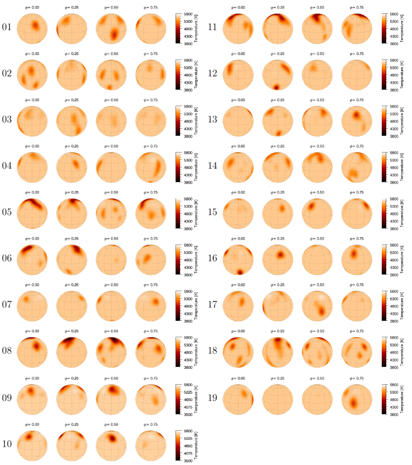
Figure 8: Nineteen time-series Doppler images of V815 Her for the 2018 observing season. From top to bottom, in chronological order, Doppler images S01-S10 are on the left, and Doppler images S11-S19 are on the right.

4.2 Time-series Doppler images

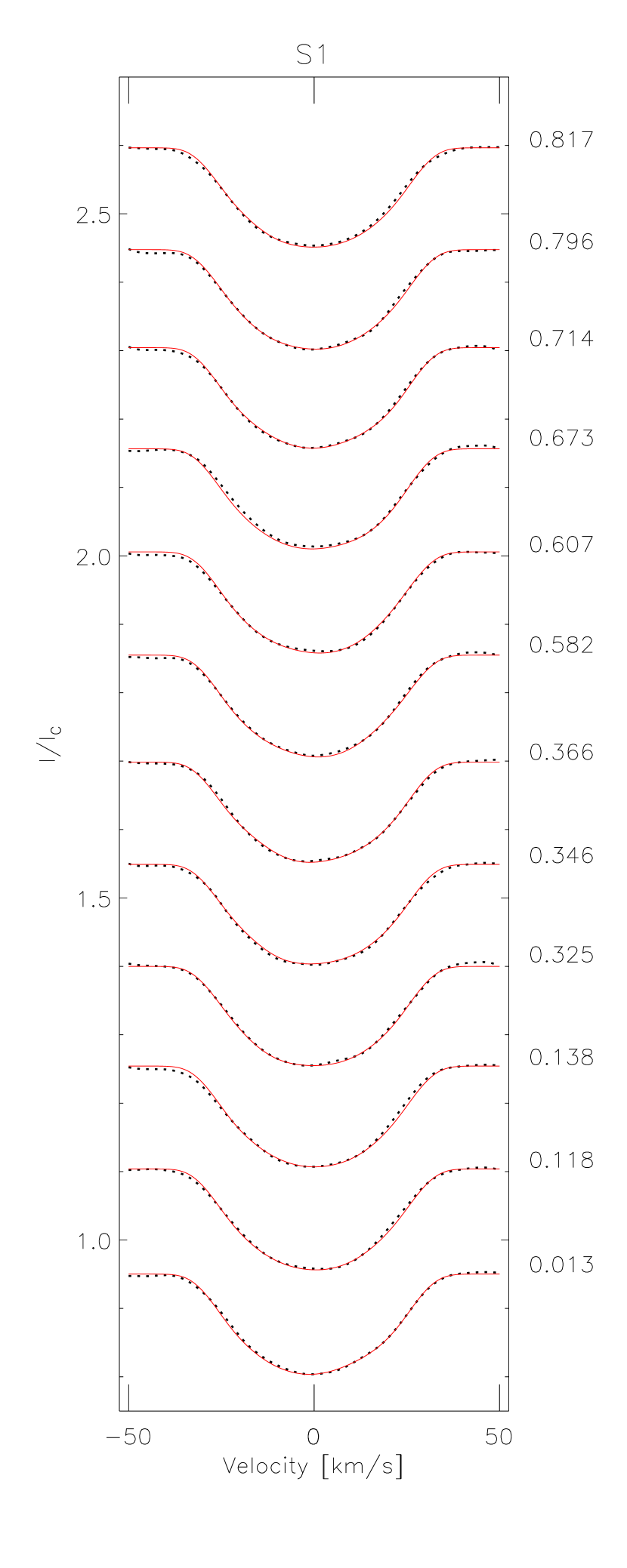
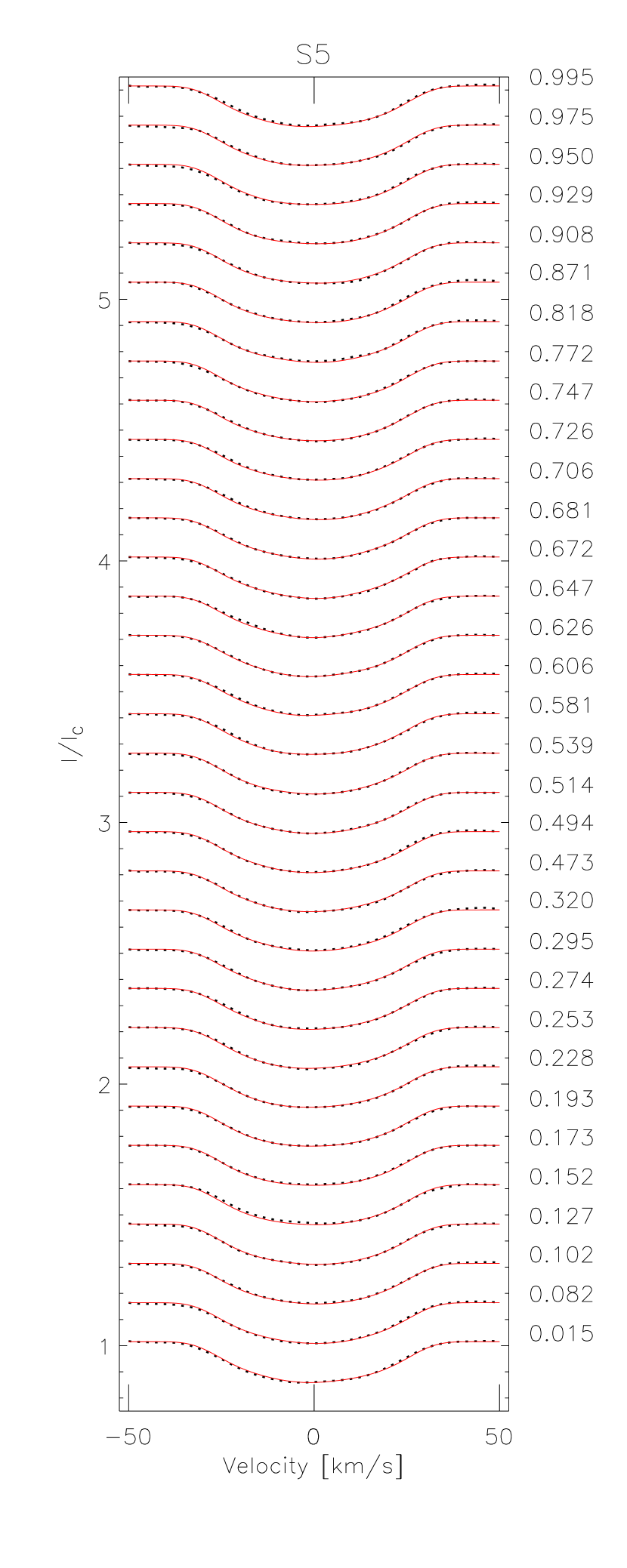
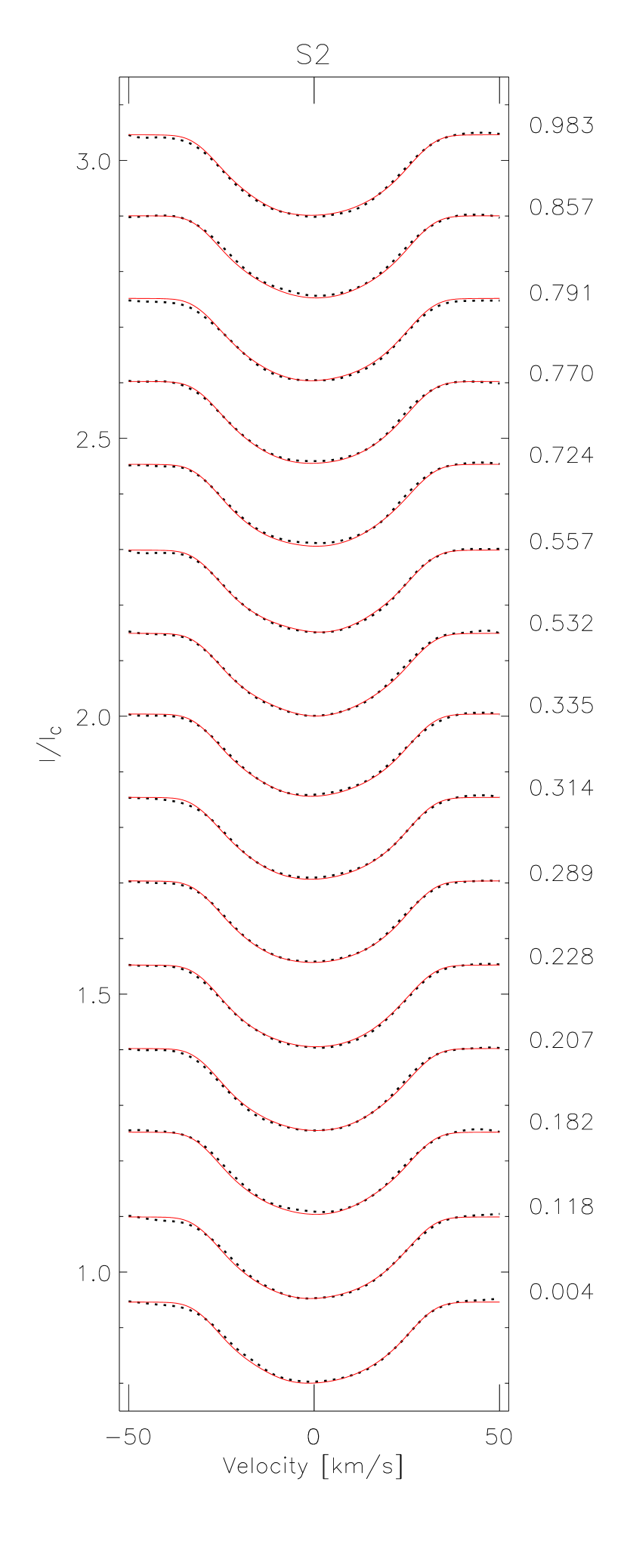
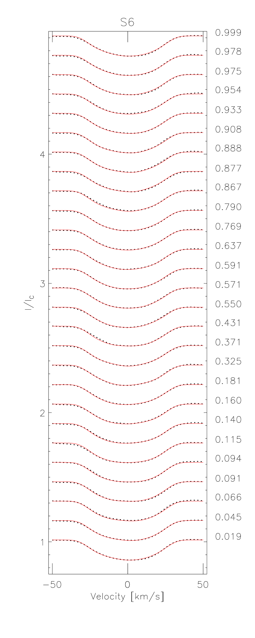
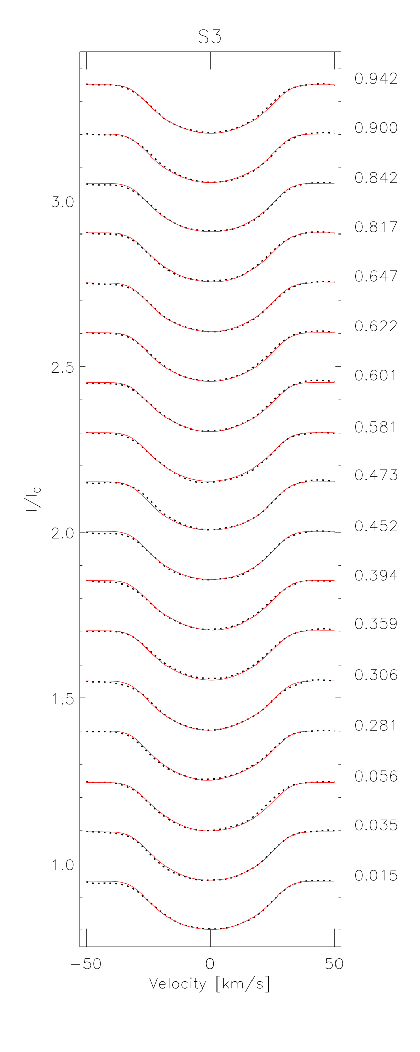
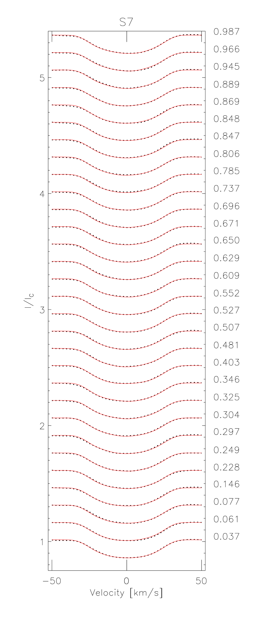
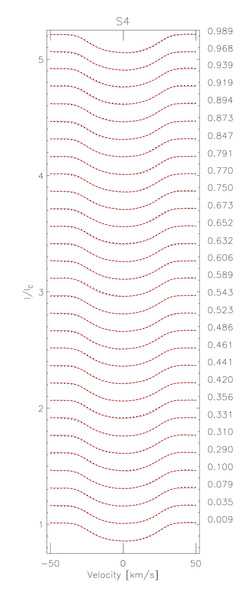
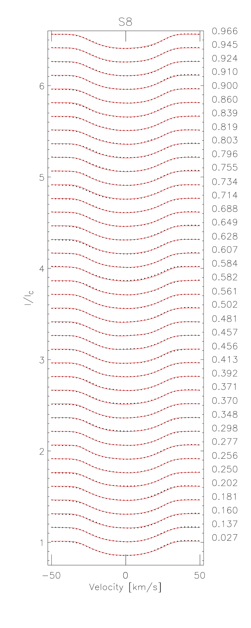
Figure 12: Fitted line profile subsets corresponding to the Doppler images S01-S08 presented in Fig. 8. The phase values of each profile are shown on the right side of the panels.

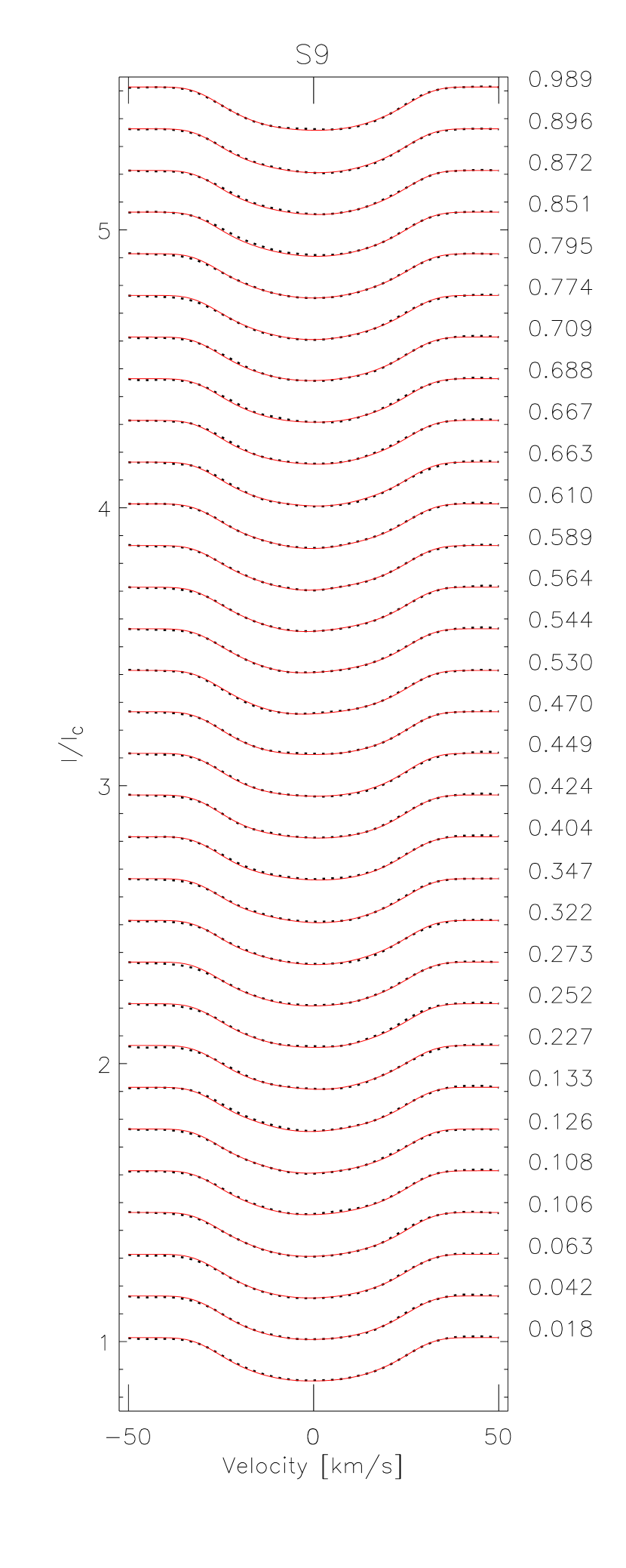
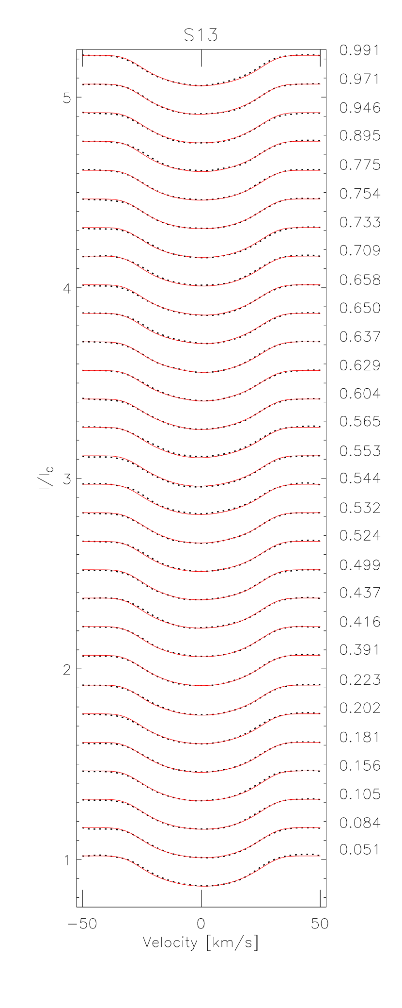
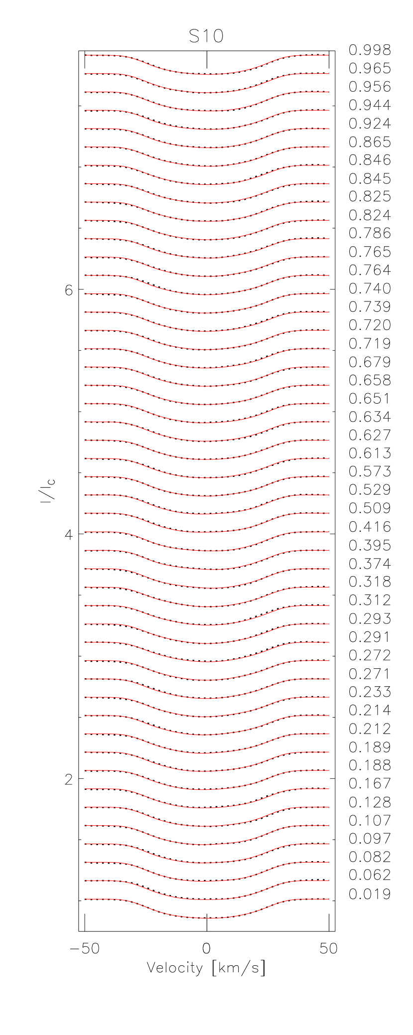
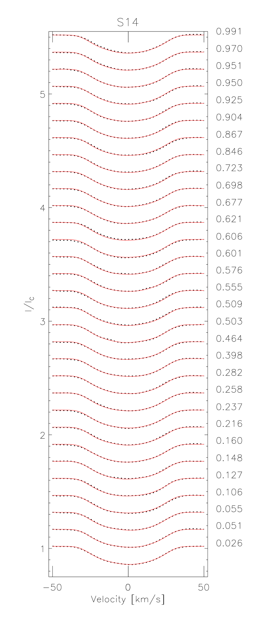
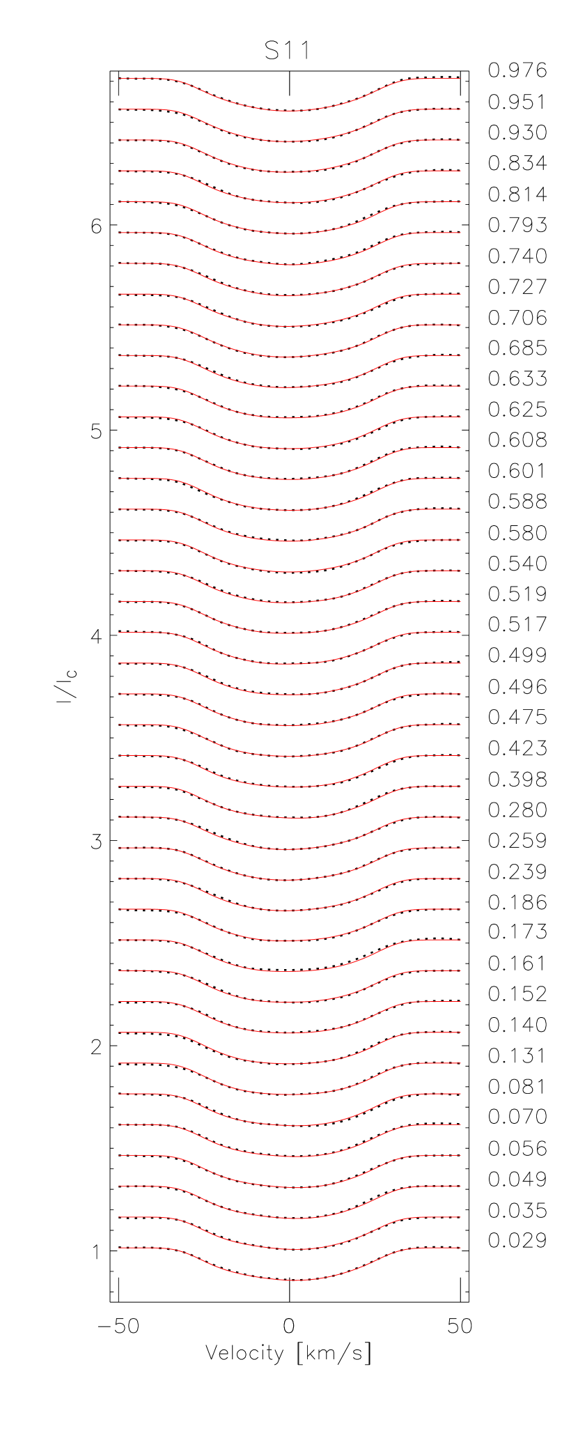
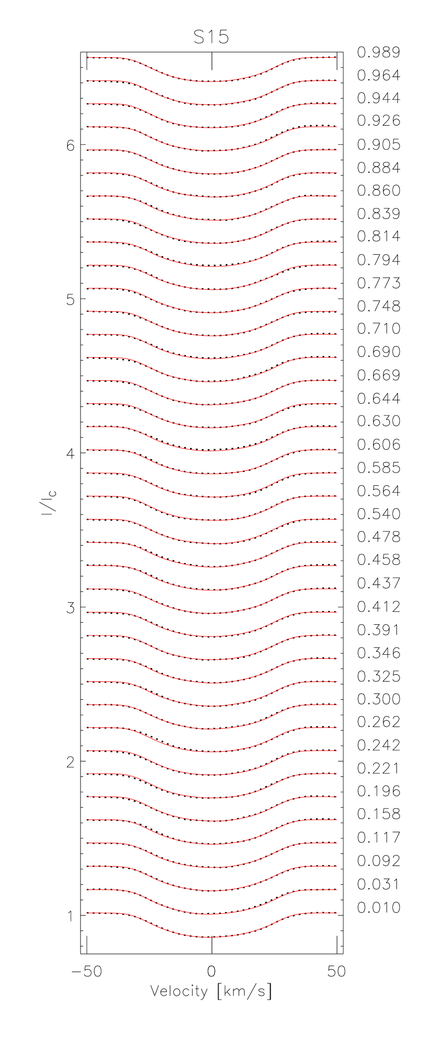
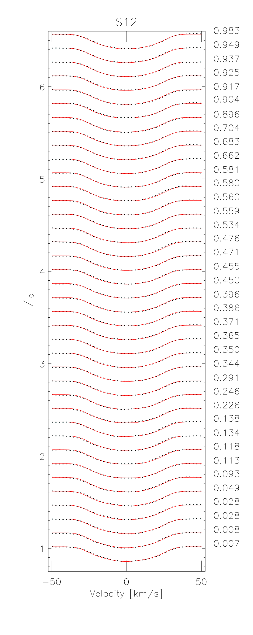
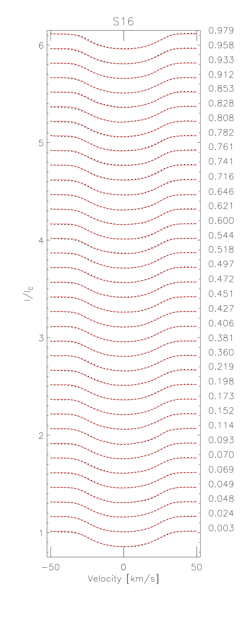
Figure 13: Fitted line profile subsets corresponding to the Doppler images S09-S16 presented in Fig. 8. The phase values of each profile are shown on the right side of the panels.

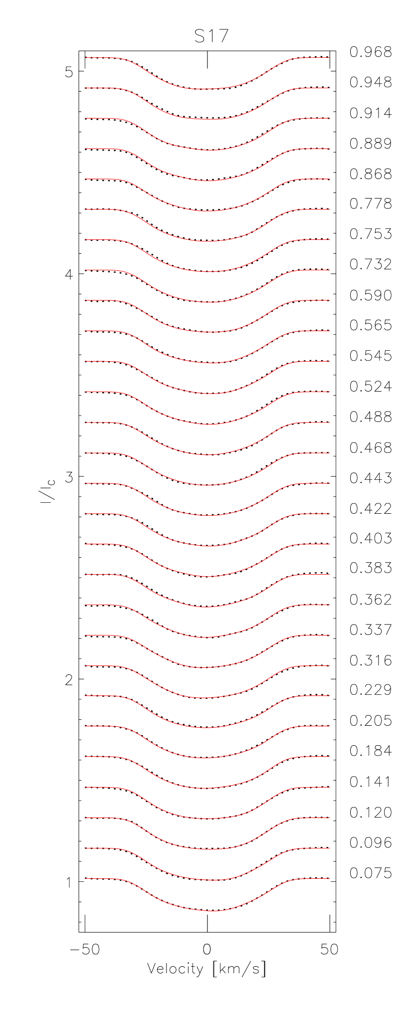
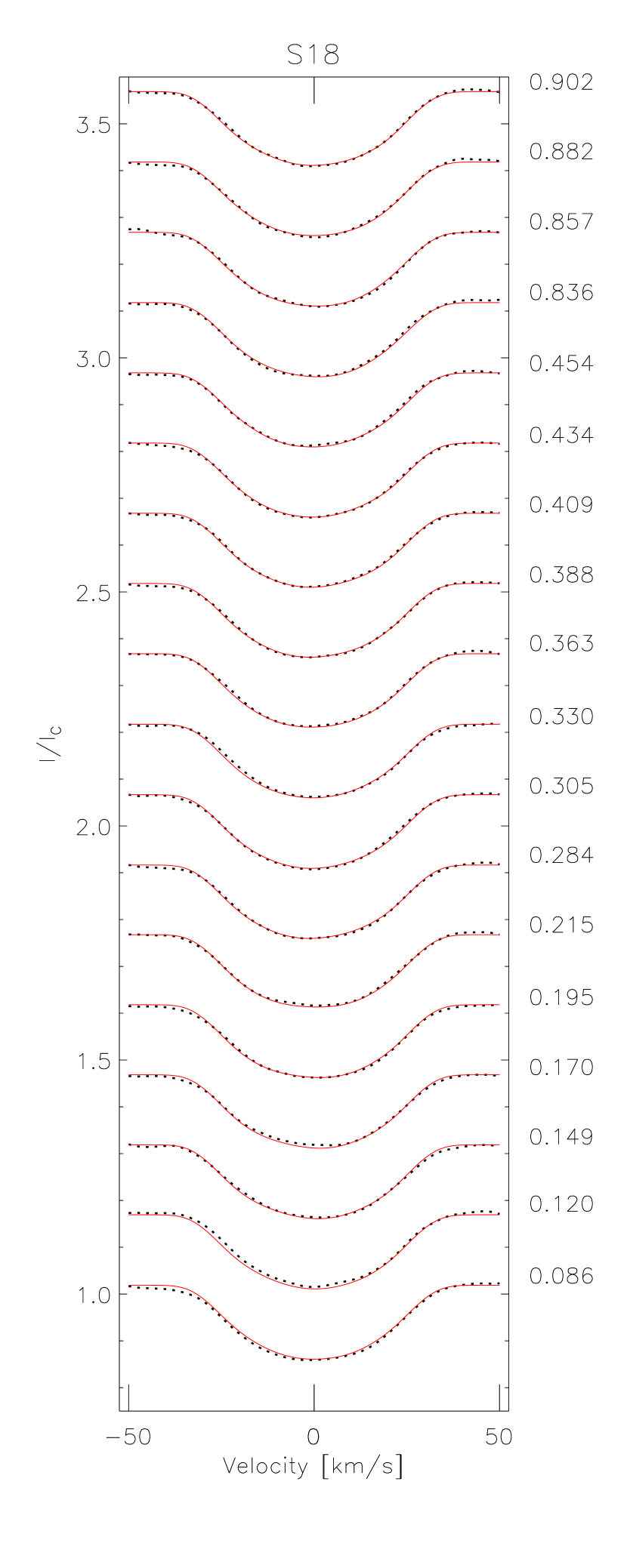
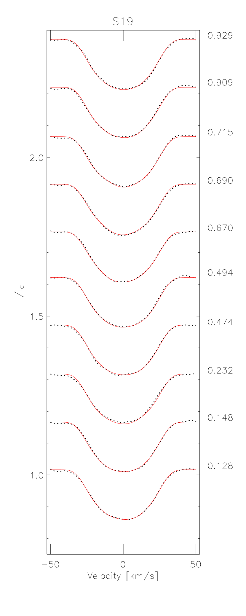
Figure 14: Fitted line profile subsets corresponding to the Doppler images S17-S19 presented in Fig. 8. The phase values of each profile are shown on the right side of the panels.

From the STELLA-SES spectra described in Sect. 3.1 we formed consecutive and independent data subsets in such a way that each of them covers the entire rotation phase in sufficient density. As a result, we created enough subsets for 19 time-series Doppler images. For the temporal distribution of the Doppler images see Table 4. The 19 time-series Doppler images of V815 Her Aa are plotted in Fig. 8, while the corresponding line-profile fits are given in Figs. 12-14 in Appendix C. In order to follow the change in the spot distribution even more spectacularly, in Appendix D, we also present our Doppler images in the Mercator projection. The surface temperature maps indicate a constantly changing surface structure on a time scale of a few weeks. Even the coverage of the visible pole with a spot is not continuous: in images S05-S06 and S08-S10 and in S18 we see strong polar spots, which, for example, are almost absent in images S03, in S07 and S19. Spot temperature ranges are not constant either, the highest contrast (see e.g., S08) reaches 1800 K, while the smallest temperature contrast (S07) is only a few hundred degrees. The lifespan of the longest-lived spots can typically be estimated at 2-3 weeks. However, with few exceptions, it is difficult to clearly point out the corresponding spots in successive images. The obvious main reason for this is rapid spot evolution, in which surface differential rotation is most likely involved. What is certain is that during the observed period we do not see a permanent polar spot, nor is there any sign of the formation of an active longitude. For further discussion of surface evolution see Sect. 5.4.

4.3 Surface differential rotation

The latitude dependent surface rotation can usually be inferred from the cross-correlation of two successive Doppler images (Donati & Collier Cameron 1997). However, random changes in spot distribution can easily mask the expected cross-correlation pattern of differential rotation. Therefore, for the detection of the surface shear operating in the background, we use ACCORD (e.g., Kővári et al. 2012, 2015), a technique which enables the averaging of latitudinal cross-correlations in the case of a sufficient number of pairs of Doppler images not too distant in time, this way suppressing the effect of randomness and amplifying the correlation pattern attributed to surface differential rotation.

The overall correlation pattern in the resulting average cross-correlation map (Fig. 9) is fitted by a rotational law in the form

$$\Omega(\beta)=\Omega_{\mathrm{eq}}-\Delta\Omega\sin^{2}\beta,$$ (3)

where $\Omega(\beta)$ is the latitude ($\beta$) dependent angular velocity, while $\Omega_{\mathrm{eq}}$ is the angular velocity at the equator, and $\Delta\Omega=\Omega_{\mathrm{eq}}-\Omega_{\mathrm{pole}}$ gives the difference between the equatorial and polar angular velocities. The dimensionless surface shear parameter $\alpha$ is defined as $\alpha_{\mathrm{DR}}=\Delta\Omega/\Omega_{\mathrm{eq}}$. The resulting fit indicates a weak solar-type differential rotation, with $\Omega_{\mathrm{eq}}=199.06\pm 0.40$°/day and $\Delta\Omega=1.99\pm 0.60$°/day, yielding $\alpha_{\mathrm{DR}}=0.010\pm 0.003$ shear parameter. In comparison, the solar pole-to-equator angular velocity difference is $\Delta\Omega_{\odot}=4.1\degr$/day, i.e. twice that of V815 Her. In the average correlation map, the stronger correlations are observed at latitudes higher than $\approx$30°, this is probably due to the fact that at lower latitudes the spots have less contrast, and perhaps in connection with this, their lifetime is also shorter. According to the rotational law that best fits the average cross-correlation pattern, it is most likely that the equatorial regions of the G star are (most) synchronized to the orbit. We note that the errors of the fitted rotation law plotted in Fig. 9 were estimated based on the error bars of the locations with the best correlations at the different latitude bands. However, this is the error of the fitting process, which does not necessarily reflect the true errors resulting from the method.

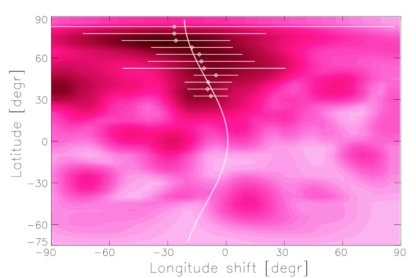
Figure 9: The average cross-correlation function map derived from 18 individual cross-correlations indicates how much longitude shift occurs at a given latitude due to surface shear during $\sim$6$P_{\rm rot}$ (which is the average time difference between the mean-HJDs of the consecutive maps; see Table 4).

5 Discussions

5.1 Multiplicity and dynamical evolution

The multiple nature of the V815 Her system makes it very special, as the size of the wide (i.e. AB, in other words ‘outer’ or ‘long’) orbit of the 2+2 hierarchical quadruple is relatively small, only $a_{\rm AB}$$\approx$1.6AU (cf. Table 2). The investigation of similar systems is also exciting because their secular gravitational evolution can have a significant impact on the future fate of the components. Long-term gravitational effects in such quadruple systems can have a serious impact on the evolution of the orbital eccentricities, since both binaries can act as a distant perturber on the other pair. Unfortunately, the evolution of such a 2+2 hierarchy is still an under-researched topic (but see Vokrouhlický 2016). It is certain, however, that this interaction is not only dynamic (e.g. Kozai oscillations, also known as von Zeipel-Lidov-Kozai mechanism or Lidov-Kozai cycles; for a recent review see Ito & Ohtsuka 2019), but due to the small size and large eccentricity of the wide orbit, as well as the compactness of the subsystems, tidal effects must also be taken into account (cf. Fabrycky & Tremaine 2007).

Due to the Kozai mechanism, in hierarchical triple systems a distant third body (as well as a distant close binary in a 2+2 system) may even decircularize the inner orbit (e.g. Hamers 2021, see also their references). The time scale of these Kozai cycles is in the order of $P^{2}_{\rm out}/P$, i.e. few times 10³ years. As a matter of fact, this can be seen in action on HD 74438 (Merle et al. 2022), a 2+2 hierarchical system in a highly eccentric wide orbit, where the eccentricity of one of the inner orbits was probably pumped by gravitational effects. According to this, the circularized close binaries of V815 Her will not necessarily remain so either. However, Kozai oscillations can be suppressed drastically when tidal friction enters the picture, shrinking and circularizing the inner orbit(s) on the tidal dissipation timescale (Fabrycky & Tremaine 2007). For both inner binaries, this timescale should be on the order of 10⁵ years (Van Eylen et al. 2016), i.e. much shorter than $\sim$10⁷-year age of the Aa component and so the assumed age of the four-star system (in case the components are coeval). For this reason, we do not expect a large-amplitude Kozai oscillation in the case of V815 Her.

We note that in Merle et al. (2022) HD 74438 is reported to be one of the shortest period 2+2 quadruple systems with $P\approx$5.7yr for the wide orbit, coincidentally almost exactly the same as the AB orbital period of V815 Her. Indeed, along with a few compact and coplanar (or even doubly eclipsing) 2+2 four-star system (Tokovinin 2018; Borkovits et al. 2021; Kostov et al. 2023; Zasche et al. 2023), V815 Her is among the shortest period 2+2 hierarhical systems. However, considering the size of the wide orbit, the V815 Her system is much more compact compared to HD 74438, which can be a significant difference in terms of the strength of secondary (i.e. tidal) effects; see also Sect. 5.3 below in this paper.

5.2 The V815 Her B close binary subsystem

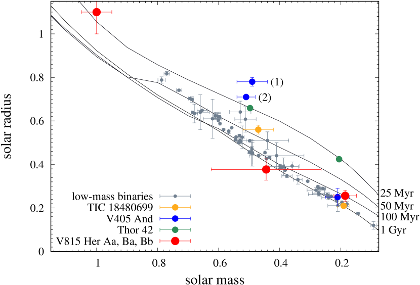
Figure 10: Mass-radius relation of low mass eclipsing binary stars with well-determined parameters from the compilation of Table B.2. from Schweitzer et al. (2019) plotted with grey dots. Coloured symbols (see legend) show the position of TIC 18480699 = 2MASS J04463285+1901432: Hebb et al. (2006), V405 And (1): Vida et al. (2009) and (2): Ribeiro et al. (2011), Thor 42 = CRTS J055255.7-004426: Murphy et al. (2020), and V815 Her Aa, Ba and Bb (present paper). Non-magnetic, solar metallicity isochrones are plotted from Baraffe et al. (2015).

The components of the low-mass eclipsing binary V815 Her B of the quadruple system are plotted on the mass-radius diagram on Fig.10 together with other eclipsing binary components from the literature. Note that the oversize of the primary of V405 And were determined by two different methods using independent data (cf. caption of Fig.10). In the figure the non-eclipsing component V815 Her Aa is also given for reference to the age determination. Together with V815 Her Ba+Bb three other systems are plotted in color (see the legends in Fig.10). While the masses of both the primaries and secondaries of these four systems are very similar to each other, laying on the two sides of the full-convection limit of $\approx$0.35 $M_{\odot}$ (Chabrier & Baraffe 1997), the primaries show about twofold difference in radius. The fully convective secondaries are quite similar to each other in size, except for Thor-42 (Murphy et al. 2020). This detailed study of Thor-42 was not able to simultaneously model the mass, radius, temperature and luminosity of the components.

The relative oversize of low-mass magnetically active stars compared to inactive stars is a known phenomenon (cf. Mullan & MacDonald 2001). Kraus et al. (2011) suggested rotation as a third parameter of the mass-radius relation. Fast rotation, maintained by the binarity influence the magnetic field and through this, the strength of the magnetic activity of the late-type dwarfs. MacDonald & Mullan (2021) modelled Thor-42 using both magnetoconvection and starspots and through this they were able to reconcile all stellar parameters of the system, but at a different age that Murphy et al. (2020) found. This result underlines the importance of magnetic field in estimating fundamental parameters of active stars. We may say that the apparent discrepancy between the ages of the components of the V815 Her quadruple system shown in Fig. 10 could be largely due to the magnetic activity of the components which, in the same time, could also be different star-by-star.

5.3 Brightness change along the wide orbit

In the top panel of Fig. 11 we plot the $V$ observations of V815 Her between 1984-98 from Jetsu et al. (2000). In these data we found a long-term brightness modulation, which showed an exciting coincidence with the approximate period of 5.73 yr of the outer (AB) orbit. Therefore, in the bottom panel of Fig. 11 we replot the $V$ data along with the folded light curve phased with the period of the wide orbit taken from Fekel et al. (2005). It is interesting that near zero phase (which is the periastron of the wide orbit), the brightness decreases, while away from it the brightness gradually increases. The question arises as to whether this is just a coincidence or really a change related to the wide orbit, and if it is the latter, then what is causing it.

On the other hand, the time-frequency analysis of the photometric data on a much longer term plotted in Fig. 4 does not show a strong cycle corresponding exactly to the period of the outer orbit, instead we see a strong signal of a 6.5-year cycle with gradually increasing period, and strangely, a signal that appears almost exactly at twice the orbital period. Nevertheless, it cannot be ruled out that the slowly changing, roughly 6.5-year photometric period is the changing activity cycle of the Aa component, which is perhaps triggered along the wide orbit. According to Fekel et al. (2005) the eccentricity of the wide orbit is quite large ($\approx$0.77), therefore gravitational effects exerted on the G star by V815 Her B change significantly along the outer orbit. Tidal interactions have indeed a potential impact on the internal structure and the turbulent/mixing processes (e.g. Toledano et al. 2007; Koenigsberger et al. 2021), ultimately, therefore, for the operation of the magnetic dynamo. This may also result in a change of the strength of spot activity of the G star, which ultimately causes the long-term change in brightness. We note here that such a possible binary-induced, i.e. tidally triggered activity was reported in Strassmeier et al. (2011).

An alternative explanation could be that the brightness change along the wide orbit is somehow related to the dust-gas material component of any kind (circumstellar or circumbinary) present in the quadruple star system. Assuming that there is a circumbinary disk around the Ba+Bb binary (consistently with the infrared surplus indicated by Fig. 6), such a disc if tilted to the plane of the wide orbit, can reflect the radiation of the G star differently, depending on their mutual position, i.e. the orbital phase. In our case, the reflected light can only be estimated cautiously in the case of a disc of unknown composition, size and geometry. However, if we estimate the contribution of the reflection from the disc to $\lesssim$1% (which is a rough upper estimate, cf. Bromley et al. 2021), then we can only explain a few percent of the long-term change in the mean brightness with reflection (say, $\lesssim$0.02 mag). Therefore, we conclude that changing spot activity results in the modulated brightness along the outer orbit, even though light reflected from any disc contributes little, if at all.

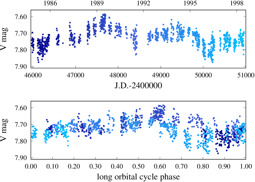
Figure 11: Top: $V$ light curve of V815 Her from Jetsu et al. (2000) between 1984-98. Bottom: Folded light curve using the 5.73 yr (=2092.2 d) period of the wide orbit. As zero phase the time of the periastron passage was set. The continuous color gradient helps to distinguish successive phases.

5.4 Surface evolution of V815 Her Aa

5.4.1 Spot decay and turbulent-driven magnetic diffusion

According to observations, the lifetime of sunspots depends on their area, based on which linear and nonlinear spot decay theories were born (e.g., Bumba 1963; Krause & Ruediger 1975; Petrovay & van Driel-Gesztelyi 1997; Hathaway & Choudhary 2008; Litvinenko & Wheatland 2015; Muraközy 2021; Forgács-Dajka et al. 2021, etc.). The underlying theories assume different mechanisms that also depend on the morphology of the sunspots/sunspot groups. When starspot lifetimes and starspot decay are discussed based on the solar analogy, the question arises as to whether it is a matter of scaling or other considerations are necessary (see e.g., Namekata et al. 2019, and their references). The average spot area on V815 Her is about a factor of $\sim$100 larger compared to long-lived big sunspots (see Fig. 8). We note however, that the spatial resolution of our Doppler images does not reach the size range of sunspots, but in principle they are able to resolve surface structures corresponding to the largest sunspot groups. In this context, it is perhaps more reasonable to compare the starspots of our Doppler images with groups of sunspots instead of large individual sunspots.

As for the spot lifetime, based on our time-series Doppler images, the spotted surface of V815 Her is completely rearranged in a few steps, typically within $\sim$25-50 days (cf. Fig. 8 and Table 4). This is therefore the approximate upper limit of spot lifetime. At the same time, the lifespan of individual spots can vary widely. The shortest-lived spots can only be observed in one or at most two consecutive images, so their lifetime is $\sim$10-15 days.

We emphasize here, that it is difficult to discuss on the starspot decay in the context of sunspot theory without knowledge of the true morphology of starspots, i.e., do we see monolithic spots on Doppler images or clusters of smaller spots? It is even possible that one does not exclude the other, nevertheless, usually the limited spatial resolution of observations does not allow us to make a clear distinction (but see Järvinen et al. 2018). Moreover, spot decay may strongly be influenced by surface and subsurface flows.

Işik et al. (2007) modeled the temporal decay of the surface magnetic flux when assuming different spot configurations while large-scale flows (differential rotation, meridional circulation) are switched on and off. Their results indicate that spot conglomerates decay faster compared to large monolithic spots, and flows also play an important role in speeding up the decay. We note that the $\Delta\Omega\approx 2^{\circ}$/d surface shear on V815 Her is much weaker than on the Sun (see Sect. 4.3). If we take into account the $t_{\rm l}$ lap time, i.e. the time taken for the equator to lap the poles, then in the case of V815 Her we get $360^{\circ}/\Delta\Omega$=180 d (i.e. about twice the solar lap time of $\sim$88 d). This is much longer than the observed spot lifetimes on V815 Her, therefore, differential rotation is likely to play a minor role (if at all) in spot decay. However, even with flows, the simulations in Işik et al. (2007) generally predict longer spot lifetimes than what we see on V815 Her.

Bradshaw & Hartigan (2014) argued that, assuming the same physical background and starting from the Gnevyshev$-$Waldmeier (hereafter GW) rule, the decay of sunspots and starspots can be scaled by the value of magnetic diffusivity through the turbulent scale length (which is connected to the supergranulation on the Sun). They suggested an anomalous turbulent-driven magnetic diffusion, which can account for the decay of either sunspots or starspots by scaling the characteristic supergranule/diffusion lengths.

By following the empirical GW rule, i.e. assuming a linear relationship between the maximum $A_{\rm s}$ spot area and its $t_{\rm s}$ lifetime, based on our time-series Doppler images, taking $t_{\rm s}$$\sim$20 d and $R_{\rm s}$$\sim$10^∘, equivalent of 1.3 10⁵ km, as average spot lifetime and corresponding characteristic maximum size, respectively, we can estimate a characteristic value of the spot decay rate $\Delta A_{\rm s}/\Delta t_{\rm s}$ of about $-$4.0 10⁴ km² s^-1. In Appendix F, we also present a more detailed study to measure the spot decay rate. Although the method is not mature enough yet, it is certainly more quantitative than the above estimate. We note that this detailed study yields even faster decay of about $-$7.0 10⁴ km² s^-1.

Now, using $t_{\rm s}$=20 d and $R_{\rm s}$=1.3 10⁵ km (see above), we get from $t_{\rm s}\sim R_{\rm s}^{2}/\eta_{\rm T}$ (Bradshaw & Hartigan 2014, their Eq. 3) a value of $\eta_{\rm T}\approx 10^{4}$ km² s^-1 for the turbulent diffusivity. According to Chae et al. (2008, their Eq. 19), from

$$\eta_{\rm T}=\bigg{(}\frac{l}{260\,{\rm km}}\bigg{)}^{5/4}$$ (4)

this value would yield a turbulent scale length of $l$=4.2 10⁵ km or $\approx$0.55 $R_{*}$, i.e., in the order of the stellar radius. Indeed, if we assumed an even faster spot decay from Appendix F, we would get about twice this amount. This large turbulent scale length is probably an overestimate, which may result from an overestimation of the maximum spot size. However, if, for example, several smaller spots were assumed instead of a monolithic spot, the turbulent scale length could also be reduced to a more plausible value (cf. Bradshaw & Hartigan 2014). Finally, we should also note that our measurement of the spot decay rate can be significantly distorted if, in addition to the spot shrinking, a rapid flux emergence occurs simultaneously in the same region. This would limit the validity of the interpretation that the observed spot decay rate and turbulent diffusion are directly related.

5.4.2 Latitudinal and longitudinal distribution of spots

In order to make it easier to assess the distribution of spots on the time-series Doppler maps, for each temperature reconstruction we calculated the sums of the $f$ filling factor values along the $\lambda$ longitude and $\beta$ latitude (we have 72 longitude and 36 latitude pixels on a 5${}^{\circ}\times$5^∘ spherical grid). When calculating $f_{\lambda}$ and $f_{\beta}$, we took into account the geometric distortion on the spherical surface according to the following formula:

$$f_{\lambda,\beta}=1-\frac{\sum_{i=1}^{n_{\lambda,\beta}}\cos(\beta_{i})T_{i}^{4}}{T_{\rm eff}^{4}\sum_{i=1}^{n_{\lambda,\beta}}\cos(\beta_{i})},$$ (5)

where $T_{i}$ and $\beta_{i}$ are the temperature and the latitude of the $i$th pixel, while the limit of the summation is the image pixel number over either the longitude ($n_{\lambda}$=72), or the latitude ($n_{\beta}$=33, since we do not see the star below $\beta$=$-$75^∘). The resulting spot filling factors for the nineteen Doppler images are shown in Appendix E. Based on the latitudinal distribution of the spots, we see that especially in the case of low spot coverage, the spots tend to appear at mid-latitudes. In these cases (e.g. S01-S02-S03-S04, S07, S12-S13, S18) a somewhat equatorially symmetric distribution is seen. On the other hand, at other times spots tend to appear at high latitudes, closer to the visible pole. We note however, that, since we cannot see the other pole and its immediate surroundings, we cannot say whether the appearance of the polar spots shows any symmetry to the equator.

Granzer et al. (2000) studied the dynamics of magnetic flux tubes in young stars by numerical simulations and found that at a rotation rate of V815 Her Aa the spot emergence latitude is most likely between 25^∘-50^∘ (see their ZAMS star model of 1 solar mass with $\sim$10$\Omega/\Omega_{\odot}$ rotation). However, similarly to V815 Her Aa, the coexistence of low-to-mid latitude spots and high latitude/polar spots on G-K type main sequence stars has already been supported by numerous Doppler imaging studies (e.g., Strassmeier 2009, and references therein). Moreover, EK Dra, the rapidly rotating young Sun, showed a very similar starspot distribution in the recent Doppler imaging study by Şenavcı et al. (2021), in which the polar and mid-latitude (¿20^∘) spots are also consistent with flux emergence and transport simulations. According to Granzer et al. (2000), after flux emergence at mid latitudes a poleward flux transport by meridional circulation and/or magnetic stresses could explain the formation of polar spots (for the formation of polar spots on rapid rotators see also Schrijver & Title 2001; Işık et al. 2018). Maybe a weak sign of this can be seen in some of our subsequent Doppler image pairs (S04-S05, S13-S14, S16-S17), where the formation of the polar spot is preceded by a nearby lower latitude spot, although the available time resolution is not enough for a strict conclusion. Here, we note that the internal structure of V815 Her Aa is indeed affected by its close companion Ab, and this may be important also from the point of view of magnetic flux tube dynamics (e.g., Schuessler et al. 1996; Holzwarth & Schüssler 2003a, b).

The longitudinal spot distribution, in contrast, is more random, we see no definite indication of the existence of active longitudes. Although the changes can still mostly be followed in successive images, however, no systematic pattern can be seen in the evolution of the spotted surface over the entire period.

5.4.3 Surface differential rotation

From our cross-correlation study, we infer that the active G star has a weak solar-type differential rotation. Actually, this finding is in a fair agreement with the recent results obtained for two similar close binary systems V471 Tau (Kővári et al. 2021) and EI Eri (Kriskovics et al. 2023) in which the active component preserves its rapid rotation as a result of synchronization, but at the same time the degree of surface shear due to differential rotation is presumably confined by tidal interaction. These observations support the idea that differential rotation is suppressed in low-mass stars tidally locked in close binary systems (see also Collier Cameron 2007, and their references). From a theoretical point of view, this kind of behavior is not unexpected, since a marked initial differential rotation structure would converge to rigid body-like rotation due to tidal shear energy dissipation (Koenigsberger et al. 2021). Our Fig. 9 also suggests that the equatorial region of V815 Her Aa is synchronized the most with the orbital period of V815 Her A. We note that this is consistent with tidal perturbations being expected to be strongest around equatorial latitudes.

6 Summary

The V815 Her system undoubtedly evolves dynamically and most likely magnetically, while the two subsystems, V815 Her A and B, interact gravitationally. Our main conclusions are summarized as follows:

• The wide component in V815 Her previously apostrophized as a ‘third body’ is actually an eclipsing close binary subsystem of two M dwarfs, i.e., V815 Her is a 2+2 hierarchical quadruple system.

• V815 Her is presumably a young system, supported by the infrared surplus indicated by the spectral energy distribution in Fig. 6. The young age is also supported by the lithium abundance that has not yet been depleted. In accordance with this, the evolutionary state of V815 Her Aa is a zero-age main sequence star, with an age of $\sim$30M years.

• A rapid spot evolution can be observed on the surface of the active G component V815 Her Aa, the spot distribution can change completely on a time range of few times ten days.

• We measured a weak solar-type surface differential rotation on the G star, which is probably suppressed by the tidal force of the close companion.

• Based on the long-term photometric data, we found a slowly increasing cycle length of about 6.5 years on average, which we interpret as a spot cycle. The length of the spot cycle is not necessarily closely related to the 5.73-year period of the wide orbit, but we would not rule out the possibility of this at this point. We suspect that the reason for the slow change may be the modulation due to the eccentricity of the wide orbit.

The case of V815 Her is a good example of the particular importance of tidal effects for the dynamo mechanism. For this reason, our quartet is certainly interesting for further study of how gravitational evolution of the system affects activity.

Appendix A Times of eclipsing minima from TESS light curves

Table 5: Times of minima of V815 Her B from Sector 26 (left), Sector 40 (middle), and Sector 53 (right) light curves.

BJD	Cycle	std. dev.	BJD	Cycle	std. dev.	BJD	Cycle	std. dev.
$-2\,400\,000$	no.	[d]	$-2\,400\,000$	no.	[d]	$-2\,400\,000$	no.	[d]
59010.396759	$-$1.0	0.005419	59390.969044	730.0	0.000579	59750.207340	1420.0	0.001752
59010.655434	$-$0.5	0.000611	59391.228904	730.5	0.001037	59750.467594	1420.5	0.001804
59010.917386	0.0	0.000308	59391.490881	731.0	0.000731	59750.729019	1421.0	0.000407
59011.177977	0.5	0.000852	59391.750806	731.5	0.000616	59750.986819	1421.5	0.000808
59011.436903	1.0	0.000463	59392.010439	732.0	0.000859	59751.249397	1422.0	0.000430
59011.703819	1.5	0.000760	59392.270268	732.5	0.000889	59751.509992	1422.5	0.002570
59011.958773	2.0	0.000525	59392.530909	733.0	0.000864	59751.770279	1423.0	0.000575
59012.216689	2.5	0.000328	59392.792132	733.5	0.000830	59752.028581	1423.5	0.001020
59012.478749	3.0	0.000290	59393.052663	734.0	0.000633	59752.287769	1424.0	0.007730
59012.730444	3.5	0.002701	59393.311377	734.5	0.001224	59752.550820	1424.5	0.002143
59012.997801	4.0	0.000545	59393.571995	735.0	0.000457	59752.810861	1425.0	0.000600
59013.256687	4.5	0.000690	59393.835471	735.5	0.002979	59753.071759	1425.5	0.001207
59013.523129	5.0	0.000308	59394.093038	736.0	0.000608	59753.330231	1426.0	0.002246
59013.781077	5.5	0.000576	59394.353760	736.5	0.000651	59753.593639	1426.5	0.001204
59014.041462	6.0	0.000656	59394.611848	737.0	0.000606	59753.853110	1427.0	0.000520
59014.298518	6.5	0.000725	59394.874266	737.5	0.001242	59754.112817	1427.5	0.002296
59014.558817	7.0	0.000488	59395.134036	738.0	0.000886	59754.372525	1428.0	0.000551
59014.822105	7.5	0.000913	59395.395363	738.5	0.000718	59754.633838	1428.5	0.002193
59015.089820	8.0	0.000879	59395.655174	739.0	0.001446	59754.893547	1429.0	0.001495
59015.345284	8.5	0.000737	59395.914606	739.5	0.000931	59755.155476	1429.5	0.003858
59015.602487	9.0	0.000425	59396.175866	740.0	0.000544	59755.414605	1430.0	0.002845
59015.866312	9.5	0.000881	59396.435910	740.5	0.001447	59755.675277	1430.5	0.001056
59016.127331	10.0	0.000456	59396.696363	741.0	0.000695	59755.934886	1431.0	0.000762
59016.381487	10.5	0.000440	59396.956394	741.5	0.007025	59763.483106	1445.5	0.002752
59016.643627	11.0	0.000205	59397.216360	742.0	0.000450	59763.746312	1446.0	0.000439
59016.907289	11.5	0.000494	59397.475688	742.5	0.029455	59764.004660	1446.5	0.001141
59017.165940	12.0	0.000268	59397.736504	743.0	0.000448	59764.264120	1447.0	0.000456
59017.421941	12.5	0.000440	59397.997957	743.5	0.018673	59764.523280	1447.5	0.001219
59017.685807	13.0	0.000299	59398.258231	744.0	0.000392	59764.785534	1448.0	0.000492
59017.949074	13.5	0.000974	59398.519739	744.5	0.000633	59765.045838	1448.5	0.001699
59018.206886	14.0	0.000320	59398.778495	745.0	0.000447	59765.306575	1449.0	0.000420
59018.467208	14.5	0.017412	59399.038859	745.5	0.002356	59765.566480	1449.5	0.002744
59018.724460	15.0	0.000314	59399.299451	746.0	0.000442	59765.827445	1450.0	0.001626
59018.984292	15.5	0.021397	59399.559764	746.5	0.001107	59766.087395	1450.5	0.001636
59019.246745	16.0	0.000258	59399.820430	747.0	0.000690	59766.347915	1451.0	0.000397
59019.507475	16.5	0.000424	59400.080220	747.5	0.000908	59766.608793	1451.5	0.001091
59019.765580	17.0	0.000468	59400.340231	748.0	0.000553	59766.868377	1452.0	0.000841
59020.025038	17.5	0.000752	59400.599451	748.5	0.002930	59767.128870	1452.5	0.004383
			59400.861610	749.0	0.000455	59767.388947	1453.0	0.000701
			59401.121024	749.5	0.006293	59767.648351	1453.5	0.008222
			59401.382010	750.0	0.000480	59767.907794	1454.0	0.000645
			59401.641153	750.5	0.001030	59768.170459	1454.5	0.005906
			59401.902890	751.0	0.000336	59768.429865	1455.0	0.000545
			59402.159590	751.5	0.008119
			59402.422958	752.0	0.000671
			59402.683010	752.5	0.009989
			59402.942458	753.0	0.001320
			59403.202713	753.5	0.000738
			59403.464449	754.0	0.000372
			59403.724330	754.5	0.000899
			59403.984932	755.0	0.000486
			59404.245716	755.5	0.001709

Appendix B Log of spectroscopic data

Table 6: Observing log of STELLA-SES spectra of V815 Her from 2018 used for the individual Doppler reconstructions shown in Fig. 8.

HJD	Date	Phase	S/N	Subset
8198.641	21.03.2018	0.011	197	S01
8199.672	22.03.2018	0.581	225	S01
8199.718	22.03.2018	0.607	221	S01
8200.641	23.03.2018	0.116	213	S01
8200.679	23.03.2018	0.138	228	S01
8201.646	24.03.2018	0.671	233	S01
8201.720	24.03.2018	0.712	211	S01
8203.679	26.03.2018	0.795	170	S01
8203.717	26.03.2018	0.817	171	S01
8204.636	27.03.2018	0.324	207	S01
8204.673	27.03.2018	0.344	209	S01
8204.711	27.03.2018	0.365	201	S01
8208.630	31.03.2018	0.530	213	S02
8208.676	31.03.2018	0.556	200	S02
8209.691	01.04.2018	0.117	178	S02
8211.617	03.04.2018	0.181	214	S02
8211.662	03.04.2018	0.205	218	S02
8211.700	03.04.2018	0.227	217	S02
8212.598	04.04.2018	0.723	211	S02
8212.681	04.04.2018	0.768	196	S02
8212.718	04.04.2018	0.790	179	S02
8213.620	05.04.2018	0.289	224	S02
8213.666	05.04.2018	0.312	218	S02
8213.703	05.04.2018	0.334	223	S02
8214.648	06.04.2018	0.856	223	S02
8216.687	08.04.2018	0.983	173	S02
8216.724	08.04.2018	0.002	189	S02
8219.577	11.04.2018	0.580	204	S03
8219.615	11.04.2018	0.599	216	S03
8219.652	11.04.2018	0.621	238	S03
8219.697	11.04.2018	0.645	225	S03
8222.655	14.04.2018	0.281	183	S03
8222.700	14.04.2018	0.304	207	S03
8223.624	15.04.2018	0.816	233	S03
8223.670	15.04.2018	0.842	225	S03
8224.606	16.04.2018	0.358	225	S03
8224.669	16.04.2018	0.392	227	S03
8225.586	17.04.2018	0.899	216	S03
8225.660	17.04.2018	0.940	230	S03
8226.584	18.04.2018	0.452	201	S03
8226.621	18.04.2018	0.471	225	S03
8227.602	19.04.2018	0.013	186	S03
8227.640	19.04.2018	0.035	177	S03
8227.677	19.04.2018	0.054	183	S03
8234.538	26.04.2018	0.846	199	S04
8234.586	26.04.2018	0.872	216	S04
8234.623	26.04.2018	0.892	212	S04
8234.668	26.04.2018	0.917	210	S04
8234.706	26.04.2018	0.939	190	S04
8235.575	27.04.2018	0.418	221	S04
8235.613	27.04.2018	0.440	218	S04
8235.650	27.04.2018	0.459	211	S04
8235.695	27.04.2018	0.485	212	S04
8236.567	28.04.2018	0.967	218	S04
8236.605	28.04.2018	0.988	216	S04
8236.642	28.04.2018	0.008	218	S04
8236.687	28.04.2018	0.034	223	S04
8237.571	29.04.2018	0.521	230	S04
8237.608	29.04.2018	0.543	227	S04
8237.692	29.04.2018	0.588	200	S04
8238.578	30.04.2018	0.078	196	S04
8238.615	30.04.2018	0.098	201	S04
8239.532	01.05.2018	0.605	209	S04
8239.578	01.05.2018	0.631	215	S04
8239.615	01.05.2018	0.650	221	S04
8239.653	01.05.2018	0.672	239	S04
8241.601	03.05.2018	0.749	208	S04
8241.639	03.05.2018	0.770	211	S04
8241.676	03.05.2018	0.790	223	S04
8242.579	04.05.2018	0.288	209	S04
8242.616	04.05.2018	0.310	199	S04
8242.654	04.05.2018	0.329	210	S04
8242.699	04.05.2018	0.355	168	S04
8243.535	05.05.2018	0.817	194	S05
8243.631	05.05.2018	0.871	195	S05
8245.508	06.05.2018	0.907	189	S05
8245.546	07.05.2018	0.929	213	S05
8245.583	07.05.2018	0.948	209	S05
8245.629	07.05.2018	0.974	210	S05
8245.666	07.05.2018	0.993	216	S05
8246.530	08.05.2018	0.473	214	S05
8246.567	08.05.2018	0.492	224	S05
8246.605	08.05.2018	0.514	233	S05
8246.650	08.05.2018	0.537	233	S05
8247.512	08.05.2018	0.014	214	S05
8247.632	09.05.2018	0.081	220	S05
8247.669	09.05.2018	0.101	202	S05
8248.535	10.05.2018	0.580	232	S05
8248.580	10.05.2018	0.604	228	S05
8248.617	10.05.2018	0.625	228	S05
8248.655	10.05.2018	0.646	246	S05
8248.700	10.05.2018	0.670	232	S05
8249.524	11.05.2018	0.126	232	S05
8249.569	11.05.2018	0.152	227	S05
8249.607	11.05.2018	0.171	229	S05
8249.644	11.05.2018	0.193	250	S05
8250.526	12.05.2018	0.681	227	S05
8250.571	12.05.2018	0.704	229	S05
8250.609	12.05.2018	0.726	222	S05
8250.646	12.05.2018	0.745	245	S05
8250.691	12.05.2018	0.771	232	S05
8251.516	12.05.2018	0.227	204	S05
8251.562	13.05.2018	0.252	201	S05
8251.599	13.05.2018	0.272	210	S05
8251.637	13.05.2018	0.293	219	S05
8251.682	13.05.2018	0.319	204	S05
8252.496	13.05.2018	0.768	223	S06
8252.533	14.05.2018	0.788	241	S06
8252.690	14.05.2018	0.876	233	S06
8253.502	14.05.2018	0.325	161	S06
8253.585	15.05.2018	0.371	172	S06
8253.694	15.05.2018	0.431	182	S06
8254.482	15.05.2018	0.865	209	S06
8254.520	15.05.2018	0.886	209	S06
8254.557	16.05.2018	0.908	215	S06
8254.603	16.05.2018	0.932	214	S06
8254.640	16.05.2018	0.953	206	S06
8254.678	16.05.2018	0.975	208	S06
8256.493	17.05.2018	0.976	221	S06
8256.531	18.05.2018	0.998	225	S06
8256.568	18.05.2018	0.017	225	S06
8256.614	18.05.2018	0.043	235	S06
8256.652	18.05.2018	0.065	214	S06
8256.697	18.05.2018	0.088	229	S06
8257.529	19.05.2018	0.548	226	S06
8257.566	19.05.2018	0.570	222	S06
8257.604	19.05.2018	0.591	235	S06
8257.687	19.05.2018	0.637	233	S06
8258.513	19.05.2018	0.092	182	S06
8258.551	20.05.2018	0.114	211	S06
8258.596	20.05.2018	0.140	215	S06
8258.633	20.05.2018	0.159	208	S06
8258.671	20.05.2018	0.181	232	S06
8259.482	20.05.2018	0.627	218	S07
8259.519	20.05.2018	0.649	226	S07
8259.557	21.05.2018	0.670	228	S07
8259.602	21.05.2018	0.694	228	S07
8259.677	21.05.2018	0.735	224	S07
8260.566	22.05.2018	0.228	215	S07
8260.604	22.05.2018	0.249	227	S07
8260.691	22.05.2018	0.296	211	S07
8261.573	23.05.2018	0.784	210	S07
8261.611	23.05.2018	0.804	224	S07
8261.686	23.05.2018	0.847	215	S07
8262.513	23.05.2018	0.302	225	S07
8262.551	24.05.2018	0.324	214	S07
8262.588	24.05.2018	0.346	224	S07
8262.691	24.05.2018	0.401	206	S07
8263.497	24.05.2018	0.846	237	S07
8263.535	25.05.2018	0.868	230	S07
8263.572	25.05.2018	0.887	226	S07
8265.483	26.05.2018	0.945	209	S07
8265.521	27.05.2018	0.964	232	S07
8265.558	27.05.2018	0.986	224	S07
8265.692	27.05.2018	0.059	215	S07
8266.453	27.05.2018	0.480	213	S07
8266.500	27.05.2018	0.506	213	S07
8266.537	28.05.2018	0.525	222	S07
8266.582	28.05.2018	0.551	240	S07
8266.685	28.05.2018	0.607	230	S07
8267.459	28.05.2018	0.037	212	S07
8267.531	29.05.2018	0.076	209	S07
8267.657	29.05.2018	0.145	215	S07
8268.450	29.05.2018	0.583	167	S08
8268.491	29.05.2018	0.607	201	S08
8268.529	30.05.2018	0.626	234	S08
8268.566	30.05.2018	0.648	211	S08
8269.451	30.05.2018	0.136	190	S08
8269.492	30.05.2018	0.159	217	S08
8269.530	31.05.2018	0.181	229	S08
8269.567	31.05.2018	0.200	219	S08
8269.654	31.05.2018	0.248	220	S08
8270.448	31.05.2018	0.688	215	S08
8270.494	31.05.2018	0.712	214	S08
8270.531	01.06.2018	0.733	204	S08
8270.569	01.06.2018	0.755	201	S08
8270.655	01.06.2018	0.802	183	S08
8271.476	01.06.2018	0.256	221	S08
8271.513	01.06.2018	0.275	220	S08
8271.550	02.06.2018	0.297	231	S08
8271.681	02.06.2018	0.368	222	S08
8272.452	02.06.2018	0.795	212	S08
8272.493	02.06.2018	0.817	216	S08
8272.530	03.06.2018	0.838	223	S08
8272.568	03.06.2018	0.858	236	S08
8272.658	03.06.2018	0.908	225	S08
8273.452	03.06.2018	0.348	223	S08
8273.494	03.06.2018	0.370	222	S08
8273.531	04.06.2018	0.391	219	S08
8273.568	04.06.2018	0.411	242	S08
8273.648	04.06.2018	0.456	223	S08
8274.450	04.06.2018	0.898	202	S08
8274.494	04.06.2018	0.922	222	S08
8274.532	05.06.2018	0.943	221	S08
8274.569	05.06.2018	0.965	232	S08
8274.680	05.06.2018	0.025	209	S08
8275.457	05.06.2018	0.455	239	S08
8275.502	05.06.2018	0.481	238	S08
8275.539	06.06.2018	0.500	241	S08
8275.646	06.06.2018	0.559	249	S08
8275.684	06.06.2018	0.580	239	S08
8276.473	06.06.2018	0.016	219	S09
8276.518	06.06.2018	0.042	220	S09
8276.555	07.06.2018	0.062	236	S09
8276.633	07.06.2018	0.104	239	S09
8276.670	07.06.2018	0.126	225	S09
8277.425	07.06.2018	0.543	218	S09
8277.462	07.06.2018	0.563	225	S09
8277.507	07.06.2018	0.588	230	S09
8277.545	08.06.2018	0.610	237	S09
8277.649	08.06.2018	0.666	236	S09
8278.446	08.06.2018	0.106	227	S09
8278.491	08.06.2018	0.132	216	S09
8279.451	09.06.2018	0.661	232	S09
8279.496	09.06.2018	0.687	239	S09
8279.534	10.06.2018	0.708	237	S09
8279.652	10.06.2018	0.773	239	S09
8279.690	10.06.2018	0.795	233	S09
8280.472	10.06.2018	0.227	219	S09
8280.517	10.06.2018	0.250	232	S09
8280.555	11.06.2018	0.271	247	S09
8280.644	11.06.2018	0.321	222	S09
8280.688	11.06.2018	0.345	217	S09
8283.411	13.06.2018	0.850	188	S09
8283.448	13.06.2018	0.871	237	S09
8283.493	13.06.2018	0.895	228	S09
8283.661	14.06.2018	0.988	223	S09
8284.411	14.06.2018	0.402	178	S09
8284.449	14.06.2018	0.423	191	S09
8284.493	14.06.2018	0.447	209	S09
8284.531	15.06.2018	0.469	227	S09
8284.641	15.06.2018	0.529	200	S09
8285.411	15.06.2018	0.955	205	S10
8285.487	15.06.2018	0.998	200	S10
8285.524	16.06.2018	0.017	215	S10
8285.665	16.06.2018	0.095	204	S10
8286.411	16.06.2018	0.507	186	S10
8286.449	16.06.2018	0.529	181	S10
8286.528	17.06.2018	0.572	240	S10
8286.624	17.06.2018	0.626	232	S10
8286.669	17.06.2018	0.649	210	S10
8287.412	17.06.2018	0.060	208	S10
8287.449	17.06.2018	0.081	216	S10
8287.494	17.06.2018	0.105	228	S10
8287.532	18.06.2018	0.126	245	S10
8287.642	18.06.2018	0.187	231	S10
8287.687	18.06.2018	0.213	219	S10
8288.410	18.06.2018	0.612	215	S10
8288.447	18.06.2018	0.631	208	S10
8288.492	18.06.2018	0.657	218	S10
8288.529	19.06.2018	0.677	232	S10
8288.601	19.06.2018	0.718	225	S10
8288.639	19.06.2018	0.739	206	S10
8288.684	19.06.2018	0.763	204	S10
8289.412	19.06.2018	0.165	205	S10
8289.450	19.06.2018	0.186	212	S10
8289.494	19.06.2018	0.210	207	S10
8289.532	20.06.2018	0.231	238	S10
8289.600	20.06.2018	0.271	243	S10
8289.638	20.06.2018	0.290	217	S10
8289.675	20.06.2018	0.312	220	S10
8290.413	20.06.2018	0.719	219	S10
8290.450	20.06.2018	0.739	225	S10
8290.495	20.06.2018	0.765	227	S10
8290.533	21.06.2018	0.784	232	S10
8290.601	21.06.2018	0.823	249	S10
8290.639	21.06.2018	0.845	234	S10
8290.676	21.06.2018	0.864	228	S10
8291.413	21.06.2018	0.272	219	S10
8291.450	21.06.2018	0.292	230	S10
8291.495	21.06.2018	0.317	232	S10
8291.597	22.06.2018	0.374	248	S10
8291.635	22.06.2018	0.395	228	S10
8291.672	22.06.2018	0.415	226	S10
8292.413	22.06.2018	0.824	227	S10
8292.450	22.06.2018	0.844	231	S10
8292.592	23.06.2018	0.924	240	S10
8292.629	23.06.2018	0.943	217	S10
8292.667	23.06.2018	0.965	208	S10
8293.451	23.06.2018	0.396	222	S11
8293.495	23.06.2018	0.422	213	S11
8293.590	24.06.2018	0.474	213	S11
8293.628	24.06.2018	0.496	203	S11
8293.665	24.06.2018	0.515	178	S11
8294.413	24.06.2018	0.930	203	S11
8294.451	24.06.2018	0.949	208	S11
8294.496	24.06.2018	0.975	206	S11
8294.592	25.06.2018	0.029	220	S11
8294.629	25.06.2018	0.048	197	S11
8294.666	25.06.2018	0.068	189	S11
8295.442	25.06.2018	0.497	209	S11
8295.479	25.06.2018	0.519	214	S11
8295.517	25.06.2018	0.538	187	S11
8295.589	26.06.2018	0.579	225	S11
8295.627	26.06.2018	0.601	200	S11
8295.672	26.06.2018	0.625	198	S11
8296.413	26.06.2018	0.035	199	S11
8296.451	26.06.2018	0.054	208	S11
8296.495	26.06.2018	0.080	197	S11
8296.587	27.06.2018	0.129	224	S11
8296.625	27.06.2018	0.151	201	S11
8296.662	27.06.2018	0.170	183	S11
8297.413	27.06.2018	0.587	217	S11
8297.450	27.06.2018	0.606	216	S11
8297.495	27.06.2018	0.632	239	S11
8297.590	28.06.2018	0.684	229	S11
8297.627	28.06.2018	0.706	228	S11
8297.664	28.06.2018	0.725	216	S11
8298.413	28.06.2018	0.140	199	S11
8298.451	28.06.2018	0.159	217	S11
8298.495	28.06.2018	0.185	240	S11
8298.591	29.06.2018	0.237	214	S11
8298.629	29.06.2018	0.258	213	S11
8298.666	29.06.2018	0.278	190	S11
8299.499	29.06.2018	0.740	234	S11
8299.594	30.06.2018	0.792	225	S11
8299.632	30.06.2018	0.813	219	S11
8299.669	30.06.2018	0.833	199	S11
8300.413	30.06.2018	0.245	226	S12
8300.496	30.06.2018	0.290	244	S12
8300.592	01.07.2018	0.344	217	S12
8300.629	01.07.2018	0.363	228	S12
8300.667	01.07.2018	0.385	217	S12
8301.591	02.07.2018	0.895	221	S12
8301.628	02.07.2018	0.916	219	S12
8301.665	02.07.2018	0.936	196	S12
8302.413	02.07.2018	0.350	172	S12
8302.451	02.07.2018	0.369	168	S12
8302.495	02.07.2018	0.395	193	S12
8302.594	03.07.2018	0.449	173	S12
8302.631	03.07.2018	0.471	164	S12
8303.415	03.07.2018	0.902	136	S12
8303.452	03.07.2018	0.924	152	S12
8303.497	03.07.2018	0.948	146	S12
8303.558	04.07.2018	0.982	172	S12
8303.602	04.07.2018	0.006	151	S12
8303.640	04.07.2018	0.027	150	S12
8303.677	04.07.2018	0.047	131	S12
8304.413	04.07.2018	0.455	165	S12
8304.450	04.07.2018	0.474	161	S12
8304.556	05.07.2018	0.533	180	S12
8304.601	05.07.2018	0.559	173	S12
8304.638	05.07.2018	0.578	162	S12
8305.412	05.07.2018	0.005	171	S12
8305.450	05.07.2018	0.027	169	S12
8305.567	06.07.2018	0.092	183	S12
8305.611	06.07.2018	0.115	183	S12
8305.649	06.07.2018	0.137	177	S12
8306.413	06.07.2018	0.560	183	S12
8306.450	06.07.2018	0.580	214	S12
8306.598	07.07.2018	0.662	198	S12
8306.635	07.07.2018	0.683	188	S12
8306.672	07.07.2018	0.703	165	S12
8307.413	07.07.2018	0.112	186	S12
8307.450	07.07.2018	0.132	179	S12
8307.618	08.07.2018	0.225	185	S12
8311.536	12.07.2018	0.390	174	S13
8311.581	12.07.2018	0.416	163	S13
8311.618	12.07.2018	0.435	152	S13
8312.449	12.07.2018	0.895	156	S13
8312.540	13.07.2018	0.944	188	S13
8312.585	13.07.2018	0.970	176	S13
8312.622	13.07.2018	0.990	163	S13
8313.541	14.07.2018	0.497	189	S13
8313.586	14.07.2018	0.522	196	S13
8313.623	14.07.2018	0.542	161	S13
8313.661	14.07.2018	0.563	154	S13
8314.541	15.07.2018	0.049	142	S13
8315.411	15.07.2018	0.531	211	S13
8315.448	15.07.2018	0.552	216	S13
8315.541	16.07.2018	0.602	206	S13
8315.586	16.07.2018	0.628	216	S13
8315.623	16.07.2018	0.647	205	S13
8316.410	16.07.2018	0.083	223	S13
8316.448	16.07.2018	0.105	231	S13
8316.541	17.07.2018	0.154	213	S13
8316.586	17.07.2018	0.180	220	S13
8316.623	17.07.2018	0.200	204	S13
8316.661	17.07.2018	0.221	191	S13
8317.411	17.07.2018	0.636	214	S13
8317.448	17.07.2018	0.657	215	S13
8317.541	18.07.2018	0.707	196	S13
8317.585	18.07.2018	0.733	190	S13
8317.622	18.07.2018	0.752	188	S13
8317.660	18.07.2018	0.774	171	S13
8321.408	21.07.2018	0.844	196	S14
8321.446	21.07.2018	0.865	217	S14
8321.514	21.07.2018	0.904	203	S14
8321.551	22.07.2018	0.923	181	S14
8321.596	22.07.2018	0.949	177	S14
8321.633	22.07.2018	0.969	164	S14
8321.670	22.07.2018	0.990	137	S14
8322.408	22.07.2018	0.396	198	S14
8322.526	23.07.2018	0.463	202	S14
8322.608	23.07.2018	0.508	154	S14
8323.408	23.07.2018	0.949	177	S14
8323.544	24.07.2018	0.024	175	S14
8323.589	24.07.2018	0.050	158	S14
8324.408	24.07.2018	0.501	171	S14
8324.502	24.07.2018	0.555	179	S14
8324.539	25.07.2018	0.575	175	S14
8324.584	25.07.2018	0.601	163	S14
8324.622	25.07.2018	0.620	149	S14
8325.407	25.07.2018	0.054	179	S14
8325.499	25.07.2018	0.105	196	S14
8325.537	26.07.2018	0.125	178	S14
8325.574	26.07.2018	0.146	175	S14
8326.403	26.07.2018	0.604	200	S14
8326.532	27.07.2018	0.675	219	S14
8326.570	27.07.2018	0.697	201	S14
8326.615	27.07.2018	0.721	186	S14
8327.406	27.07.2018	0.159	206	S14
8327.508	27.07.2018	0.215	189	S14
8327.546	28.07.2018	0.237	187	S14
8327.583	28.07.2018	0.256	177	S14
8327.628	28.07.2018	0.282	158	S14
8353.432	22.08.2018	0.540	207	S15
8353.476	22.08.2018	0.563	193	S15
8353.513	22.08.2018	0.583	195	S15
8353.551	23.08.2018	0.604	184	S15
8353.595	23.08.2018	0.628	146	S15
8354.431	23.08.2018	0.090	203	S15
8354.476	23.08.2018	0.116	199	S15
8354.550	24.08.2018	0.157	178	S15
8355.430	24.08.2018	0.643	208	S15
8355.475	24.08.2018	0.669	210	S15
8355.512	24.08.2018	0.688	201	S15
8355.550	25.08.2018	0.710	193	S15
8356.429	25.08.2018	0.195	182	S15
8356.474	25.08.2018	0.219	171	S15
8356.512	25.08.2018	0.241	189	S15
8356.549	26.08.2018	0.262	169	S15
8357.428	26.08.2018	0.748	190	S15
8357.473	26.08.2018	0.771	192	S15
8357.510	26.08.2018	0.793	169	S15
8357.548	27.08.2018	0.813	155	S15
8358.427	27.08.2018	0.298	188	S15
8358.472	27.08.2018	0.324	195	S15
8358.509	27.08.2018	0.344	182	S15
8359.403	28.08.2018	0.838	206	S15
8359.440	28.08.2018	0.859	199	S15
8359.484	28.08.2018	0.883	187	S15
8359.522	29.08.2018	0.905	182	S15
8359.559	29.08.2018	0.924	166	S15
8360.402	29.08.2018	0.391	218	S15
8360.439	29.08.2018	0.410	208	S15
8360.484	29.08.2018	0.436	198	S15
8360.522	30.08.2018	0.458	170	S15
8360.559	30.08.2018	0.477	159	S15
8361.401	30.08.2018	0.943	200	S15
8361.439	30.08.2018	0.962	194	S15
8361.484	30.08.2018	0.988	179	S15
8361.522	31.08.2018	0.010	172	S15
8361.559	31.08.2018	0.029	142	S15
8362.488	31.08.2018	0.543	183	S16
8363.400	01.09.2018	0.046	193	S16
8363.437	01.09.2018	0.067	178	S16
8363.482	01.09.2018	0.091	159	S16
8363.520	02.09.2018	0.113	149	S16
8364.400	02.09.2018	0.599	214	S16
8364.437	02.09.2018	0.620	183	S16
8364.482	02.09.2018	0.644	184	S16
8365.399	03.09.2018	0.151	208	S16
8365.436	03.09.2018	0.172	187	S16
8365.481	03.09.2018	0.196	171	S16
8365.519	04.09.2018	0.218	163	S16
8366.419	04.09.2018	0.714	189	S16
8366.464	04.09.2018	0.740	189	S16
8366.501	04.09.2018	0.760	175	S16
8366.538	05.09.2018	0.781	166	S16
8368.395	06.09.2018	0.807	186	S16
8368.432	06.09.2018	0.828	166	S16
8368.477	06.09.2018	0.852	139	S16
8369.395	07.09.2018	0.359	201	S16
8369.432	07.09.2018	0.380	204	S16
8369.477	07.09.2018	0.404	191	S16
8369.515	07.09.2018	0.426	180	S16
8370.394	08.09.2018	0.912	209	S16
8370.432	08.09.2018	0.933	206	S16
8370.477	08.09.2018	0.957	204	S16
8370.515	08.09.2018	0.979	173	S16
8371.369	09.09.2018	0.449	220	S16
8371.407	09.09.2018	0.471	197	S16
8371.452	09.09.2018	0.497	151	S16
8371.490	09.09.2018	0.516	160	S16
8372.369	10.09.2018	0.001	227	S16
8372.406	10.09.2018	0.023	212	S16
8372.452	10.09.2018	0.049	199	S16
8372.489	10.09.2018	0.068	187	S16
8378.364	16.09.2018	0.314	211	S17
8378.402	16.09.2018	0.336	209	S17
8378.447	16.09.2018	0.360	207	S17
8378.485	16.09.2018	0.381	186	S17
8378.522	17.09.2018	0.403	172	S17
8379.363	17.09.2018	0.867	207	S17
8379.400	17.09.2018	0.887	195	S17
8379.446	17.09.2018	0.913	210	S17
8379.507	17.09.2018	0.947	169	S17
8380.365	18.09.2018	0.419	203	S17
8380.403	18.09.2018	0.441	209	S17
8380.448	18.09.2018	0.467	197	S17
8380.486	18.09.2018	0.486	178	S17
8381.353	19.09.2018	0.966	147	S17
8382.360	20.09.2018	0.522	212	S17
8382.397	20.09.2018	0.544	206	S17
8382.435	20.09.2018	0.563	211	S17
8382.480	20.09.2018	0.589	179	S17
8383.357	21.09.2018	0.073	207	S17
8383.394	21.09.2018	0.095	197	S17
8383.440	21.09.2018	0.121	191	S17
8383.477	21.09.2018	0.140	171	S17
8385.364	23.09.2018	0.182	187	S17
8385.402	23.09.2018	0.204	187	S17
8385.447	23.09.2018	0.228	163	S17
8386.357	24.09.2018	0.730	186	S17
8386.394	24.09.2018	0.752	170	S17
8386.439	24.09.2018	0.776	139	S17
8387.355	25.09.2018	0.283	204	S18
8387.393	25.09.2018	0.305	201	S18
8387.438	25.09.2018	0.329	187	S18
8387.499	25.09.2018	0.363	158	S18
8388.354	26.09.2018	0.835	170	S18
8388.392	26.09.2018	0.855	157	S18
8388.437	26.09.2018	0.881	172	S18
8388.474	26.09.2018	0.900	145	S18
8389.353	27.09.2018	0.386	186	S18
8389.391	27.09.2018	0.408	190	S18
8389.436	27.09.2018	0.434	190	S18
8389.473	27.09.2018	0.453	160	S18
8392.426	30.09.2018	0.084	181	S18
8392.487	30.09.2018	0.119	145	S18
8394.350	02.10.2018	0.148	203	S18
8394.388	02.10.2018	0.168	205	S18
8394.433	02.10.2018	0.194	187	S18
8394.470	02.10.2018	0.213	167	S18
8399.345	07.10.2018	0.907	148	S19
8399.382	07.10.2018	0.929	148	S19
8400.367	08.10.2018	0.473	123	S19
8400.405	08.10.2018	0.494	123	S19
8403.360	11.10.2018	0.126	192	S19
8403.398	11.10.2018	0.147	198	S19
8404.342	12.10.2018	0.670	197	S19
8404.379	12.10.2018	0.689	198	S19
8404.424	12.10.2018	0.715	150	S19
8405.359	13.10.2018	0.231	201	S19
2,450,000+.
Phases computed using Eq. 2.

Appendix C Fitted line profiles

Appendix D Doppler images in Mercator projection

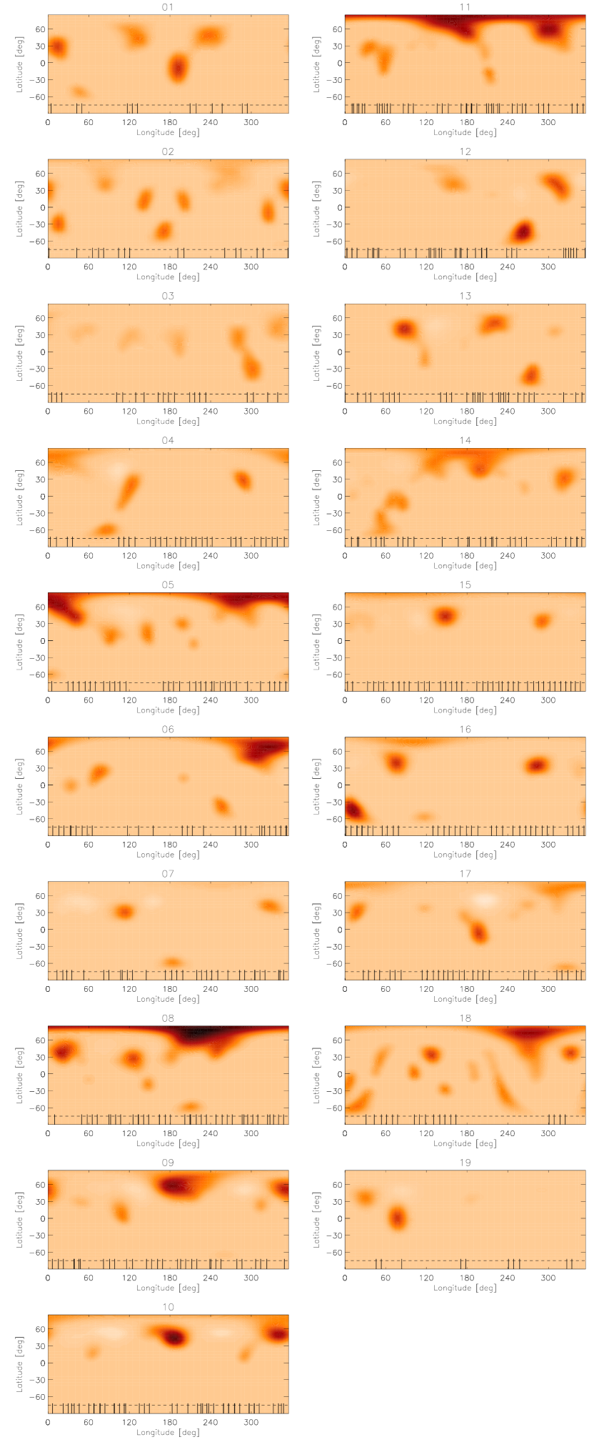
Figure 15: Doppler images S01-S10 (left, top to bottom) and S11-S19 (right, top to bottom) plotted in Mercator projection. The maps and the temperature scale correspond to those shown in Fig. 8. The ticks on the bottom edge indicate the phases of the observations used for that map.

Appendix E Spot filling factors

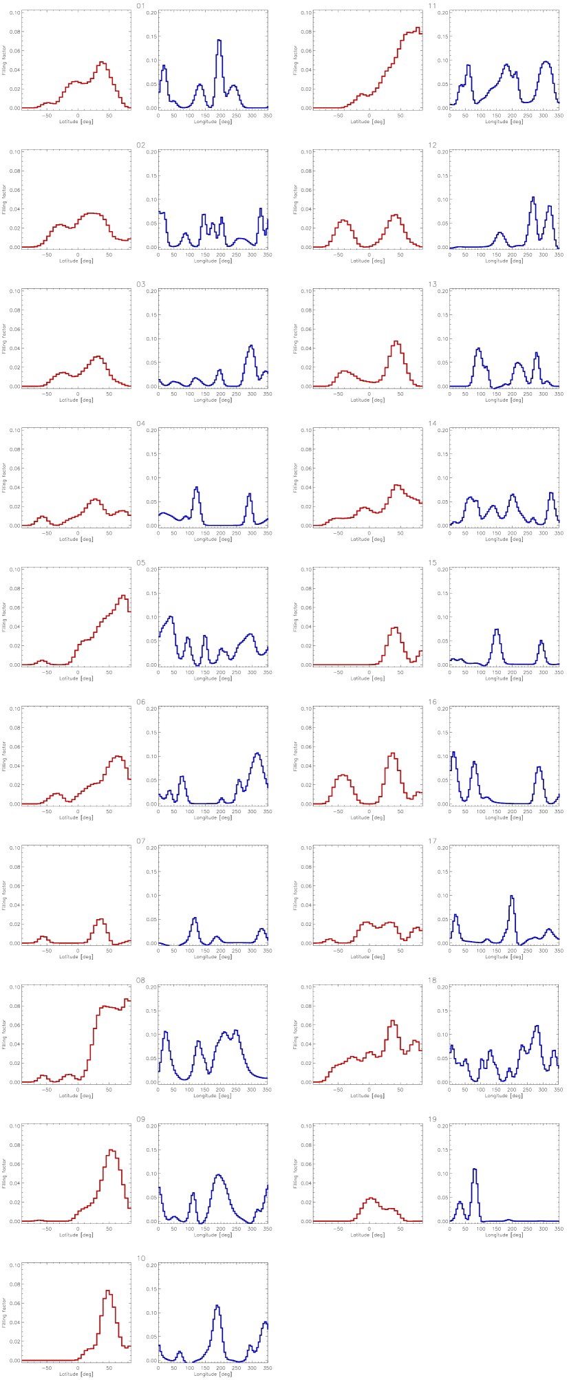
Figure 16: The spot filling factors for the nineteen Doppler images in the arrangement corresponding to Fig. 15. For each temperature map, the histogram of the spot filling factor is shown in two panels: on the left side (in red), summed along the latitude, and on the right side (in blue), summed up along the longitude.

Appendix F Measuring spot decay rate

Relying strictly on our time-series Doppler images, below we attempt to quantitatively measure the spot decay rate $\Delta A_{\rm s}/\Delta t_{\rm s}$ for V815 Her. For this we set up a simple statistic, in which we tracked the evolution of well-separated and easy-to-follow spots on our series of surface snapshots.

First, we identified spots on all 19 Doppler maps with the Photutils (Bradley et al. 2021) image segmentation function called detect_sources on the 72$\times$36 pixel images to detect spots below a specific threshold value. We required each spot to have at least ten pixels at least 50 K below the quiescent photosperic temperature. As a next step, we used the deblend_sources function to deblend the overlapping spots, with the minimum size of ten pixels. We ended up with 99 individual spots on all of the images. For each spot, we calculated the centroid position by weighting with temperature, and the area, taking into account the distortion of pixels with the cosine of the latitude. Then, we manually identified matching spots on consecutive image pairs. However, tracking decaying spots is made more difficult by interactions between neighboring spots (e.g. merging) or the emergence of new fluxes. Therefore, we only matched unambigous spot pairs, where it was reasonable to assume that we see the evolution of the same feature. The maximum allowed angular separation between the centroids of the subsequent images of the evolving spot was set to be 40^∘.

As an example, in Fig. 17 we show the identification of the individual spots for S01 and S02 Doppler images (top and middle panels, respectively) and the spot pairing (see the bottom panel). For each spot pair, we calculated the decay rate as $\Delta A/\Delta t$, where $\Delta A$ is the change in spot area, and $\Delta t$ is the time difference between the two images. The average decay rate for the 18 spot pairs showing negative $\Delta A$ (i.e. shrinking) is $\Delta A/\Delta t=-$7.0$\pm$1.3 10⁴ km² s^-1. For identification, we provide a list of these spots in Table F, while the list of spot pairs found on consecutive Doppler images that we considered to represent successive evolutionary phases (i.e. spot decay) of the same spot is as follows: #2$-$#11; #3$-$#12; #4$-$#10; #5$-$#13; #9$-$#16; #12$-$#18; #20$-$#23; #21$-$#25; #29$-$#34; #34$-$#37; #36$-$#40; #42$-$#45; #43$-$#48; #47$-$#52; #48$-$#53; #60$-$#63; #69$-$#75; #78$-$#83.

Finally, we note that the method is not mature, due to the aforementioned sources of error (e.g. interacting spots, arbitrarily taken threshold values, etc.), we consider it only suitable for order of magnitude estimation for the time being.

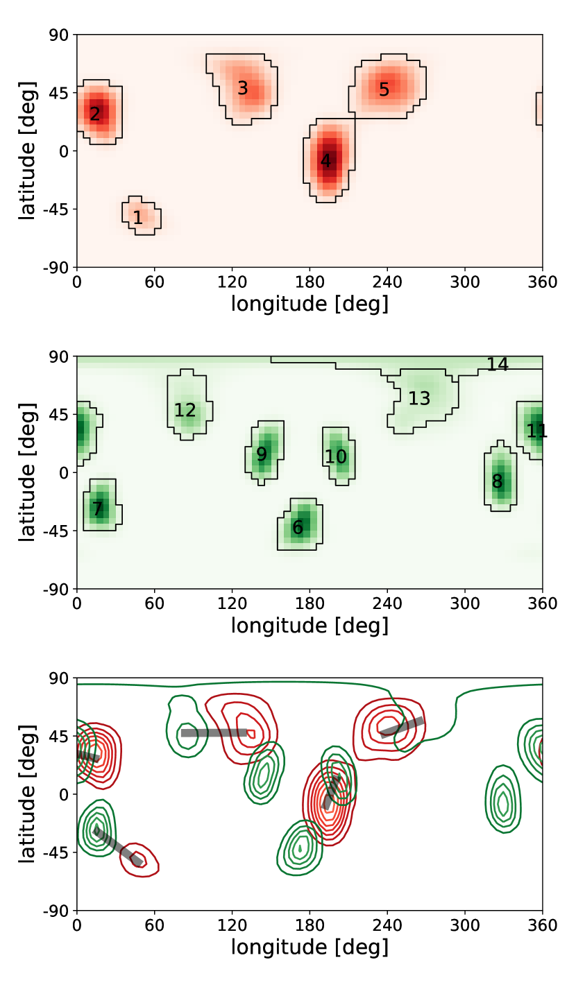
Figure 17: Demonstrating how spot segmentation and identification works. As an example, the upper panel shows the identified spots with their ID numbers (see also Table F) of the S01 Doppler image, and the middle one shows the identified spots of the S02 Doppler image. In the bottom panel, the spots of S01 are represented by red contours, the spots of S02 by green contour lines, and the paired spots are connected by gray lines.

Table 7: Identified spots with their longitude and latitude coordinates and their calculated area. In the last two columns, the equivalent spot radius and average temperature values are provided for information.

#	Image	$\lambda_{\rm s}$	$\beta_{\rm s}$	Area	$\overline{\gamma}_{\rm s}$	$\overline{T}_{\rm s}$
1	S01	47	$-$53	413	11.5	5469
2	S01	14	28	1414	21.2	5332
3	S01	128	48	1398	21.1	5420
4	S01	192	$-$9	2088	25.8	5303
5	S01	238	47	1542	22.2	5404
6	S02	171	$-$43	885	16.8	5387
7	S02	16	$-$29	895	16.9	5376
8	S02	325	$-$8	1135	19.0	5394
9	S02	143	13	1070	18.5	5394
10	S02	200	11	900	16.9	5405
11	S02	356	31	1230	19.8	5374
12	S02	84	47	854	16.5	5477
13	S02	265	56	1036	18.2	5488
14	S02	325	83	177	7.5	5486
15	S03	192	15	1016	18.0	5489
16	S03	120	24	766	15.6	5507
17	S03	342	45	1256	20.0	5473
18	S03	52	36	401	11.3	5520
19	S03	299	$-$27	1484	21.7	5394
20	S03	281	24	1245	19.9	5435
21	S04	85	$-$62	547	13.2	5420
22	S04	119	10	1728	23.5	5393
23	S04	288	28	959	17.5	5363
24	S04	14	70	1463	21.6	5435
25	S05	1	$-$61	305	9.9	5480
26	S05	215	$-$5	273	9.3	5474
27	S05	146	14	956	17.4	5417
28	S05	198	30	541	13.1	5436
29	S05	92	11	1296	20.3	5429
30	S05	32	64	2095	25.8	5132
31	S05	276	73	2074	25.7	5119
32	S06	257	$-$39	780	15.8	5399
33	S06	34	$-$1	570	13.5	5471
34	S06	75	20	1102	18.7	5390
35	S06	317	66	2505	28.2	5203
36	S07	184	$-$59	374	10.9	5444
37	S07	112	31	1020	18.0	5380
38	S07	328	41	756	15.5	5418
39	S07	252	80	22	2.7	5526
40	S08	210	$-$59	369	10.8	5443
41	S08	147	$-$18	478	12.3	5440
42	S08	125	26	1531	22.1	5354
43	S08	24	41	1715	23.4	5291
44	S08	234	72	3766	34.6	4917
45	S09	108	11	1153	19.2	5416
46	S09	48	29	252	9.0	5502
47	S09	314	25	480	12.4	5476
48	S09	351	52	1556	22.3	5308
49	S09	201	63	2411	27.7	5270
50	S10	261	$-$64	156	7.0	5502
51	S10	108	10	1158	19.2	5412
52	S10	316	25	458	12.1	5487
53	S10	353	51	1352	20.7	5357
54	S10	200	63	2531	28.4	5258
55	S11	213	$-$22	579	13.6	5430
56	S11	59	6	1444	21.4	5398
57	S11	36	26	883	16.8	5406
58	S11	201	74	3140	31.6	5020
59	S11	303	53	1877	24.4	5168
60	S12	262	$-$46	1487	21.8	5250
61	S12	313	39	1600	22.6	5331
62	S12	156	47	1138	19.0	5461
63	S13	275	$-$43	1083	18.6	5348
64	S13	219	49	1305	20.4	5366
65	S13	309	36	230	8.5	5497
66	S13	117	$-$10	775	15.7	5476
67	S13	89	38	1571	22.4	5328
68	S14	265	16	282	9.5	5509
69	S14	324	32	1451	21.5	5399
70	S14	54	$-$50	1093	18.6	5431
71	S14	76	$-$10	1460	21.6	5409
72	S14	201	49	1098	18.7	5325
73	S14	179	72	2054	25.6	5366
74	S15	148	44	1286	20.2	5325
75	S15	291	35	784	15.8	5384
76	S15	18	33	378	11.0	5521
77	S15	68	82	304	9.8	5439
78	S16	12	$-$46	1475	21.7	5223
79	S16	117	$-$57	263	9.2	5488
80	S16	284	35	1286	20.2	5294
81	S16	75	41	1343	20.7	5332
82	S16	99	79	411	11.4	5448
83	S17	326	$-$67	254	9.0	5479
84	S17	194	$-$0	2010	25.3	5367
85	S17	18	32	917	17.1	5392
86	S17	269	43	290	9.6	5503
87	S17	343	75	1067	18.4	5439
88	S18	234	$-$29	1830	24.1	5446
89	S18	147	$-$28	446	11.9	5430
90	S18	102	3	590	13.7	5395
91	S18	190	4	513	12.8	5486
92	S18	52	25	1011	17.9	5456
93	S18	128	34	954	17.4	5339
94	S18	19	$-$54	1180	19.4	5412
95	S18	4	$-$19	977	17.6	5415
96	S18	278	68	3152	31.7	5254
97	S18	333	37	923	17.1	5362
98	S19	78	1	1669	23.0	5329
99	S19	30	37	908	17.0	5422
degree
square degree
Kelvin