One-dimensional quantum scattering from multiple Dirac delta potentials: A Python-based solution

Abstract

In this paper, we present a Python-based solution designed to simulate a one-dimensional quantum system that incorporates multiple Dirac delta potentials. The primary aim of this research is to investigate the scattering phenomenon within such a system. By developing this program, we can generate wave functions throughout the system and compute transmission and reflection coefficients analytically and numerically for an infinite range of combinations involving potential strengths, distances, and the number of Dirac delta potentials. Furthermore, by modifying the code, we investigate transmission resonances, which yields the energy eigenvalues for particles undergoing perfect transmission through the quantum system. Subsequently, our research can be extended by considering impurities in the system. Finally, we attain the general analytical solution for transmission and reflection probabilities applicable to any number of potentials, and we possess the capability to generate variation plots that effectively explore the behavior of the system under scattering.

I Introduction

The Dirac delta potential has a profound impact on the field of science, with significant applications in various areas. For instance, the Kronig-Penny model stands out as a crucial example, as it effectively elucidates the formation of band gaps in crystal structuresE1 . The delta potential, often portrayed using the Dirac delta function, finds significant utility in quantum mechanics when describing interactions within systems of weakly interacting bosons. A prominent example of this application can be seen in the study of cold atomic gases, particularly in the context of Bose-Einstein condensates. In this context, the delta potential serves as a mathematical tool to model the localized potential energy at a specific point or region in space, which characterizes the interaction between the weakly interacting bosons.E2 . Indeed, the concept of delta potentials and their successful applications have led to significant research in various areas of physics. One noteworthy study in this domain demonstrates that scattering and reflection amplitudes of an arbitrary potential can be approximated using delta potentials E3 ; E4 . In recent years, there has been a growing interest in the study of one-dimensional systems featuring multiple Dirac delta potentials. Researchers have applied transfer matrix techniques to explore fascinating scattering phenomena, including transmission resonances (occurring at energies with a transmission coefficient of one), threshold anomalies (where the reflection coefficient approaches zero under certain parameter conditions as the incoming particle’s energy approaches zero), and the investigation of Bloch states. These investigations have significantly advanced our comprehension of wave behavior and particle interactions within such systems E6 ; E7 ; E8 ; E9 ; E10 ; E11 . An important feature of Dirac delta potentials is their exact solvability, which renders them highly suitable for educational purposes. Reference E12 offers insights into Green’s functions and the solution of the Lippmann-Schwinger equation for a single Dirac delta potential. Furthermore, reference E13 takes a pedagogical approach to explore multiple scattering theory for double delta centers using the Lippmann-Schwinger equation. These educational materials contribute to a deeper understanding of fundamental quantum mechanics and scattering theory concepts. A recent review E3 has shed light on some fascinating characteristics of one-dimensional Dirac delta potentials. It specifically explores the spectrum of both continuum and bound states within delta potentials, as well as other potentials amenable to exact solutions. Moreover, the review delves into the study of multiple delta-function potentials in Fourier space and frames the bound state problem in terms of a matrix eigenvalue problem.

In this study, we initiate our exploration by representing the Schrödinger equation in a dimensionless form. Furthermore, we revisit the topic of scattering, specifically focusing on both single and double Dirac delta potentials in Section 2. Subsequently, our study advances to the simulation of a system consisting of multiple one-dimensional Dirac delta potentials using Python. This program exhibits remarkable versatility, accommodating any desired number of potentials. Our focus then shifts towards enhancing the program’s capabilities by modifying the code to generate regional wavefunctions. By imposing appropriate boundary conditions at each potential point, we establish a system of equations that allows us to determine transmission and reflection coefficients. This fundamental analysis forms the basis for understanding the behavior of quantum particles in our system. To further enrich our investigation, we extend our code to explore transmission resonances within the system. This extension enables us to obtain exact eigenvalues for the particle’s energy at which perfect transmission occurs, shedding light on critical aspects of the system’s behavior. Additionally, by generalizing the code, we delve into the study of impurities within the system. This generalized approach enables us to investigate how impurities impact the behavior of quantum particles in the presence of multiple Dirac delta potentials. This exploration deepens our understanding of real-world scenarios where imperfections and variations exist. we bring together the comprehensive insights gained from our simulations and analyses to provide a general analytical solution for transmission and reflection probabilities in the context of scattering from multiple Dirac delta potentials in Section 4.

The combination of theoretical and computational methods showcased in this study serves as a powerful model for approaching complex quantum systems, providing a stepping stone for researchers to tackle even more intricate problems.

II Revisiting scattering from single and double Dirac delta potential

Figure 1: Scattering from a single Dirac delta potential: The sign of the potential strength determines whether the system consists of a well or a barrier.

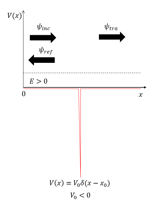
In this section, we consider the Schrödinger equation with a Dirac delta potential $V(x)=V_{0}\delta(x-x_{0})$ as shown in figure 1. Furthermore, we initiate the process of making the Schrödinger equation dimensionless by introducing a new variable, $y=kx$ in which $k^{2}=\frac{2mE}{\hbar}$. By applying this transformation, we aim to express the Schrödinger equation in a dimensionless form. Subsequently, we discuss the scattering problem, to determine the transmission and reflection coefficients associated with the system. Starting from the Schrödinger equation

$$-\frac{\hbar^{2}}{2m}\frac{d^{2}\psi}{dx^{2}}-V_{0}\delta(x-x_{0})\psi=E\psi,$$ (1)

and substituting the new variable $y=kx$, and constants $k^{2}=\frac{2mE}{\hbar^{2}}$, and $\tilde{V_{0}}=\frac{2mV_{0}}{\hbar^{2}}$ simplifies Eq. (1‘) as follows:

$$-\frac{d^{2}\psi}{dy^{2}}-\xi\delta(y-y_{0})\psi=\psi,$$ (2)

where $\xi=\frac{\tilde{V_{0}}}{k}$. By integrating both sides of (2) from $y_{0}-\epsilon$ to $y_{0}+\epsilon$ and by taking it’s limit as $\epsilon$ goes to zero we obtain

$$\frac{d\psi{}_{R}}{dy}(y_{o})-\frac{d\psi{}_{L}}{dy}(y_{o})=-\xi\psi(y_{0}).$$ (3)

The latter equation shows the behavior of the wave functions at the boundary. Here the $\frac{d\psi{}_{R}}{dy}(y_{o})$ represent the derivative of the wave function from the right-hand side and $\frac{d\psi{}_{L}}{dy}(y_{o})$ is the derivative of wave function from the left-hand side. Now by solving the Schrödinger equation at the regions of $y<y_{0}$ and $y_{0}<y$, we get the following result:

$$\psi_{L}=\exp(iy)+r\exp(-iy),$$ (4)

and

$$\psi_{R}=t\exp(iy),$$ (5)

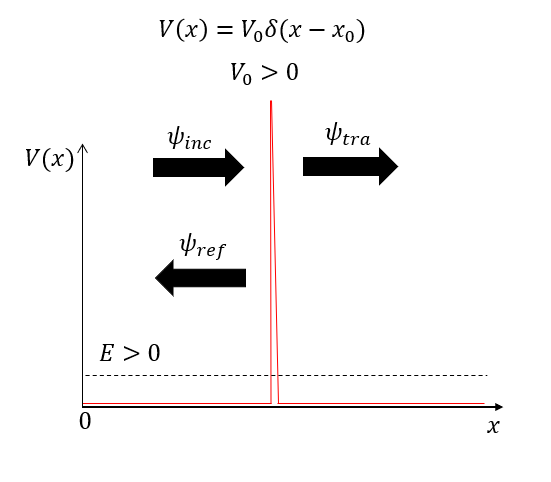
in which $r$ and $t$ are the reflection and transmission coefficients. By applying the continuity conditions of the wave function at the boundary $y=y_{0}$, and the discontinuity conditions (3), we determine the transmission and reflection coefficients, which are expressed by

Figure 2: Scattering from a double Dirac potential well separated by a distance $d$.

$$t=\frac{2i}{\xi+2i},$$ (6)

and

$$r=\frac{-\xi\exp(2iy_{0})}{\xi+2i}.$$ (7)

the conservation of the particle implies the condition $\mid t\mid^{2}+\mid r\mid^{2}=1$, where $\mid t\mid^{2}$ and $\mid r\mid^{2}$ are the probability of transmission and reflection of a particle undergoing the single Dirac delta potential.

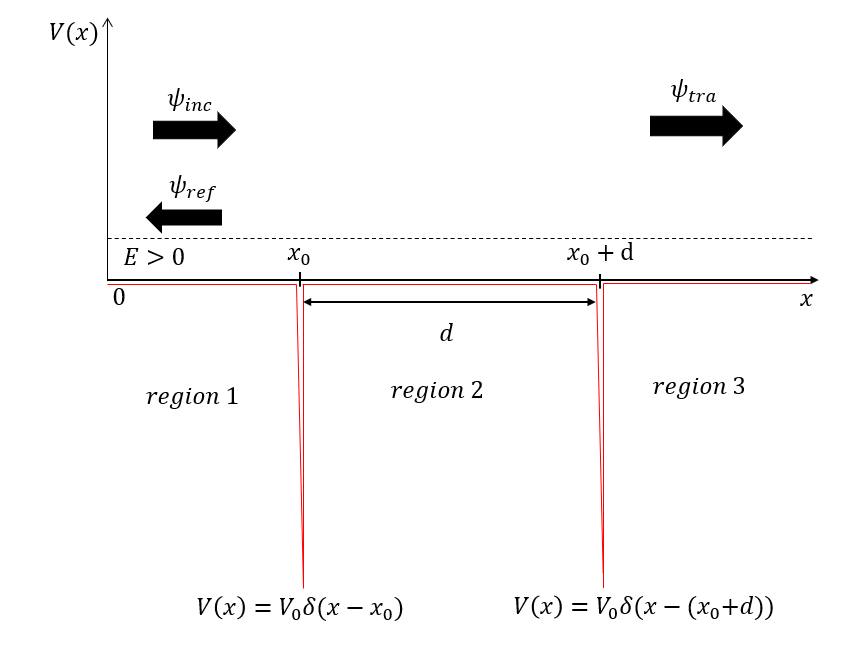
By employing identical procedures as illustrated for Figure 2, while setting $y_{0}=0$ and maintaining a separation of $d$ with a specified potential strength $V_{0}$, and subsequently applying the second boundary condition at the second potential, while setting $d_{t}=kd$, we derive the solutions for transmission and reflection coefficients as follows:

$$t=\frac{4}{\xi^{2}(\exp(2id_{t})-1)-4(i\xi-1)},$$ (8)

and

$$r=\frac{\xi^{2}(1-\exp(2id_{t}))+2i\xi(\exp(2id_{t})+1)}{\xi^{2}(\exp(2id_{t})-1)-4(i\xi-1)}.$$ (9)

III Scattering from multiple Dirac delta potentials: Python solution

The issue arises when attempting to generalize the system to encompass multiple Dirac delta potentials. Analyzing scattering in such a system can become tedious and time-consuming. Solving the Schrödinger equation throughout the system entails the application of continuity and discontinuity boundary conditions at each potential site. This process necessitates solving a system of equations to determine the transmission and reflection coefficients. In this section, we create a Python program to explore the one-dimensional scattering phenomenon involving multiple Dirac delta potentials, categorized into four different scenarios. These categories include examining whether the system has equidistantly spaced potentials or not, whether the potentials are of equal strength, or if they contain impurities.

III.1 Wave functions and IVP

In this section, following the inclusion of the essential libraries, we commence by crafting a one-dimensional quantum system featuring multiple Dirac delta potentials. Subsequently, one may determine if the system can be uniformly distributed or if an arbitrary distribution is preferred. To initiate the system, the first step involves establishing the initial values, namely the potential_list, and distance_list. The program itself is implemented as a user input program, offering various options to the user. Initially, the user is presented with a choice between equal distances or non-equal distances, as well as equal potentials or non-equal potentials. Furthermore, the user is prompted to input the value of $k$. With these inputs at hand, we proceed to compute the $\xi$ list. as shown in the below code: These options allow for flexibility in defining the characteristics of the generated multiple Dirac delta potentials.

⬇

potential_list = []

distance_list=[]

num_potential = int(input("Enter the number of potentials: "))

potential_types = input("choose between ’equal potentials’ or ’non equal potentials’: ").lower()

distance_types=input("choose between ’equal distances’ or ’non equal distances’: ").lower()

if potential_types == ’non equal potentials’:

for i in range(num_potential):

value_of_potential = float(input("Enter the value of potential {}: ".format(i+1)))

potential_list.append(value_of_potential)

elif potential_types == ’equal potentials’:

value_of_potential = float(input("Enter the value of potential: "))

potential_list = [value_of_potential] * num_potential

else:

print("Invalid potential types!")

if distance_types==’non equal distances’:

for i in range(num_potential-1):

value_of_distance=float(input("Enter the value of distance {}: ".format(i+1)))

distance_list.append(value_of_distance)

elif distance_types==’equal distances’:

value_of_distance = float(input("Enter the value of distance: "))

distance_list = [value_of_distance] * int((num_potential-1))

else:

print("Invalid distance types!")

def divide_list_elements(lst, divisor):

new_lst = [num / divisor for num in lst]

return new_lst

k = int(input("enter value of k: "))

kisi_f = divide_list_elements(potential_list,k)

Once you have selected your preferred option and set the initial values, such as $\xi$ and distances, the code will initiate by providing you with a list of general wave functions and their corresponding derivatives as functions of $y$. You can observe this in the following code:

⬇

A = [smp.symbols("a{}".format(i)) for i in range(1, num_potential + 2)]

B = [smp.symbols("b{}".format(i)) for i in range(1, num_potential + 2)]

t, r,y=smp.symbols("t r y")

B[0] = r

A[0] = 1

B[num_potential] = 0

A[num_potential] = t

psi_y = [A[i] * smp.exp(1j*y) + B[i] * smp.exp(-1j* y) for i in range(num_potential+1)]

print("wave functions in our system is as followes:")

print(psi_y)

dpsi_y = []

for i in range(num_potential + 1):

derivative = smp.diff(psi_y[i],y)

dpsi_y.append(derivative)

print("derivatives of wave functions are as followes:")

print(dpsi_y)

III.2 Boundary Conditions

Once the wave functions and their corresponding derivatives have been compiled into a list, it is crucial to independently apply the continuity boundary condition for each distinct region, considering both equal and non-equal distances. The same method is followed to formulate the boundary condition for the derivatives of wave functions within each region, as depicted in the following code:

⬇

bc_eq1=[]

privious_psi_y=psi_y[0]

for element in psi_y[1:]:

difference=element-privious_psi_y

bc_eq1.append(difference)

privious_psi_y=element

list_of_distances=[]

D_t=[smp.symbols("d_t{}".format(i)) for i in range(1,num_potential )]

if distance_types==’equal distances’:

for i in range(num_potential):

y= y0 + n*d_t

result= y.subs([(y0,y0_n),(n,i)])

list_of_distances.append(result)

elif distance_types==’non equal distances’:

list_of_distances = [y0_n] + [y0_n+ smp.Add(*D_t[:i]) for i in range(1, num_potential)]

y = smp.symbols(’y’)

n = num_potential

y_symbols = smp.symbols(’y1:{}’.format(n + 1))

bc_eq1_indexed = [eq.subs(y, y_sym) for eq, y_sym in zip(bc_eq1,y_symbols)]

bc_eq1_n=[]

for i in range(len(list_of_distances)):

if distance_types==’equal distances’:

y_index1 = i + 1

y_value1 = list_of_distances[i]

bc_eq1_n.append(bc_eq1_indexed[i].subs(f’y{y_index1}’,y_value1))

elif distance_types==’non equal distances’:

y_index1 = i + 1

y_value1 = list_of_distances[i]

bc_eq1_n.append(bc_eq1_indexed[i].subs(f’y{y_index1}’,y_value1))

print(bc_eq1_n)

bc_eq2 = []

previous_dpsi_y = dpsi_y[0]

previous_psi_y2 = psi_y[1]

for i in range(1, len(dpsi_y)):

if potential_types == ’equal potentials’:

kisi=smp.symbols("kisi")

current_dpsi_y = dpsi_y[i]

current_psi_y = psi_y[i]

difference = current_dpsi_y - previous_dpsi_y + (kisi) * current_psi_y

bc_eq2.append(difference)

previous_dpsi_y = current_dpsi_y

previous_psi_y2 = current_psi_y

elif potential_types == ’non equal potentials’:

kisi_list = [smp.symbols("kisi{}".format(i)) for i in range(1, num_potential+1)]

kisi=smp.symbols("kisi")

current_dpsi_y = dpsi_y[i]

current_psi_y = psi_y[i]

difference = current_dpsi_y - previous_dpsi_y + kisi_list[i-1] * current_psi_y

bc_eq2.append(difference)

previous_dpsi_y = current_dpsi_y

previous_psi_y2 = current_psi_y

print(bc_eq2)

y = smp.symbols(’y’)

n = num_potential

y_symbols = smp.symbols(’y1:{}’.format(n + 1))

bc_eq2_indexed = [eq.subs(y, y_sym) for eq, y_sym in zip(bc_eq2, y_symbols)]

print(bc_eq2_indexed )

bc_eq2_n= []

for i in range(len(list_of_distances)):

if distance_types==’equal distances’:

y_index = i + 1

y_value = list_of_distances[i]

bc_eq2_n.append(bc_eq2_indexed[i].subs(f’y{y_index}’, y_value))

elif distance_types==’non equal distances’:

y_index = i + 1

y_value = list_of_distances[i]

bc_eq2_n.append(bc_eq2_indexed[i].subs(f’y{y_index}’, y_value))

print(bc_eq2_n)

III.3 Transmission and Reflection Coefficient

Now that we have symbolically defined the boundary conditions for any variation in our user may request, and we have obtained the initial values of $\xi$ and distances, the next step is to import these values and construct a system of equations. Once the system is formed, we can proceed to solve it effectively Once the solutions for each coefficient in every region have been obtained, allowing for user-defined variations in the wave functions, and the reflection and transmission coefficients have been evaluated, the next step is to analyze the probability invariant. Additionally, you can assign the coefficients to the wave functions to calculate their conjugates as well as the absolute value of the wave functions. The code below illustrates how to perform these tasks:

⬇

if distance_types==’non equal distances’:

new_list = [expr.subs(zip(D_t, distance_list)) for expr in bc_eq1_n]

elif distance_types==’equal distances’:

distance_list_sympy = [smp.sympify(element) for element in distance_list]

substitutions = [(d_t, value) for value in distance_list_sympy]

new_list = [expr.subs(substitutions) for expr in bc_eq1_n]

if distance_types==’non equal distances’ and potential_types==’non equal potentials’:

new_list2 = [expr.subs(zip(kisi_list, kisi_f)) for expr in bc_eq2_n]

new_list3 =[expr.subs(zip(D_t, distance_list)) for expr in new_list2]

elif distance_types==’equal distances’ and potential_types==’non equal potentials’:

distance_list_sympy = [smp.sympify(element) for element in distance_list]

substitutions = [(d_t, value) for value in distance_list_sympy]

new_list2 = [expr.subs(substitutions) for expr in bc_eq2_n]

new_list3 = [expr.subs(zip(kisi_list, kisi_f)) for expr in new_list2]

elif distance_types==’non equal distances’ and potential_types==’equal potentials’:

potential_list_sympy = [smp.sympify(element) for element in kisi_f]

substitutions = [(kisi, value) for value in potential_list_sympy]

new_list2 = [expr.subs(substitutions) for expr in bc_eq2_n]

new_list3 =[expr.subs(zip(D_t, distance_list)) for expr in new_list2]

elif distance_types==’equal distances’ and potential_types==’equal potentials’:

distance_list_sympy = [smp.sympify(element) for element in distance_list]

substitutions = [(d_t, value) for value in distance_list_sympy]

new_list2 = [expr.subs(substitutions) for expr in bc_eq2_n]

potential_list_sympy = [smp.sympify(element) for element in kisi_f]

substitutions = [(kisi, value) for value in potential_list_sympy]

new_list3 = [expr.subs(substitutions) for expr in new_list2]

system_of_equations = [Eq(eq, 0) for eq in (new_list + new_list3)]

print(system_of_equations)

symbols_list = list(set().union(*[eq.free_symbols for eq in system_of_equations]))

solution = solve(system_of_equations, symbols_list)

symbol_values = {symbol: value for symbol, value in solution.items()}

print("Assigned Values:")

for symbol, value in symbol_values.items():

print(f"{symbol}: {value}")

functions = {}

for symbol, value in symbol_values.items():

func = smp.lambdify([], value)

functions[symbol] = func

r_value = functions[r]()

t_value=functions[t]()

ai=[]

bi=[]

for i in range(2, num_potential+1):

a_value = functions[A[i-1]]()

ai.append(a_value)

b_value = functions[B[i-1]]()

bi.append(b_value)

print(f"a{i} value: {a_value}")

print(f"b{i} value: {b_value}")

probability_invariance=Abs(t_value)**2+Abs(r_value)**2

print(probability_invariance)

substituted_psi_y = []

for expr in psi_y:

substituted_expr = expr.subs({’r’: r_value, ’t’: t_value})

for i in range(0,num_potential-1):

substituted_expr = substituted_expr.subs({A[i+1]: ai[i],B[i+1]: bi[i]})

substituted_psi_y.append(substituted_expr)

print(substituted_psi_y)

conjugate_psi_y1 = [conjugate(expr) for expr in substituted_psi_y]

conjugate_psi_y = [expr.subs(conjugate(y), y) for expr in conjugate_psi_y1]

print(conjugate_psi_y)

psi_y_square = [expand(expr1 * expr2) for expr1, expr2 in zip(substituted_psi_y, conjugate_psi_y)]

abs_psi_y_square = [Abs(expr).rewrite(Abs) for expr in psi_y_square]

print(abs_psi_y_square)

As an example, let’s consider a system containing double Dirac delta potentials with the following properties: $n=2$, $\tilde{V_{0}}=1$, $d=1$, and $k=1$ by executing the code, we obtain the following wave functions and their corresponding derivatives within both Region 1 and Region 3. This outcome reflects the results of the implemented procedures, allowing for a clear examination of the wave functions and their derivatives in these specific regions.

$$\psi_{1}(y)=\exp(iy)+r\exp(-iy),$$ (10)

$$\frac{d\psi_{1}}{dy}=i\exp(iy)-ir\exp(-iy),$$ (11)

$$\psi_{3}(y)=t\exp(iy),$$ (12)

and

$$\frac{d\psi_{3}}{dy}=it\exp(iy).$$ (13)

The provided code executes boundary conditions at the potential sites, inserts initial values, and constructs a system of equations as follows:

$$a_{2}+ia_{2}+b_{2}-ib_{2}+ir-i=0,$$ (14)

$$-ia_{2}\exp(i)+ib_{2}\exp(-i)+it\exp(i)+t\exp(i)=0,$$ (15)

$$ia_{2}-ib_{2}+\xi(a_{2}+b_{2})+ir-i=0,$$ (16)

and

$$-ia_{2}\exp(i)+ib_{2}\exp(-i)+\xi t\exp(i)+it\exp(i).$$ (17)

Moreover, the code solves the system of equations to compute the coefficients and determine the transmission and reflection coefficients. This calculation is essential for a comprehensive understanding of the system’s behavior and how it responds to the given properties and potential sites. The code serves as a valuable tool for obtaining these numerical which are as follows:

$$r=-0.113288627686634-0.0355022314425367i,$$ (18)

$$t=0.636858618114342+0.761784995213854i,$$ (19)

$$a_{2}=1.01775111572127+0.443355686156683i,$$ (20)

and

$$b_{2}=-0.131039743407903-0.47885791759922i.$$ (21)

The conservation of the particle is also satisfied $\mid t\mid^{2}+\mid r\mid^{2}=1$

III.4 Graphical Representation and Transmission Resonance

In this section, we begin by introducing a well-defined structure for scattering within a user-designed system by incorporating the coefficient values into the wave function. Subsequently, we divide our code into three distinct components, each addressing different scenarios: whether the potentials are uniformly distributed with consistent magnitudes or if the potential distribution is uniform but marred by impurities within the system. By defining a range for each distinct category, the code will plot the wave functions and their absolute values concerning the regional distances between each potential site. Then, by analytically solving the system of equations governing boundary conditions, we can obtain solutions for the transmission and reflection coefficients for any number of potential sites. This enables us to create graphical representations based on transmission and reflection probabilities with respect to their distances and energy. Additionally, we can identify the exact eigenvalue for the energy of the particle to achieve perfect transmission.

III.4.1 Equal distances and Equal potentials

Initially, we proceed by inserting the values of coefficients into each regional wave function. Then, we define a range for our scattering phenomena, which includes potentials at user-defined distances. The code will then plot the wave functions and the absolute value of the wave function squared through scattering phenomena, as shown below:

⬇

if potential_types == ’equal potentials’and distance_types == ’equal distances’:

lambdified_psi_y_functions = [lambdify(y, func) for func in substituted_psi_y]

l = num_potential-1 # Define the value of n

range_of_graph = [] # Initialize an empty list to store the ranges

start = y0_n - (10 * value_of_distance)

end = y0_n

range_of_graph.append((start, end)) # Add the first range

for i in range(l):

start = y0_n + (i * value_of_distance)

end = y0_n + ((i+1) * value_of_distance)

range_of_graph.append((start, end))

end = y0_n + ((l + 10) * value_of_distance)

range_of_graph.append((y0_n + (l * value_of_distance), end)) # Add the last range

print(range_of_graph)

plt.figure(1)

for i, func in enumerate(lambdified_psi_y_functions):

y_vals = np.linspace(range_of_graph[i][0], range_of_graph[i][1], 1000)

f_vals = np.real(func(y_vals))

plt.plot(y_vals, f_vals, label=str(substituted_psi_y [i]))

plt.xlabel(’y’)

plt.ylabel(’psi_y’)

plt.title(’Plot of wave function’)

lambdified_abs_psi_y_square = [lambdify(y, func) for func in abs_psi_y_square]

m = num_potential - 1

range_of_graph1 = []

start1 = y0_n - (10 * value_of_distance)

end1 = y0_n

range_of_graph1.append((start1, end1))

for i in range(m):

start1 = y0_n + (i * value_of_distance)

end1 = y0_n + ((i + 1) * value_of_distance)

range_of_graph1.append((start1, end1))

end1 = y0_n + ((m + 10) * value_of_distance)

range_of_graph1.append((y0_n + (m * value_of_distance), end1))

plt.figure(2)

for i, func in enumerate(lambdified_abs_psi_y_square):

y_vals1 = np.linspace(range_of_graph1[i][0], range_of_graph1[i][1], 1000)

f_vals1 = np.vectorize(func)(y_vals1)

plt.plot(y_vals1, np.real(f_vals1), label=str(abs_psi_y_square[i]))

plt.xlabel(’y’)

plt.ylabel(’psi_y_square’)

plt.title(’Plot of abs wave function square’)

plt.grid(True)

plt.show()

As we progress with the code, our initial step involves solving the system of equations analytically to obtain the transmission and reflection coefficients, considering the parameters of $d_{t}$ and $\xi$. Subsequently, we visualize the scattering behavior of particles by plotting the transmission and reflection probabilities, as demonstrated in the code below:

⬇

system_of_equations_algebric = [Eq(eq, 0) for eq in (bc_eq1_n + bc_eq2_n)]

symbols_list_algebric = list(set().union(*[eq.free_symbols for eq in system_of_equations_algebric]))

solution_algebric = smp.solve(system_of_equations_algebric, symbols_list)

symbol_values_algebric = {symbol: value for symbol, value in solution_algebric.items()}

print(symbol_values_algebric)

r_value_algebric = symbol_values_algebric[r]

t_value_algebric = symbol_values_algebric[t]

r_func = lambdify((d_t, kisi), r_value_algebric, modules=’numpy’)

t_func = lambdify((d_t, kisi), t_value_algebric, modules=’numpy’)

# Define the range of kisi and d_t values

kisi_values = np.linspace(0, kisi_f, 100)

d_t_values = np.linspace(0, distance_list[0], 100)

# Create a meshgrid of kisi and d_t values

kisi_mesh, d_t_mesh = np.meshgrid(kisi_values, d_t_values)

abs_r_product = np.abs(r_func(d_t_mesh, kisi_mesh) * np.conj(r_func(d_t_mesh, kisi_mesh)))

abs_t_square = np.abs(t_func(d_t_mesh, kisi_mesh) * np.conj(t_func(d_t_mesh, kisi_mesh)))

fig = plt.figure(figsize=(10,8))

ax = fig.add_subplot(111, projection=’3d’)

ax.plot_surface(kisi_mesh, d_t_mesh, abs_r_product, cmap=’viridis’)

ax.plot_surface(kisi_mesh, d_t_mesh, abs_t_square, cmap=’magma’)

ax.set_xlabel(’kisi’)

ax.set_ylabel(’d_t’)

ax.set_zlabel(’Magnitude’)

ax.set_title(’Absolute square of r and t’)

kisi=kisi_f[0]

d_t_values1=np.linspace(0,10,1000)

abs_r_product_kisi = np.abs(r_func(d_t_values1, kisi) * np.conj(r_func(d_t_values1, kisi)))

abs_t_square_kisi = np.abs(t_func(d_t_values1, kisi) * np.conj(t_func(d_t_values1, kisi)))

fig, ax = plt.subplots(figsize=(8, 6))

ax.plot(d_t_values1, abs_r_product_kisi, label=’|r|^2’)

ax.plot(d_t_values1, abs_t_square_kisi, label=’|t|^2’)

ax.set_xlabel(’d_t’)

ax.set_ylabel(’Magnitude’)

ax.set_title(’Absolute square of r and t for kisi = {}’.format(kisi))

ax.legend()

kisi=np.linspace(0,10,1000)

d_t_values1=distance_list[0]

abs_r_product_kisi = np.abs(r_func(d_t_values1, kisi) * np.conj(r_func(d_t_values1, kisi)))

abs_t_square_kisi = np.abs(t_func(d_t_values1, kisi) * np.conj(t_func(d_t_values1, kisi)))

fig, ax = plt.subplots(figsize=(8, 6))

ax.plot(kisi, abs_r_product_kisi, label=’|r|^2’)

ax.plot(kisi, abs_t_square_kisi, label=’|t|^2’)

ax.set_xlabel(’kisi’)

ax.set_ylabel(’Magnitude’)

ax.set_title(’Absolute square of r and t for d_t = {}’.format(distance_list[0]))

ax.legend()

plt.show()

When executing the provided code with the settings of ’equal potentials,’ ’equal distances,’ and a specified count of 6 potential instances, firstly the analytical solution for transmission and reflection coefficient is as follows:

$$t=\frac{\alpha_{0}}{\sum_{i=0}^{6}\xi^{i}\alpha_{i}},$$ (22)

$$r=\frac{\sum_{i=1}^{6}\xi^{i}\beta_{i}}{\sum_{i=0}^{6}\xi^{i}\alpha_{i}},$$ (23)

$$\alpha_{0}=64,$$ (24)

$$\alpha_{1}=-192i,$$ (25)

$$\alpha_{2}=80e^{2id_{t}}+64e^{4id_{t}}+48e^{6id_{t}}+32e^{8id_{t}}+16e^{10id_{t}}-240,$$ (26)

$$\alpha_{3}=-160ie^{2id_{t}}-64ie^{4id_{t}}+32ie^{8id_{t}}+32e^{10id_{t}}+160i,$$ (27)

$$\alpha_{4}=-120e^{2id_{t}}+24e^{4id_{t}}+48e^{6id_{t}}+12e^{8id_{t}}-24e^{10id_{t}}+60,$$ (28)

$$\alpha_{5}=40ie^{2id_{t}}-40ie^{4id_{t}}+20ie^{8id_{t}}-8ie^{10id_{t}}-12i,$$ (29)

$$\alpha_{6}=5e^{2id_{t}}-10e^{4id_{t}}+10e^{6id_{t}}-5e^{8id_{t}}+e^{10id_{t}}-1,$$ (30)

$$\beta_{1}=32ie^{2id_{t}}+32ie^{4id_{t}}+32ie^{6id_{t}}+32ie^{8id_{t}}+32ie^{10id_{t}}+32i,$$ (31)

$$\beta_{2}=48e^{2id_{t}}+16e^{4id_{t}}-16e^{6id_{t}}-48e^{8id_{t}}-80e^{10id_{t}}+80,$$ (32)

$$\beta_{3}=16ie^{2id_{t}}+64ie^{4id_{t}}+64ie^{6id_{t}}+16ie^{8id_{t}}-80ie^{10id_{t}}-80i,$$ (33)

$$\beta_{4}=56e^{2id_{t}}+32e^{4id_{t}}-32e^{6id_{t}}-56e^{8id_{t}}+40e^{10id_{t}}-40,$$ (34)

$$\beta_{5}=-30ie^{2id_{t}}+20ie^{4id_{t}}+20ie^{6id_{t}}-30ie^{8id_{t}}+10ie^{10id_{t}}+10i,$$ (35)

and

$$\beta_{6}=-5e^{2id_{t}}+10e^{4id_{t}}-10e^{6id_{t}}+5e^{8id_{t}}-e^{10id_{t}}+1.$$ (36)

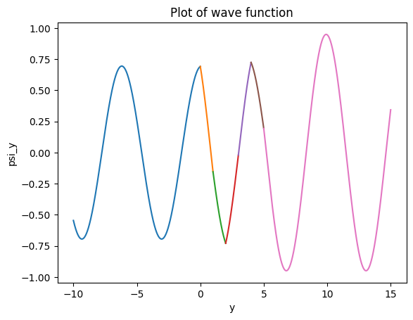
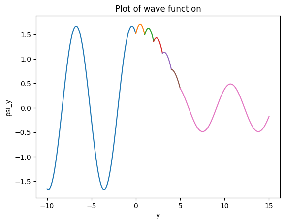
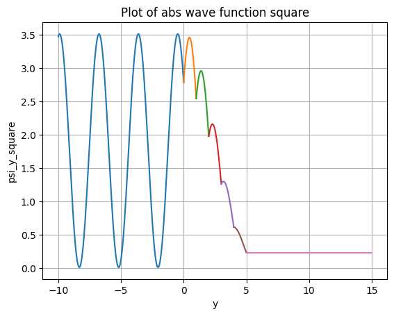
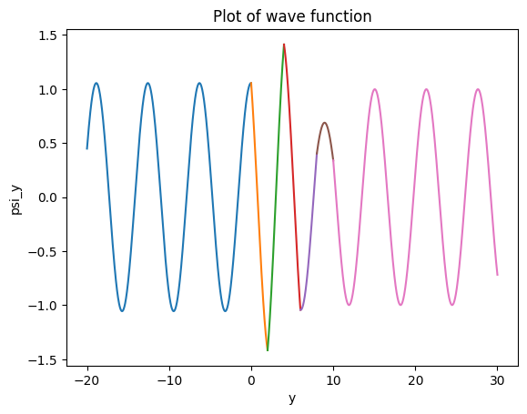
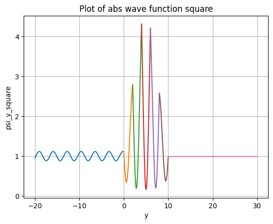
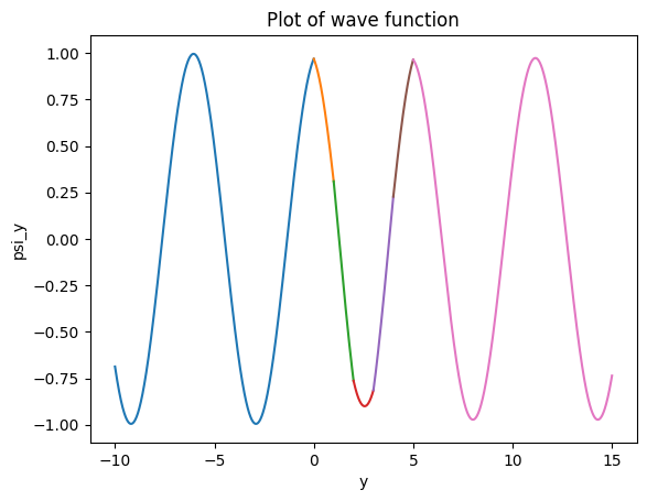
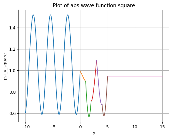
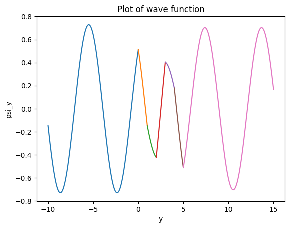
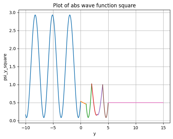
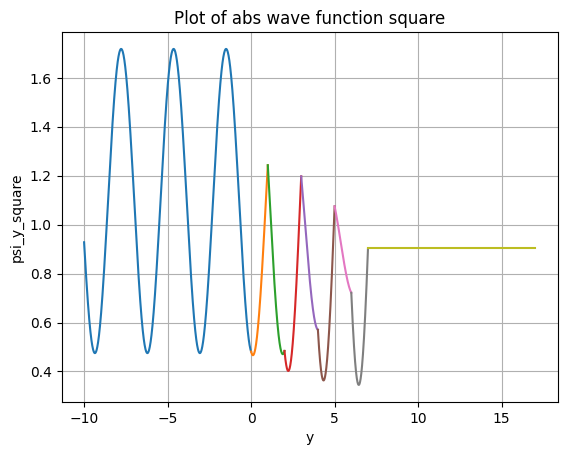
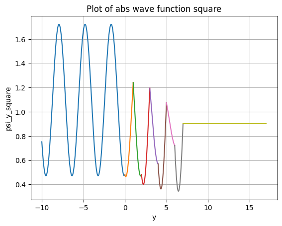
Now, by initializing the parameters as $\tilde{V}=1$, $k=1$, and $y_{0}=0$,’ the program will analyze and visualize the scattering phenomenon, as demonstrated in figures 3 and 4.it’s important to note the increased amplitude of the wave functions after scattering, which is due to representing only the real part of the graph. Upon closer examination, the absolute value of the wave function transforms into a straight line post-scattering. This behavior is a result of applying boundary conditions, which require the last coefficient of the wave function to approach zero as y approaches infinity. As a result, squaring the absolute value yields the transmission probability, consistently less than 1. The numerical values for transmission and reflection probabilities for this particular case are as follows

Figure 3: Plots of wave function and its absolute value squared for $\tilde{V}=1$, $k=1$, and $y_{0}=0$.

Figure 4: plots of transmission and reflection probability in terms of $y$ and $\xi$.

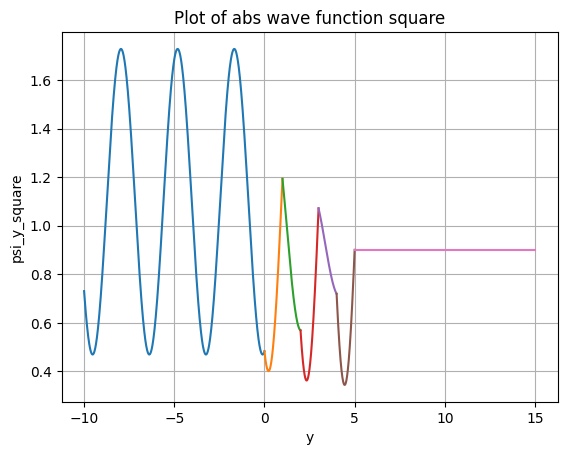
$$\mid t\mid^{2}=0.23624786700649963,$$ (37)

and

$$\mid r\mid^{2}=0.7637521329935002.$$ (38)

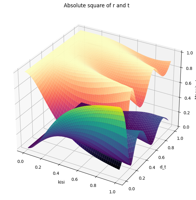
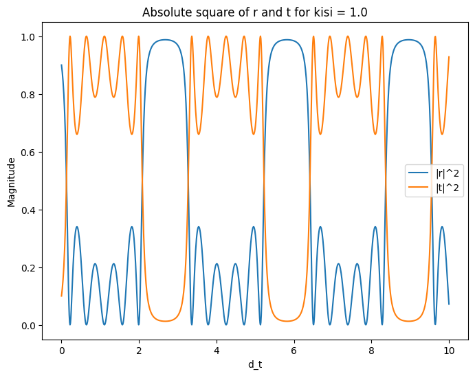
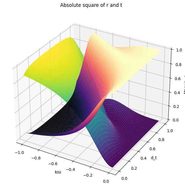
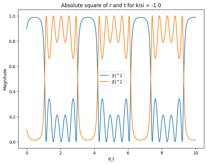
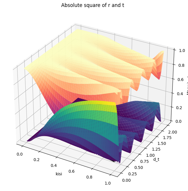
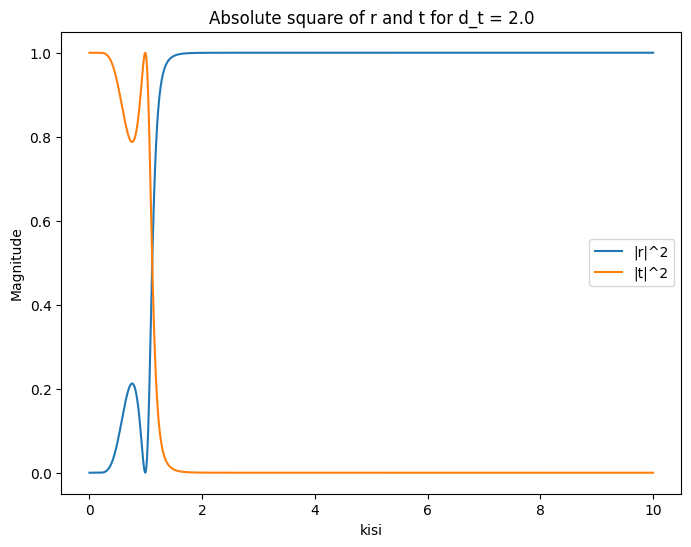
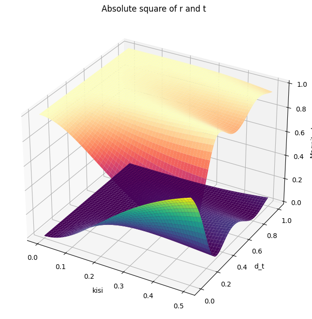
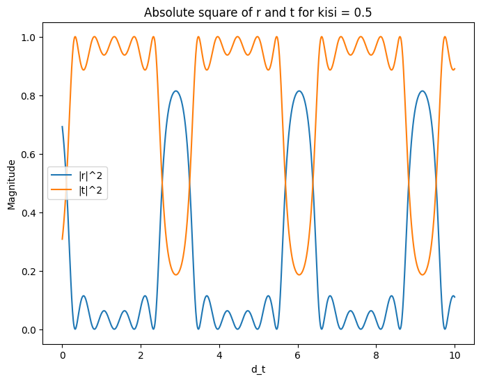
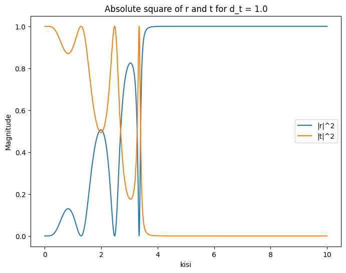
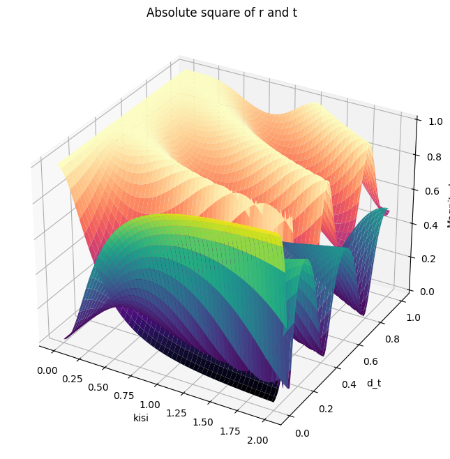
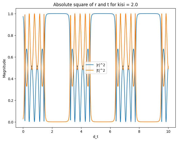
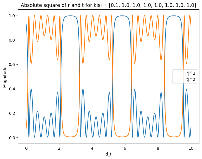
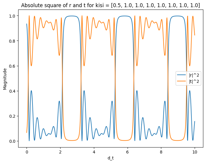
As evident from Figure 4, These graphs illustrate how reflection and transmission probabilities vary with respect to energy and distance. As depicted in the second graph, perfect transmission and reflection can occur multiple times at different energy levels and distances. Additionally, from the last graph, we observe that as the ratio of potential to energy approaches 4, the transmission tends to decrease and approach zero, as anticipated. It is apparent that perfect transmission can occur multiple times. To pinpoint the exact eigenvalue energy for perfect transmission, we achieve this by setting $r=0$ and then determining the value of $\xi$ with respect to varying distances and energy, as outlined in below code:

⬇

d_t,kisi = smp.symbols(’d_t kisi’)

r_value_algebric_eigen = smp.Eq(r_value_algebric, 0)

eigenvalue = smp.solve(r_value_algebric_eigen, kisi)

print(eigenvalue)

For example, let’s explore the concept of perfect transmission in the context of double Dirac delta potentials. In this case, the energy eigenvalue associated with perfect transmission can be expressed as follows

$$\xi=\frac{2}{\tan(d_{t})},$$ (39)

where $d_{t}=kd,\xi=\frac{v}{k},k^{2}=\frac{2mE}{\hbar^{2}}$, this can be applied for any number of potential as well. Now, we examine several cases to observe how the system operates in different situations.

Data visualization and Data analysis for $n=6$, $\tilde{V}=-1$, $d=1$ and $k=1$

Figure 5: Wave functions within a region and the absolute value squared of the wave function when the potential takes the form of a well rather than a barrier.

Figure 6: Plots of transmission and reflection probability in terms of $y$ and $\xi$.

By changing the sign of the potential from a barrier to a well, we can observe the alteration in scattering behavior by comparing the graphs and probabilities with the previous case. As evident in the above graphs, changing the sign of $\xi$ does indeed influence the transmission and reflection probabilities. However, it’s worth noting that the sign of the potential affects the phase shift of these probabilities, as indicated by changes in their distances. In the last graph of Figure 6, we observe that the transmission resonance remains the same.

$$\mid t\mid^{2}=0.23624786700649963,$$ (40)

and

$$\mid r\mid^{2}=0.7637521329935002.$$ (41)

Data visualization and Data analysis for $n=6$, $\tilde{V}=1$, $d=2$ and $k=1$

Figure 7: Plots of wave function and its absolute value squared for $\tilde{V}=1$, $k=1$,$n=6$, $d=2$ and $y_{0}=0$.

Figure 8: Plots of transmission and reflection probability in terms of $y$ and $\xi$.

Increasing the distance can lead to greater oscillation in the particle, as we can predict. From analyzing Figure 7,8 we understand that the number of transmission resonances decreases as the distance increases.

$$\mid t\mid^{2}=0.9965694180598588,$$ (42)

and

$$\mid r\mid^{2}=0.003430581940141181.$$ (43)

Data visualization and Data analysis for $n=6$, $\tilde{V}=1$, $d=1$ and $k=2$

As we increase the energy of the particle, we expect the transmission probabilities to increase, It is apparent from Figures 9 and 10 that as the energy of the particle increases, the probabilities of transmission increase, while the probabilities of reflection decrease.

Figure 9: Plots of the wave function and its absolute value squared for $n=6$, $\tilde{V}=1$, $d=1$ and $k=2$

Figure 10: Plots of transmission and reflection probability in terms of $y$ and $\xi$.

$$\mid t\mid^{2}=0.9460278861581828,$$ (44)

and

$$\mid r\mid^{2}=0.05397211384181813.$$ (45)

Data visualization and Data analysis for $n=6$, $\tilde{V}=2$, $d=1$ and $k=1$

Figure 11: Plots of the wave function and its absolute value squared for $\tilde{V}=2$, $d=1$ and $k=1$

Figure 12: Plots of transmission and reflection probability in terms of $y$ and $\xi$.

From figures 11 and 12 as the strength of the potentials increases, the probabilities of transmission decrease, while the probabilities of reflection increase.

$$\mid t\mid^{2}=0.49395609650026445,$$ (46)

and

$$\mid r\mid^{2}=0.5060439034997339.$$ (47)

III.4.2 Equal distances and Non-equal potentials

Through code modification as shown below, we can introduce impurities in the potential strengths, enabling the exploration of a system. By considering these impurities, we have the opportunity to plot the wave functions, their absolute values squared, as well as the transmission and reflection probabilities. This approach allows for a comprehensive analysis of the system’s behavior under the existence of impurities. The code modification is identical to the previous version; however, it’s important to take caution when defining the range of distances which we can see as follows:

⬇

elif potential_types == ’non equal potentials’and distance_types == ’equal distances’:

lambdified_psi_y_functions = [lambdify(y, func) for func in substituted_psi_y]

l = num_potential-1 # Define the value of n

range_of_graph = [] # Initialize an empty list to store the ranges

start = y0_n - (10 * value_of_distance)

end = y0_n

range_of_graph.append((start, end)) # Add the first range

for i in range(l):

start = y0_n + (i * value_of_distance)

end = y0_n + ((i+1) * value_of_distance)

range_of_graph.append((start, end))

end = y0_n + ((l + 10) * value_of_distance)

range_of_graph.append((y0_n + (l * value_of_distance), end)) # Add the last range

print(range_of_graph)

plt.figure(1)

for i, func in enumerate(lambdified_psi_y_functions):

y_vals = np.linspace(range_of_graph[i][0], range_of_graph[i][1], 1000)

f_vals = np.real(func(y_vals))

plt.plot(y_vals, f_vals, label=str(substituted_psi_y [i]))

plt.xlabel(’y’)

plt.ylabel(’psi_y’)

plt.title(’Plot of wave function’)

lambdified_abs_psi_y_square = [lambdify(y, func) for func in abs_psi_y_square]

m = num_potential - 1

range_of_graph1 = []

start1 = y0_n - (10 * value_of_distance)

end1 = y0_n

range_of_graph1.append((start1, end1))

for i in range(m):

start1 = y0_n + (i * value_of_distance)

end1 = y0_n + ((i + 1) * value_of_distance)

range_of_graph1.append((start1, end1))

end1 = y0_n + ((m + 10) * value_of_distance)

range_of_graph1.append((y0_n + (m * value_of_distance), end1))

plt.figure(2)

for i, func in enumerate(lambdified_abs_psi_y_square):

y_vals1 = np.linspace(range_of_graph1[i][0], range_of_graph1[i][1], 1000)

f_vals1 = np.vectorize(func)(y_vals1)

plt.plot(y_vals1, np.real(f_vals1), label=str(abs_psi_y_square[i]))

plt.xlabel(’y’)

plt.ylabel(’psi_y_square’)

plt.title(’Plot of abs wave function square’)

plt.grid(True)

plt.show()

system_of_equations_algebric = [Eq(eq, 0) for eq in (bc_eq1_n + bc_eq2_n)]

system_of_equations_algebric1 = [eq.subs({symbol: value for symbol, value in zip(kisi_list, kisi_f)}) for eq in system_of_equations_algebric]

symbols_list_algebric = list(set().union(*[eq.free_symbols for eq in system_of_equations_algebric1]))

solution_algebric = smp.solve(system_of_equations_algebric1, symbols_list)

symbol_values_algebric = {symbol: value for symbol, value in solution_algebric.items()}

print(symbol_values_algebric)

r_value_algebric = symbol_values_algebric[r]

t_value_algebric = symbol_values_algebric[t]

r_func = lambdify((d_t), r_value_algebric, modules=’numpy’)

t_func = lambdify((d_t), t_value_algebric, modules=’numpy’)

d_t_values2=np.linspace(0,10,1000)

# Calculate the absolute square of r and t for the fixed kisi

abs_r_product_kisi_list = np.abs(r_func(d_t_values2) * np.conj(r_func(d_t_values2)))

abs_t_square_kisi_list = np.abs(t_func(d_t_values2) * np.conj(t_func(d_t_values2)))

# Plot the 2D graph for the fixed kisi

fig, ax = plt.subplots(figsize=(8, 6))

ax.plot(d_t_values2, abs_r_product_kisi_list, label=’|r|^2’)

ax.plot(d_t_values2, abs_t_square_kisi_list, label=’|t|^2’)

ax.set_xlabel(’d_t’)

ax.set_ylabel(’Magnitude’)

ax.set_title(’Absolute square of r and t for kisi = {}’.format(kisi_f))

ax.legend()

plt.show()

In the subsequent instances, we will examine specific examples of these impurities, considering various scenarios to explore the effects on the system. These examples will help us gain a deeper understanding of the implications of different impurity configurations on the wave functions, absolute values squared, and transmission and reflection probabilities within the system

Data visualization and Data analysis for $n=8$, $\tilde{V_{1}}=0.1$, $\tilde{V_{2}}=\tilde{V_{3}}=\tilde{V_{4}}=\tilde{V_{5}}=\tilde{V_{6}}=\tilde{V_{7}}=\tilde{V_{8}}=1$, $d=1$ and $k=1$

Figure 13: Plots of absolute value squared of wave function and transmission, reflection probabilities in terms of $y$ and $\xi$.

When we take impurities into account, we can illustrate from figure 13 that if the potential strength of the impurity is sufficiently small, we can readily disregard the influence of this potential, as expected.

$$\mid t\mid^{2}=0.9034048285561366,$$ (48)

and

$$\mid r\mid^{2}=0.0965951714438628.$$ (49)

Data visualization and Data analysis for $n=8$, $\tilde{V_{1}}=0.5$, $\tilde{V_{2}}=\tilde{V_{3}}=\tilde{V_{4}}=\tilde{V_{5}}=\tilde{V_{6}}=\tilde{V_{7}}=\tilde{V_{8}}=1$, $d=1$ and $k=1$

By increasing the value of the impurity in the system, the probabilities of transmission and reflection exhibit distinct differences compared to previous cases as shown in figure 14. The greater the magnitude of the impurity, the more significantly the probabilities diverge, highlighting the increased impact of impurities on these probabilities.

Figure 14: Plots of absolute value squared of wave function and transmission, reflection probabilities in terms of $y$ and $\xi$.

$$\mid t\mid^{2}=0.9023078385619591,$$ (50)

and

$$\mid r\mid^{2}=0.09769216143804135.$$ (51)

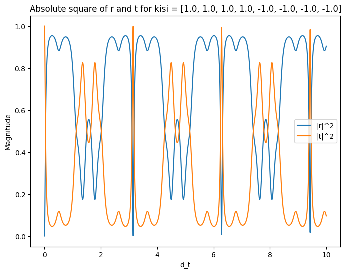
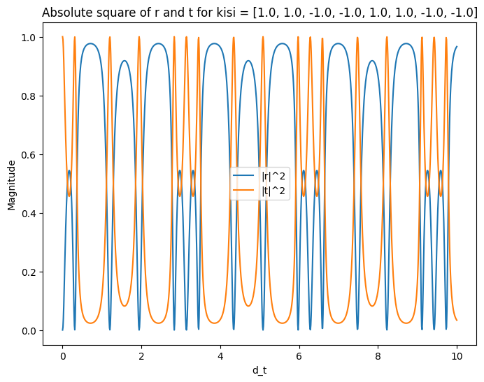
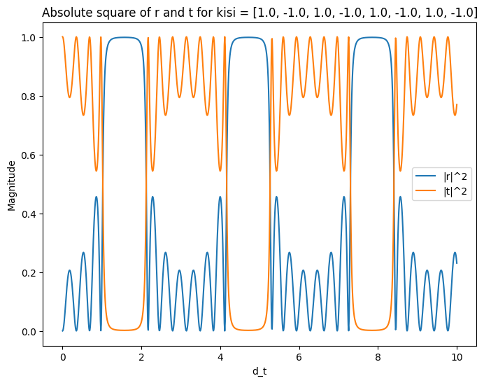
Another interesting point to note is that in a system consisting of multiple Dirac delta potentials with different values, the order or placement of these potentials can indeed cause changes in the probabilities of transmission and reflection. For instance, in a system comprising eight potentials, with four being wells and the remaining four barriers, all with a strength of 1, the placement of these potentials can significantly impact the results of scattering, as demonstrated in the graphs below.

Figure 15: As we can deduce from the aforementioned graphs, the order in which potentials are placed in the system can also have an impact on the transmission and reflection probabilities. An interesting observation from the last graph is that the transmission and reflection probabilities are identical to the case in which all potentials are set to 1.

III.4.3 Non-equal distances and Non-equal potentials

In this section, we extend the generality of our system by further modifying the code. We consider scenarios where distances and potentials are not constrained to be equal. By relaxing these constraints, we explore a more diverse range of possibilities within the system. Despite these variations, we are still able to calculate the transmission and reflection coefficients, allowing us to gain a comprehensive understanding of the system’s behavior under more general conditions.

⬇

else:

system_of_equations_algebric = [Eq(eq, 0) for eq in (bc_eq1_n + bc_eq2_n)]

symbols_list_algebric = list(set().union(*[eq.free_symbols for eq in system_of_equations_algebric]))

solution_algebric = smp.solve(system_of_equations_algebric, symbols_list)

symbol_values_algebric = {symbol: value for symbol, value in solution_algebric.items()}

print(symbol_values_algebric)

r_value_algebric = symbol_values_algebric[r]

t_value_algebric = symbol_values_algebric[t]

Now let’s consider some examples for this specific case imagine we consider a system of 3 potentials with the strength of $\tilde{V_{1}}=1,\tilde{V_{2}}=2,\tilde{V_{3}}=3$ and $d_{1}=1$, $d_{2}=2$ and $k=1$ the coefficient of transmission and reflection are as followed:

$$r=0.44765413320866-0.799041236786126i,$$ (52)

and

$$t=-0.305274111412524+0.260665678288869i.$$ (53)

On the other hand, the analytic solutions for the transmission and reflection coefficients are as follows:

$$t=\frac{-8i}{\gamma+\omega},$$ (54)

$$r=\frac{\lambda+\beta}{\gamma+\omega},$$ (55)

$$\gamma=\xi_{1}\xi_{2}\xi_{3}(e^{2i(d_{1}+d_{2})}-e^{2id_{1}}-e^{2id_{2}}+1)+2i\xi_{1}\xi_{2}(1-e^{2id_{1}}),$$ (56)

$$\lambda=2i\xi_{2}\xi_{3}(e^{2i(d_{1}+d_{2})}-e^{2id_{1}})+4(\xi_{1}+\xi_{2}e^{2id_{1}}+\xi_{3}e^{2i(d_{1}+d_{2})}),$$ (57)

$$\beta=\xi_{1}\xi_{2}\xi_{3}(e^{2id_{1}}+e^{2id_{2}}-e^{2i(d_{1}+d_{2})}-1)+2i\xi_{1}\xi_{2}(e^{2id_{1}}-1)+2i\xi_{1}\xi_{3}(e^{2i(d_{1}+d_{2})}-1),$$ (58)

and

$$\omega=2i\xi_{1}\xi_{3}(1-e^{2i(d_{1}+d_{2})})+2i\xi_{2}\xi_{3}(1-e^{2id_{2}})-4(\xi_{1}+\xi_{2}+\xi_{3})-8i.$$ (59)

Moreover, we find for $\tilde{V_{1}}=1,\tilde{V_{2}}=-2,$ and $d_{1}=1$ and $k=2$

$$r=0.288273992003145+0.45235738801617i,$$ (60)

and

$$t=0.838355921597081-0.0971094627977539i.$$ (61)

Also, the general analytical solutions for the transmission and reflection coefficients for a double Dirac delta potential are as follows.

$$t=\frac{4}{\xi_{1}\xi_{2}(e^{2id_{1}}-1)-2i(\xi_{1}+\xi_{2})+4},$$ (62)

and

$$r=\frac{\xi_{1}\xi_{2}(1-e^{2id_{1}})+2i(\xi_{1}+\xi_{2}e^{2id_{1}})}{\xi_{1}\xi_{2}(e^{2id_{1}}-1)-2i(\xi_{1}+\xi_{2})+4}.$$ (63)

The code allows users to input a wide range of variational values, enabling the simulation of diverse scenarios with any desired number of potentials.

IV conclusion

In this study, we embarked on an exploration of the one-dimensional form of multiple Dirac delta potentials. Utilizing Python programming, we were able to design a quantum system consisting of multiple Dirac delta potentials and investigate quantum scattering in various scenarios. The program provided both numerical and analytical solutions for the transmission and reflection probabilities, accommodating any number of potentials. It also simulated the wave function, providing a comprehensive view of scattering phenomena through graphical representations that revealed the intricate behavior of the system. Furthermore, the program delved into the investigation of transmission resonances, offering exact eigenvalues for the particle’s energy associated with perfect transmission. Moreover, by modifying the code, the program explored the impact of impurities in the scattering process. This research and the associated program contribute to our understanding of quantum scattering and provide a valuable tool for studying the behavior of quantum systems involving multiple Dirac delta potentials in a wide range of scenarios In conclusion, our paper represents a significant contribution to the study of scattering phenomena in quantum mechanics, particularly in the context of impurities in one-dimensional systems with multiple delta Dirac potentials. The development of the Python-based user interface program further enhances the accessibility and accuracy of analyzing and visualizing such systems. As we progress in our understanding of quantum mechanics, the knowledge gained from this research paves the way for future advancements and applications in various scientific and technological domains.

References

- (1) R. de L. Kronig and W. G. Penney, A Quantum Mechanics of Electrons in Crystal Lattices, Proc. R. Soc. 130, 499 (1931).
- (2) C. J. Pethick and H. Smith, Bose-Einstein Condensation in Dilute Gases Cambridge University Press, Cambridge, (2008).
- (3) M. Belloni and R. W. Robinett, The infinite well and Dirac delta function potentials as pedagogical, mathematical and physical models in quantum mechanics, Phys. Rep. 540, 25 (2014).
- (4) Yu N. Demkov and V. N. Ostrovskii, Zero-range Potentials and Their Applications in Atomic Physics, Plenum Press, New York, (1988).
- (5) B. Sahu and B. Sahu,Accurate delta potential approximation for a coordinate-dependent potential and its analytical solution Phys. Lett. A. 373 4033 (2009).
- (6) I. R. Lapidus, Resonance scattering from a double delta-function potential, Am. J. Phys. 50, 663 (1982).
- (7) P. Senn, Threshold anomalies in one dimensional scattering, Am. J. Phys. 56, 916(1988).
- (8) P. R. Berman, Transmission resonances and Bloch states for a periodic array of delta function potentials, Am. J. Phys. 81, 190 (2013).
- (9) G. Cordourier-Maruri, R. De Coss, and V. Gupta, Transmission Properties of the one-dimensional array of delta potentials, Int. J. Mod. Phys. B 25, 1349 (2011).
- (10) ] Z. Ahmed, S. Kumar, M. Sharma, V. Sharma, Revisiting double Dirac delta potential, Eur. J. Phys. 37, 045406 (2016).
- (11) S. H. Patil, Quadrupolar, triple delta-function potential in one dimension, Eur. J. Phys. 30, 629 (2009).
- (12) V. E. Barlette, M. M. Leite, S. K. Adhikari, Integral equations of scattering in one dimension, Am. J. Phys. 69, 1010 (2001).
- (13) D. Lessie and J. Spadaro, One dimensional multiple scattering in quantum mechanics, Am. J. Phys. 54, 909 (1986).