Earthfarseer: Versatile Spatio-Temporal Dynamical Systems Modeling
in One Model

Abstract

Efficiently modeling spatio-temporal (ST) physical processes and observations presents a challenging problem for the deep learning community. Many recent studies have concentrated on meticulously reconciling various advantages, leading to designed models that are neither simple nor practical. To address this issue, this paper presents a systematic study on existing shortcomings faced by off-the-shelf models, including lack of local fidelity, poor prediction performance over long time-steps, low scalability, and inefficiency. To systematically address the aforementioned problems, we propose an EarthFarseer, a concise framework that combines parallel local convolutions and global Fourier-based transformer architectures, enabling dynamically capture the local-global spatial interactions and dependencies. EarthFarseer also incorporates a multi-scale fully convolutional and Fourier architectures to efficiently and effectively capture the temporal evolution. Our proposal demonstrates strong adaptability across various tasks and datasets, with fast convergence and better local fidelity in long time-steps predictions. Extensive experiments and visualizations over eight human society physical and natural physical datasets demonstrates the state-of-the-art performance of EarthFarseer. We release our code at https://github.com/easylearningscores/EarthFarseer.

Introduction

Modeling spatio-temporal (ST) physical dynamics involves estimating states and physical parameters from a sequence of observations (Benacerraf 1973; Newell 1980). Generally, the understanding of a physical process is based on plenty of physical laws, such as Newton’s second law (Pierson 1993) and Conservation of energy law (Sharan et al. 1996; Egan and Mahoney 1972). As tailor-made techniques, dynamical systems, primarily rooted in diverse physical systems, have been demonstrated to conform to most fundamental principles of real-world physical phenomena (Chmiela et al. 2017; Greydanus, Dzamba, and Yosinski 2019), where such phenomena can be mostly recognized by existing mathematical frameworks. To this end, the modeling of dynamic systems has increasingly become a generic approach that yields numerous versatile techniques for various applications. It is crucial in climate science for predicting environmental impacts, in economics and finance for market analysis, in engineering for system design, in public health for disease outbreak modeling, in neuroscience for understanding brain activity, in robotics for AI development, and in logistics for optimizing supply chains. (Hale and Koçak 2012; Humar 2012). Actually, such dynamic systems can naturally model the time-varying evolution including both intricate natural system like meterology dynamics (Wiggins, Wiggins, and Golubitsky 2003; Hale and Koçak 2012; Humar 2012; Harish and Kumar 2016) and complex society system of human mobility like traffic evolutions (Ji et al. 2022; Chen et al. 2022a).

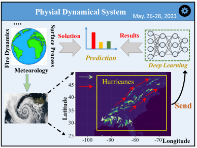
Figure 1: A natural phenomenon in which global and local evolution are inconsistent. The hurricanes primarily exhibit clockwise rotation while in certain localized areas, the presence of convection results in the emergence of counterclockwise rotation.

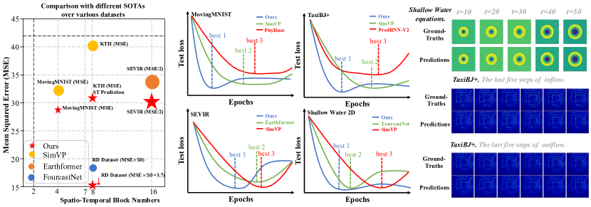
Figure 2: Left. We showcase the performance comparisons between our model and SOTA models across diverse domains. Middle. Convergence of our model compared to other models across different datasets. Right. Our model demonstrates exceptional capability in addressing long-time steps prediction problems.

Since dynamical systems are intrinsically tied to physical processes, they theoretically adhere to the constraints imposed by partial differential equations (PDEs). However, modeling and figuring out the above-mentioned dynamics with inherent physical theories is complicated and intractable to resolve. Fortunately, due to the similar properties of both spatial dependencies and temporal evolution between a general physical process and spatio-temporal modeling, we can opportunely attribute the physical process to a spatio-temporal representation learning problem (Yang et al. 2022; Pathak et al. 2022).

Intriguingly, the fascination of machine learning with physical phenomena has significantly intensified in recent years (Shi et al. 2015; Greydanus, Dzamba, and Yosinski 2019). Many research efforts have turned to video understanding (Chang et al. 2021; Gao et al. 2022b) and physical-guided (Jia et al. 2021; Lu et al. 2021) deep learning to capture ST characteristics in a data-driven manner. These approaches usually design various spatial or temporal components tailored for effectively characterizing a specific scenario or a dedicated task. Although many ST frameworks deliver higher accuracy than the simple ones, they inevitably suffer from partial drawbacks ($\cal D$) outlined below:

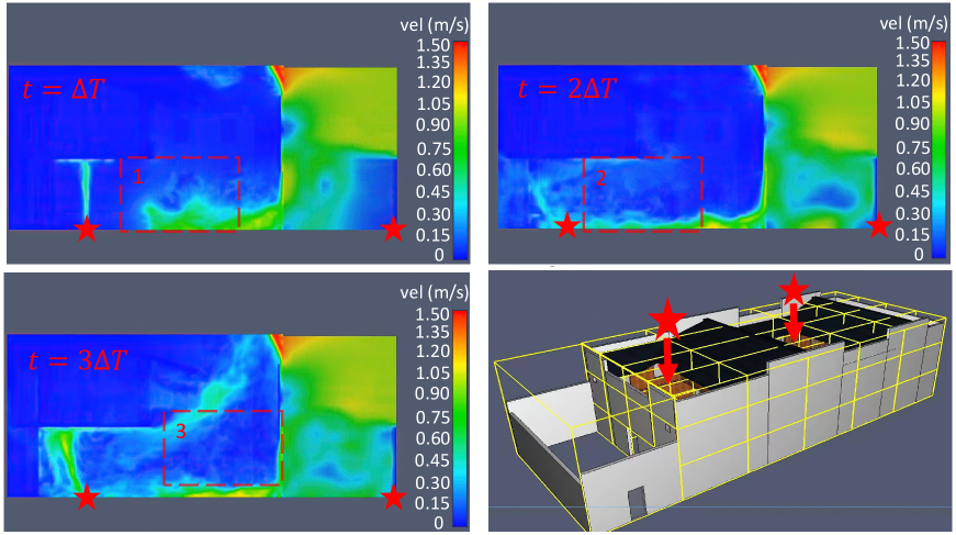
Figure 8: Motivation of our proposal.

• Lack of local fidelity. Given the inconsistency and distinctive local-global dependencies in dynamic systems, existing modules usually focus on global regularity but fail to preserve the local fidelity – local dynamics may differ from global dynamics (See example in Fig 1 and Fig 8 in Appendix A).

• Poor predictions over long time-steps. Complex and continuous dynamic systems often exhibit intricate temporal correlations, leading to poor performance in long-term predictions (Isomura and Toyoizumi 2021).

• Low scalability. The intricate and convoluted component designs confine the model only capable to resolve specific tasks (e.g., super-resolution (Liang et al. 2019), flow prediction (Pan et al. 2019b)) or datasets, leading to limited scalability.

• Inefficiency. The well-designed but cumbersome ST blocks not only contribute to the inefficient training (Wang et al. 2023a, 2022a) process but also pose challenges to the model deployment.

Consequently, the resultant models were neither simple nor practical. Worse still, simultaneously overcoming the aforementioned problems provides an obvious obstacle for existing models. This paper carefully examines and explores the initial systematic study on the aforementioned questions. We introduce a ST framework called EarthFarseer, which is unfolded through the design a universal and Fourier-based ST disentanglement solver, which is different from methods that utilize Fourier operators exclusively in either the spatial or temporal domain (Guibas et al. 2021a). The model overview and contributions are outlined as below:

To highlight, our model exhibits strong adaptability to a wide range of tasks, as well as different datasets encompassing natural physical and social dynamical systems. We place significant emphasis on the fact that our model showcases consistent and reliable results across diverse datasets through simple size scaling, thereby highlighting the inherent scalability of our approach (left side of Fig 2).

For spatial correlations, we employ a parallel local convolution architecture and a global Fourier-based transformer (FoTF) to extract both local and global information. Subsequently, we perform both down-sampling and up-sampling to facilitate effective global-local information interaction and enhance the local fidelity. In our implementation, the fast Fourier transform (FFT) is exploited to transform the patchified two-dimensional outputs from temporal to frequency domain. Each frequency corresponds to a set of tensor values in the spatial domain, so we can quickly perform global perception. This guarantees an efficient model convergence (evidence illustrated in the middle of Fig 2).

For temporal correlations, we design a temporal dynamic evolution module, TeDev, which effectively captures the continuous dynamic evolution within low-dimension space. In comparison to traditional modeling of discrete static frames (Walker, Razavi, and Oord 2021; Wang et al. 2022c), our model undergoes a transformation from the continuous time domain to the frequency domain through Fourier transformation, better preserving the long-term dependence of spatio-temporal data. Further, different from the prevailing neural ordinary differential equation (ODE) algorithms (Park et al. 2021), our model showcases the great prominence in efficiency and long-term prediction tasks when captures intricated dynamics of systems without differential equation based nonlinear features. Through the exploitation of a low-parameter linear convolution projection, TeDev can effciently and accurately predict arbitrary future frames (right side of Fig 2).

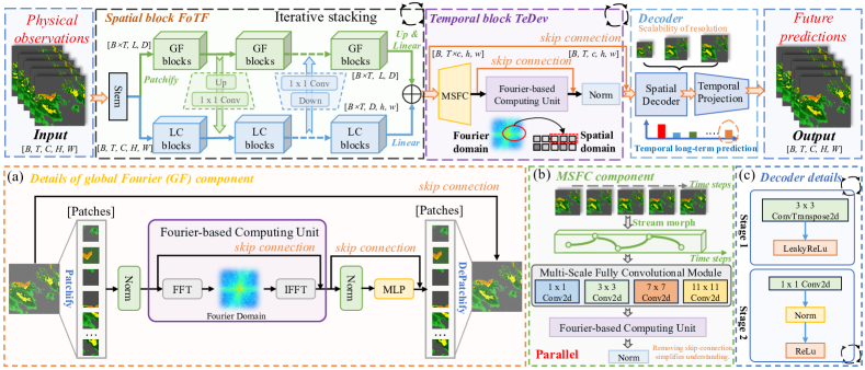
Figure 3: The upper half of the image presents an overview of the model, where Fig (a), (b), and (c) respectively showcase the details of the spatial module, temporal module, and decoding module.

Related Work

Our work shares common ground with several lines of research, and we will now summarize these studies below.

Spatio-temporal prediction methods can be roughly divided into CNN-based (Oh et al. 2015; Mathieu, Couprie, and LeCun 2015; Tulyakov et al. 2018), RNN-based (Wang et al. 2023b, 2022c), and other models including the combinations (Weissenborn, Täckström, and Uszkoreit 2019; Kumar et al. 2019) and transformer based models (Dosovitskiy et al. 2020; Bai et al. 2022). While there are several existing models based on graph neural networks (GNNs), their primary focus is on handling graph data (Wang, Cao, and Philip 2020; Wang et al. 2022b), which go out of the scope of our work.

Video Prediction has become a crucial research topic in the multimedia community, resulting in the proposal of numerous methods to tackle this challenge. Early studies primarily focused on analyzing spatio-temporal signals extracted from RGB frames (Shi et al. 2015). Recently, there has been a growing interest in integrating video prediction with external information such as optical flow, semantic maps, and human posture data (Liu et al. 2017; Pan et al. 2019a). However, in real-world applications, accessing such external information may not always be feasible (Wu et al. 2023; Anonymous 2023). Moreover, the current solutions still exhibit suboptimal efficiency and effectiveness when dealing with high-resolution videos. In this study, we concentrate on modeling continuous physical observations, which can sometimes be interpreted as a video prediction task.

Methodology

As depicted in Fig 3, EarthFarseer comprises three primary components: the FoTF spatial module, the TeDev temporal module, and a decoder. Going beyond ST components, we highlight decoder ability to handle spatial scale expansion and arbitrary length prediction in the temporal domain. we will present the preliminaries and elaborate on the contributions of each of our modules towards achieving local fidelity, model scalability, and SOTA performances.

Preliminaries

The dynamical systems dictate the principles that govern the transition of the current system state to its future continuous state. Formally, given an environment space $X$ and a state space $S\subset X$, a dynamical system can be represented by a function $F$:

$$\bm{X}_{t+\mathrm{d}t}=F\left(\bm{X}_{t}\right),\quad t=0,dt,2dt,3dt,\ldots$$ (1)

where $X_{t}\in S$ is the system’s current state at time t, which can be further understood as a snapshot. Each snapshot contains $C$ color channels within a spatial resolution of $H\times W$. $dt$ represents the time increment. $F:S\rightarrow S$ describes the state evolution of the system from $X_{t}$ to its successive state $X_{t+dt}$. We consider the discrete time system, as any time-continuous system can be discretized with an appropriate $dt$.

Spatial block FoTF

FoTF contains two branches, namely, the local CNN module (LC block) and the global Fourier-based Transformer (GF), which work in parallel to enhance global perception and local fidelity. We model continuous physical observations as image inputs with a batch size of $B$ and a time length of $T$. Then, the input dimension is $[B,T,C,H,W]$ and we feed inputs into a Stem module, which includes a 1x1 successive convolution for initial information extraction.

Local CNN Branch

utilizes a CNN architecture to capture fine-grained features. Due to the strong inductive bias of CNNs, we employ smaller convolutional kernels, i,e,, 3x3, to enable the model with local perceptual capabilities. Specifically, LC is composed of $N_{e}$ ConvNormRelu unit:

$$\begin{gathered}{\rm{Z}}_{LC}^{i+1}={\rm{LeakyRelu}}({{\rm{GNorm}}({{\rm{Conv}2{\rm{d}}}({{\rm{Z}}_{LC}^{i}})})})\in\mathbb{R}^{[B\times T,D,h,w]},\\ 1\leq i\leq N_{e}\end{gathered}$$ (2)

where $\rm{GNorm}$ and $\rm{LeakyRelu}$ denote group normalization and leaky relu function, respectively. ${\rm{Z}}_{LC}^{j+1}$ denotes output from $j$-th LC block. Generally, LC block maps high-dimensional inputs into relatively low-dimensional representations ($H>h,W>w$), which will then be sent to temporal evolution module.

Global Fourier-based Transformer

runs in parallel with the CNN branch, and in each stage, the size of the Transformer feature is consistent with the LC output feature. Let $X_{t}\in\mathbb{R}^{H\times W\times C}$ be an input observation at time $t$, the image is first tokenized into $L=HW/{p^{2}}$ non-overlapping patches with $p\times p$ patch size. Each patch is projected to an embedding $z\in\mathbb{R}^{D}$ by adopting a linear layer. Then we can obtain the tokenized image:

$$Z_{t}=(z_{t}^{1};\ldots;z_{t}^{L})\in\mathbb{R}^{L\times D}$$ (3)

where (; …; ) denotes row-wise stacking. For better understanding, we remove the subscript ”t” to illustrate subsequent operations. To accommodate multiple batches and time steps inputs, we patchify them into dimensions, i.e., $[B\times T,L,D]$ compatible with the Transformer architecture as depicted above. Inspired by (Guibas et al. 2021b), we replace multi-head self-attention (MSA) based token mixing with Fourier-based token mixing operator. Fourier transform converts an image from the spatial to the spectral domain, where each frequency corresponds to a set of spatial pixels. Therefore, the Fourier filter can process an image globally, rather than targeting a specific part like LC blocks. We conduct 2D real-valued fast Fourier transform (FFT) on patchified embedding ${\hat{Z}_{GF}}$:

$${\cal F}({\hat{Z}_{GF}})=\mathcal{F}[\hat{Z}_{GF}(x)]=\int_{-\infty}^{\infty}\hat{Z}_{GF}(x)e^{-2\pi ikx}dx$$ (4)

where $k$ represents frequency, and $x$ represents the position within the spectral sequence, ${\hat{Z}_{GF}}$ is updated to its spectral domain representation with FFT. Similar to (Huang et al. 2023), we take advantage of the conjugate symmetric property of the discrete Fourier transform and retain only half of the values for efficiency. After the Fourier transformation, we apply a linear transformation using a MLP. The purpose of this linear transformation is to map the frequency domain representation into a linear space, ensuring that the output has the same dimensionality as the input:

$${\cal F}({\hat{Z}_{GF}})\leftarrow{\rm MLP}({\cal F}({\hat{Z}_{GF}}))$$ (5)

We replace MSA with MLP, which can significantly reduce the computational complexity from $N^{2}d+3Nd^{2}$ to quasi-linear $Nd^{2}/k+Nd\log N$. Here $N$ refers to the sequence size (equal to the product of the height ($h$) and width ($w$) of the spatial grid.) and parameter $d$ represents the channel size. Here $m$ corresponds to the number of blocks used in GF component. The outputs from the MLP are then sent to an Inverse FFT (IFFT) module:

$${\hat{Z}_{GF}(x)}={\mathcal{F}^{-1}}_{k}[F(k)](x)=\int_{-\infty}^{\infty}F^{+}(k)e^{2\pi ikx}dk$$ (6)

In this context, $\hat{Z}_{GF}(x)$ represents the output obtained after the IFFT, $F^{+}(k)$ denotes the result of the linear transformation. The primary objective of GF model is to transform the input in the spectral domain, map it to an output of the same dimensionality, and then revert it back to the time domain through the IFFT. This modul demonstrate the capability to effectively approximate global, long-range dependencies in higher resolution signals, all while avoiding the need for excessively deep architectures. We place model implement details in Appendix E.

Global-local interactions.

We iteratively interact global GF and local LC modules multiple times to achieve information fusion. Concretely, we employ conv2d layer for upsampling (Up) and transposeconv2d for downsampling (Down), both with a kernel size of 3, stride of 1, and maintaining the same dimensions (The upper half of Fig 3). In the final spatial block, we upsample the last GF output (with dimensions $[B\times T,L,D]$) and map it to the dimensions of $[B,T\times c,h,w]$ using a linear layer.

Temporal block TeDev

As shown in Fig 3(b), stream morph operator first converts the discrete ST sequence into a continuous stream, followed by the MSFC module and the Fourier-based computational unit to complete the hidden feature extraction. Stream morph combines the channel dimension and the time dimension, enabling the transformation of discrete temporal dynamics into a continuous and irregular representation. The MSFC module stands out from traditional methods by utilizing a multi-scale fully convolutional (MSFC) architecture with various kernel sizes. This architecture enables feature extraction from a global to local perspective, with larger kernel sizes (7 and 11) capturing global information distribution and smaller sizes (1 and 3) facilitating locality. TeDev also integrates FFT/IFFT module, which converts time-domain signals into frequency-domain signals (See Eq $4\sim 6$), facilitating a better understanding and analysis of signal components. As a result, TeDev captures information at different time scales and avoids losing temporal information during spatiotemporal prediction. Formally, TeDev can be described as follows:

$$\begin{gathered}z^{j+1}=\sum_{k\in\{1,3,7,11\}}\operatorname{Conv2d}_{k\times k}\left(\operatorname{Conv2d}_{1\times 1}\left(h^{j}\right)\right),\\ z^{j+1}=\mathcal{F}^{-1}{\rm(MLP(\mathcal{F}(z^{j+1})))}\in\mathbb{R}^{[B,T,c,h,w]},N_{e}\leq j\leq N_{e}+N_{t}\end{gathered}$$ (7)

$N_{t}$ temporal blocks take the encoded hidden representation $z^{j}$ of the spatial encoder as input and obtain the hidden feature $z^{j+1}$ for the next time step. The feature is then processed by FFT/IFFT transform. In summary, TeDev’s temporal evolution module comprehensively acquires features across scales from a continuously evolving time stack. It combines the output features of convolutional layers with diverse kernel sizes and performs spectral operations to ensure dimensional consistency.

Decoder

Our decoder consists of two stages, i.e., spatial and temporal decoders, which allows for adaptation to different resolutions and flexible future time-step predictions.

Spatial Decoder

employs $N_{d}$ blocks to effectually reconstruct the latent features into an output of the desired size, which may assume any resolution. To be specific, it employs ConvTranspose2d for upsampling the encoded features to the target resolution, followed by the utilization of Tanh as the activation function to obtain the output. The layer combination form is explicated as follows:

$$\begin{gathered}z^{d+1}={\rm{Tanh}}(\operatorname{ConvTranspose2d}(z^{d}))\in\mathbb{R}^{[B,T,C,H,W]},\\ N_{e}+N_{t}<d\leq N_{e}+N_{t}+N_{d}\end{gathered}$$ (8)

Temporal Projection

In order to flexibly predict future lengths, we utilize the ConvNormRelu unit to expand the time channel. Specifically, we concatenate the time and channel dimensions of the decoded features $z^{d+1}\in\mathbb{R}^{[B,T,C,H,W]}$ obtained in the first stage, resulting in a tensor of size $T\times C$, which is then mapped to $K\times C$, where $K$ is the desired target length, which can theoretically be any value. Subsequently, we perform a dimensional transformation on the resulting feature map to obtain the predicted target dimension $z^{d+2}\in\mathbb{R}^{[B,K,C,H,W]}$. The formal calculation process is as follows:

$$\begin{gathered}{z}^{d+2}={\rm{Relu}}({{\rm{Norm}}({{\rm{Conv}2{\rm{d}}}({{z}^{d+1}})})})\in\mathbb{R}^{[B,K,C,H,W]}\end{gathered}$$ (9)

Through the aforementioned spatio-temporal decoding module, we can output the results to specific resolutions and durations according to the requirements of specific prediction tasks, thus accommodating a wider range of needs.

Table 1: Dataset statistics. $N\_tr$ and $N\_te$ denote the number of instances in the training and test sets. The lengths of the input and prediction sequences are $I_{l}$ and $O_{l}$, respectively.

Dataset	$N\_tr$	$N\_te$	($C,H,W$)	$I_{l}$	$O_{l}$	Interval
MovingMNIST	9000	1000	(1, 64, 64)	10	10	–
TaxiBJ+	3555	445	(2, 128, 128)	12	12	30 mins
KTH	108717	4086	(1, 128, 128)	10	20	–
SEVIR	4158	500	(1, 384, 384)	10	10	5 mins
RainNet	6000	1500	(1, 208, 333)	10	10	1 hour
PD	2000	500	(3, 128, 128)	6	6	5 seconds
RD	2000	500	(3, 128, 128)	2	2	1 second
2DSWE	4000	1000	(1, 128, 128)	50	50	–

Experiments

Table 2: Model comparison with the state-of-the-arts over different evaluation metrics. We report the mean results from three runs. Given the distinct characteristics of various datasets, we present different dimensions across different rows to account for their unique properties.

Datasets	Metrics	Models
		ConvLSTM	PredRNN-v2	E3D-LSTM	SimVP	VIT	SwinT	Rainformer	Earthformer	PhyDnet	Vid-ODE	PDE-STD	FourcastNet	Ours
	MSE	103.3	56.8	41.3	15.1	62.1	54.4	85.8	41.8	24.4	22.9	23.1	60.3	14.9
MovingMNIST	MAE	182.9	126.1	86.4	49.8	134.9	111.7	189.2	92.8	70.3	69.2	68.2	129.8	33.2
	MAE	5.5	4.3	4.1	3.0	3.4	3.2	- -	- -	4.2	3.9	3.7	- -	2.1
TaxiBJ+	MAPE	0.621	0.469	0.422	0.307	0.362	0.306	- -	- -	0.459	0.413	0.342	- -	0.243
	MSE	126.2	51.2	86.2	40.9	57.4	52.1	77.3	48.2	66.9	49.8	65.7	102.1	31.8
KTH	MAE	128.3	50.6	85.6	43.4	59.2	55.3	79.3	52.3	68.7	50.1	65.9	104.9	32.9
	MSE	3.8	3.9	4.2	3.4	4.4	4.3	4.0	3.7	4.8	4.5	4.4	4.6	2.8
SEVIR	CSI-M × 100	41.9	40.8	40.4	45.9	37.1	38.2	36.6	44.2	39.4	34.2	36.2	33.1	47.1
	RMSE	0.688	0.636	0.613	0.533	0.472	0.458	0.533	0.444	0.533	0.469	0.463	0.454	0.437
RainNet	MSE	0.472	0.405	0.376	0.284	0.223	0.210	0.284	0.197	0.282	0.220	0.215	0.206	0.191
	MSE	10.9	9.6	10.1	5.4	8.7	8.4	8.6	7.2	6.9	4.8	3.7	5.1	2.2
PD	MAE	100.3	95.4	100.2	50.9	81.2	79.5	80.9	73.4	68.7	47.6	38.9	52.4	21.8
	MSE × 10	21.2	20.9	18.2	9.5	13.2	12.1	9.7	11.4	10.8	9.8	9.8	10.2	9.4
RD	MAE	52.7	50.1	42.6	17.8	27.3	25.9	43.2	45.9	22.6	20.7	20.3	21.9	16.8
	MSE × 100	11.2	8.9	6.4	3.1	8.1	7.6	7.8	7.4	4.9	4.5	4.3	5.2	2.6
2DSWE	MAE	54.3	53.1	30.2	17.2	52.7	50.3	51.4	49.2	20.1	19.8	19.5	21.7	10.5
Avg Ranking		6.2	3.5	4.3	3.3	3.3	3.5	5.2	4.7	5.3	4.6	5.2	4.8	1.7

In this section, we empirically demonstrate the superiority of our framework on seven datasets, including two human social dynamics system (TaxiBJ+, KTH (Schuldt, Laptev, and Caputo 2004)), five natural Scene dynamical systems (SEVIR (Veillette, Samsi, and Mattioli 2020), RainNet (Chen et al. 2022b), Pollutant-Diffusion (PD), Reaction-Diffusion) and 2D shallow water Equations (2DSWE) (Takamoto et al. 2022), and a synthetic systems (MovingMNIST (Srivastava, Mansimov, and Salakhudinov 2015)). In the subsequent section, we will provide a detailed introduction to the dataset and baseline, along with the corresponding experimental settings and results.

Experiment setting

Dataset Description.

We conduct extensive experiments on eight datasets, including two human social dynamics system (II, III), five natural scene datasets (IV, V, VI, VII, VIII) and a synthetic datasets (I) in Tab 1, for verifying the generalization ability and effectiveness of our algorithm. See dataset details in Appendix C and D.

Baselines for Comparison.

We compare EarthFarseer with the following baselines that belong to three categories:

• Video Prediction Models: We select ConvLSTM (Shi et al. 2015), PredRNN-v2 (Wang et al. 2022c), E3D-LSTM (Wang et al. 2019) and SimVP-v2 (Tan et al. 2022) as some of the most representative and advanced RNN architecture models in recent years.

• Spatio-temporal Series Modeling: We conduct experiments on advanced Transformer architecture models, including Vision Transformer (Dosovitskiy et al. 2020), Swin Transformer (Liu et al. 2021), Rainformer (Bai et al. 2022) and Earthformer (Gao et al. 2022a).

• Physics-guided Neural Networks: We use modeling methods that incorporate PDE or ODE in the model as baseline models for comparison, including Ad-fusion model, PhyDnet (Guen and Thome 2020), Vid-ODE (Park et al. 2021), PDE-STD (Donà et al. 2020), and FourcastNet (Pathak et al. 2022), and FourcastNet represents a meteorological modeling model in the neural operator field.

Evaluation Metrics. We train our model with mean squared error (MSE) metric. We further use MSE, mean absolute error (MAE), and mean absolute percentage error (MAPE) as common evaluation metrics. Additionally, for the SEVIR dataset, we add the CSI index (Ayzel, Scheffer, and Heistermann 2020) as a core metric for comparison. We place the metrics descriptions in Appendix B.

Implementation Details. We implement our model using PyTorch framework and leverage the four A100-PCIE-40GB as computing support. In our paper, we generate model configurations (ours-$Ti/S/B$) by adjusting ST block numbers equal to 6,12,24. Concretely, tiny ($Ti$), small ($S$) and Base ($B$) models have $6$, $12$ and $24$ ST Blocks, respectively. Specifically, ST block can be divided into three sub-blocks, namely spatial encoder FoTF, temporal block TeDev and decoder block. We have placed the detailed descriptions in table 4 in Appendix C.

Main Results

In this subsection, we thoroughly investigate the scalability and effectiveness of EarthFarseer on various datasets. We conduct a comprehensive comparison of our proposal with video prediction, spatio-temporal series, and physical-guided models, for ST tasks on the social dynamics system, synthetic, and natural scene datasets (Tab 2). We summarize our observations (obs) as follows: Obs 1. EarthFarseer consistently outperforms existing methods under the same experimental settings over all datasets, verifying the superiority of our ST blocks via global-local modeling component and temporal Fourier design. Obs 2. Our model scales well to large datasets and performs well. For instance, on SEVIR dataset (64.83GB with resolution 384×384), we surpass the SOTA (Earthformer) 0.0287 on CSI-M metric, which demonstrates the scalability of our proposal. Obs 3. On certain physical datasets that PDE information, such as 2DSWE, physics-guided models like PDE-STD and FourcastNet outperform primarily video prediction models (except SimVP) and ST models, yielding superior results. Our model adeptly captures the underlying principles of PDEs, exhibiting a lower MAE index ranging from $0.5$ to $5.2$ compared to existing video prediction/PDE-based models.

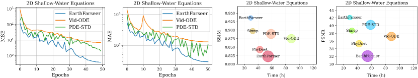
Figure 4: Model performance on 2DSWE dataset with different baselines. We measure the time it takes for the model to reach optimal performance by conducting fair executions across all frameworks on a Tesla V100-40GB.

Model Analysis

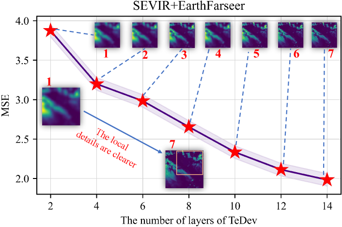
Figure 5: Model performance on SEVIR dataset with different number of temporal layers.

${\cal Q}1$: Scalability analysis. In our implementation, we can quickly expand the model size by stacking blocks layers. As shown in Tab 2, we further explore the scalability of the temporal and spatial module. As meteorological exhibit highly nonlinear and chaotic characteristics, we selected the SEVIR to analyze the scalability of temporal component. We conduct experiments by selecting $2\sim 14$ TeDev blocks layers, under settings with batch size as 16, training epochs as 300, and learning rate as 0.01 (Adam optimizer). The visualization results are presented quantitatively in the Fig 5. With the increase of the number of TeDev Blocks, we can observe a gradual decrease in the MSE index, and we can easily find that loacl details are becoming clearer as time module gradually increases. This phenomenon once again demonstrates the size scalability of our model. Notably, our model incorporates a ViT-like architecture, offering intriguing possibilities for future expansion in a specific context.

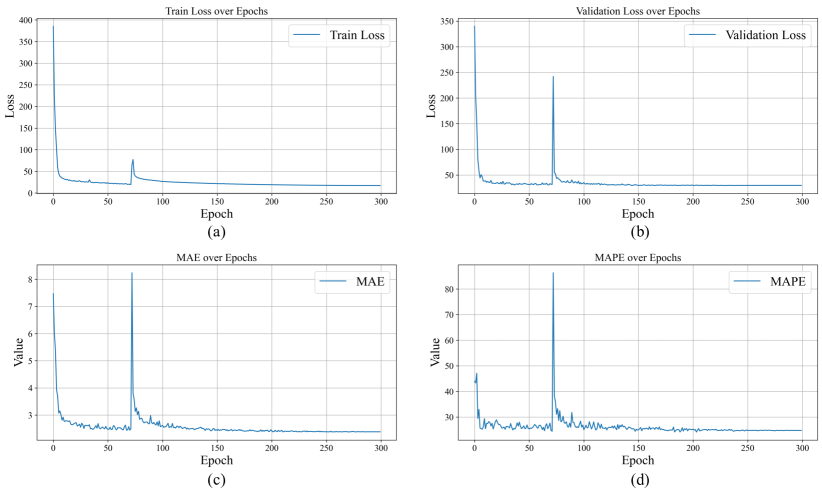
Figure 15: (a). Train Loss over Epochs: This graph illustrates the change in training loss over the training epochs. As the training progresses, the model should gradually adapt to the training data, resulting in a decrease in training loss.(b). Validation Loss over Epochs: This graph shows the change in validation loss over the training epochs. Validation loss is a performance metric for the model on unseen validation data, and it helps in identifying whether the model is overfitting or underfitting.(c). MAE over Epochs: This graph depicts the change in Mean Absolute Error (MAE) over the training epochs. MAE is a measure of the difference between the model’s predictions and the actual values, with a lower MAE indicating more accurate predictions.(d). MAPE over Epochs: This graph illustrates the change in Mean Absolute Percentage Error (MAPE) over the training epochs. MAPE is a measure of the relative difference between the model’s predictions and the actual values, expressed as a percentage. A lower MAPE indicates predictions that are closer to the actual values.

We also conduct super-resolution experiments to further illustrate the scalability issues. In TaxiBJ+, we downsample the training data to $32\times 32$ pixels to forecast future developments at $128\times 128$ pixels over 12 steps. We discovered that the MAE was only 2.28 (MAPE=0.247). Compared to certain non-super-resolution prediction models, our results were significantly superior. This further demonstrates our model’s capability in predicting spatial tasks across different resolutions (Fig 15&16 for the visualization and training).

${\cal Q}2$: Efficiency analysis. Due to the inherent complexity of solving PDEs, we select the 2DSWE dataset with PDE property as the benchmark for validating the efficiency of our model. As shown in Fig 5, we can list observation: Obs 1. EarthFarseer presents a lower training error during the whole training process. Obs 2. Our model can achieve better convergence in faster training time. Specifically, we can save nearly 3/4 of the training time compared to VideoODE, which further verify the efficiency of EarthFarseer.

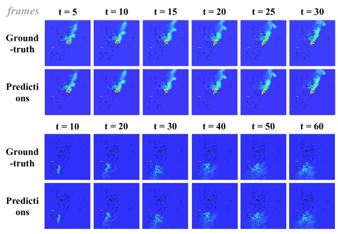
Figure 10: Quantitative performance in experiments involving 10 $\to$ 30 and 10 $\to$ 60 frames on PD datasets.

${\cal Q}3$: Predicting future frames with flexible lengths. EarthFarseer can address the issues of accumulated error and delay effects in RNN-based models for predicting frames of arbitrary length. With a two-stage design, our approach restores the feature map to the input dimension, effectively preserving spatial feature information. Additionally, it utilizes a linear projection layer to expand the time channel, allowing for convenient adjustment of the output frame length. Evaluation on TaxiBJ+, PD and 2DSWE datasets reveals that EarthFarseer exhibits remarkable quantitative performance in experiments involving 10 $\to$ 30, 10 $\to$ 60 and 50 $\to$ 50 frames (Fig 10, 6 and 14). We also showcase the 20 $\to$ 80 frames results on 2DSWE with different backbones, EarthFarseer outperforms baseline models the large margins (Tab 5), highlighting EarthFarseer’s exceptional flexibility and prediction accuracy. These findings position EarthFarseer as a promising method in ST domains.

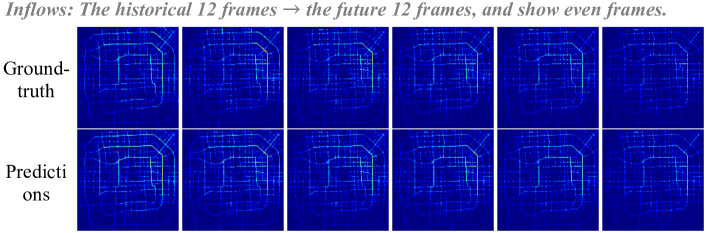
Figure 6: Visualization of inflow and outflow prediction results on the TaxiBJ+ dataset. Aigned with Fig 9 in Appendix D.

${\cal Q}4$: Local fidelity analysis.

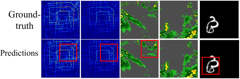
Figure 7: Visualizations of our framework on TaxiBJ+, SEVIR and MovingMNIST datasets, from which we can find that our model can preserve the local fidelity very well.

We proceed to consider another issue, i.e., local fidelity problem. We choose TaxiBJ+, SEVIR and MovingMNIST dataset as validation datasets. As shown in Fig 7, our findings indicate that EarthFarseer effectively maintains local details while preserving the overall global context, particularly in the case of local outliers. This ability allows for the achievement of high fidelity in preserving local information. These results substantiate the local awareness exhibited by our model. For ease of understanding, we present the more complete visualizations in Appendix D (Fig 11 $\sim$ 12).

Ablation Study

In this part, we further explore the effectiveness of each individual component. In our settings, A denotes remove local convolutional component and D represents replace decoder with linear convolutional decoder. As shown in Tab 3, our ablation experiments demonstrate that removing any module from our model leads to varying degrees of performance degradation. Both the local constraint (LC) and global constraint (FoTF) contribute to the model’s performance on the spatial modules. For example, on the TaxiBJ+ dataset, removing the LC module leads to a decrease of 0.7 in the MAE metric, and removing the FoTF module leads to a decrease of 0.3. Our TeDev module outperforms the models using ViT and SwinT as a replacement for TeDev on the MovingMNIST and PD datasets. This suggests that our TeDev module is more suitable for tasks involving temporal information than using Transformer models. In summary, our model exhibits stronger expressive power in all scenarios, demonstrating the effectiveness of our proposal.

Table 3: Results of ablation experiments for different model structures on MovingMNIST, TaxiBJ+, and PD datasets. model effects were evaluated using MSE metrics for MovingMNIST and PD datasets and MAE metrics for TaxiBJ+ dataset.

Method	MovingMNIST	TaxiBJ+	RD
(A) Ours w/o LC	19.7	2.8	14.1
(B) Ours w/o FoTF	16.6	2.4	17.2
(C) Ours w/o TeDev	22.1	3.1	17.8
(D) Ours w/o Decoder	15.9	2.2	10.2
(E) Ours TeDev $\to$ ViT	23.5	3.5	16.2
(F) Ours TeDev $\to$ SwinT	21.3	3.2	14.3
Ours (Full model)	14.9	2.1	9.4

Conclusion

This paper addresses the limitations of existing models that arise from the meticulous reconciliation of various advantages. We conducted a systematic study on the shortcomings faced by such models, including low scalability, inefficiency, poor long output predictions, and lack of local fidelity. We propose a scalable framework that combines spatial local-global information extraction module and temporal dynamic evolution module. EarthFarseer demonstrates strong adaptability across various tasks and datasets, exhibiting fast convergence and high local fidelity in long-distance prediction tasks. Through extensive experiments and visualizations conducted on eight physical datasets, we showcase the SOTA performance of our proposal.

APPENDIX

A. Motivation of our proposal

In this section, we provide an illustrative example of fire evolution to enhance the understanding of both global and local disparities. As shown in Fig 8, two fires (★) broke out in a building and we showcase the global and local speed of fire spread. At a local level, the convection resulting from multiple indoor fire points can generate areas with lower flow rates due to mutual interference. This prevailing phenomenon vividly demonstrates distinct local characteristics within specific spatiotemporal scenes, in stark contrast to the global situation. Consequently, it is crucial to closely monitor these local regions, particularly in emergency scenarios like fires, where knowledge of diminished flow rates can effectively guide crowds and assist firefighters in responding to the crisis with heightened efficiency.

B. Details of the evaluation metrics

One commonly used metric in precipitation forecasting is the Critical Success Index (CSI) (Ayzel, Scheffer, and Heistermann 2020; Gao et al. 2022a), which evaluates the accuracy of the predictions. The formula for CSI is as follows: $\rm{CSI}$ = $\rm{Hits/(Hits+Misses+F.Alarms)}$, where $\rm{Hits}$, $\rm{Misses}$, and $\rm{F.Alarms}$ represent the number of true positives, false negatives, and false positives, respectively. To calculate these numbers, the predicted and actual values are rescaled to a range of 0-255, and binary values are obtained using threshold values [16, 74, 133, 160, 181, 219].

By calculating the CSI values at different threshold levels, we can evaluate the performance of the prediction model and use the average $\rm{CSI}-M$ as an overall evaluation index. A higher $\rm{CSI}$ value indicates that the model accurately predicts precipitation, while a lower $\rm{CSI}$ value means that the model’s prediction ability needs improvement. Therefore, $\rm{CSI}$ is an important evaluation metric in precipitation forecasting, which helps us understand the quality of the prediction model and guides the improvement of the prediction algorithm.

Hits, Misses, and F.Alarms are important indicators for evaluating the performance of the prediction. Specifically:

• True positive ($\rm{Hits}$) represents the model’s correct prediction of the occurrence of precipitation;

• False negative ($\rm{Misses}$) represents the model’s failure to correctly predict the occurrence of precipitation;

• False positive ($\rm{F.Alarms}$) represents the model’s incorrect prediction of the occurrence of precipitation, i.e., predicting precipitation when it does not occur.

The higher the number of $\rm{Hits}$, $\rm{Misses}$, and $\rm{F.Alarms}$, the worse the performance of the prediction model. Therefore, in precipitation forecasting, we aim to increase the number of $\rm{Hits}$ as much as possible, while reducing the number of $\rm{Misses}$ and $\rm{F.Alarms}$, in order to improve the accuracy and reliability of the predictions.

C. Experimental settings

Some details of our experimental setup are shown in the Tab 4.

Table 4: Table of the number of components for models of different sizes. spatial encoder can be summarized as [Fusion(Fourier2d, Conv2d)], temporal encoder can be summarized as [DownConv2d + Fourier2d + UpConv2d], and decoder can be denoted as [DownConv2d + Fourier2d + UpConv2d].

Model size	FoFT	TeDev	Decoders	Dataset default Settings
Tiny ($Ti$)	2	2	2	I, II, VII, VIII
Small ($S$)	4	4	4	III, VI
Base ($B$)	8	8	8	IV, V

D. Additional experiments

We conduct extensive experiments on eight datasets, including two human social dynamics system (II, III), five natural scene datasets (IV, V, VI, VII, VIII) and a synthetic datasets (I), for verifying the generalization ability and effectiveness of our algorithm.

• MovingMNIST: This dataset contains handwritten digits from the MNIST dataset, placed randomly and moving with random velocities.

• TaxiBJ+: The dataset contains trajectory data of Beijing from taxi GPS, with two channels of inflow and outflow, respectively. We also extend the original dataset by collecting the latest trajectory data of Beijing and increasing the resolution from 32$\times$32 to 128$\times$128, named TaxiBJ+.

• KTH: This dataset includes 25 human performing six types of actions: walking, jogging, running, boxing, waving, and clapping. The complexity of human motion arises from the individual variability in performing different actions. By observing previous frames, the model can learn the dynamics of human motion and predict long-term posture changes in the future.

• SEVIR: The SEVIR dataset contains radar-acquired measurements of vertical accumulation liquid (VIL), acquired every 5 minutes with a resolution of 1 km, and is the baseline dataset used for rain and hail detection.

• RainNet: This benchmark contains more than 62,400 pairs of high-quality low/high-resolution precipitation maps for over 17 years, ready to help the evolution of deep learning models in precipitation downscaling.

• Pollutant-Diffusion (PD): This data are obtained from the computational fluid dynamics (CFD) simulation results of pollutant dispersion in a fixed area. We choose wind speed $15m/s$, wind direction due north, centering point as the kinetic data of the source release point.

• Reaction-Diffusion (RD): This dataset describes the temporal and spatial evolution of material concentration in biological and chemical systems. Each image in the dataset can be regarded as a solution of this equation in two-dimensional space.

• 2D Shallow-Water Equations (2DSWE): The Navier-Stokes equation is the basic equation describing viscous flow in fluid mechanics. The shallow water equation can be derived from the Navier-Stokes equation and used to model free surface flow problems.

In this section, we showcase some the additional experimental results to demonstrate the excellent capabilities of our model. Fig 9 demonstrates that our model excels at preserving intricate details on the TaxiBJ+ dataset. Notably, it accurately captures and retains the fine-grained information within the areas labeled A, B, and C. In Fig 11, we showcase the visualizations of our framework on SEVIR, from which we can easily find that EarthFarseer exhibits the capability to capture local details, as indicated by the red boxes. This phenomenon is further corroborated by the observations presented in Fig 12.

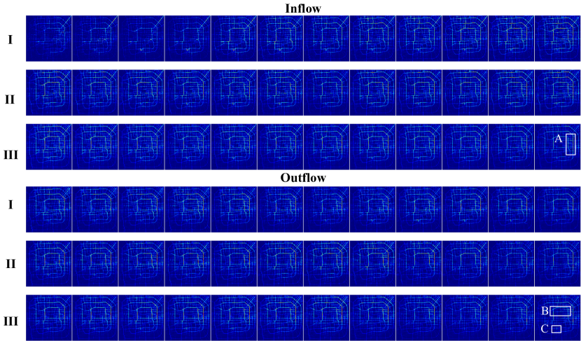
Figure 9: Visualizations of our framework on TaxiBJ+, from which We can find that our model can handle local details very well. I represents the input sequence, II represents the true sequence, and III represents the predicted sequence.

While the majority of datasets in this paper can be obtained from the relevant literature, there are a few newer datasets (Pollutant-Diffusion) that pose challenges in terms of availability. To address this, we provide the download address as: https://aistudio.baidu.com/aistudio/datasetdetail/198102.

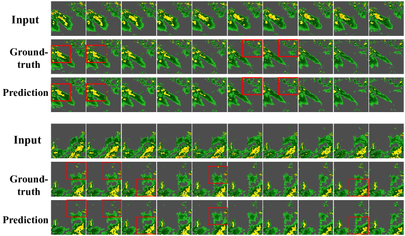
Figure 11: Visualizations of our framework on SEVIR, from which we can find that our model can handle local details very well.

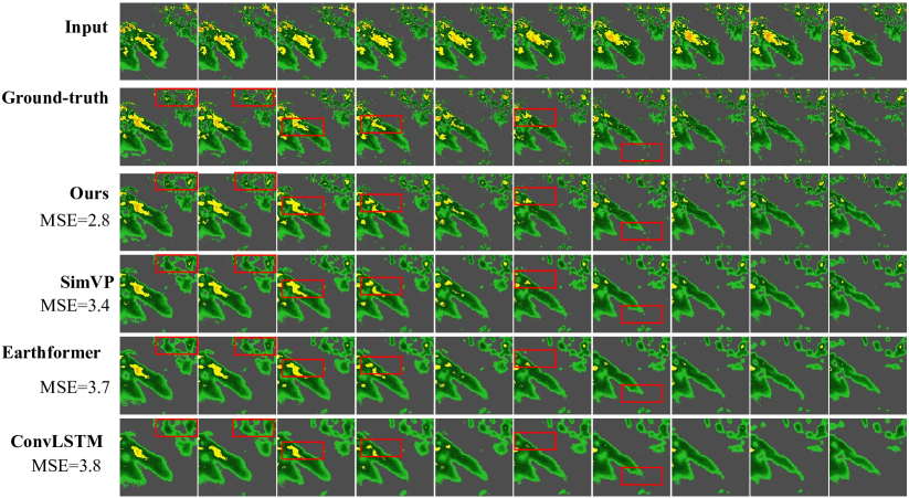
Figure 12: Visualizations of different framework on SEVIR.

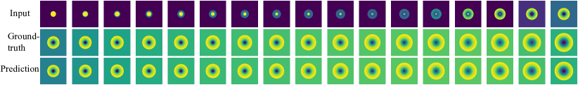
Figure 13: The visualization results are presented every three frames on 2DSWE (50 $\to$ 50) dataset.

Table 5: Performance comparison of various models in long-term prediction of 2D Shallow-Water Equations. The table shows the mean squared error (MSE) and mean absolute error (MAE) of three models: Ours, SimVP, and PDE-STD, with input frames of 20 and output frames of 80. Our model outperformed the other two models, achieving an MSE of 9.8 and an MAE of 57.3.

Model	Input frames	Output frames	MSE	MAE
Ours	$20$	$80$	$9.8$	$57.3$
SimVP	$20$	$80$	$10.7$	$66.6$
PDE-STD	$20$	$80$	$12.3$	$94.8$
Vid-ODE	$20$	$80$	$13.4$	$91.2$
PhyDnet	$20$	$80$	$13.6$	$94.5$

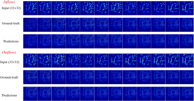
Figure 14: TVisualization of the super-resolution experiment conducted on TaxiBJ+: We downsample the input images to $32\times 32$ pixels and then proceed with predictions at $128\times 128$ pixels. The experimental results clearly demonstrate that our predicted outcomes closely align with the actual outputs, showcasing the scalability of our model in predicting across different pixel sizes.

References

- Anonymous (2023) Anonymous. 2023. NuwaDynamics: Discovering and Updating in Causal Spatio-Temporal Modeling. In Submitted to The Twelfth International Conference on Learning Representations. Under review.
- Ayzel, Scheffer, and Heistermann (2020) Ayzel, G.; Scheffer, T.; and Heistermann, M. 2020. RainNet v1. 0: a convolutional neural network for radar-based precipitation nowcasting. Geoscientific Model Development, 13(6): 2631–2644.
- Bai et al. (2022) Bai, C.; Sun, F.; Zhang, J.; Song, Y.; and Chen, S. 2022. Rainformer: Features extraction balanced network for radar-based precipitation nowcasting. IEEE Geoscience and Remote Sensing Letters, 19: 1–5.
- Benacerraf (1973) Benacerraf, P. 1973. Mathematical truth. The Journal of Philosophy, 70(19): 661–679.
- Chang et al. (2021) Chang, Z.; Zhang, X.; Wang, S.; Ma, S.; Ye, Y.; Xinguang, X.; and Gao, W. 2021. Mau: A motion-aware unit for video prediction and beyond. Advances in Neural Information Processing Systems, 34: 26950–26962.
- Chen et al. (2022a) Chen, B.; Huang, K.; Raghupathi, S.; Chandratreya, I.; Du, Q.; and Lipson, H. 2022a. Automated discovery of fundamental variables hidden in experimental data. Nature Computational Science, 2(7): 433–442.
- Chen et al. (2022b) Chen, X.; Feng, K.; Liu, N.; Ni, B.; Lu, Y.; Tong, Z.; and Liu, Z. 2022b. RainNet: A Large-Scale Imagery Dataset and Benchmark for Spatial Precipitation Downscaling. Advances in Neural Information Processing Systems, 35: 9797–9812.
- Chmiela et al. (2017) Chmiela, S.; Tkatchenko, A.; Sauceda, H. E.; Poltavsky, I.; Schütt, K. T.; and Müller, K.-R. 2017. Machine learning of accurate energy-conserving molecular force fields. Science advances, 3(5): e1603015.
- Donà et al. (2020) Donà, J.; Franceschi, J.-Y.; Lamprier, S.; and Gallinari, P. 2020. Pde-driven spatiotemporal disentanglement. arXiv preprint arXiv:2008.01352.
- Dosovitskiy et al. (2020) Dosovitskiy, A.; Beyer, L.; Kolesnikov, A.; Weissenborn, D.; Zhai, X.; Unterthiner, T.; Dehghani, M.; Minderer, M.; Heigold, G.; Gelly, S.; et al. 2020. An image is worth 16x16 words: Transformers for image recognition at scale. arXiv preprint arXiv:2010.11929.
- Egan and Mahoney (1972) Egan, B. A.; and Mahoney, J. R. 1972. Numerical modeling of advection and diffusion of urban area source pollutants. Journal of Applied Meteorology and Climatology, 11(2): 312–322.
- Gao et al. (2022a) Gao, Z.; Shi, X.; Wang, H.; Zhu, Y.; Wang, Y. B.; Li, M.; and Yeung, D.-Y. 2022a. Earthformer: Exploring space-time transformers for earth system forecasting. Advances in Neural Information Processing Systems, 35: 25390–25403.
- Gao et al. (2022b) Gao, Z.; Tan, C.; Wu, L.; and Li, S. Z. 2022b. Simvp: Simpler yet better video prediction. In Proceedings of the IEEE/CVF Conference on Computer Vision and Pattern Recognition, 3170–3180.
- Greydanus, Dzamba, and Yosinski (2019) Greydanus, S.; Dzamba, M.; and Yosinski, J. 2019. Hamiltonian neural networks. Advances in neural information processing systems, 32.
- Guen and Thome (2020) Guen, V. L.; and Thome, N. 2020. Disentangling physical dynamics from unknown factors for unsupervised video prediction. In Proceedings of the IEEE/CVF Conference on Computer Vision and Pattern Recognition, 11474–11484.
- Guibas et al. (2021a) Guibas, J.; Mardani, M.; Li, Z.; Tao, A.; Anandkumar, A.; and Catanzaro, B. 2021a. Adaptive fourier neural operators: Efficient token mixers for transformers. arXiv preprint arXiv:2111.13587.
- Guibas et al. (2021b) Guibas, J.; Mardani, M.; Li, Z.; Tao, A.; Anandkumar, A.; and Catanzaro, B. 2021b. Adaptive fourier neural operators: Efficient token mixers for transformers. arXiv preprint arXiv:2111.13587.
- Hale and Koçak (2012) Hale, J. K.; and Koçak, H. 2012. Dynamics and bifurcations, volume 3. Springer Science & Business Media.
- Harish and Kumar (2016) Harish, V.; and Kumar, A. 2016. A review on modeling and simulation of building energy systems. Renewable and sustainable energy reviews, 56: 1272–1292.
- Huang et al. (2023) Huang, H.; Xie, S.; Lin, L.; Tong, R.; Chen, Y.-W.; Li, Y.; Wang, H.; Huang, Y.; and Zheng, Y. 2023. SemiCVT: Semi-Supervised Convolutional Vision Transformer for Semantic Segmentation. In Proceedings of the IEEE/CVF Conference on Computer Vision and Pattern Recognition, 11340–11349.
- Humar (2012) Humar, J. 2012. Dynamics of structures. CRC press.
- Isomura and Toyoizumi (2021) Isomura, T.; and Toyoizumi, T. 2021. Dimensionality reduction to maximize prediction generalization capability. Nature Machine Intelligence, 3(5): 434–446.
- Ji et al. (2022) Ji, J.; Wang, J.; Jiang, Z.; Jiang, J.; and Zhang, H. 2022. STDEN: Towards physics-guided neural networks for traffic flow prediction. In Proceedings of the AAAI Conference on Artificial Intelligence, volume 36, 4048–4056.
- Jia et al. (2021) Jia, X.; Willard, J.; Karpatne, A.; Read, J. S.; Zwart, J. A.; Steinbach, M.; and Kumar, V. 2021. Physics-guided machine learning for scientific discovery: An application in simulating lake temperature profiles. ACM/IMS Transactions on Data Science, 2(3): 1–26.
- Kumar et al. (2019) Kumar, M.; Babaeizadeh, M.; Erhan, D.; Finn, C.; Levine, S.; Dinh, L.; and Kingma, D. 2019. Videoflow: A flow-based generative model for video. arXiv preprint arXiv:1903.01434, 2(5): 3.
- Liang et al. (2019) Liang, Y.; Ouyang, K.; Jing, L.; Ruan, S.; Liu, Y.; Zhang, J.; Rosenblum, D. S.; and Zheng, Y. 2019. Urbanfm: Inferring fine-grained urban flows. In Proceedings of the 25th ACM SIGKDD international conference on knowledge discovery & data mining, 3132–3142.
- Liu et al. (2021) Liu, Z.; Lin, Y.; Cao, Y.; Hu, H.; Wei, Y.; Zhang, Z.; Lin, S.; and Guo, B. 2021. Swin transformer: Hierarchical vision transformer using shifted windows. In Proceedings of the IEEE/CVF international conference on computer vision, 10012–10022.
- Liu et al. (2017) Liu, Z.; Yeh, R. A.; Tang, X.; Liu, Y.; and Agarwala, A. 2017. Video frame synthesis using deep voxel flow. 4463–4471.
- Lu et al. (2021) Lu, L.; Jin, P.; Pang, G.; Zhang, Z.; and Karniadakis, G. E. 2021. Learning nonlinear operators via DeepONet based on the universal approximation theorem of operators. Nature machine intelligence, 3(3): 218–229.
- Mathieu, Couprie, and LeCun (2015) Mathieu, M.; Couprie, C.; and LeCun, Y. 2015. Deep multi-scale video prediction beyond mean square error. arXiv preprint arXiv:1511.05440.
- Newell (1980) Newell, A. 1980. Physical symbol systems. Cognitive science, 4(2): 135–183.
- Oh et al. (2015) Oh, J.; Guo, X.; Lee, H.; Lewis, R. L.; and Singh, S. 2015. Action-conditional video prediction using deep networks in atari games. Advances in neural information processing systems, 28.
- Pan et al. (2019a) Pan, J.; Wang, C.; Jia, X.; Shao, J.; Sheng, L.; Yan, J.; and Wang, X. 2019a. Video generation from single semantic label map. 3733–3742.
- Pan et al. (2019b) Pan, Z.; Liang, Y.; Wang, W.; Yu, Y.; Zheng, Y.; and Zhang, J. 2019b. Urban traffic prediction from spatio-temporal data using deep meta learning. In Proceedings of the 25th ACM SIGKDD international conference on knowledge discovery & data mining, 1720–1730.
- Park et al. (2021) Park, S.; Kim, K.; Lee, J.; Choo, J.; Lee, J.; Kim, S.; and Choi, E. 2021. Vid-ode: Continuous-time video generation with neural ordinary differential equation. In Proceedings of the AAAI Conference on Artificial Intelligence, volume 35, 2412–2422.
- Pathak et al. (2022) Pathak, J.; Subramanian, S.; Harrington, P.; Raja, S.; Chattopadhyay, A.; Mardani, M.; Kurth, T.; Hall, D.; Li, Z.; Azizzadenesheli, K.; et al. 2022. Fourcastnet: A global data-driven high-resolution weather model using adaptive fourier neural operators. arXiv preprint arXiv:2202.11214.
- Pierson (1993) Pierson, S. 1993. Corpore cadente…: Historians Discuss Newton’s Second Law. Perspectives on Science, 1(4): 627–658.
- Schuldt, Laptev, and Caputo (2004) Schuldt, C.; Laptev, I.; and Caputo, B. 2004. Recognizing human actions: a local SVM approach. In Proceedings of the 17th International Conference on Pattern Recognition, 2004. ICPR 2004., volume 3, 32–36. IEEE.
- Sharan et al. (1996) Sharan, M.; Yadav, A. K.; Singh, M.; Agarwal, P.; and Nigam, S. 1996. A mathematical model for the dispersion of air pollutants in low wind conditions. Atmospheric Environment, 30(8): 1209–1220.
- Shi et al. (2015) Shi, X.; Chen, Z.; Wang, H.; Yeung, D.-Y.; kin Wong, W.; and chun Woo, W. 2015. Convolutional LSTM Network: A Machine Learning Approach for Precipitation Nowcasting. arXiv:1506.04214.
- Srivastava, Mansimov, and Salakhudinov (2015) Srivastava, N.; Mansimov, E.; and Salakhudinov, R. 2015. Unsupervised learning of video representations using lstms. In International conference on machine learning, 843–852. PMLR.
- Takamoto et al. (2022) Takamoto, M.; Praditia, T.; Leiteritz, R.; MacKinlay, D.; Alesiani, F.; Pflüger, D.; and Niepert, M. 2022. PDEBench: An extensive benchmark for scientific machine learning. Advances in Neural Information Processing Systems, 35: 1596–1611.
- Tan et al. (2022) Tan, C.; Gao, Z.; Li, S.; and Li, S. Z. 2022. Simvp: Towards simple yet powerful spatiotemporal predictive learning. arXiv preprint arXiv:2211.12509.
- Tulyakov et al. (2018) Tulyakov, S.; Liu, M.-Y.; Yang, X.; and Kautz, J. 2018. Mocogan: Decomposing motion and content for video generation. In Proceedings of the IEEE conference on computer vision and pattern recognition, 1526–1535.
- Veillette, Samsi, and Mattioli (2020) Veillette, M.; Samsi, S.; and Mattioli, C. 2020. Sevir: A storm event imagery dataset for deep learning applications in radar and satellite meteorology. Advances in Neural Information Processing Systems, 33: 22009–22019.
- Walker, Razavi, and Oord (2021) Walker, J.; Razavi, A.; and Oord, A. v. d. 2021. Predicting video with vqvae. arXiv preprint arXiv:2103.01950.
- Wang et al. (2023a) Wang, K.; Li, G.; Wang, S.; Zhang, G.; Wang, K.; You, Y.; Peng, X.; Liang, Y.; and Wang, Y. 2023a. The snowflake hypothesis: Training deep GNN with one node one receptive field. arXiv preprint arXiv:2308.10051.
- Wang et al. (2023b) Wang, K.; Liang, Y.; Li, X.; Li, G.; Ghanem, B.; Zimmermann, R.; Yi, H.; Zhang, Y.; Wang, Y.; et al. 2023b. Brave the Wind and the Waves: Discovering Robust and Generalizable Graph Lottery Tickets. IEEE Transactions on Pattern Analysis and Machine Intelligence.
- Wang et al. (2022a) Wang, K.; Liang, Y.; Wang, P.; Wang, X.; Gu, P.; Fang, J.; and Wang, Y. 2022a. Searching Lottery Tickets in Graph Neural Networks: A Dual Perspective. In The Eleventh International Conference on Learning Representations.
- Wang et al. (2022b) Wang, K.; Zhou, Z.; Wang, X.; Wang, P.; Fang, Q.; and Wang, Y. 2022b. A2DJP: A two graph-based component fused learning framework for urban anomaly distribution and duration joint-prediction. IEEE Transactions on Knowledge and Data Engineering.
- Wang, Cao, and Philip (2020) Wang, S.; Cao, J.; and Philip, S. Y. 2020. Deep learning for spatio-temporal data mining: A survey. IEEE transactions on knowledge and data engineering, 34(8): 3681–3700.
- Wang et al. (2019) Wang, Y.; Jiang, L.; Yang, M.-H.; Li, L.-J.; Long, M.; and Fei-Fei, L. 2019. Eidetic 3D LSTM: A Model for Video Prediction and Beyond. In International Conference on Learning Representations.
- Wang et al. (2022c) Wang, Y.; Wu, H.; Zhang, J.; Gao, Z.; Wang, J.; Philip, S. Y.; and Long, M. 2022c. Predrnn: A recurrent neural network for spatiotemporal predictive learning. IEEE Transactions on Pattern Analysis and Machine Intelligence, 45(2): 2208–2225.
- Weissenborn, Täckström, and Uszkoreit (2019) Weissenborn, D.; Täckström, O.; and Uszkoreit, J. 2019. Scaling autoregressive video models. arXiv preprint arXiv:1906.02634.
- Wiggins, Wiggins, and Golubitsky (2003) Wiggins, S.; Wiggins, S.; and Golubitsky, M. 2003. Introduction to applied nonlinear dynamical systems and chaos, volume 2. Springer.
- Wu et al. (2023) Wu, H.; Xion, W.; Xu, F.; Luo, X.; Chen, C.; Hua, X.-S.; and Wang, H. 2023. PastNet: Introducing Physical Inductive Biases for Spatio-temporal Video Prediction. arXiv preprint arXiv:2305.11421.
- Yang et al. (2022) Yang, T.-Y.; Rosca, J.; Narasimhan, K.; and Ramadge, P. J. 2022. Learning Physics Constrained Dynamics Using Autoencoders. Advances in Neural Information Processing Systems, 35: 17157–17172.