The complex-step Newton method and its convergence

Abstract.

Considered herein is a Jacobian-free Newton method for the numerical solution of nonlinear equations where the Jacobian is approximated using the complex-step derivative approximation. We demonstrate that this method converges for complex-step values sufficiently small and not necessarily tiny. Notably, in the case of scalar equations the convergence rate becomes quadratic as the complex-step tends to zero. On the other hand, in the case of systems of equations the rate is quadratic for any appropriately small value of the complex-step and not just in the limit to zero. This assertion is substantiated through numerical experiments. Furthermore, we demonstrate the method’s seamless applicability in solving nonlinear systems that arise in the context of differential equations, employing it as a Jacobian-free Newton-Krylov method.

1. Introduction

The subject of this paper is the study of a Jacobian-free Newton method known as complex-step Newton method for approximating roots of smooth functions. Jacobian-free Newton methods are significant for two primary reasons: (i) they operate effectively even when the Jacobian matrix (or the derivative in scalar cases) is unavailable, and (ii) they can be integrated with Krylov solvers to enhance their efficiency in solving systems of equations [9]. One example of such a method is the complex-step Newton method as it is demonstrated by [4]. In what follows $h$ is assumed to be a fixed positive constant. Assume that we search for the solution $x^{\ast}$ of an equation $f(x)=0$ where $f:I\subset\mathbb{R}\to\mathbb{R}$ is appropriately smooth function and $I$ an interval that includes in its interior the root $x^{\ast}$. Then, the first derivative, $f^{\prime}(x)$, can be approximated as $f^{\prime}(x)\approx\mathrm{Im}f(x+\mathrm{i}h)/h$ [10, 17]. The parameter $h$ is referred to as the complex step, and the method itself is named after this parameter. Replacing the classical derivative by its complex-step approximation, the complex-step Newton iteration can be expressed in the following form:

$$x_{k+1}=x_{k}-h\frac{f(x_{k})}{\mathrm{Im}f(x_{k}+\mathrm{i}h)}\quad\text{for $k=0,1,\dots$}\ ,$$

where $\mathrm{i}=\sqrt{-1}$ denotes the imaginary unit.

Similarly, the complex-step Newton iteration can be applied to systems of equations of the form $\mathbf{F}(\mathbf{x})=\mathbf{0}$, where $\mathbf{x}\in\mathbb{R}^{n}$ and $\mathbf{F}:D\subset\mathbb{R}^{n}\to\mathbb{R}^{n}$ for $n\geq 2$. Specifically, the Jacobian matrix can be approximated by the matrix with entries

$$[\mathbf{J}_{h}(\mathbf{x})]_{ij}=\frac{1}{h}\mathrm{Im}F_{i}(\mathbf{x}+\mathrm{i}h\mathbf{e}_{j})\quad\text{for any $h>0$}\ ,$$

where $\mathbf{e}_{j}$ denotes the usual basis of $\mathbb{R}^{n}$. The complex-step Newton method for the system $\mathbf{F}(\mathbf{x})=\mathbf{0}$ is the iteration

(1) $$\mathbf{x}^{(k+1)}=\mathbf{x}^{(k)}-\mathbf{J}_{h}^{-1}(\mathbf{x}^{(k)})\mathbf{F}(\mathbf{x}^{(k)})\quad\text{for k=0,1,2,\ldots\ .}$$

What values of $h$ lead to convergence and at what rate is a critical question for the complex-step Newton method. The answer to this questions can lead to the use of this method in lower precision arithmetic, [7], and contributes to our confidence in its use. In this article we focus on the rigorous study of the convergence of the complex-step Newton method. In Section 2, following a rigorous derivation of the complex-step Newton iteration, we establish its convergence for sufficiently small values of $h$. Specifically, we show that for the scalar case the convergence becomes quadratic as $h$ tends to 0. However, when dealing with systems of equations, we demonstrate that the complex-step Newton method exhibits a quadratic rate of convergence for not necessarily tiny values of $h$. We empirically validate these results and conclude this paper with a study of the effects of the parameter $h$ in various applications. In Section 3 we demonstrate the use of the complex-step Newton method for the solution of nonlinear systems obtained during the numerical integration of stiff ordinary differential equations by a symplectic Runge-Kutta method, namely, the fourth-order Gauss-Legendre Runge-Kutta method of order four [16]. Moreover, in the same section we consider the discrete nonlinear Schrödinger (DNLS) equation [8]. First we obtain a steady-state solution of this equation by solving the corresponding nonlinear system of equations using the complex-step Newton method. Then we employ the implicit fourth-order Gauss-Legendre Runge-Kutta method for the time discretization of the ODE system of the corresponding DNLS equation. Due to its symplectic nature, the particular time-integration method demonstrates excellent conservation properties by preserving the norm (quadratic integral) while almost conserving the Hamiltonian [2]. This suggests that using the complex-step Newton method in conjunction with a Krylov method, without strict constraints on the parameter $h$, creates an optimal combination for these problems due to its straightforward implementation.

2. Convergence

2.1. Scalar equations

First we review the derivation of the complex-step Newton iteration. Consider the equation $f(x)=0$ where $f:I\to\mathbb{R}$ is a real analytic function in a closed interval $I\subset\mathbb{R}$ appropriately chosen such that $f^{\prime}(x)\not=0$ for all $x\in I$. We assume that this equation has a unique solution $x^{\ast}\in I$. Given $x_{0}\in I$, we define the classical Newton iteration as

(2) $$x_{k+1}=x_{k}-\frac{f(x_{k})}{f^{\prime}(x_{k})}\quad\text{for $k=0,1,\dots$}\ .$$

In order to estimate alternatives of the first derivative using complex number arithmetic ([10, 17]) we consider the Taylor expansion of the function $g(h)=\mathrm{Im}f(x+\mathrm{i}h)$ for $x\in I$ and $h\in\mathbb{R}$ around $h=0$

(3) $$g(h)=g(0)+g^{\prime}(0)h+\frac{g^{\prime\prime}(0)}{2}h^{2}+\frac{g^{\prime\prime\prime}(c_{h})}{6}h^{3}\ ,$$

where $0<c_{h}<h$. Obviously it is $g(0)=0$. Writing $f(x+\mathrm{i}h)=r(x,h)+\mathrm{i}s(x,h)=r(x,h)+\mathrm{i}g(h)$ we have that $g^{\prime}(h)=s_{h}(x,h)$, where the subscript $h$ here denotes partial differentiation with respect of $h$. On the other hand, $\frac{d}{dh}f(x+\mathrm{i}h)=\mathrm{i}f^{\prime}(x+\mathrm{i}h)=r_{h}(x,h)+\mathrm{i}s_{h}(x,h)=r_{h}(x,h)+\mathrm{i}g^{\prime}(h)$. Thus, for $h=0$ we have $\mathrm{i}f^{\prime}(x)=r_{h}(x,0)+\mathrm{i}g^{\prime}(0)$. Taking the imaginary part of both sides we obtain $g^{\prime}(0)=f^{\prime}(x)$. Note that the derivative in the last formula coincides with the real derivative $f^{\prime}(x)$ due to the path-independence of the complex derivatives. Similarly, since $\frac{d^{2}}{dh^{2}}f(x+\mathrm{i}h)=-f^{\prime\prime}(x+\mathrm{i}h)=r_{hh}(x,h)+\mathrm{i}s_{hh}(x,h)$ we have $g^{\prime\prime}(0)=s_{hh}(x,0)=0$. Finally, $\frac{d^{3}}{dh^{3}}f(x+\mathrm{i}h)=-\mathrm{i}f^{\prime\prime\prime}(x+\mathrm{i}h)=r_{hhh}(x,h)+\mathrm{i}g^{\prime\prime\prime}(h)$ and thus $g^{\prime\prime\prime}(c_{h})=-\mathrm{Im}[\mathrm{i}f^{\prime\prime\prime}(x+\mathrm{i}c_{h})]$. Combining the previous formulas in (3) we obtain to the relation

(4) $$f^{\prime}(x)=\frac{1}{h}\mathrm{Im}f(x+\mathrm{i}h)+R^{x}(c_{h})h^{2}\ ,$$

with $R^{x}(c_{h})=\tfrac{1}{6}\mathrm{Im}[\mathrm{i}f^{\prime\prime\prime}(x+\mathrm{i}c_{h})]$. The approximation of the first derivative $f^{\prime}(x)$ by $\mathrm{Im}f(x+\mathrm{i}h)/h$ is called the complex-step approximation and it does not suffer from cancellation errors like the standard finite difference formulas for values of $h$ even of the order $10^{-20}$ and less, [10, 17]. For this reason we can approximate the first derivative up to the machine precision. Based on this approximation, the complex-step Newton iteration is defined as

(5) $$x_{k+1}=x_{k}-h\frac{f(x_{k})}{\mathrm{Im}f(x_{k}+\mathrm{i}h)}\quad\text{for $k=0,1,\dots$}\ .$$

The assumption that $f$ is real analytic in an interval containing the root $x^{\ast}$ can be relaxed; however, it ensures the extension of $f$ into a complex analytic function within a region surrounding the root $x^{\ast}$. For example if $f(x)=\sum_{n}a_{n}(x-x^{\ast})^{n}$ for $x\in D$, where $D$ is closed interval that includes $x^{\ast}$ in its interior, then there is an $\varepsilon>0$ such that the analytic complex extension of $f$ can be defined as $f(z)=\sum_{n}a_{n}(z-x^{\ast})^{n}$ in $D\times[-\mathrm{i}\varepsilon,\mathrm{i}\varepsilon]$. This extension guarantees that the derivatives of $f$ remain uniformly bounded within a closed region of the complex domain, as per Cauchy’s integral formula [1, Section 2.6.2]. The assumption of uniformly bounded first and third derivatives is necessary, as elucidated in the subsequent proofs. In general, we will denote by $C$ any generic positive constant independent of $h$.

Lemma 2.1.

If the function $f$ is real analytic in a closed interval $I$ and $x^{\ast}$ in the interior of $I$ with $f(x^{\ast})=0$ and $f^{\prime}(x^{\ast})\not=0$, then there are $\bar{h}>0$ and $m,M>0$ independent of $h$ such that $m\leq\frac{1}{h}|\mathrm{Im}f(x+ih)|\leq M$ for all $0<h<\bar{h}$.

Proof.

Since $f^{\prime}(x^{\ast})\not=0$ there is a neighborhood $J\subset I$ with $x^{\ast}\in J$ and $m^{\prime},M^{\prime}>0$ such that $m^{\prime}<|f^{\prime}(x)|<M^{\prime}$ for all $x\in I^{\prime}$. Furthermore, due to the analyticity of $f$, there is a closed neighborhood $\mathbb{D}\subset\mathbb{C}$ around $x^{\ast}$ and a $K>0$ such that $|f^{\prime\prime\prime}(z)|<K$ for all $z\in\mathbb{D}$.

From (4) we have

$$\left|\tfrac{1}{h}\mathrm{Im}f(x+\mathrm{i}h)\right|\leq|f^{\prime}(x)|+|R^{x}(c_{h})|h^{2}<M^{\prime}+|R^{x}(c_{h})|h^{2}\ ,$$

and thus there is an $h_{1}>0$ such that $|\mathrm{Im}f(x+\mathrm{i}h)|/h\leq 2M^{\prime}$ for all $0<h<h_{1}$. Similarly,

$$\left|\tfrac{1}{h}\mathrm{Im}f(x+\mathrm{i}h)\right|\geq|f^{\prime}(x)|-|R^{x}(c_{h})|h^{2}>m^{\prime}-|R^{x}(c_{h})|h^{2}\ ,$$

which yields that there is an $h_{2}>0$ such that $|\mathrm{Im}f(x+\mathrm{i}h)|/h\geq m^{\prime}/2$, for $0<h<h_{2}$. We take $\bar{h}=\min(h_{1},h_{2})$, $m=m^{\prime}/2$ and $M=2M^{\prime}$. ∎

Now we can prove that the complex-step Newton iteration converges and for small values of $h$ the convergence is linear and in practical terms $h\to 0$ becomes quadratic.

Theorem 2.1.

Given a real analytic function $f$ in a closed interval $I$ and $x^{\ast}$ in the interior of $I$ with $f(x^{\ast})=0$ and $f^{\prime}(x^{\ast})\not=0$, then there is $h_{0}>0$ and an interval $D\subset I$ such that the complex-step Newton iteration $x_{k}$ of (5) converges to the exact solution $x^{\ast}$ of the equation $f(x)=0$ for all $x_{0}\in D$ and for all $0<h<h_{0}$. Furthermore,

(6) $$\lim_{k\to\infty}\left[\lim_{h\to 0}\frac{x_{k+1}-x^{\ast}}{(x_{k}-x^{\ast})^{2}}\right]=\frac{f^{\prime\prime}(x^{\ast})}{2f^{\prime}(x^{\ast})}\ .$$

Proof.

First we establish the convergence of the method by recalling that the conditions of Lemma 2.1 imply the existence of constants $m,M>0$, such that $m<|f^{\prime}(x)|<M$ for all $x\in J$ where $J\subset I$. Additionally, there exists a closed neighborhood $\mathbb{D}\subset\mathbb{C}$ of $x^{\ast}$ and a constant $K>0$ such that $|f^{\prime\prime\prime}(z)|<K$ for all $z\in\mathbb{D}$. Having established in Lemma 2.1 that the complex-step approximation of the derivative is bounded by a bound that is independent of $h$ for $0<h<\bar{h}$, we rewrite (4) as

(7) $$h\frac{f^{\prime}(x)}{\mathrm{Im}f(x+\mathrm{i}h)}=1+\tilde{R}(c_{h})h^{2}\ ,$$

where $\tilde{R}(c_{h})=\frac{R^{x}(c_{h})}{\tfrac{1}{h}\mathrm{Im}f(x+\mathrm{i}h)}$. Using the lower bound of the complex-step approximation, we have $|\tilde{R}(c_{h})|\leq|R^{x}(c_{h})|/m$. Thus we have that $|\tilde{R}(c_{h})|\leq K/6m$ where the bound is independent of $h$.

The complex-step Newton iteration (5) is written as a fixed point equation $x_{k+1}=G_{h}(x_{k})$, for $k=0,1,\dots$ where

$$G_{h}(x)=x-h\frac{f(x)}{\mathrm{Im}f(x+\mathrm{i}h)}\ .$$

Taking into account that $f$ is analytic, (7) and that $f(x^{\ast})=0$, we have that

(8) $$G^{\prime}_{h}(x^{\ast})=1-h\frac{f^{\prime}(x^{\ast})}{\mathrm{Im}f(x^{\ast}+\mathrm{i}h)}=-\tilde{R}(c_{h})h^{2}\ .$$

From Lemma 2.1 and the previous comments we deduce that there is an $\bar{h}>0$ such that for $h\in(0,\bar{h})$ the derivative $|G^{\prime}_{h}(x^{\ast})|\leq Ch^{2}<1$ and thus $G_{h}$ is a contraction, and we conclude by the fixed point theorem (cf. [13]) that there is a neighborhood $D$ of $x^{\ast}$ such that for any $x_{0}\in D$ the iteration $x_{k+1}=G_{h}(x_{k})$ converges to $x^{\ast}$ as $k\to\infty$. In the sequel we denote the error of the approximation by $e_{k}=x_{k}-x^{\ast}$, and thus we have that $\lim_{k\to\infty}e_{k}=0$.

Since $f$ is analytic, we have the following Taylor expansions for the function $f$,

(9) $$f(x_{k})=f(x^{\ast})+(x_{k}-x^{\ast})f^{\prime}(x^{\ast})+\frac{(x_{k}-x^{\ast})^{2}}{2}f^{\prime\prime}(c_{k})=e_{k}f^{\prime}(x^{\ast})+\frac{e_{k}^{2}}{2}f^{\prime\prime}(c_{k})\ ,$$

and its derivative

(10) $$\frac{1}{h}\mathrm{Im}f(x_{k}+\mathrm{i}h)=f^{\prime}(x_{k})-R^{x}(c_{h})h^{2}=f^{\prime}(x^{\ast})+e_{k}f^{\prime\prime}(d_{k})-R^{x}(c_{h})h^{2}\ ,$$

where $c_{k}$ and $d_{k}$ are constants between $x^{\ast}$ and $x_{k}$, while $0<c_{h}<h$ as before. Substituting these expansions into (5) we obtain

(11) $$x_{k+1}=x_{k}-\frac{e_{k}f^{\prime}(x^{\ast})+\frac{e_{k}^{2}}{2}f^{\prime\prime}(c_{k})}{f^{\prime}(x^{\ast})+e_{k}f^{\prime\prime}(d_{k})-R^{x}(c_{h})h^{2}}\ .$$

Subtracting $x^{\ast}$ from both sides and denoting $e_{k}=x^{k}-x^{\ast}$ the error at the $k$-th iteration, the last equation yields

$$e_{k+1} =e_{k}-\frac{e_{k}f^{\prime}(x^{\ast})+\frac{e_{k}^{2}}{2}f^{\prime\prime}(c_{k})}{f^{\prime}(x^{\ast})+e_{k}f^{\prime\prime}(d_{k})-R^{x}(c_{h})h^{2}}$$

(12) $$=e_{k}^{2}\frac{f^{\prime\prime}(d_{k})-\tfrac{1}{2}f^{\prime\prime}(c_{k})}{f^{\prime}(x^{\ast})+e_{k}f^{\prime\prime}(d_{k})-R^{x}(c_{h})h^{2}}-e_{k}\frac{R^{x}(c_{h})h^{2}}{f^{\prime}(x^{\ast})+e_{k}f^{\prime\prime}(d_{k})-R^{x}(c_{h})h^{2}}\ .$$

From this we extract two pieces of information. First, dividing by $e_{k}$ and taking the limit $k\to\infty$ we have that

$$\lim_{k\to\infty}\frac{e_{k+1}}{e_{k}}=-\frac{R^{x}(c_{h})h^{2}}{f^{\prime}(x^{\ast})-R^{x}(c_{h})h^{2}}\ .$$

Let $B=\sup_{z\in\mathbb{D}}|f^{\prime\prime\prime}(z)|>0$ where $\mathbb{D}$ is a neighborhood of $x^{\ast}$, we define $h_{1}=\sqrt{3|f^{\prime}(x^{\ast})|/B}$. Then for $0<h<h_{0}=\min\{\bar{h},h_{1}\}$ we have that

$$\frac{|R^{x}(c_{h})h^{2}|}{|f^{\prime}(x^{\ast})-R^{x}(c_{h})h^{2}|}\leq\frac{1}{\frac{|f^{\prime}(x^{\ast})|}{|R^{x}(c_{h})h^{2}|}-1}<1\ .$$

Therefore, the complex-step Newton method converges for all $h<h_{0}$.

Moreover, we see that the error behaves better as $h\to 0$. From equation (8) we have that $\lim_{h\to 0}G^{\prime}_{h}(x^{\ast})=0$, and thus

$$\lim_{h\to 0}\frac{x_{k+1}-x^{\ast}}{x_{k}-x^{\ast}}=\lim_{h\to 0}\frac{G_{h}(x_{k})-G_{h}(x^{\ast})}{x_{k}-x^{\ast}}=\lim_{h\to 0}\left[\frac{G_{h}(x_{k})-G_{h}(x^{\ast})}{x_{k}-x^{\ast}}-G^{\prime}_{h}(x^{\ast})\right]\ .$$

Thus,

$$\lim_{k\to\infty}\left[\lim_{h\to 0}\frac{e_{k+1}}{e_{k}}\right]=0\ .$$

Further to that we have from (12) that

$$\frac{e_{k+1}}{e_{k}^{2}}=\frac{f^{\prime\prime}(d_{k})-\tfrac{1}{2}f^{\prime\prime}(c_{k})}{f^{\prime}(x^{\ast})+e_{k}f^{\prime\prime}(d_{k})-R^{x}(c_{h})h^{2}}-\frac{R^{x}(c_{h})h^{2}}{e_{k}[f^{\prime}(x^{\ast})+e_{k}f^{\prime\prime}(d_{k})-R^{x}(c_{h})h^{2}]}\ ,$$

and more precisely, by taking $h\to 0$ we obtain

$$\lim_{h\to 0}\frac{e_{k+1}}{e_{k}^{2}}=\frac{f^{\prime\prime}(d_{k})-\tfrac{1}{2}f^{\prime\prime}(c_{k})}{f^{\prime}(x^{\ast})+e_{k}f^{\prime\prime}(d_{k})}\ ,$$

and thus

$$\lim_{k\to\infty}\left[\lim_{h\to 0}\frac{e_{k+1}}{e_{k}^{2}}\right]=\frac{f^{\prime\prime}(x^{\ast})}{2f^{\prime}(x^{\ast})}\ ,$$

since both $c_{k}\to x^{\ast}$ and $d_{k}\to x^{\ast}$ as $k\to\infty$, which completes the proof. ∎

This result implies that for sufficiently small values of $h\ll 1$, the observed convergence will be quadratic. We experimentally study the convergence and the influence of the complex-step $h$ on the convergence using the simple equation $f(x)=0$ with $f(x)=x(e^{x/2}+1)$, where $x^{\ast}=0$ is an obvious root. Moreover, $f^{\prime}(x^{\ast})\neq 0$, and the above theory is applied to this case in a straightforward manner. In order to study the influence of $h$ we consider the values $h=2/n$ for $n=1,2,\dots,10^{6}$. Figure 1 presents the experimental convergence rate $\log|e_{k+1}/e_{k}|/\log|e_{k}/e_{k-1}|$ where $e_{k}=x_{k}-x^{\ast}$ as a function of $h$. As convergence criterion we used the inequality $|x_{k}-x^{\ast}|\leq 10^{-12}$ and initial guess $x_{0}=2.5$.

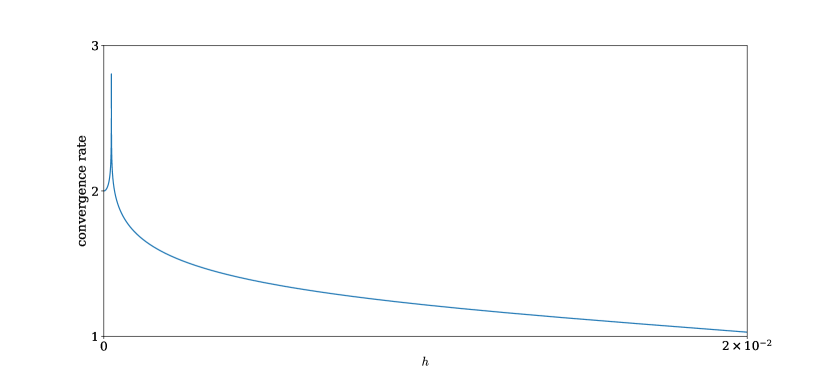
Figure 1. Convergence rate and number of iterations as a function of $h$ for a scalar function $f$

We observe that the method converged clearly with rate $1$ for large values of $h$ while it accelerates after a threshold value. The maximum convergence rate was observed for $h\approx 0.00023635$. As $h$ became much smaller than $1$, the convergence rate was stabilized to $2$ as predicted by the Theorem 2.1, while for values of $h$ of $O(1)$ we observe that the convergence rate is 1. In all cases the error became smaller than the tolerance within 6 iterations. Similar behaviour can also be observed if we choose the tolerance to be $10^{-15}$ with the difference that the errors will become very small after the sixth iteration that can be hardly distinguished from the machine precision. We proceed next with the study of the complex-step Newton method for systems of algebraic equations, where the situation is slightly different.

2.2. Systems of equations

Consider a system of equations of the form $\mathbf{F}(\mathbf{x})=\mathbf{0}$ where $\mathbf{F}:U\subset\mathbb{R}^{n}\to\mathbb{R}^{n}$ is a vector valued function $\mathbf{F}=(F_{1},F_{2},\dots,F_{n})^{T}$ with $n\geq 2$. We assume that $F_{i}$ are real analytic functions on $U$ and $\mathbf{x}=(x_{1},x_{2},\dots,x_{n})^{T}$. In this way, all the derivatives of $F_{i}$ can be extended to complex analytic functions in a closed neighborhood of $\mathbf{x}^{\ast}$ similarly to the one-dimensional case. Moreover, $\mathbf{F}$ is Fréchet-differentiable in a neighborhood of $\mathbf{x}^{\ast}$. Given $\mathbf{x}^{(0)}\in U$, we define the classical Newton iteration as

$$\mathbf{x}^{(k+1)}=\mathbf{x}^{(k)}-\mathbf{DF}^{-1}(\mathbf{x}^{(k)})\mathbf{F}(\mathbf{x}^{(k)})\quad\text{for $k=0,1,\dots$}\ ,$$

where the $\mathbf{DF}$ is the Jacobian matrix with entries the derivatives $[\mathbf{DF}]_{i,j}=\partial_{j}F_{i}$ where $\partial_{j}=\frac{\partial}{\partial x_{j}}$. For convenience in the implementation we usually express the general Newton iteration by the following linear system of equations

$$\mathbf{DF}(\mathbf{x}^{(k)})\mathbf{u}^{(k)}=\mathbf{F}(\mathbf{x}^{(k)}),\qquad\mathbf{x}^{(k+1)}=\mathbf{x}^{(k)}-\mathbf{u}^{(k)},\quad\text{for $k=0,1,\dots$}\ .$$

Working similarly as in Section 2.1 we assume that the function $\mathbf{F}$ can be extended in the neighborhood of $\mathbf{x}^{\ast}$ in the complex space and that for $\mathbf{z}=\mathbf{x}+\mathrm{i}\mathbf{y}$ we can write $\mathbf{F}(\mathbf{z})=\mathbf{r}(\mathbf{x},\mathbf{y})+\mathrm{i}\mathbf{s}(\mathbf{x},\mathbf{y})$, where $\mathbf{s}(\mathbf{x},\mathbf{y})=\mathrm{Im}\mathbf{F}(\mathbf{z})$. We set $\mathbf{g}(h)=\mathrm{Im}\mathbf{F}(\mathbf{x}+\mathrm{i}h\mathbf{v})=\mathbf{s}(\mathbf{x},h\mathbf{v})$ where $\mathbf{v}\in\mathbb{R}^{n}$. This implies that $\mathbf{g}^{\prime}(h)=\nabla_{\mathbf{y}}\mathbf{s}(\mathbf{x},h\mathbf{v})\mathbf{v}$, where $\nabla_{\mathbf{y}}\mathbf{s}$ denotes the Jacobian matrix of $\mathbf{s}(\mathbf{x},\mathbf{y})$ with respect to vector $\mathbf{y}$. On the other hand, if $\nabla_{\mathbf{z}}\mathbf{F}(\mathbf{z})$ denotes the complex Jacobian matrix with entries $[\partial F_{i}/\partial z_{j}]_{ij}$, then $\partial_{h}\mathbf{F}(\mathbf{x}+\mathrm{i}h\mathbf{v})=\mathrm{i}\nabla_{\mathbf{z}}\mathbf{F}(\mathbf{x}+\mathrm{i}h\mathbf{v})\mathbf{v}=\nabla_{\mathbf{y}}\mathbf{r}(\mathbf{x},h\mathbf{v})\mathbf{v}+\mathrm{i}\nabla_{\mathbf{y}}\mathbf{s}(\mathbf{x},h\mathbf{v})\mathbf{v}$. Thus, we have that $\mathbf{g}^{\prime}(0)=\nabla_{\mathbf{y}}\mathbf{s}(\mathbf{x},0)\mathbf{v}=\nabla_{\mathbf{z}}\mathbf{F}(\mathbf{x})\mathbf{v}=\mathbf{D}\mathbf{F}(\mathbf{x})\mathbf{v}$, where the last equality holds because of the path-independence of complex derivatives.

Then, the Taylor expansion of $g$ about $h=0$ will be

$$\mathbf{g}(h)=\mathbf{g}(0)+\mathbf{g}^{\prime}(0)h+\frac{\mathbf{g}^{\prime\prime}(0)}{2}h^{2}+\frac{\mathbf{g}^{\prime\prime\prime}(c_{h})}{6}h^{3}\ ,$$

here $0<c_{h}<h$, while $\mathbf{g}(0)=\mathbf{0}$, $\mathbf{g}^{\prime}(0)=\mathbf{DF}(\mathbf{x})\mathbf{v}$, $\mathbf{g}^{\prime\prime}(0)=\mathbf{0}$ and we denote the third derivative vector $-\mathbf{g}^{\prime\prime\prime}(c_{h})/6$ as $\mathbf{R}^{\mathbf{x}}(c_{h})=\mathbf{R}^{\mathbf{x}}(c_{h};\mathbf{v})$ that depends on $\mathbf{v}$ and has $\ell$-entry (cf. [18])

$$[\mathbf{R}^{\mathbf{x}}(c_{h};\mathbf{v})]_{\ell}=-\frac{[\mathbf{g}^{\prime\prime\prime}(c_{h})]_{\ell}}{6}=\frac{1}{6}\sum_{i,j,k=1}^{n}\mathrm{Im}\left[\mathrm{i}\frac{\partial^{3}F_{\ell}(\mathbf{x}+\mathrm{i}c_{h}\mathbf{v})}{\partial v_{i}\partial v_{j}\partial v_{k}}v_{i}v_{j}v_{k}\right]\ .$$

Taking absolute values we obtain the bounds

$$|[\mathbf{R}^{\mathbf{x}}(c_{h};\mathbf{v})]_{\ell}|\leq\frac{1}{6}\sum_{i,j,k=1}^{n}\left|\mathrm{Im}\left[\mathrm{i}\frac{\partial^{3}F_{\ell}(\mathbf{x}+\mathrm{i}c_{h}\mathbf{v})}{\partial v_{i}\partial v_{j}\partial v_{k}}\right]\right|\|\mathbf{v}\|^{3}\ .$$

Further we assume that the third-order derivatives of $\mathbf{F}(\mathbf{z})$ are uniformly bounded by a bound independent of $h$, which can be ensured by the analyticity of $\mathbf{F}$ in a closed region of the complex spaces that includes in its interior the solution $\mathbf{x}^{\ast}$. If for example we assume that there is a constant $K\geq 0$ (independent of $h$) such that $|\partial^{3}F_{\ell}(\mathbf{z})/\partial z_{i}\partial z_{j}\partial z_{k}|\leq K$ uniformly for all $\mathbf{z}$ in a closed neighborhood of $\mathbf{x}^{\ast}$ and for all $i,j,k,\ell=1,2,\dots,n$, then we have that

(13) $$\|\mathbf{R}^{\mathbf{x}}(c_{h};\mathbf{v})\|\leq C\|\mathbf{v}\|^{3}\ ,$$

where $C>0$ is independent of $h$. This leads to the approximation

(14) $$\mathbf{DF}(\mathbf{x})\mathbf{v}=\frac{1}{h}\mathrm{Im}\mathbf{F}(\mathbf{x}+\mathrm{i}h\mathbf{v})+\mathbf{R}^{\mathbf{x}}(c_{h};\mathbf{v})h^{2}\ .$$

Denote the unit normal basis vectors of $\mathbb{R}^{n}$ by $\mathbf{e}_{j}$, and write $\mathbf{v}=\sum_{j=1}^{n}v_{j}\mathbf{e}_{j}$. Then

$$\mathbf{DF}(\mathbf{x})\mathbf{v}=\sum_{j=1}^{n}v_{j}\mathbf{DF}(\mathbf{x})\mathbf{e}_{j}=\sum_{j=1}^{n}v_{j}\frac{1}{h}\mathrm{Im}\mathbf{F}(\mathbf{x}+\mathrm{i}h\mathbf{e}_{j})+\mathbf{R}^{\mathbf{x}}(c_{h};\mathbf{v})h^{2}\ .$$

It is natural then to consider the approximation

(15) $$\partial_{j}F_{i}(\mathbf{x})\approx\frac{1}{h}[\mathrm{Im}\mathbf{F}(\mathbf{x}+\mathrm{i}h\mathbf{e}_{j})]_{i}\ ,$$

which agrees with the one-dimensional complex-step approximation of the derivative. Based on this approximation we define the complex-step approximation $\mathbf{J}_{h}(\mathbf{x})$ of the Jacobian matrix with entries

$$[\mathbf{J}_{h}(\mathbf{x})]_{ij}=\frac{1}{h}[\mathrm{Im}\mathbf{F}(\mathbf{x}+\mathrm{i}h\mathbf{e}_{j})]_{i}=\frac{1}{h}\mathrm{Im}F_{i}(\mathbf{x}+\mathrm{i}h\mathbf{e}_{j})\quad\text{for any $h>0$}\ .$$

Then we define the complex-step Newton method for the system $\mathbf{F}(\mathbf{x})=\mathbf{0}$ to be the iteration

(16) $$\mathbf{x}^{(k+1)}=\mathbf{x}^{(k)}-\mathbf{J}_{h}^{-1}(\mathbf{x}^{(k)})\mathbf{F}(\mathbf{x}^{(k)})\quad\text{for k=0,1,2,\ldots\ ,}$$

where $\mathbf{x}^{(0)}$ is a given initial guess of the exact solution $\mathbf{x}^{\ast}$. For implementation convenience, especially for the inversion of the complex-step Jacobian with Krylov subspaces methods, and for given $\mathbf{x}^{(0)}$ we write the equation (16) in the form

(17) $$\mathbf{J}_{h}(\mathbf{x}^{(k)})\mathbf{u}^{(k)}=\mathbf{F}(\mathbf{x}^{(k)}),\qquad\mathbf{x}^{(k+1)}=\mathbf{x}^{(k)}-\mathbf{u}^{(k)},\quad\text{for $k=0,1,2,\dots$}\ .$$

The complex-step Newton method can be seen as a fixed point method of the form $\mathbf{x}^{(k+1)}=\mathbf{G}_{h}(\mathbf{x}^{(k)})$ with

(18) $$\mathbf{G}_{h}(\mathbf{x})=\mathbf{x}-\mathbf{J}_{h}^{-1}(\mathbf{x})\mathbf{F}(\mathbf{x})\quad\text{for all $\mathbf{x}\in U$}\ .$$

We next verify that the complex-step Newton iteration is well-defined and converges to the root $\mathbf{x}^{\ast}$ when the initial guess lies within an appropriate neighborhood of $\mathbf{x}^{\ast}$. Moreover, we estimate its speed of convergence. In contrast to the one-dimensional case, the convergence rate is quadratic for any value of $h$ at which the method can converge. To prove this we follow [13] and in particular we start by generalizing the Lemma 8.1.5 of [13]. In general, we will denote by $C$ any generic positive constant independent of $h$.

Lemma 2.2.

If $\mathbf{F}:U\subset\mathbb{R}^{n}\to\mathbb{R}^{n}$ has real-analytic entries in a neighborhood $U\subset\mathbb{R}^{n}$, then there is a neighborhood $D\subset\mathbb{R}^{n}$ and $h_{0}>0$ such that for any $\mathbf{x}$, $\mathbf{y}\in D$ and $0<h<h_{0}$

(19) $$\|\mathbf{F}(\mathbf{y})-\mathbf{F}(\mathbf{x})-\mathbf{J}_{h}(\mathbf{x})(\mathbf{y}-\mathbf{x})\|\leq C\left(\|\mathbf{x}-\mathbf{y}\|^{2}+h^{2}\|\mathbf{x}-\mathbf{y}\|^{3}\right)\ ,$$

for some positive constant $C$ independent of $h$. Moreover, there is a constant $C^{\prime}$ such that

(20) $$\|(\mathbf{J}_{h}(\mathbf{x})-\mathbf{J}_{h}(\mathbf{y}))(\mathbf{y}-\mathbf{x})\|\leq C^{\prime}\left(\|\mathbf{x}-\mathbf{y}\|^{2}+h^{2}\|\mathbf{x}-\mathbf{y}\|^{3}\right)\ .$$

Proof.

We note that by the analyticity of $\mathbf{F}$ we deduce that there is a constant $C>0$ such that

(21) $$\|\mathbf{DF}(\mathbf{x})-\mathbf{DF}(\mathbf{y})\|\leq C\|\mathbf{x}-\mathbf{y}\|\ ,$$

for all $\mathbf{x}$, $\mathbf{y}$ in a convex domain [14, Corolary 3.3.5]. Moreover, there is a neighborhood $\mathbb{D}\subset\mathbb{C}^{n}$ of $\mathbf{x}^{\ast}$ and a constant $K\geq 0$ independent of $h$ such that $|\partial^{3}F_{\ell}(\mathbf{z})/\partial z_{i}\partial z_{j}\partial z_{k}|\leq K$ uniformly for all $i,j,k,\ell=1,2,\dots,n$ and $\mathbf{z}\in\mathbb{D}$.

With the help of (14) we write the quantity in (19) as

$$\mathbf{F}(\mathbf{y})-\mathbf{F}(\mathbf{x})-\mathbf{J}_{h}(\mathbf{x})(\mathbf{y}-\mathbf{x})=\mathbf{F}(\mathbf{y})-\mathbf{F}(\mathbf{x})-\mathbf{DF}(\mathbf{x})(\mathbf{y}-\mathbf{x})-h^{2}\mathbf{R}^{\mathbf{x}}(c_{h};\mathbf{y}-\mathbf{x})\ ,$$

where $\|\mathbf{R}^{\mathbf{x}}(c_{h};\mathbf{y}-\mathbf{x})\|\leq C\|\mathbf{y}-\mathbf{x}\|^{3}$ because of (13). Note that (cf. [13, Lemma 8.1.2])

$$\mathbf{F}(\mathbf{y})-\mathbf{F}(\mathbf{x})-\mathbf{DF}(\mathbf{x})(\mathbf{y}-\mathbf{x})=\int_{0}^{1}[\mathbf{DF}(\mathbf{x}+t(\mathbf{y}-\mathbf{x}))-\mathbf{DF}(\mathbf{x})](\mathbf{y}-\mathbf{x})~{}dt\ .$$

Therefore, we have

$$\|\mathbf{F}(\mathbf{y})-\mathbf{F}(\mathbf{x})-\mathbf{J}_{h}(\mathbf{x})(\mathbf{y}-\mathbf{x})\| \leq\|\mathbf{F}(\mathbf{y})-\mathbf{F}(\mathbf{x})-\mathbf{DF}(\mathbf{x})(\mathbf{y}-\mathbf{x})\|+Ch^{2}\|\mathbf{y}-\mathbf{x}\|^{3}$$

$$\leq\int_{0}^{1}\|\mathbf{DF}(\mathbf{x}+t(\mathbf{y}-\mathbf{x}))-\mathbf{DF}(\mathbf{x})\|\|\mathbf{y}-\mathbf{x}\|dt+Ch^{2}\|\mathbf{y}-\mathbf{x}\|^{3}$$

$$\leq C\left(\|\mathbf{y}-\mathbf{x}\|^{2}+h^{2}\|\mathbf{y}-\mathbf{x}\|^{3}\right)\ .$$

Similarly, using again (14) we have

$$\|(\mathbf{J}_{h}(\mathbf{x})-\mathbf{J}_{h}(\mathbf{y}))(\mathbf{y}-\mathbf{x})\|\leq\|(\mathbf{DF}(\mathbf{x})-\mathbf{DF}(\mathbf{y}))(\mathbf{y}-\mathbf{x})\|+h^{2}\|\mathbf{R}^{\mathbf{x}}(c_{h};\mathbf{x}-\mathbf{y})-\mathbf{R}^{\mathbf{y}}(c_{h};\mathbf{x}-\mathbf{y})\|\ ,$$

from which we obtain the inequality (20). ∎

We are now ready to prove the convergence of the complex-step Newton iteration.

Theorem 2.2.

Let the function $\mathbf{F}=(F_{1},F_{2},\dots,F_{n}):U\subset\mathbb{R}^{n}\to\mathbb{R}^{n}$ with $F_{i}$ real analytic functions in a closed domain $U$ and $\mathbf{x}^{\ast}$ is the unique vector in the interior of $U$ such that $\mathbf{F}(\mathbf{x}^{\ast})=\mathbf{0}$. If the matrix $\mathbf{DF}(\mathbf{x}^{\ast})$ is invertible, then there is a neighborhood $D\subset\mathbb{R}^{n}$ of $\mathbf{x}^{\ast}$ and $h_{0}>0$ such that for any initial guess $\mathbf{x}^{(0)}\in D$ and for all $0<h<h_{0}$, the complex-step Newton iteration (16) is well-defined and converges to $x^{\ast}$. Moreover, there is a constant $C\geq 0$ independent of $h$ such that

(22) $$\lim_{k\to\infty}\frac{\|\mathbf{x}^{(k+1)}-\mathbf{x}^{\ast}\|}{\|\mathbf{x}^{(k)}-\mathbf{x}^{\ast}\|^{2}}=C\ .$$

Proof.

The assumption that $F_{i}$ are real analytic for all $i=1,2,\dots,n$, imply that $\mathbf{F}$ is Fréchet differentiable in a neighborhood $U$ of $\mathbf{x}^{\ast}$ and that the derivatives of $F_{i}$ can be extended to complex functions in a closed neighborhood $\mathbb{D}\subset\mathbb{C}^{n}$ that contains $\mathbf{x}^{\ast}$ in its interior. Thus, we can assume that there is a constant $K>0$ independent of $h$ such that $|\partial^{3}F_{\ell}(\mathbf{z})/\partial z_{i}\partial z_{j}\partial z_{k}|\leq K$ for all $i,j,k,\ell=1,2,\dots,n$ and $\mathbf{z}\in\mathbb{D}$. Moreover, we have that complex-step Jacobian matrix $\mathbf{J}_{h}(\mathbf{x})$ is continuous.

Since

(23) $$\mathbf{DF}(\mathbf{x}^{\ast})=\lim_{h\to 0}\mathbf{J}_{h}(\mathbf{x}^{\ast})$$

we have that there is an $h_{1}>0$ such that for $0<h<h_{1}$ the $\det[\mathbf{J}_{h}(\mathbf{x}^{\ast})]\not=0$ and thus is invertible. Moreover from [13, Section 8.1.8] we deduce that $\mathbf{J}_{h}(\mathbf{x})$ is invertible in a closed ball $S(\mathbf{x}^{\ast},\delta)\subset U$ with center $\mathbf{x}^{\ast}$ and appropriate radius $\delta>0$. Thus, the iteration (18) is well-defined. Moreover, we have that the Fréchet derivative of $\mathbf{G}_{h}$ is the matrix

(24) $$\mathbf{G}^{\prime}_{h}(\mathbf{x}^{\ast})=\mathbf{I}-\mathbf{J}_{h}^{-1}(\mathbf{x}^{\ast})\mathbf{DF}(\mathbf{x}^{\ast})\ .$$

If $\lambda\in\rho(\mathbf{G}_{h}^{\prime}(\mathbf{x}^{\ast}))$ is an eigenvalue of the derivative matrix $\mathbf{G}_{h}^{\prime}(\mathbf{x}^{\ast})$ with corresponding eigenvector $\mathbf{v}$, then we have $\mathbf{G}_{h}^{\prime}(\mathbf{x}^{\ast})\mathbf{v}-\lambda\mathbf{v}=\mathbf{0}$. This yields

(25) $$(1-\lambda)\mathbf{J}_{h}(\mathbf{x}^{\ast})\mathbf{v}=\mathbf{DF}(\mathbf{x}^{\ast})\mathbf{v}\ .$$

We substitute (14) into (25) to obtain $(1-\lambda)\mathbf{DF}(\mathbf{x}^{\ast})\mathbf{v}-(1-\lambda)\mathbf{R}^{\mathbf{x}}(c_{h};\mathbf{v})h^{2}=\mathbf{DF}(\mathbf{x}^{\ast})\mathbf{v}$ or equivalently

$$\lambda[\mathbf{R}^{\mathbf{x}}(c_{h};\mathbf{v})h^{2}-\mathbf{DF}(\mathbf{x}^{\ast})\mathbf{v}]=\mathbf{R}^{\mathbf{x}}(c_{h};\mathbf{v})h^{2}\ .$$

Taking the Euclidean norm on both sides we obtain

(26) $$|\lambda|=h^{2}\frac{\|\mathbf{R}^{\mathbf{x}}(c_{h};\mathbf{v})\|}{\|\mathbf{R}^{\mathbf{x}}(c_{h};\mathbf{v})h^{2}-\mathbf{DF}(\mathbf{x}^{\ast})\mathbf{v}\|}\ .$$

Therefore there is an $h_{2}>0$ such that for $0<h<h_{2}$ the eigenvalue $|\lambda|\leq\sigma<1$. From Ostrowski’s Theorem [13, Theorem 8.1.7] we have that $\mathbf{x}^{\ast}$ is a point of attraction of the iteration $\mathbf{x}^{(k+1)}=\mathbf{G}_{h}(\mathbf{x}^{(k)})$, i.e. there is a neighborhood $D$ of $\mathbf{x}^{\ast}$ such that the iterative method converges to the solution $\mathbf{x}^{\ast}$ for any initial guess in $D$ with $\lim_{k\to\infty}\|\mathbf{x}^{(k)}-\mathbf{x}^{\ast}\|=0$.

By the analyticity of $F_{i}$ we have that there is a constant $C_{0}>0$ independent of $h$ such that $\|\mathbf{DF}(\mathbf{x})\|\leq C_{0}$ for all $\mathbf{x}\in U$. Using (23) we deduce that there is an $h_{2}>0$ such that for $0<h<h_{2}$ and $C_{2},C_{3}>0$ such that $\|\mathbf{J}_{h}(\mathbf{x})\|\leq C_{2}$ and $\|\mathbf{J}_{h}^{-1}(\mathbf{x})\|\leq C_{3}$ for $\mathbf{x}$ in a neighborhood of $\mathbf{x}^{\ast}$. Using Lemma 2.2 and taking $0<h<h_{0}$ with $h_{0}=\min(h_{1},h_{2})$ we have

$$\|\mathbf{x}^{(k+1)}-\mathbf{x}^{\ast}\| =\|\mathbf{x}^{(k)}-\mathbf{J}_{h}^{-1}(\mathbf{x}^{(k)})\mathbf{F}(\mathbf{x}^{(k)})-\mathbf{x}^{\ast}\|$$

$$=\|-\mathbf{J}_{h}^{-1}(\mathbf{x}^{(k)})\left(\mathbf{F}(\mathbf{x}^{(k)})-\mathbf{F}(\mathbf{x}^{\ast})-\mathbf{J}_{h}(\mathbf{x}^{(k)})(\mathbf{x}^{(k)}-\mathbf{x}^{\ast})\right)\|$$

$$\leq\|\mathbf{J}_{h}^{-1}(\mathbf{x}^{(k)})\|~{}\|\mathbf{F}(\mathbf{x}^{(k)})-\mathbf{F}(\mathbf{x}^{\ast})-\mathbf{J}_{h}(\mathbf{x}^{\ast})(\mathbf{x}^{(k)}-\mathbf{x}^{\ast})\|$$

$$\quad+\|\mathbf{J}_{h}^{-1}(\mathbf{x}^{(k)})\|~{}\|(\mathbf{J}(\mathbf{x}^{(k)})-\mathbf{J}_{h}(\mathbf{x}^{\ast}))(\mathbf{x}^{(k)}-\mathbf{x}^{\ast})\|$$

$$\leq C\left(\|\mathbf{x}^{(k)}-\mathbf{x}^{\ast}\|^{2}+h^{2}\|\mathbf{x}^{(k)}-\mathbf{x}^{\ast}\|^{3}\right)\ .$$

This implies that

$$\frac{\|\mathbf{x}^{(k+1)}-\mathbf{x}^{\ast}\|}{\|\mathbf{x}^{(k)}-\mathbf{x}^{\ast}\|^{2}}\leq C\left(1+h^{2}\|\mathbf{x}^{(k)}-\mathbf{x}^{\ast}\|\right)\ ,$$

and taking the limit $k\to\infty$ we obtain that (22) holds and the rate is quadratic for all $0<h<h_{0}$ and not just for the limit as $h\to 0$. ∎

We verified this result experimentally for the following system of equations:

(27) $$\begin{aligned} &x_{1}(e^{x_{2}/2}+1)=0\\ &x_{2}(e^{x_{1}/2}+1)=0\end{aligned}\ ,$$

which has exact solution $(x_{1},x_{2})=(1,1)$. The function $\mathbf{F}(x_{1},x_{2})=(x_{1}(e^{x_{2}/2}+1),x_{2}(e^{x_{1}/2}+1))^{T}$ into the complex function $\mathbf{F}(z_{1},z_{2})=(z_{1}(e^{z_{2}/2}+1),z_{2}(e^{z_{1}/2}+1))^{T}$ is straightforward. This function is also analytic in each variable in the sense that if $z_{i}=r_{i}+\mathrm{i}s_{i}$ and

$$\mathbf{F}(z_{1},z_{2})=(R_{1}(r1,s1,r2,s2)+\mathrm{i}S_{1}(r1,s1,r2,s2),R_{2}(r1,s1,r2,s2)+\mathrm{i}S_{2}(r1,s1,r2,s2))^{T}\ ,$$

then

$$\frac{\partial R_{i}}{\partial r_{j}}=\frac{\partial S_{i}}{\partial s_{j}},\quad\frac{\partial R_{i}}{\partial s_{j}}=-\frac{\partial S_{i}}{\partial r_{j}}\ ,$$

for $i,j=1,2$.

Figure 2. Convergence rate and number of iterations as a function of $h$ for a vector function $\mathbf{F}$

We observed that the method converged with quadratic rate and within 6 iterations for all values of $h$ we tested in the interval $[10^{-2},10^{6}]$ except for some values of $h>100$ for which the method failed to converge, which is an indication that $h_{0}=100$ at least. In this experiment we used initial guess $(x_{1}^{(0)},x_{2}^{(0)})=(2.5,2.5)$. The details of the convergence are presented in Figure 2. Specifically, Figure 2 presents the experimental convergence rate $\log[e_{k+1}/e_{k}]/\log[e_{k}/e_{k-1}]$ where $e_{k}=\|\mathbf{x}^{(k)}-\mathbf{x}^{\ast}\|$. In the same figure we also present the required number of iterations as functions of $h$. It is worth mentioning that the convergence is faster for large values of $h$ rather than small ones as it is evident from the Figure 2.

3. Performance in applications

By demonstrating that, in practice, the complex-step Newton method converges with a quadratic rate, and that the iteration does not necessitate knowledge of any derivatives or Jacobian matrices, we can conclude that it serves as a superior alternative to the classical Secant method. Furthermore, the fact that the evaluation of the complex-step approximation of the Jacobian does not require knowledge of the corresponding matrix places this method within the broader category of Jacobian-free Newton-Krylov methods [9, 6] and it has been demonstrated by various problems in [4]. More specifically, we have that

(28) $$\mathbf{J}_{h}(\mathbf{x})\mathbf{v}=\frac{1}{h}\mathrm{Im}\mathbf{F}(\mathbf{x}+\mathrm{i}h\mathbf{v})\ ,$$

and thus the solution of the linear system (17) can be approximated efficiently with Krylov subspaces methods [15]. In the following experiments we use the GMRES method for the solution of the linear systems and without assembling the Jacobian matrix but by using the formula (28).

Solution of ordinary differential equations

We start by reporting on the convergence of the complex-step method applied to the solution of the nonlinear algebraic systems obtained by approximating numerically the solutions of two initial-value problems $y^{\prime}(t)=f(y(t),t)$. For the time-integration of these equations we consider the fourth-order Gauss-Legendre Runge-Kutta method with two stages given by the Butcher tableau

(29) $$\begin{array}[]{c|c}\mathbf{c}&\mathbf{A}\\ \hline\cr\rule{0.0pt}{12.91663pt}&\mathbf{b}^{T}\end{array}\quad=\quad\begin{array}[]{c|cc}\frac{1}{2}-\frac{1}{6}\sqrt{3}&\frac{1}{4}&\frac{1}{4}-\frac{1}{6}\sqrt{3}\\ \rule{0.0pt}{12.91663pt}\frac{1}{2}+\frac{1}{6}\sqrt{3}&\frac{1}{4}+\frac{1}{6}\sqrt{3}&\frac{1}{4}\\[3.0pt] \hline\cr\rule{0.0pt}{12.91663pt}&\frac{1}{2}&\frac{1}{2}\end{array}$$

Using stepsize $\Delta t$ this particular method requires at every step the solution of the nonlinear system:

(30) $$k_{1}=f(t_{i}+c_{1}h,~{}y_{i}+\Delta t(a_{11}k_{1}+a_{12}k_{2}))\ ,$$

$$k_{2}=f(t_{i}+c_{2}h,~{}y_{i}+\Delta t(a_{21}k_{1}+a_{22}k_{2}))\ ,$$

for the computation of the intermediate stages $k_{1}$ and $k_{2}$. After solving the nonlinear system for the intermediate stages $k_{1}$ and $k_{2}$ we obtain the approximate solution of $y(t^{i+1})$ for the time $t^{i+1}=t^{i}+\Delta t$ by the formula $y_{i+1}=y_{i}+\Delta t(b_{1}k_{1}+b_{2}k_{2})$. For more information related to the particular stiff differential equation and the Runge-Kutta method we refer to the book [3].

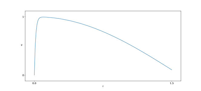
Figure 3. Numerical solution of a stiff ordinary differential equation obtained by solving the nonlinear systems using the complex-step Newton method

First we solve the initial value problem $y^{\prime}(t)=f(y(t),t)$ with $y(0)=0$ and $f(y,t)=-50(y-\cos~{}t)$. This is a stiff ordinary differential equation where its numerical approximation requires appropriate numerical methods.

In this experiment we took $\Delta t=10^{-2}$ and for $h=1/n$ for $n=1,2,\dots,10^{6}$ we obtained the solution with extremely fast convergence that required $2$ iterations for all values of $h$ and for all stages of the Runge-Kutta method indicating high-order convergence rate. At every iteration we used the solution of the previous step as an initial condition for the next complex-step Newton iteration. The tolerance we used for this case was $10^{-15}$ for determining the convergence of the Newton method and $10^{-25}$ for the convergence of the GMRES method.

We also considered a 4D dynamical system known as Olsen model for biochemical peroxidase-oxidase reaction [12]. A characteristic property of this system is that one component of its solution varies much slower than the other three. The Olsen system

(31) $$\frac{dA}{dt} =\mu-\alpha A-ABY\ ,$$

$$\frac{dB}{dt} =\varepsilon(1-BX-ABY)\ ,$$

$$\frac{dX}{dt} =\lambda(BX-X^{2}+3ABY-\zeta X+\delta)\ ,$$

$$\frac{dY}{dt} =\kappa\lambda(X^{2}-Y-ABY)\ ,$$

where we used the parameters $\alpha=0.0912$, $\beta=1.2121\times 10^{-5}$, $\varepsilon=0.0037$, $\lambda=18.5281$, $\kappa=3.7963$, $\mu=0.9697$, $\zeta=0.9847$. This in combination with the initial conditions $(A(0),B(0),X(0),Y(0))=(1,1,1,1)$ leads to a spiral solution in the four-dimensional phase-space [11]. Taking $t\in[0,10]$ and $\Delta t=0.01$ we obtained the solution where its projection in the space $A-B-X$ is depicted in Figure 4. The particular solution was obtained with $h=0.1$ and tolerance for the complex-step Newton method $10^{-12}$. As it was expected, the complex-step Newton method converged within 4 iterations for all values of $h<1$ that we used. This verifies the theory presented in the previous section.

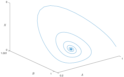
Figure 4. Projection of the heteroclinc orbit of the Olsen system in the space $A-B-X$

Solution of a complex system

Here we consider a more complicated example. Specifically, we demonstrate the ability of the complex-step Newton method to solve complex equations in a case of significant interest by solving the corresponding real and imaginary parts of the equations as real equations. In particular we consider the computation of ground states of the Discrete Nonlinear Schrödinger (DNLS) equation which is a system of complex nonlinear ordinary differential equations with applications in biology, optics, plasma physics and other fields of science. For more information about the particular equation we refer the interested reader to the book [8].

We consider the DNLS equation

(32) $$\mathrm{i}\dot{u}_{n}+(u_{n+1}-2u_{n}+u_{n-1})+|u_{n}|^{2}u_{n}=0\ ,$$

where $u_{n}=u_{n}(t):\mathbb{R}\to\mathbb{C}$ can be thought of as an approximate solution of the Nonlinear Schrödinger equation at the lattice sites $n=1,2,\dots,N+1$ with periodic boundary condition $u_{1}(t)=u_{N+1}(t)$. In the previous notation $\mathrm{i}=\sqrt{-1}$ and $\dot{u}_{n}=\tfrac{d}{dt}u_{n}(t)$. Solutions of the DNLS equation conserve the Hamiltonian

(33) $$H(t)=-\sum_{n=1}^{N}[|u_{n}-u_{n-1}|^{2}-\frac{1}{2}|u_{n}|^{4}]\ ,$$

and the norm

(34) $$P(t)=\sum_{n=1}^{N}|u_{n}|^{2}\ .$$

First we search for steady state solutions of the form $u_{n}=e^{\mathrm{i}\omega t}v_{n}$, where $\omega\in\mathbb{R}$ and $v_{n}\in\mathbb{C}$ independent of $t$. Substitution of this ansatz into the DNLS equation (32) yields a system of complex equations

(35) $$-\omega v_{n}+(v_{n+1}-2v_{n}+v_{n-1})+|v_{n}|^{2}v_{n}=0,\quad n=1,2,\dots,N\ .$$

Denoting $v_{n}=x_{n}+\mathrm{i}y_{n}$ we write the system (35) in the form $\mathbf{F}(\mathbf{x})=\mathbf{0}$ where $\mathbf{x}=(x_{1},\dots,x_{N},y_{1},\dots,y_{N})^{T}$ and $\mathbf{F}:\mathbb{R}^{2N}\to\mathbb{R}^{2N}$ with $\mathbf{F}(\mathbf{x})=(\mathbf{X}(\mathbf{x}),\mathbf{Y}(\mathbf{x}))^{T}$ where $\mathbf{X},\mathbf{Y}:\mathbb{R}^{N}\to\mathbb{R}^{N}$ are real vectors with entries

$$X_{j}=-\omega x_{j}+(x_{j+1}-2x_{j}+x_{j-1})+(x_{j}+y_{j})^{2}x_{j}\ ,$$

and

$$Y_{j}=-\omega y_{j}+(y_{j+1}-2y_{j}+y_{j-1})+(x_{j}^{2}+y_{j}^{2})y_{j}\ ,$$

for $j=1,2,\dots,N$. Note that in the previous expressions periodic boundary conditions must be employed for $j=1$ and $j=N$ so as the equations to make sense.

Setting the tolerance for convergence to be $\|\mathbf{x}^{(k+1)}-\mathbf{x}^{(k)}\|<10^{-13}$, $h$ as before, and taking a lattice with $N=200$ points we obtained the numerical ground state solution within 22 iterations independent of the choice of $h$. As initial guess of the solution we used the soliton-like profile

$$v_{n}^{(0)}=\frac{1+\mathrm{i}}{2}{\text{sech}}^{2}(n-n_{0})\ ,$$

where $n_{0}=100$. The computed solution is presented in Figure 5(a).

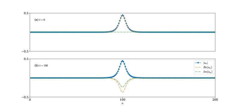
Figure 5. The numerical solution at $t=0$ and $t=100$

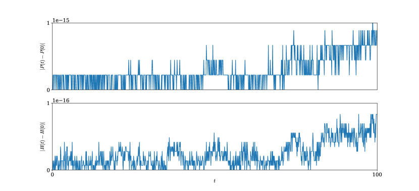
Figure 6. The error in the computed momentum and Hamiltonian

In order to further assess the convergence of the complex-step Newton iteration, we approximate numerically the solution of the DNLS equation with initial condition the numerically obtained ground state. For this reason we use again the fourth-order Gauss-Legendre Runge-Kutta method given by the tableau (29). This method has been studied for the numerical solution of the nonlinear Schrödinger equation in [5]. In order to apply the complex-step Newton method again we rewrite the complex system of differential equations into a system of real differential equations. In particular, if we denote $R_{n}=\mathrm{Re}(u_{n})$ and $I_{n}=\mathrm{Im}(u_{n})$ we write system (32) in the form

(36) $$\frac{d}{dt}R_{n} =-(I_{n+1}-2I_{n}+I_{n-1})-|u_{n}|^{2}I_{n}\ ,$$

$$\frac{d}{dt}I_{n} =R_{n+1}-2R_{n}+R_{n-1}+|u_{n}|^{2}R_{n}\ ,$$

and we approximate the solution of the nonlinear system (30) using the complex-step Newton method. For the discretization, we used a final time of $T=100$ and a time step of $\Delta t=0.1$. We tested the behaviour of the complex-step Newton method for various values of the complex complex-step $h\leq 1$, and we found that the method converged for all values we tried. Specifically, the complex-step Newton method converged within 4 iterations for all intermediate stages and for all values of $h$ we used, while we used the tolerance $10^{-15}$ for the convergence. For some values $h>1$ that we used we observed that the method didn’t converge. The solution at $t=100$ is presented in Figure 5(b). The momentum was preserved at the value $P=1.25217740216981$, while the Hamiltonian remained at $H=0.041394478363771$. These values indicate an error in momentum of the order $10^{-15}$ and an error of $10^{-16}$ in the Hamiltonian. The error in their computation is depicted in Figure 6. When we attempted initial conditions that did not correspond to traveling or standing waves, the solution preserved the momentum within machine precision, but the Hamiltonian was conserved to an order of $10^{-11}$. This aligns with the nearly preserved Hamiltonian of symplectic methods [2]. This is an indication that although the numerical method required approximation of solutions through iterative methods (GMRES and complex-step Newton methods), the results remained very accurate. For other application and examples we refer to [4].

4. Conclusions

In this work, we considered the Jacobian-free complex-step Newton method. After deriving the complex-step Newton iteration for both scalar and systems of equations, we proved its convergence. Specifically, we established that the convergence in the scalar case is linear, but it increases to quadratic as the complex-step parameter $h$ tends to zero. In the case of systems of equations the current method converges quadratically for any appropriately small value $h>0$. We concluded this work with experimental studies on the convergence of the complex-step iteration. We also tested the method against the numerical solution of a stiff ordinary differential equation with a symplectic Runge-Kutta method and we examined a discretization of the Nonlinear Schrödinger equation using the same symplectic method, which, aided by the complex-step Newton iteration, operated seamlessly.

References

• [1] M. Ablowitz and A. Fokas. Complex variables: Introduction and applications. Cambridge University Press, 2003.
• [2] E. Hairer, C. Lubich, and G. Wanner. Geometric numerical integration: Structure-preserving algorithms for ordinary differential equations. Springer-Verlag Berlin Heidelberg, 2006.
• [3] E. Hairer and G. Wanner. Solving ordinary differential equations II: Stiff and differential-algebraic problems. Springer-Verlag Berlin Heidelberg, 1996.
• [4] Z. Kan, N. Song, H. Peng, and B. Chen. Extension of complex step finite difference method to Jacobian-free Newton–Krylov method. Journal of Computational and Applied Mathematics, 399:113732, 2022.
• [5] O. Karakashian, G. Akrivis, and V. Dougalis. On optimal order error estimates for the nonlinear Schrödinger equation. SIAM Journal on numerical analysis, 30:377–400, 1993.
• [6] C. Kelley. Iterative method for linear and nonlinear equations. SIAM, Philadelphia, 1995.
• [7] C. Kelley. Newton’s method in mixed precision. SIAM Review, 64:191–211, 2022.
• [8] P. Kevrekidis. The Discrete Nonlinear Schrödinger Equation. Springer Berlin, Heidelberg, 2009.
• [9] D. Knoll and D. Keyes. Jacobian-free Newton–Krylov methods: a survey of approaches and applications. Journal of Computational Physics, 193:357–397, 2004.
• [10] J. Lyness and C. Moler. Numerical differentiation of analytic functions. SIAM Journal on Numerical Analysis, 4:202–210, 1967.
• [11] E. Musoke, B. Krauskopf, and H. Osinga. A surface of heteroclinic connections between two saddle slow manifolds in the Olsen model. International Journal of Bifurcation and Chaos, 30:2030048, 2020.
• [12] L. Olsen. An enzyme reaction with a strange attractor. Physics Letters A, 94(9):454–457, 1983.
• [13] J. Ortega. Numerical analysis: A second course. SIAM, Philadelphia, 1990.
• [14] J. Ortega and W. Rheinboldt. Iterative solution of nonlinear equations in several variables. SIAM, Philadelphia, 2000.
• [15] Y. Saad. Iterative methods for sparse linear systems. SIAM, Philadelphia, 2003.
• [16] J.M. Sanz-Serna and M.P. Calvo. Numerical Hamiltonian problems. Chapman and Hall/CRC Press, London, 1994.
• [17] W. Squire and G. Trapp. Using complex variables to estimate derivatives of real functions. SIAM review, 40:110–112, 1998.
• [18] J.L. Taylor. Foundations of Analysis. American Mathematical Society, 2012.