SAM-guided Graph Cut for 3D Instance Segmentation

Haoyu Guo^1∗ He Zhu^2∗† Sida Peng¹ Yuang Wang¹
Yujun Shen³ Ruizhen Hu⁴ Xiaowei Zhou¹
¹Zhejiang University ²Beijing Normal Univeristy ³Ant Group ⁴Shenzhen Univeristy

Abstract

This paper addresses the challenge of 3D instance segmentation by simultaneously leveraging 3D geometric and multi-view image information. Many previous works have applied deep learning techniques to 3D point clouds for instance segmentation. However, these methods often failed to generalize to various types of scenes due to the scarcity and low-diversity of labeled 3D point cloud data. Some recent works have attempted to lift 2D instance segmentations to 3D within a bottom-up framework. The inconsistency in 2D instance segmentations among views can substantially degrade the performance of 3D segmentation. In this work, we introduce a novel 3D-to-2D query framework to effectively exploit 2D segmentation models for 3D instance segmentation. Specifically, we pre-segment the scene into several superpoints in 3D, formulating the task into a graph cut problem. The superpoint graph is constructed based on 2D segmentation models, where node features are obtained from multi-view image features and edge weights are computed based on multi-view segmentation results, enabling the better generalization ability. To process the graph, we train a graph neural network using pseudo 3D labels from 2D segmentation models. Experimental results on the ScanNet, ScanNet++ and KITTI-360 datasets demonstrate that our method achieves robust segmentation performance and can generalize across different types of scenes. Our project page is available at https://zju3dv.github.io/sam_graph.

^†^†^∗Equal contribution. ^†Work done during internship at Zhejiang University.

1 Introduction

Refer to caption — Figure 1: Comparison of the generalization ability. By constructing superpoint graph with SAM [25], our 3D segmentation method demonstrates commendable generalizability. After training on ScanNet, not only do we achieve good performance on its validation set, but we can also effectively generalize to data collected with different devices (ScanNet++) and even to entirely different types of scenes (KITTI-360).

Instance segmentation of 3D scenes is a cornerstone of many applications, such as augmented and virtual reality, robot navigation, and autonomous driving. One typical pipeline for 3D scene segmentation is using deep neural networks[37, 38, 29, 48] to process the point cloud of the target scene to predict segmentation results. These methods[28, 11, 52, 56, 19, 12, 23, 50, 42] generally require annotated point clouds for training. However, annotating point clouds is costly, and there is a lack of datasets with the large scale and diversity similar to 2D image datasets. As a result, these methods are often limited to specific types of scenes and struggle to generalize to in-the-wild scenes.

Compared to point clouds, the acquisition and annotation of images are much less costly. In recent years, with the emergence of large-scale labeled 2D datasets and improvement in model architecture and capacity, state-of-the-art 2D instance segmentation models [25, 24, 4, 39] with strong generalization capabilities have been developed. Consequently, a natural approach of 3D segmentation is to lift multi-view 2D segmentations to 3D, leveraging them to achieve segmentation in arbitrary 3D scenes.

Recently, some 2D-to-3D lifting methods [57, 53, 54, 26, 44, 1, 58] have used a bottom-up framework, which first runs 2D segmentation on each view to obtain several masks, and then attempts to establish correspondences among masks across different views. These masks are then merged in 3D to obtain the 3D segmentation results. However, such bottom-up approach has a significant issue: 2D segmentation masks from different views may be inconsistent. For example, some instances may be segmented in some views but missing in others, thus severely degrading the performance of 3D segmentation.

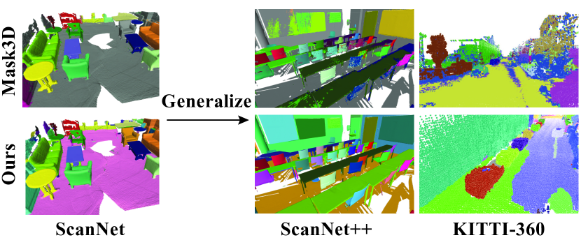
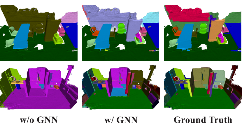
In this paper, we propose a novel 3D segmentation approach based on a 3D-to-2D query framework, which effectively utilizes 2D segmentation models. Unlike previous methods that generate multiple masks from multi-view images first, our approach begins with a pre-segmentation of the 3D scene into several superpoints. Then, we construct a superpoint graph of the target scene and transform the problem into graph segmentation. The edge weights of the graph are obtained by projecting graph nodes onto multiple views, using the prompt mechanism of SAM [25] to predict multi-view masks, and calculating the intersection of corresponding masks. The node features are obtained by aggregating multi-view image features. Finally, we use a graph neural network to regress the edge affinity for the graph partition [46]. The SAM-based graph enables better generalization ability, as shown in Fig. 1. In addition, we develop a scheme to generate pseudo 3D labels from a 2D segmentation network and design a training strategy to effectively leverages these pseudo labels, allowing us to train our model without any manual 3D annotations.

We conduct experiments on the ScanNet dataset, training the graph neural network on the training set and evaluating on the validation set, achieving state-of-the-art results. Without any fine-tuning, we also evaluate our method on ScanNet++ and KITTI-360 datasets. The experimental results indicate that, with the guidance of SAM in the construction of the graph, our method demonstrates excellent generalization capabilities. It can generalize across different types of data, encompassing different data acquisition methods and scene types.

In summary, our contributions are as follows:

•

We propose a novel 3D-to-2D-query framework that leverages SAM to construct node features and edge weights of the superpoint graph, effectively improving the generalization ability of the graph segmentation.
•

We develop a scheme to generate pseudo 3D labels from a 2D segmentation network, enabling our model to be trained without any manual 3D annotations.
•

We achieve robust segmentation results on ScanNet [6] and effectively generalize to ScanNet++ [59] and KITTI-360 [30] datasets.

2 Related work

3D scene segmentation.

The goal of 3D scene segmentation is to group the scene point cloud into semantically meaningful regions or distinct objects. Previous works leverage large-scale 3D labeled datasets to accomplish this objective in a supervised manner. They first train a neural network to extract per-point features, and then assign one predicted label to each point based on the extracted features. [16, 32, 21, 51, 47, 38, 29, 55, 48] achieve semantic segmentation on point cloud, and [28, 11, 52, 56, 19, 12, 23, 50] further distinguish between different objects with the same semantics, thus getting 3D instance segmentation results. Recently, Mask3D[42] leverage Transformer[49] to construct the segmentation network, attaining superior instance segmentation quality on 3D point clouds. 3D-SIS[20] performs 3D instance segmentation on RGB-D scan data, fusing image features extracted from 2D convolution networks with 3D scan geometry features, allowing accurate inference for object bounding boxes, class labels, and instance masks.

Some works exploit 2D large vision-language models to achieve open-vocabulary segmentation in 3D space. OpenScene[36] back-project per-pixel image features extracted by large vision language models from multi-view posed images to form a feature point cloud endowed with open-vocabularity abilities for various down-stream scene understanding tasks. PLA[10] constructs multi-scale 3D-text pairs and uses contracstive learning to enable the model to learn language-aware embeddings for 3D semantic and instance segmentation.

Partitioning 3D point cloud into a collection of small, geometrically homogeneous regions, coined superpoints, can yield a decent rough prediction and effectively simplify the process of scene segmentation. [45] and [22] propose to represent each 3D scene by constructing a superpoint graph, where superpoints serve as graph nodes, and then based on this graph, 3D instance segmentation is performed by learning inter-superpoint affinity and clustering superpoint nodes into 3D objects.

2D-to-3D lifting.

Due to the lower cost of acquiring and annotating 2D images, the scale and diversity of 2D annotated datasets [9, 31, 27, 5, 13, 18], are much larger compared to 3D datasets, facilitating the emergence of many highly effective 2D segmentation methods [25, 24, 39, 4] in recent years, making the use of 2D segmentation for 3D tasks a new and promising approach. Semantic-NeRF [61], based on the NeRF framework, utilizes outputs from a 2D semantic segmentation network at each view to train a 3D semantic field. Since it can fuse information from multiple viewpoints, this method is robust to inaccuracies and noise in individual view segmentations, yielding better 3D semantic segmentation results. However, extending this approach directly to instance segmentation is challenging, which is more complex since instance IDs in multi-view image segmentation results may not be consistent, making it necessary to design an effective label matching mechanisms in order to lift multi-view 2D instance segmentation results to 3D space.

To address this issue, [44] solves a linear assignment for instance identifiers across views with machine generated semantic and instance labels as supervision, [1] proposes a scalable slow-fast clustering objective function to fuse 2D predictions into a unified 3D scene segmentation results represented with a neural field, but they fail to produce satisfactory results for complex scenes with a large number of instances. SAD [2] uses SAM to segment both images and depth maps, combining the advantages of both for improved results. SAM3D [58] proposes a method for point cloud fusion. It segments each frame and gradually merges the segmentation results of all frames together. For scenes with known geometry, it can achieve segmentation very efficiently. Some works integrate SAM [25] into the Neural Radiance Fields (NeRF) [33] framework for 3D segmentation. For example, [3] merges SAM features into Instant NGP [34] in 3D, allowing users to segment an object from 3D space through multiple clicks. OR-NeRF [60] enables users to segment an object by clicking and then remove it from the scene.

Additionally, some methods combine segmentation and reconstruction, enabling separate reconstruction of each object. [57] propose to decompose a scene by learning an object-compositional nerual radiance field, with each standalone object separated from the scene and encoded with a learnable object activation codes, allowing more flexible downstream applications. To cope with the ambiguity of conventional volume rendering pipelines, [53, 54] further utilizes the Signed Distance Function (SDF) representation to exert explicit surface constraint.[26] represents each object in the scene with a small MLP and builds an object-level dense SLAM that detects objects on-th-fly and dynamically adds them to its map.

3 Method

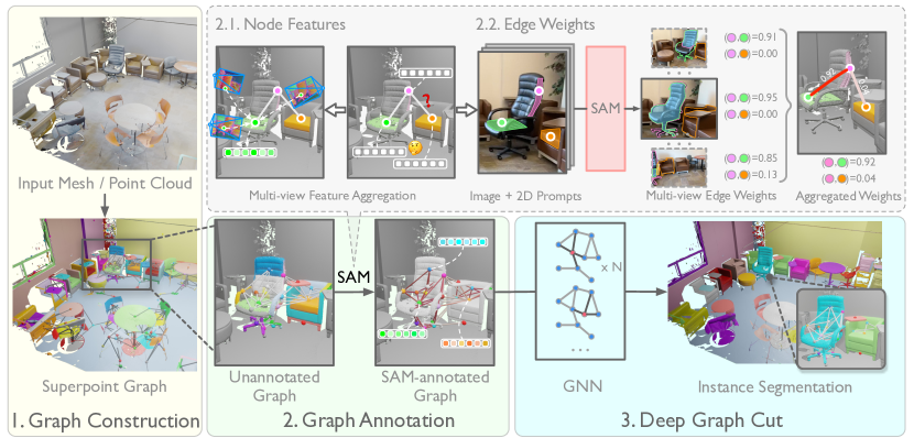
Given 3D geometry and calibrated multi-view images of a scene, our goal is to obtain the 3D instance segmentation of the scene. In this paper, we propose a novel segmentation framework, as illustrated in Fig. 2. We first perform over-segmentation on the 3D geometry to generate a set of superpoints, reformulating the task into a graph cut problem (Sec. 3.1). Then, Sec. 3.2 describes how to leverage SAM to construct node features and edge weights of the superpoint graph. In Sec. 3.3, we introduce a graph neural network for 3D segmentation, which is trained with pseudo labels generated by 2D segmentation predictions.

3.1 Building the superpoint graph

In an indoor or outdoor scene, not only can we easily acquire multi-view images, but we can also obtain the scene’s geometry (either in point clouds or mesh form) through depth cameras/laser scanners (for indoor scenes) or lidar (for large-scale outdoor scenes). With the geometry of the scene available, we can proceed to pre-segment the scene based on traditional methods to obtain a set of superpoints. For mesh, we apply the method in [6], which calculating the similarity between mesh vertices based on their normal directions and then conduct the graph cut algorithm [14]. For point clouds, we employ the method in [17], which first compute a local geometric feature vector (dimensionality and verticality) for each point, then perform Potts energy segmentation [8].

We can formulate the scene’s instance segmentation task as a graph cut problem by employing superpoints. Specifically, we first represent the scene as a graph $G=(V,E)$ , where $V$ denotes the set of superpoints in the scene and $E$ denotes the adjacency relationships between these superpoints. Two superpoints are considered as adjacent if their distance is within a predefined threshold. By employing superpoints, we can simplify the segmentation task in two ways. Firstly, the number of superpoints is substantially lower than the number of points in the original point cloud. Secondly, superpoints serve as a 3D proxy, enabling us to utilize multi-view image information and SAM’s prompt mechanism to determine the connection between regions in 3D space.

3.2 Constructing edge weights and node features

To accomplish segmentation of the 3D scene, our primary task is to determine whether two superpoints on each edge in graph should be merged. To this end, we leverage multi-view image information and employ SAM to annotate the graph so that we can send the annotated graph into neural network for segmentation. Specifically, we utilize the prompt mechanism of SAM to annotate the edges and use SAM encoder features to annotate the nodes.

Prompt mechanism of SAM.

Unlike previous 2D instance segmentation methods that take an image as input and output its segmentation map, SAM (Segment Anything Model) [25] operates by taking an image and a prompt as inputs and producing corresponding segmentation result. A typical prompt could be one or several 2D points. The image and the prompt are fed into an image encoder and a prompt encoder separately. Subsequently, a transformer-based decoder computes the cross-attention between prompt features and image features to generate the mask. Specifically, SAM can output multiple valid masks with associated confidence scores. In our experiments, we tend to prefer masks with a larger area because they are more likely to represent an entire object. We only resort to selecting masks with a relatively smaller area when the confidence of the larger mask is low (please refer to the supplementary materials for detailed implementation).

Edge weights.

The prompt mechanism of SAM introduces flexibility to calculate the edge weights between two 3D superpoints. Part 2.2 of Fig. 2 presents an illustration of computing the weight. Specifically, we first select a view where both superpoints are visible (if such a view does not exist, we regard the weight to be zero). Then, the two superpoints are projected onto the image space and $k$ points are uniformly sampled in each projection to serve as prompts for running SAM, thereby obtaining a mask for each superpoint. For masks corresponding to the two superpoints, we examine their intersection situation. Specifically, if two superpoints of an edge correspond to masks $A$ and $B$ , then we calculate the edge weight as $w=\max(\frac{A\bigcap B}{A},\frac{A\bigcap B}{B})$ , where $A\bigcap B$ denotes the intersection of $A$ and $B$ .

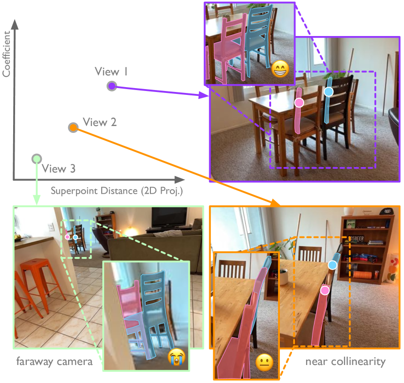
Taking into account that two superpoints may be co-visible in multiple views, we calculate edge weights estimation across all these views and take their weighted average: $w=\sum_{i}c_{i}w_{i}$ , where $w_{i}$ is the edge weight estimation of view $i$ and $c_{i}$ is the corresponding coefficient. $c_{i}$ is computed based on the following two factors: first, we consider the confidence of the two masks predicted by the SAM network; then, we consider the distance between the projections of the two superpoints in that view, as illustrated in Fig. 3. Specifically, for a view, we obtain its score by multiplying the 2D distance of two superpoints with the confidence of two corresponding masks. Then, we perform L1 normalization to multi-view scores to obtain coefficient $c_{i}$ for each view.

Node features.

In addition to edge weights, we also annotate node features with SAM. Specifically, for each node in the graph model, we identify all views that observe the corresponding superpoint. Within the projection range of that superpoint in each view, we randomly sample several points, interpolate to obtain features extracted by the SAM encoder and average the features obtained from all views to represent the attributes of that vertex. Part 2.1 of Fig. 2 presents an example of obtaining node features.

3.3 Deep graph cut

The edge weights calculated in Sec. 3.2 can be used to assess the affinity between two superpoints. While it’s possible to perform graph cut based directly on these weights, there is a drawback with this approach that can lead to suboptimal results: the calculation of each edge’s affinity is independent, lacking a global perspective, which maybe harmful for the final results. For instance, consider two objects composed of superpoints sets $A$ and $B$ , interconnected by $n$ edges. Even if most of these edges are correctly predicted to have low affinity, the erroneous high affinity prediction of just one edge can result in the incorrect segmentation of objects $A$ and $B$ together. To improve the robustness of segmentation and reduce the occurrence of such situations, we feed the graph model into a graph neural network (GNN), which has a certain receptive field and can utilize the information of the surrounding nodes and edges.

We utilize the GNN to predict affinity scores of graph edges, which are fed into the graph cut algorithm for 3D segmentation. To process the input graph, we design a GNN that consists of graph convolutional layers and fully connected layers. The graph model is first passed through graph convolutional layers to extract features for each vertex. Then, we concatenate features of two vertices with the corresponding edge score computed in Sec. 3.2, which are fed into fully connected layers to predict the affinity between two vertices.

When performing inference on a scene, we first utilize the trained GNN to predict the affinity scores of all edges in the graph, and then we segment the graph according to the affinity scores. Then we perform graph cut to cut the edges with low affinity score and then cluster the connected vertices as the final segmentation result, please refer to Sec. 4 for implementation details.

Pseudo labels generation.

We propose a strategy for training the GNN without 3D ground truth annotation. To supervise the network, we first generate pseudo labels based on a 2D segmentation model. For pseudo-labels, the most ideal case would be to obtain the correct affinity for all edges, but this is unrealistic. In fact, while we require a high degree of accuracy for pseudo-labels, the completeness of these labels is a lesser priority. For this purpose, we use a 2D segmentation network, CropFormer [39], for this task. We first ran CropFormer on all views to obtain the instance segmentation results. For each pair of co-visible superpoints in every view, we record whether these superpoints are within the same mask. If they are co-visible in at least $n$ views and their records are consistent across all these n views, then we treat the pair as a pseudo-label. For example, if two superpoints are within the same mask in all co-visible views, they are treated as a positive sample in the pseudo-labels, vice versa.

The reason for the choice is based on our empirical observation that CropFormer tends to yield relatively more complete and accurate masks for common object categories. For example, CropFormer consistently segments a chair entirely, whereas SAM sometimes segments parts of it, such as a single chair leg. Although CropFormer has its advantages, we opt for SAM in the previous graph construction stage due to the following considerations: Due to SAM’s unique prompt mechanism, it can use superpoints to control the granularity of segmentation to some extent. Moreover, SAM’s design, which allows for predicting multiple masks from a single prompt, makes it more adept at handling uncommon objects. Consequently, we chose SAM for constructing the entire graph, while using CropFormer to generate relatively incomplete but high-quality pseudo-labels.

Training of the GNN.

We employ pseudo-labels generated by CropFormer as supervision. For the edges included in these pseudo-labels, we compare the affinity scores of these edges predicted by GNN with the labels to binary cross-entropy loss, which is defined as

L_{\text{BCE}}=s_{\text{ps}}\log(s)+(1-s_{\text{ps}})\log(1-s),

(1)

where $s$ is the predicted affinity score and $s_{\text{ps}}$ is the pseudo-label of corresponding edge. Since pseudo-labels are sparse, we observed that direct training in this manner tends to limit the network’s capabilities. To improve the accuracy of the graph network’s predictions, we introduce an additional regularization for edges not included in the pseudo-labels during training. This regularization aims to ensure the predicted affinity score $s$ , and the edge weight predicted by SAM, $w_{\text{SAM}}$ , to be as consistent as possible. This loss is defined as

L_{\text{reg}}=|w_{\text{SAM}}-0.5|L_{1}(s,w_{\text{SAM}}).

(2)

With this design, the closer $w_{\text{SAM}}$ is to 0 or 1, the greater the penalty for inconsistency between $s$ and $w_{\text{SAM}}$ .

4 Implementation details

Graph construction.

When sampling points within the projection of a superpoint as prompts for SAM, we uniformly sample $k=5$ points within the projected mask. Considering that there might be slight inaccuracies in the camera poses, the points too close to the boundaries of projection masks could potentially fall outside the object. Therefore, we take care to avoid sampling these points during this process.

	ScanNet			ScanNet++			KITTI-360
	mAP	AP₅₀	AP₂₅	mAP	AP₅₀	AP₂₅	mAP	AP₅₀	AP₂₅
Felzenswalb	1.9	5.8	22.9	5.8	12.4	29.7	-	-	-
Guinard	0.6	2.4	24.0	0.8	2.8	16.5	2.1	6.2	24.1
SAM3D (w/o ensemble)	6.3	17.9	47.3	1.7	5.4	20.9	2.5	7.5	22.4
SAM3D (w/ ensemble)	13.7	29.7	54.5	8.3	17.5	33.7	6.3	16.0	35.6
SAM-based Graph + NCuts	5.1	13.6	39.5	7.5	16.5	34.2	10.1	18.4	31.0
SAM-based Graph + DBSCAN	6.6	14.1	24.7	8.2	15.0	22.6	12.9	23.5	35.6
SAM-based Graph + Graph partition	12.9	30.0	57.7	12.6	24.5	40.2	12.6	25.5	41.9
Ours	15.1	33.3	59.1	12.9	25.3	43.6	14.7	28.0	43.2

Table 1: Quantitative results of 3D segmentation on ScanNet, ScanNet++ and KITTI-360 datasets. We report the AP scores averaged on all test scenes. Our method significantly outperforms the baseline methods on all datasets.

Training and inference of GNN.

We implement the GNN with PyTorch [35] and PyG [15]. When generating pseudo labels with CropFormer, we only consider the superpoint pairs that are co-visible in at least $n=10$ views with all consistent records. We train the GNN on ScanNet for 200 epochs, which takes about 20 minutes on NVIDIA A6000 GPU.

When performing segmentation based on the output of GNN, for every two vertices, if their affinity is below a certain threshold, we consider them to be unconnected. Conversely, if their affinity is above this threshold, to further improve robustness, we identify paths of length 2 between these two vertices. We then record the number of paths where both edges have high affinity scores and the number where one edge is high and the other low. If the ratio of the latter exceeds a predefined threshold, we regard the two vertices to be unconnected; otherwise, they are considered as connected. Once the connection status of each edge is determined using this method, we employ a union-find algorithm [46] to merge all connected superpoints, resulting in the 3D segmentation of the scene.

5 Experiments

5.1 Datasets, metrics and baselines

Datasets.

We perform the experiments on ScanNet (V2) [6], ScanNet++ [59] and KITTI-360 [30]. ScanNet is a large-scale RGB-D dataset that contains 1613 indoor scenes with geometry acquired by BundleFusion [7] and images captured by iPad Air2. ScanNet++ contains 280 indoor scenes with high-fidelity geometry acquired by the Faro Focus Premium laser scanner as well as high-resolution RGB images captured by iPhone 13 Pro and a DSLR camera with a fisheye lens. KITTI-360 is a large outdoor dataset with 300 suburban scenes, which consists of 320k images and 100k laser scans obtained through a mobile platform in a driving distance of 73.7km. Both these datasets are annotated with ground truth camera poses and instance-level semantic segmentations. We train the GNN on 1201 training scenes of ScanNet, we then evaluate our method on 312 validation scenes of ScanNet, 50 of ScanNet++ and 61 scenes of KITTI-360, according to the official split of each dataset.

Metrics.

We evaluate ours segmentation performance with the widely-used Average Precision (AP) score. We follow the standard defined in [40, 6] for evaluation, calculating AP with thresholds of $50\%$ and $25\%$ (denoted as AP₅₀ and AP₂₅, respectively) as well as AP averaged with IoU thresholds from $50\%$ to $95\%$ with a step size of $5\%$ (mAP). Since our method as well as most of baseline methods are class-agnostic, we do not consider semantic class label in evaluation. Additionally, considering that some regions in the datasets lack instance annotations (such as come objects in ScanNet and trees in KITTI-360), unlike supervised training methods that can learn relevant priors from the annotations in the training set, our method as well as most baseline methods segment the entire scene. To facilitate a fairer comparison, we exclude the instances in unannotated regions during evaluation.

		mAP	AP ${}_{\text{50}}$	AP ${}_{\text{25}}$
ScanNet	Mask3D	26.9	44.4	57.5
ScanNet	Ours	19.0	38.9	59.9
ScanNet++	Mask3D	8.8	15.0	22.3
ScanNet++	Ours	14.3	26.7	43.5
KITTI-360	Mask3D	0.1	0.4	4.2
KITTI-360	Ours	14.7	28.0	43.2

Table 2: Comparison with Mask3D. While Mask3D shows slightly better performance than ours on ScanNet, when comparing generalization results on ScanNet++ and KITTI-360, our method significantly outperforms Mask3D.

Baselines.

We compare our method with the following baselines: (1) Traditional segmentation method: [14, 17], which use purely geometric information to perform segmentation. (2) 2D-to-3D lifting method: SAM3D [58] and Panoptic Lifting [44]. We report the results of SAM3D with and without ensemble process. Since Panoptic Lifting is based on NeRF [33] and requires hours for per-scene optimization, we only report corresponding qualitative analyses. (3) Point cloud segmentation method: Mask3D [42], we use their official pretrained model which is trained on ScanNet dataset. (4) We segment our SAM annotated graph (without GNN) with traditional spectral clustering methods: Normalized Cuts [43] and DBSCAN [41], as well as the graph cut used in our method.

5.2 Comparisons with the state-of-the-art methods

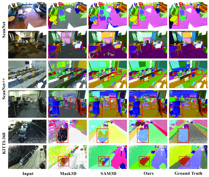
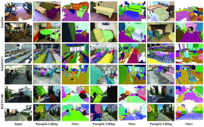
We evaluate 3D segmentation metrics on ScanNet, ScanNet++ and KITTI-360 datasets. Averaged quantitative results are shown in Tab. 1. We also provide qualitative results in Fig. 4. By analysing quantitative and qualitative results, we found that our method significantly outperforms state-of-the-art unsupervised methods.

Panoptic Lifting can achieve reasonably good segmentation results in simpler scenes, but its performance deteriorates in more complex environments with a large number of objects. SAM3D can handle complex scenes, however, its segmentation often results in both large structures, like floors, and smaller objects, like chairs, being divided into multiple segments. In contrast, our method is able to produce more accurate and complete segmentation results. In our experiments with Normalized Cuts and DBSCAN, we found that carefully tuning hyperparameters can yield good result for a single scene. However, each scene varies significantly in scale and the number of objects, leading to considerable differences in the optimal hyperparameters. When we apply uniform hyperparameters across all dataset, the averaged metrics are not ideal.

Comparisons with Mask3D

In addition to unsupervised baselines, we also compare our method with Mask3D, which is the state-of-the-art supervised learning method. When evaluation, we use the official pretrained model provided by Mask3D, which is trained on ScanNet dataset with GT annotations. For fair comparison, we ignore floor and wall regions when evaluating on ScanNet and ScanNet++ datasets. The quantitative results are shown in Tab. 2. The results show that our method achieve much better generalization performance.

	mAP	AP₅₀	AP₂₅
w/o GNN	12.9	30.0	57.7
w/o node features	13.4	30.7	58.0
w/o edge weights	1.9	5.6	22.0
w/o regularization loss	9.1	20.2	39.9
our full method	15.1	33.3	59.1

Table 3: Ablation studies on ScanNet dataset.

	Accuracy	Precision	Recall	F1-Score
SAM	0.892	0.934	0.888	0.911
CropFormer	0.912	0.934	0.923	0.929

Table 4: Analyses of the choice for pseudo-labels generation.

5.3 Ablation studies

We conduct ablation studies on ScanNet to show the effectiveness of each component and design. We evaluate with five configurations: (1) We directly use the edge weight of SAM annotated graph (without GNN) to apply graph cut. (2) We annotate the graph without node features. (3) We annotate the graph without edge weights. (4) We train GNN without regularization loss. (5) Our full method. We report the quantitative results in Tab. 3.

The results indicate that the absence of a GNN leads to a decline in segmentation performance. The most common issue is that some objects or structures are incorrectly connected together, as demonstrated by the examples in Fig. 5. Node features have a certain impact on the predictive performance of the GNN, while edge weights have a very significant impact, almost playing a dominant role. Additionally, we found that regularization loss is also very important.

Furthermore, we conducted experiments to analyse the advantages of using CropFormer to generate pseudo-labels compared to SAM. For the labels generated by CropFormer, we also used SAM to predict a label. The accuracy of both methods was evaluated using the ground truth annotations provided by ScanNet. As indicated in the Tab. 4, CropFormer achieved higher accuracy.

6 Conclusion

In this paper, we introduced a novel 3D segmentation method with SAM guided graph cut. The key idea is to pre-segment 3D scenes into superpoints, and then utilize the prompt mechanism of SAM to assess the affinity scores between superpoints. We propose a GNN based graph cut method to improve the robustness, which is trained with pseudo-labels generated by 2D segmentation network. Experiments showed that the proposed method was able to achieve accurate segmentation results and can generalize well to different datasets.

Discussion.

Our method not only requires geometric data (mesh/point cloud) but also needs multi-view images as input, which to some extent limits its application scenarios. Moreover, we perform segmentation based on merging SuperPoint. When an object is part of a SuperPoint, we are unable to segment it out. This situation occurs occasionally, for example, a poster adhered to a wall. To address this, a more sophisticated pre-segmentation model, which consider not only geometric information but also semantics, should be designed. One viable approach is to also use the guidance from SAM or other visual models during the pre-segmentation stage. We leave it to future works.

References

Bhalgat et al. [2023] Yash Bhalgat, Iro Laina, João F Henriques, Andrew Zisserman, and Andrea Vedaldi. Contrastive lift: 3d object instance segmentation by slow-fast contrastive fusion. arXiv preprint arXiv:2306.04633, 2023.
Cen et al. [2023] Jun Cen, Yizheng Wu, Kewei Wang, Xingyi Li, Jingkang Yang, Yixuan Pei, Lingdong Kong, Ziwei Liu, and Qifeng Chen. Sad: Segment any rgbd. arXiv preprint arXiv:2305.14207, 2023.
Chen et al. [2023] Xiaokang Chen, Jiaxiang Tang, Diwen Wan, Jingbo Wang, and Gang Zeng. Interactive segment anything nerf with feature imitation. arXiv preprint arXiv:2305.16233, 2023.
Cheng et al. [2022] Bowen Cheng, Ishan Misra, Alexander G Schwing, Alexander Kirillov, and Rohit Girdhar. Masked-attention mask transformer for universal image segmentation. In CVPR, 2022.
Cordts et al. [2016] Marius Cordts, Mohamed Omran, Sebastian Ramos, Timo Rehfeld, Markus Enzweiler, Rodrigo Benenson, Uwe Franke, Stefan Roth, and Bernt Schiele. The cityscapes dataset for semantic urban scene understanding. In CVPR, 2016.
Dai et al. [2017a] Angela Dai, Angel X Chang, Manolis Savva, Maciej Halber, Thomas Funkhouser, and Matthias Nießner. Scannet: Richly-annotated 3d reconstructions of indoor scenes. In CVPR, 2017a.
Dai et al. [2017b] Angela Dai, Matthias Nießner, Michael Zollhöfer, Shahram Izadi, and Christian Theobalt. Bundlefusion: Real-time globally consistent 3d reconstruction using on-the-fly surface reintegration. ACM ToG, 2017b.
Dann et al. [2012] Christoph Dann, Peter Gehler, Stefan Roth, and Sebastian Nowozin. Pottics–the potts topic model for semantic image segmentation. In Pattern Recognition. Springer, 2012.
Deng et al. [2009] Jia Deng, Wei Dong, Richard Socher, Li-Jia Li, Kai Li, and Li Fei-Fei. Imagenet: A large-scale hierarchical image database. In CVPR, 2009.
Ding et al. [2023] Runyu Ding, Jihan Yang, Chuhui Xue, Wenqing Zhang, Song Bai, and Xiaojuan Qi. Pla: Language-driven open-vocabulary 3d scene understanding. In CVPR, 2023.
Elich et al. [2019] Cathrin Elich, Francis Engelmann, Theodora Kontogianni, and Bastian Leibe. 3D-BEVIS: Birds-Eye-View Instance Segmentation. In The German Conference on Pattern Recognition, 2019.
Engelmann et al. [2020] Francis Engelmann, Martin Bokeloh, Alireza Fathi, Bastian Leibe, and Matthias Nießner. 3D-MPA: Multi Proposal Aggregation for 3D Semantic Instance Segmentation. In CVPR, 2020.
Everingham et al. [2015] M. Everingham, S. M. A. Eslami, L. Van Gool, C. K. I. Williams, J. Winn, and A. Zisserman. The pascal visual object classes challenge: A retrospective. IJCV, 2015.
Felzenszwalb and Huttenlocher [2004] Pedro F Felzenszwalb and Daniel P Huttenlocher. Efficient graph-based image segmentation. IJCV, 2004.
Fey and Lenssen [2019] Matthias Fey and Jan E. Lenssen. Fast graph representation learning with PyTorch Geometric. In ICLR Workshop on Representation Learning on Graphs and Manifolds, 2019.
Graham et al. [2018] Benjamin Graham, Martin Engelcke, and Laurens van der Maaten. 3D Semantic Segmentation with Submanifold Sparse Convolutional Networks. In CVPR, 2018.
Guinard et al. [2017] Stéphane Guinard, Loic Landrieu, and Bruno Vallet. Weakly supervised segmentation-aided classification of urban scenes from 3d lidar point clouds. 2017.
Gupta et al. [2019] Agrim Gupta, Piotr Dollar, and Ross Girshick. Lvis: A dataset for large vocabulary instance segmentation. In CVPR, 2019.
Han et al. [2020] Lei Han, Tian Zheng, Lan Xu, and Lu Fang. OccuSeg: Occupancy-aware 3D Instance Segmentation. In CVPR, 2020.
Hou et al. [2019] Ji Hou, Angela Dai, and Matthias Nießner. 3D-SIS: 3D Semantic Instance Segmentation of RGB-D Scans. In CVPR, 2019.
Huang and You [2016] Jing Huang and Suya You. Point Cloud Labeling Using 3D Convolutional Neural Network. In ICPR, 2016.
Hui et al. [2022] Le Hui, Linghua Tang, Yaqi Shen, Jin Xie, and Jian Yang. Learning superpoint graph cut for 3d instance segmentation. In NeurIPS, 2022.
Jiang et al. [2020] Li Jiang, Hengshuang Zhao, Shaoshuai Shi, Shu Liu, Chi-Wing Fu, and Jiaya Jia. PointGroup: Dual-Set Point Grouping for 3D Instance Segmentation. In CVPR, 2020.
Ke et al. [2023] Lei Ke, Mingqiao Ye, Martin Danelljan, Yifan Liu, Yu-Wing Tai, Chi-Keung Tang, and Fisher Yu. Segment anything in high quality. arXiv preprint arXiv:2306.01567, 2023.
Kirillov et al. [2023] Alexander Kirillov, Eric Mintun, Nikhila Ravi, Hanzi Mao, Chloe Rolland, Laura Gustafson, Tete Xiao, Spencer Whitehead, Alexander C. Berg, Wan-Yen Lo, Piotr Dollár, and Ross Girshick. Segment anything. In ICCV, 2023.
Kong et al. [2023] Xin Kong, Shikun Liu, Marwan Taher, and Andrew J Davison. vmap: Vectorised object mapping for neural field slam. In CVPR, 2023.
Krishna et al. [2017] Ranjay Krishna, Yuke Zhu, Oliver Groth, Justin Johnson, Kenji Hata, Joshua Kravitz, Stephanie Chen, Yannis Kalantidis, Li-Jia Li, David A Shamma, et al. Visual genome: Connecting language and vision using crowdsourced dense image annotations. IJCV, 2017.
Lahoud et al. [2019] Jean Lahoud, Bernard Ghanem, Marc Pollefeys, and Martin R. Oswald. 3D Instance Segmentation via Multi-task Metric Learning. In CVPR, 2019.
Li et al. [2018] Yangyan Li, Rui Bu, Mingchao Sun, Wei Wu, Xinhan Di, and Baoquan Chen. PointCNN: Convolution on X-transformed Points. In NeurIPS, 2018.
Liao et al. [2022] Yiyi Liao, Jun Xie, and Andreas Geiger. Kitti-360: A novel dataset and benchmarks for urban scene understanding in 2d and 3d. PAMI, 2022.
Lin et al. [2014] Tsung-Yi Lin, Michael Maire, Serge Belongie, James Hays, Pietro Perona, Deva Ramanan, Piotr Dollár, and C Lawrence Zitnick. Microsoft coco: Common objects in context. In ECCV, 2014.
Long et al. [2015] Jonathan Long, Evan Shelhamer, and Trevor Darrell. Fully Convolutional Networks for Semantic Segmentation. In CVPR, 2015.
Mildenhall et al. [2020] Ben Mildenhall, Pratul P. Srinivasan, Matthew Tancik, Jonathan T. Barron, Ravi Ramamoorthi, and Ren Ng. Nerf: Representing scenes as neural radiance fields for view synthesis. In ECCV, 2020.
Müller et al. [2022] Thomas Müller, Alex Evans, Christoph Schied, and Alexander Keller. Instant neural graphics primitives with a multiresolution hash encoding. ACM ToG, 2022.
Paszke et al. [2019] Adam Paszke, Sam Gross, Francisco Massa, Adam Lerer, James Bradbury, Gregory Chanan, Trevor Killeen, Zeming Lin, Natalia Gimelshein, Luca Antiga, et al. Pytorch: An imperative style, high-performance deep learning library. NeurIPS, 2019.
Peng et al. [2023] Songyou Peng, Kyle Genova, Chiyu ”Max” Jiang, Andrea Tagliasacchi, Marc Pollefeys, and Thomas Funkhouser. OpenScene: 3D Scene Understanding with Open Vocabularies. In CVPR, 2023.
Qi et al. [2017a] Charles R. Qi, Hao Su, Kaichun Mo, and Leonidas J. Guibas. PointNet: Deep Learning on Point Sets for 3D Classification and Segmentation. In CVPR, 2017a.
Qi et al. [2017b] Charles R. Qi, Li Yi, Hao Su, and Leonidas J. Guibas. PointNet++: Deep Hierarchical Feature Learning on Point Sets in a Metric Space. In NeurIPS, 2017b.
Qi et al. [2023] Lu Qi, Jason Kuen, Tiancheng Shen, Jiuxiang Gu, Wenbo Li, Weidong Guo, Jiaya Jia, Zhe Lin, and Ming-Hsuan Yang. High quality entity segmentation. In ICCV, 2023.
Ren et al. [2015] Shaoqing Ren, Kaiming He, Ross Girshick, and Jian Sun. Faster r-cnn: Towards real-time object detection with region proposal networks. In NeurIPS, 2015.
Schubert et al. [2017] Erich Schubert, Jörg Sander, Martin Ester, Hans Peter Kriegel, and Xiaowei Xu. Dbscan revisited, revisited: why and how you should (still) use dbscan. ACM Transactions on Database Systems (TODS), 2017.
Schult et al. [2022] Jonas Schult, Francis Engelmann, Alexander Hermans, Or Litany, Siyu Tang, and Bastian Leibe. Mask3d for 3d semantic instance segmentation. arXiv preprint arXiv:2210.03105, 2022.
Shi and Malik [2000] Jianbo Shi and Jitendra Malik. Normalized cuts and image segmentation. PAMI, 2000.
Siddiqui et al. [2023] Yawar Siddiqui, Lorenzo Porzi, Samuel Rota Bulò, Norman Müller, Matthias Nießner, Angela Dai, and Peter Kontschieder. Panoptic lifting for 3d scene understanding with neural fields. In CVPR, 2023.
Tang et al. [2022] Linghua Tang, Le Hui, and Jin Xie. Learning inter-superpoint affinity for weakly supervised 3d instance segmentation. In ACCV, 2022.
Tarjan [1975] Robert Endre Tarjan. Efficiency of a good but not linear set union algorithm. Journal of the ACM (JACM), 1975.
Tchapmi et al. [2017] Lyne P. Tchapmi, Christopher B. Choy, Iro Armeni, JunYoung Gwak, and Silvio Savarese. SEGCloud: Semantic Segmentation of 3D Point Clouds. In 3DV, 2017.
Thomas et al. [2019] Hugues Thomas, Charles R. Qi, Jean-Emmanuel Deschaud, Beatriz Marcotegui, François Goulette, and Leonidas J. Guibas. KPConv: Flexible and Deformable Convolution for Point Clouds. In ICCV, 2019.
Vaswani et al. [2017] Ashish Vaswani, Noam Shazeer, Niki Parmar, Jakob Uszkoreit, Llion Jones, Aidan N Gomez, Łukasz Kaiser, and Illia Polosukhin. Attention Is All You Need. In NeurIPS, 2017.
Vu et al. [2022] Thang Vu, Kookhoi Kim, Tung M. Luu, Xuan Thanh Nguyen, and Chang D. Yoo. SoftGroup for 3D Instance Segmentation on 3D Point Clouds. In CVPR, 2022.
Wang et al. [2015] Tianyi Wang, Jian Li, and Xiangjing An. An Efficient Scene Semantic Labeling Approach for 3D Point Cloud. In IEEE International Conference on Intelligent Transportation Systems (ITSC), 2015.
Wang et al. [2018] Weiyue Wang, Ronald Yu, Qiangui Huang, and Ulrich Neumann. SGPN: Similarity Group Proposal Network for 3D Point Cloud Instance Segmentation. In CVPR, 2018.
Wu et al. [2022] Qianyi Wu, Xian Liu, Yuedong Chen, Kejie Li, Chuanxia Zheng, Jianfei Cai, and Jianmin Zheng. Object-compositional neural implicit surfaces. In ECCV, 2022.
Wu et al. [2023] Qianyi Wu, Kaisiyuan Wang, Kejie Li, Jianmin Zheng, and Jianfei Cai. Objectsdf++: Improved object-compositional neural implicit surfaces. In ICCV, 2023.
Xu et al. [2018] Yifan Xu, Tianqi Fan, Mingye Xu, Long Zeng, and Yu Qiao. SpiderCNN: Deep Learning on Point Sets with Parameterized Convolutional Filters. In ECCV, 2018.
Yang et al. [2019] Bo Yang, Jianan Wang, Ronald Clark, Qingyong Hu, Sen Wang, Andrew Markham, and Niki Trigoni. Learning Object Bounding Boxes for 3D Instance Segmentation on Point Clouds. In NeurIPS, 2019.
Yang et al. [2021] Bangbang Yang, Yinda Zhang, Yinghao Xu, Yijin Li, Han Zhou, Hujun Bao, Guofeng Zhang, and Zhaopeng Cui. Learning object-compositional neural radiance field for editable scene rendering. In ICCV, 2021.
Yang et al. [2023] Yunhan Yang, Xiaoyang Wu, Tong He, Hengshuang Zhao, and Xihui Liu. Sam3d: Segment anything in 3d scenes. arXiv preprint arXiv:2306.03908, 2023.
Yeshwanth et al. [2023] Chandan Yeshwanth, Yueh-Cheng Liu, Matthias Nießner, and Angela Dai. Scannet++: A high-fidelity dataset of 3d indoor scenes. In ICCV, 2023.
Yin et al. [2023] Youtan Yin, Zhoujie Fu, Fan Yang, and Guosheng Lin. Or-nerf: Object removing from 3d scenes guided by multiview segmentation with neural radiance fields. arXiv preprint arXiv:2305.10503, 2023.
Zhi et al. [2021] Shuaifeng Zhi, Tristan Laidlow, Stefan Leutenegger, and Andrew J Davison. In-place scene labelling and understanding with implicit scene representation. In ICCV, 2021.

Appendix

	ScanNet			ScanNet++			KITTI-360
	mAP	AP₅₀	AP₂₅	mAP	AP₅₀	AP₂₅	mAP	AP₅₀	AP₂₅
SAM-based Graph + NCuts	5.1	13.6	39.5	7.5	16.5	34.2	10.1	18.4	31.0
SAM-based Graph + DBSCAN	6.6	14.1	24.7	8.2	15.0	22.6	12.9	23.5	35.6
SAM-based Graph + Graph partition	12.9	30.0	57.7	12.6	24.5	40.2	12.6	25.5	41.9
SAM-based Graph + GNN + NCuts	8.9	21.5	47.7	8.0	16.9	32.4	8.9	16.4	29.4
SAM-based Graph + GNN + DBSCAN	7.1	15.0	26.4	8.3	15.3	23.4	13.3	23.9	36.0
SAM-based Graph + GNN + Graph partition	15.1	33.3	59.1	12.9	25.3	43.6	14.7	28.0	43.2

Table 5: Ablation studies of different graph cut methods.

Appendix A Points sampling in projection mask

To sample $k=5$ points uniformly and not too far from the boundary of the projection mask of each superpoint in each view, we first use the Euclidean Distance Transform to compute the distance from each pixel within the mask to its boundary, creating a distance map. We then select the point with the maximum value in the distance map to ensure it is near the center. To prevent subsequent sampled points from being too close to this first point, we set the values in the distance map within a certain area around this point to zero. This process is iteratively repeated for sampling the remaining points.

Appendix B Structure of GNN

The Graph Neural Network (GNN) in our method consists of a 5-layer Graph Convolutional Network (GCN) and a 3-layer Multi-Layer Perceptron (MLP). The GCN has an input channel size of 256, which corresponds to the channel size of the SAM features. It has a hidden layer width of 128 and an output channel size of 128. The MLP has an input channel size of 257, which includes the concatenated GCN features of two nodes and one edge weight. Its hidden layer width is 128, and it has an output channel size of 1, corresponding to the affinity score of an edge.

Appendix C Comparison with Panoptic Lifting

We observed that Panoptic Lifting struggles to extract satisfactory geometry, so we render the results of Panoptic Lifting in several views and visualize our method in nearby views for comparison. We show the results in Fig. 6.

Appendix D Analyses of different graph cut method

Based on the graph constructed using SAM, we tested segmenting the graph using normalized cuts, DBSCAN, and the direct graph partition method used in our approach, both with and without using the GNN (without means directly using edge weight). The comparison results are shown in the Tab. 5. From the results, it’s evident that the use of GNN generally improves most metrics for normalized cuts, while DBSCAN and the direct graph partition method show comprehensive improvements across all metrics. Furthermore, regardless of the use of GNN, the direct graph partition method consistently outperforms both normalized cuts and DBSCAN. Our analysis suggests that while normalized cuts and DBSCAN are adept at obtaining a rough segmentation for graphs with unreliable edge affinities, they are less capable of achieving finer segmentation results even when edge affinities are highly reliable.

Appendix E Discussions of SAM guidance

As shown in the ablation studies in our paper, both the node features and edge weights calculated based on SAM are effective for our method, with the edge weights being particularly crucial. To further analyse their effectiveness, we attempted to remove both and use PointNet++ to compute node features. Specifically, we utilized PointNet++ to extract features from the point cloud, averaging the features within a superpoint to serve as the node feature. We employed the same loss function as in our method and optimized the network parameters of both PointNet++ and the GNN simultaneously. We found that this approach resulted in very poor performance.