Topological entanglement entropy for torus knot bipartitions and the Verlinde-like formulas

Abstract

The topological Rényi and entanglement entropies depend on the bipartition of the manifold and the choice of the ground states. However, these entanglement quantities remain invariant under a coordinate transformation when the bipartition also undergoes the same transformation. In the context of topological quantum field theories, these coordinate transformations reduce to representations of the mapping class group on the manifold of the Hilbert space. We employ this invariant property of the Rényi and entanglement entropies under coordinate transformations for TQFTs in (2 + 1) dimensions on a torus with various bipartitions. By utilizing the replica trick and the surgery method to compute the topological Rényi and entanglement entropies, the invariant property results in Verlinde-like formulas. Furthermore, for the bipartition with interfaces as two non-intersecting torus knots, an $SL(2,\mathbb{Z})$ transformation can untwist the torus knots, leading to a simple bipartition with an effective ground state. This invariant property allows us to demonstrate that the topological entanglement entropy has a lower bound $-2\ln D$, where $D$ is the total quantum dimensions of the system.

1 Introduction

After the publication of seminal papers on Chern-Simon Theory TQFT1 ; TQFT2 , topological quantum field theories (TQFTs) have found applications in studying the properties of topologically ordered systems with a mass gap. Notable examples include the fractional quantum Hall effect FQH ; FQH2 ; FQH3 ; FQH4 , gapped quantum spin liquids SpinLiquid , quantum dimer models Dimer , and $p_{x}+ip_{y}$ superconductors px+ipy . TQFTs can be regarded as effective field theories for these systems, treating the mass gap as infinite. Under this stringent condition, all excitations become irrelevant, allowing us to focus solely on the ground states, which exhibit long-range entanglement. Due to these long-range entangled properties, the number of ground states depends on the topology of the manifold, leading to these systems being referred to as having topological orders TO .

The concept of topological entanglement entropy (TEE) was later introduced by TEE ; TEE2 as a diagnostic tool for discerning topological orders in two dimensions. The TEE of these systems can be written as $\alpha L+S_{\text{TEE}}$, where $\alpha L$ is a term proportional to the area of the entanglement interface Area and the $S_{\text{TEE}}$ is a negative term due to the topological constraints of these systems. Extensive computations of the TEE in various lattice models have substantiated its efficacy in characterizing topological orders TO1 ; TO2 ; TO3 ; TO4 ; TO5 .

Alternatively, the TEE can be directly computed using the Von-Neumann entropy within the framework of TQFTs through the replica method TEEinCS , successfully reproducing the negative TEE. Furthermore, by employing the replica method in TQFTs, several entanglement quantities including the negativity negativity ; diagTEE ; EdgeTEE , pseudo entropy psuedoTEE , mutual information negativity ; EdgeTEE and the reflective entropy diagTEE are investigated. Moreover, the TEE can be derived using the diagrammatic approach, which captures the TEE generated by the braiding of anyons anyonTEE ; diagTEE ; multiTEE . Additionally, the area term of the entanglement entropy in the context of TQFTs can be recovered by considering a regularization of the entanglement interface EdgeTEE ; interfaceTEE ; diagTEE .

Consider a spatial bipartition where subsystem $A$ forms an annulus on a torus in $(2+1)$ dimensions. The topological entanglement entropy (TEE) associated with this bipartition is proposed TEE ; TEE2 to be given by $-2\ln D$. However, for the same bipartition, the TEE may vary for different ground states depending on the presence of Wilson lines TEEinCS ; gsTEE ; EdgeTEE . In this paper, we demonstrate that if one fixes a ground state, the TEE can still differ depending on the twist of the annulus. Specifically, we explore the nuanced scenario where, even with a fixed ground state, the TEE can vary based on the twist of the bipartition. In particular, we examine bipartitions characterized by two non-intersecting torus knots interfaces between subsystem $A$ and its complement. We will refer to these bipartitions as torus knot bipartitions (or twisted annulus bipartitions). We demonstrate that the TEE of these different torus knots is given by

$$S_{\mathrm{TEE}}=-2\ln D+S_{\mathrm{gs}},$$ (1.1)

where $0\leq S_{\mathrm{gs}}\leq 2\ln D$ represents a quantity arising from the effective ground states induced by the twists of bipartitions.. A comparable property has been explored in TEEinCS ; gsTEE ; EdgeTEE , where the authors examine untwisted bipartitions with different ground states.

To compute the TEE for general torus knot bipartitions, we leverage coordinate transformations on the torus, specifically the mapping class group $SL(2,\mathbb{Z})$ in TQFTs. When the bipartition of the manifold respect the coordinate transformation, the TEE and other entanglement quantities must remain invariant under this transformation. Exploiting this invariant property of entropies, we map torus knot bipartitions to a simpler annulus bipartition, whose TEE has been previously computed EdgeTEE . As a byproduct of our approach, for the torus knot bipartition with two $S^{1}$ interfaces forming the meridians of the torus, the invariance of the R’enyi entropies under modular $S$ transformation yields Verlinde-like formulas. This establishes a relationship between quantum dimensions and modular data.

This paper is organized as follows. In Sec. 2, we provide the definition of coordinate transformations, interpreted as relabelings of sites on the manifold. This expression establishes the invariant property of entanglement quantities. Sec. 3 review the replica trick and the surgery method for computing Rényi entropies in TQFTs. In Sec. 4, we apply the invariant property of Rényi entropies under coordinate transformations with various annulus bipartitions, including those with meridian interfaces, longitude interfaces, and general torus knot interfaces. The invariance of Rényi entropies is demonstrated to lead to Verlinde-like formulas. Additionally, torus knot bipartitions give rise to an effective ground state. Finally, we summarize our findings and conclude the paper in Section 5.

2 Coordinate transformation

Before delving into the calculation of the TEE, let’s begin by explaining the invariance property under coordinate transformations. Suppose we have a system of sites indexed by a set $C$ placed on a surface $S$ through a bijective morphism $\phi:C\rightarrow S$. The Hilbert space of the system is given by

$$\mathcal{H}_{C}=\otimes_{c\in C}\mathcal{H}^{c}_{\phi(c)}=\otimes_{x\in S}\mathcal{H}^{\phi^{-1}(x)}_{x}=\mathcal{H}_{S}.$$

In the context of quantum field theories, $\mathcal{H}^{c}_{\phi(c)}$ represents the same Hilbert space, independent of site indices. Let ${\ket{i}^{c}_{\phi(c)}}{i\in J}$ be an orthonormal basis for $\mathcal{H}^{c}{\phi(c)}$ (possibly infinite-dimensional in the case of bosons). Then, a basis for $\mathcal{H}_{S}$ can be expressed as

$$\{\ket{f}_{\phi}^{C}=\otimes_{c}\ket{f(c)}^{c}_{\phi(c)}=\otimes_{x}\ket{f\circ\phi^{-1}(x)}^{\phi^{-1}(x)}_{x}|f\in F(C,J)\},$$ (2.1)

where $F(C,J)$ denotes the set of functions from $C$ to $J$. The label $\phi$ indicates the position of sites, and the label $C$ indicates that it is the functional basis ranged in $C$. We define our states as intrinsic objects attached to sites, independent of spatial labeling [See Fig. 1]. That is, for any given labelings $\phi_{1},\phi_{2}:C\rightarrow S$,

$$\ket{i}^{c}_{\phi_{1}(c)}=\ket{i}^{c}_{\phi_{2}(c)}\quad\text{and}\,\,\quad\ket{f}^{C}_{\phi_{1}}=\ket{f}^{C}_{\phi_{2}}.$$ (2.2)

Figure 1: Two different maps $\phi_{1},\phi_{2}$ from sites to space resembling the same state.

Now, a state in $\mathcal{H}^{C}$ can be expressed as

$$\ket{\psi^{C}}_{\phi}=\sum_{f\in F(C,J)}\psi^{C}(f)\ket{f}^{C}_{\phi},$$

where the functionals $\psi^{C}:F(C,J)\rightarrow\mathbb{C}$ satisfy the equation of motion for the underlying system.

Let us consider a bipartition on sites $C=A\cup B$ and let $\{\ket{f^{A}}^{C}_{\phi}\}_{f^{A}\in F(A,I)}$, $\{\ket{f^{B}}^{C}_{\phi}\}_{f^{B}\in F(B,I)}$ be the bases for $\mathcal{H}^{A},\mathcal{H}^{B}$ respectively. A continuous function $f$ can be bijectively mapped to continuous functions $f^{A},f^{B}$ on $A$ and $B$ by restriction. Therefore, we write $\ket{f}^{C}_{\phi}=\ket{f^{A}}^{C}_{\phi}\otimes\ket{f^{B}}^{C}_{\phi}$. With this identification, we define $\psi^{AB}:F(A,J)\times F(B,J)\rightarrow\mathbb{C}$ by

$$\psi^{AB}(f^{A},f^{B})=\psi^{C}(f).$$

Now, we have

$$\ket{\psi^{C}}_{\phi}=\sum_{f}\psi^{C}(f)\ket{f}^{C}_{\phi}=\sum_{f^{A},f^{B}}\psi^{AB}(f_{A},f_{B})\ket{f^{A}}^{A}_{\phi}\otimes\ket{f^{B}}^{B}_{\phi},$$ (2.3)

and

$$\rho_{A}=\sum_{f^{A},f^{A^{\prime}}}\Big{(}\sum_{f^{B}}\psi^{AB}(f_{A},f_{B})\bar{\psi}^{A^{\prime}B}(f_{A^{\prime}},f_{B})\Big{)}\ket{f^{A}}^{A}\langle f^{A^{\prime}}|^{A^{\prime}}.$$ (2.4)

Suppose we perform a coordinate transformation on $S$, which is an automorphism $K:S\rightarrow S$ on the manifold. The Hilbert space can now be written as

$$\mathcal{H}^{C}=\otimes_{c\in C}\mathcal{H}^{c}_{K\circ\phi(c)}=\otimes_{x\in S}\mathcal{H}^{(K\circ\phi)^{-1}(x)}_{x}=\mathcal{H}_{S}.$$

Under such an automorphism, everything discussed above remains the same with the substitution $\phi\rightarrow K\circ\phi$. Essentially, we are changing nothing but shuffling the position of sites around. Therefore, if we perform a partial trace with respect to the relabeling of the site label, the reduced density matrix will remain the same.

On the other hand, we can also look at the state in the position $x$. By definition Eq. (2.1) we have the relation

$$\ket{f}^{C}_{\phi}=\ket{f\circ\phi^{-1}}^{\phi}_{S},$$ (2.5)

One should note that there can be ambiguity in defining states in positions in quantum field theories, and in general, $\ket{i}_{x}^{\phi^{-1}_{1}(x)}\neq\ket{i}^{\phi^{-1}_{2}(x)}_{x}$ and $\ket{f}^{\phi_{1}}_{S}\neq\ket{f}^{\phi_{2}}_{S}$. In fact, we can define an automorphism on $S$ by $\phi_{2}\circ\phi_{1}^{-1}$, then

$$\ket{f}^{\phi_{2}}_{S}=\sum_{f^{\prime}}U_{\phi_{2}\circ\phi_{1}^{-1}}(f,f^{\prime})\ket{f^{\prime}}^{\phi_{1}}_{S},$$ (2.6)

where $U$ is an unitary operator on the functional space. This can be think of as performing a relabeling on sites while keeping the spatial wave functional basis fixed. On the other hand, from Eq. (2.2) and Eq. (2.5) we have $\ket{f}^{\phi}_{S}=\ket{f\circ K^{-1}}^{K\circ\phi}_{S}$, thus

$$\ket{f\circ K}^{\phi}_{S}=\sum_{f^{\prime}}U_{K}(f,f^{\prime})\ket{f^{\prime}}^{\phi}_{S}.$$ (2.7)

This is essentially changing the spatial functional while keeping the site labels fixed. A change of labeling of sites can be thought of as a two-step process. The unitary transformation cancels out on each other, leaving the state itself invariant. More explicitly, define $K=\phi_{1}\circ\phi^{-1}_{2}$, then

$$\ket{f}^{C}_{\phi_{1}}=\ket{f}^{C}_{K\circ\phi_{2}}=\ket{f\circ K^{-1}}^{\phi_{1}}_{S}=\sum_{f^{\prime},f^{\prime\prime}}U_{K^{-1}}(f,f^{\prime})U_{K}(f^{\prime},f^{\prime\prime})\ket{f^{\prime\prime}}^{\phi_{2}}_{S}=\ket{f}^{C}_{\phi_{2}}.$$ (2.8)

It’s crucial to note that while the bipartition with respect to the sites is fixed, the bipartition with respect to the positions will also change according to the relabeling of sites $S=\phi_{1}(A)\cup\phi_{1}(B)\rightarrow S=\phi_{2}(A)\cup\phi_{2}(B)$ [See Fig. 2 for example].

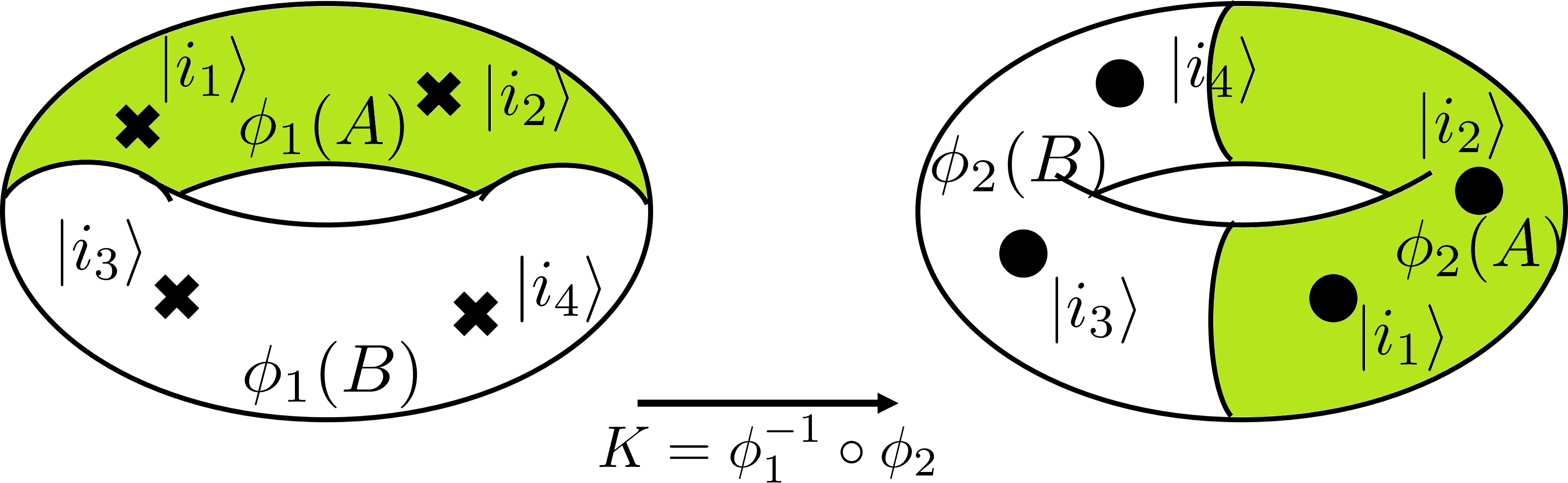
Figure 2: Same bipartition on sites can gives different bipartitions on space

In the case of TQFTs, the Hilbert space of functionals is reduced to a finite-dimensional Hilbert space of anyons if the gauge group and the manifold are compact TQFT1 ; TQFT2 . The coordinate transformations are also replaced by the mapping class group, which consists of topologically equivalent classes of transformations.

3 Partition functions, replica trick, and the surgery method

Here, we briefly introduce the method of computing TEE in the context of TQFT following TEEinCS . Consider the Chern-Simon action on a three manifold $M$

$$S_{\mathrm{CS}}=\frac{k}{4\pi}\int_{M}\mathrm{Tr}(A\wedge dA+A\wedge A\wedge A),$$ (3.1)

where $A$ is the connection one-form of the principal bundle of the underlying gauge group, and $k$ is the level of the theory. Doing a path integral over $M$ will give rise to a state in the Hilbert space of its boundary,

$$\ket{M}=\int\mathcal{D}A\,e^{-iS_{\mathrm{CS}}}\in\mathcal{H}_{\partial M}.$$ (3.2)

In general, one can also insert Wilson loops into the bulk to obtain different boundary states

$$\ket{M,C_{a}}=\int\mathcal{D}A\,e^{-iS_{\mathrm{CS}}[A]}W_{a}^{C}[A],$$ (3.3)

where the Wilson loop operator

$$W_{a}^{C}[A]=\mathrm{Tr}_{a}\mathcal{P}\{e^{\oint_{C}A}\}$$ (3.4)

traces the holonomy on a closed curve $C$ in representation $a$.

In particular, $\mathcal{H}_{T^{2}}$ is spanned by $\ket{a}=\ket{D^{2}\times S^{1},C_{a}}$, with $a$ ranging over the highest weight representations of the gauge group at level $k$ Ver ; TQFT1 ; TQFT2 . One can also construct the dual vectors by reversing the orientation of the manifold

$$\bra{a}=|\overline{D^{2}\times S^{1}},\overline{C_{a}}\rangle\in\mathcal{H}^{*}_{T^{2}}=\mathcal{H}_{\overline{T^{2}}}.$$ (3.5)

Partition function on $S^{2}\times S^{1}$ can be obtained by gluing two $D^{2}\times S^{1}$ with opposite orientation by identity map

$$Z(S^{2}\times S^{1},C_{\bar{a}},C_{b})=\bra{a}\ket{b}=\delta_{ab}.$$ (3.6)

On the other hand, one can also obtain the partition function of $S^{3}$ by gluing two $D^{2}\times S^{1}$ with opposite orientation related by the modular $S$ transformation

$$Z(S^{3},L_{ab})=\bra{a}S\ket{b}=S_{ab},$$ (3.7)

where $L_{ab}$ is the configuration of $C_{\bar{a}}$ and $C_{b}$ being linked once . In particular, if $a=b=0$, we obtain $Z(S^{2}\times S^{1})=1$ and $Z(S^{3})=S_{00}=D^{-1}$. Throughout this paper, we will refer to $\{\ket{a}\}_{a}$ as the inside basis and $\{S\ket{a}\}_{a}$ as the outside basis. We then have the basis transformation

$$S\ket{a}=\sum_{b}S_{ab}\ket{b}$$ (3.8)

Given a state $\ket{M}$, one can obtain the corresponding density matrix $\rho$ by the disjoint union of $M$ with $\overline{M}$. Given a bipartition $\partial M=A\cup B$, one can obtain the reduced density matrix $\rho_{A}=\mathrm{Tr}_{B}\rho$ by gluing $B$ of $M$ to the corresponding $B^{\prime}$ of $\overline{M}$ by the identity map. $\rho_{A}$ is then a manifold with boundary $A\cup A^{\prime}$, where $A^{\prime}$ is the corresponding region to $A$ in $\overline{M}$. One can then obtain $\mathrm{Tr}\rho_{A}^{2}$ by making two copies of $\rho_{A}$ and then perform two gluings from $A$ to $A^{\prime}$, which is a manifold without boundary. Similarly, $\mathrm{Tr}\rho_{A}^{n}$ can be constructed by $n$ copies of $M$ with corresponding gluings of the boundaries. One can then obtain the Rényi entropies

$$S_{n}=\frac{1}{1-n}\ln\mathrm{Tr}(\rho_{A})^{n}.$$ (3.9)

The entanglement entropy is then the limit $n\rightarrow 1$ by performing analytical continuation

$$S_{\mathrm{TEE}}=\lim_{n\rightarrow 1}S_{n}.$$ (3.10)

To evaluate the partition function of the glued manifold, one then applies the method of surgeryTQFT1 to decompose the manifold into simple ones whose partition functions are known, for example, Eq. (3.6) and Eq. (3.7).

Suppose one has a manifold $M$ without a boundary, which can be obtained by gluing $\overline{M_{1}},M_{2}$ along their common $S^{2}$ boundary

$$Z(M)=\bra{M_{1}}\ket{M_{2}}.$$ (3.11)

Due to the one dimensional property of $\mathcal{H}_{S^{2}}$, one has

$$\leavevmode\hbox{$\vbox{\hbox{\resizebox{}{}{{\leavevmode\hbox{\set@color{\includegraphics[height=128.0374pt]{surgery_1.png}}}}}}}$}\hskip 2.84544pt=\hskip 8.5359pt\leavevmode\hbox{$\vbox{\hbox{\resizebox{}{}{{\leavevmode\hbox{\set@color{\includegraphics[height=128.0374pt]{surgery_2.png}}}}}}}$}\hskip 2.84544pt.$$ (3.12)

Let $\tilde{M_{1}},\tilde{M_{2}}$ be the manifolds obtained by capping off the $S^{2}$ boundary with $D^{3}$ of $M_{1},M_{2}$ respectively, then

$$Z(M)Z(S^{3})=Z(\tilde{M_{1}})Z(\tilde{M_{2}}).$$ (3.13)

For example

  (3.14)

In general, one can also perform surgery with a Wilson loop insert due to the one dimensional property of $\mathcal{H}_{S^{2},a,\bar{a}}$ TQFT1 ; negativity

$$\leavevmode\hbox{$\vbox{\hbox{\resizebox{}{}{{\leavevmode\hbox{\set@color{\includegraphics[height=142.26378pt]{surgery_line_1.png}}}}}}}$}\hskip 2.84544pt=\hskip 8.5359pt\leavevmode\hbox{$\vbox{\hbox{\resizebox{}{}{{\leavevmode\hbox{\set@color{\includegraphics[height=142.26378pt]{surgery_line_2.png}}}}}}}$}\hskip 2.84544pt.$$ (3.15)

4 Topological entanglement entropy with different bipartitions, and the applications of the coordinate transformation

In this section, we apply the invariant property discussed in Sec. 2 to compute entropies using different coordinates. In Sec. 4.1, we will discuss bipartitions with a single $S^{1}$ interface as a consistency check of the method. In Sec. 4.2, we will discuss bipartitions with two $S^{1}$ interfaces being the meridians or the longitudes and obtain Verlinde-like formulas. In Sec. 4.3, we will discuss the case where the two $S^{1}$ interfaces are generic torus knots, which is made possible to compute by means of coordinate transformations.

4.1 Single $S^{1}$ interface

Consider the vacuum state $\ket{0}$ on $T^{2}$ generated by the empty solid doughnut $D^{2}\times S^{1}$ with a bipartition which has a single $S^{1}$ interface

$$\ket{0}=\hskip 5.69046pt\leavevmode\hbox{$\vbox{\hbox{\resizebox{}{}{{\leavevmode\hbox{\set@color{\includegraphics[height=68.28644pt]{donut_AB.png}}}}}}}$}\hskip 2.84544pt.$$ (4.1)

We consider the reduced density matrix

$$\rho_{A}=\mathrm{Tr}_{B}\rho=\mathrm{Tr}_{B}\outerproduct{0}{0}=\hskip 5.69046pt\leavevmode\hbox{$\vbox{\hbox{\resizebox{}{}{{\leavevmode\hbox{\set@color{\includegraphics[height=71.13188pt]{rho_A.png}}}}}}}$}\hskip 2.84544pt.$$ (4.2)

We can compute the $n$-th Rényi entropy by making $n$ copies of $\rho_{A}$ and gluing them together according to the boundary orientation. In the end, we will obtain that $\mathrm{Tr}{(\rho_{A}}^{n})$ is given by the connected sum of $n$ copies of $S^{2}\times S^{1}$.

$$\mathrm{Tr}{(\rho_{A}}^{n})=\hskip 2.84544pt\leavevmode\hbox{$\vbox{\hbox{\resizebox{}{}{{\leavevmode\hbox{\set@color{\includegraphics[height=56.9055pt]{n_torus.png}}}}}}}$}.$$ (4.3)

The partition function of such a configuration can be computed by the method of surgery similar to Eq. (3.14). By inserting $(n-1)$ copies of $S^{3}$ the configuration can be separated into $n$ copies of $S^{2}\times S^{1}$. The result is given by

$$\mathrm{Tr}{(\rho_{A}}^{n})=\frac{Z(S^{2}\times S^{1})^{n}}{Z(S^{3})^{n-1}}=D^{n-1}.$$ (4.4)

On the other hand, we can perform the same calculation using the outside basis instead. We know from Eq. (3.8) that the inside torus is related to the outside torus by the transformation

$$\leavevmode\hbox{$\vbox{\hbox{\resizebox{}{}{{\leavevmode\hbox{\set@color{\includegraphics[height=71.13188pt]{donut_AB_a.png}}}}}}}$}\hskip 2.84544pt=\sum_{b}S_{ab}\hskip 5.69046pt\leavevmode\hbox{$\vbox{\hbox{\resizebox{}{}{{\leavevmode\hbox{\set@color{\includegraphics[height=113.81102pt]{donut_AB_out.png}}}}}}}$}\hskip 2.84544pt,$$ (4.5)

where we use vertical torus to indicate the outside basis and the $S_{ab}$ is the modular $S$ matrix. Using the outside basis, the reduced density matrix is given by

$$\rho_{A}=\sum_{a,b}S_{0a}S_{0\bar{b}}\hskip 5.69046pt\leavevmode\hbox{$\vbox{\hbox{\resizebox{}{}{{\leavevmode\hbox{\set@color{\includegraphics[height=170.71652pt]{rho_A_out.png}}}}}}}$}\hskip 2.84544pt=\sum_{a,b}\frac{d_{a}}{D}\frac{d_{b}}{D}\hskip 8.5359pt\leavevmode\hbox{$\vbox{\hbox{\resizebox{}{}{{\leavevmode\hbox{\set@color{\includegraphics[height=142.26378pt]{rho_A_out_simp.png}}}}}}}$}\hskip 2.84544pt,$$ (4.6)

where $d_{a}=d_{\bar{a}}=S_{0a}D$ is the quantum dimension of anyon $a$ and $D=\sqrt{\sum_{a}d_{a}^{2}}$ is the total quantum dimension. For simplicity, we use a single black line to indicate a copy of $D^{2}\times S^{1}$, we use the dot to indicate that they are being connected summed and we use blue lines to indicate the anyon loops circling the corresponding non-contractible loops of $D^{2}\times S^{1}$. Using this notation, we have

$$\mathrm{Tr}{(\rho_{A}}^{n})=\sum_{a_{1},b_{1}}\sum_{a_{2},b_{2}}\dots\sum_{a_{n},b_{n}}\Big{(}\prod_{k=1}^{n}\frac{d_{a_{k}}d_{b_{k}}}{D^{2}}\Big{)}\hskip 5.69046pt\leavevmode\hbox{$\vbox{\hbox{\resizebox{}{}{{\leavevmode\hbox{\set@color{\includegraphics[height=142.26378pt]{Tr_rho_n.png}}}}}}}$}\hskip 2.84544pt,$$ (4.7)

where the double lines indicates that the two copies of $D^{2}\times S^{1}$ are glued together along their torus boundary to form a $S^{2}\times S^{1}$, and the giant dot indicates that these $S^{2}\times S^{1}$ are connected summed together. We should also mentioned that all the lines are all in the outside basis even if we do not put them in the vertical manner. To evaluate the partition function, we apply the method of surgery again to cut out all the separate $S^{2}\times S^{1}$’s with Wilson lines by inserting $S^{3}$’s. We then obtain

$$\mathrm{Tr}{(\rho_{A}}^{n})=\sum_{a_{1},b_{1}}\sum_{a_{2},b_{2}}\dots\sum_{a_{n},b_{n}}\prod_{k=1}^{n}\frac{d_{a_{k}}d_{b_{k}}}{D^{2}}\hskip 2.84544pt\leavevmode\hbox{$\vbox{\hbox{\resizebox{}{}{{\leavevmode\hbox{\set@color{\includegraphics[height=71.13188pt]{leg_a.png}}}}}}}$}\hskip 2.84544pt\leavevmode\hbox{$\vbox{\hbox{\resizebox{}{}{{\leavevmode\hbox{\set@color{\includegraphics[height=71.13188pt]{leg_b.png}}}}}}}$}\hskip 2.84544pt\frac{1}{Z(S^{3})^{n-1}}$$ (4.8)

Since the partition function of each $S^{2}\times S^{1}$ with Wilson lines $\bar{a},b$ is given by $\delta_{ab}$, and the partition function of $S^{3}$ is simply $D^{-1}$, we then have

$$\mathrm{Tr}{(\rho_{A}}^{n})=\Big{(}\sum_{a}\frac{d_{a}^{2}}{D^{2}}\Big{)}^{n}D^{n-1}=D^{n-1}.$$ (4.9)

As expected, we obtain the same result as using the inside basis. This serves as a consistency check of our method.

4.2 Two $S^{1}$ interfaces related by modular $S$ transformation

Next, we consider the case where the two sub-regions meet at two $S^{1}$ interfaces. If both $S^{1}$ interfaces are contractible, then the result will be similar to the case of a single interface. If only one $S^{1}$ is contractible, then the bipartition is ill-defined. The next possible bipartition is when the two interfaces are given by the same torus knots. In this subsection, we will consider the case where the torus knots are simply given by the longitudes and meridians.

4.2.1 Two $S^{1}$ interfaces being the longitudes of the torus

Consider the vacuum state in the solid torus and with the bipartition given by two longitudes which can be viewed as cutting the doughnut horizontally

$$\ket{0}=\hskip 5.69046pt\leavevmode\hbox{$\vbox{\hbox{\resizebox{}{}{{\leavevmode\hbox{\set@color{\includegraphics[height=85.35826pt]{donut_AB_3.png}}}}}}}$}\hskip 2.84544pt.$$ (4.10)

In this case, the reduced density matrix after tracing out $B$ is given by

$$\rho_{A}=\hskip 5.69046pt\leavevmode\hbox{$\vbox{\hbox{\resizebox{}{}{{\leavevmode\hbox{\set@color{\includegraphics[height=85.35826pt]{rho_A_3.png}}}}}}}$}\hskip 2.84544pt.$$ (4.11)

We have

$$\mathrm{Tr}({\rho_{A}}^{n})=Z(S^{2}\times S^{1})=1.$$ (4.12)

On the other hand, the calculation in the outside basis is rather non-trivial. Now we have

$$\ket{0}=\hskip 5.69046pt\leavevmode\hbox{$\vbox{\hbox{\resizebox{}{}{{\leavevmode\hbox{\set@color{\includegraphics[height=85.35826pt]{donut_AB_3.png}}}}}}}$}\hskip 2.84544pt=\sum_{a}S_{0a}\hskip 5.69046pt\leavevmode\hbox{$\vbox{\hbox{\resizebox{}{}{{\leavevmode\hbox{\set@color{\includegraphics[height=142.26378pt]{donut_AB_out_3.png}}}}}}}$}\hskip 2.84544pt,$$ (4.13)

where the bipartition also transforms with respect to the rewiring of sites as discussed in Sec. 2. We obtain the reduced density matrix $\rho_{A}$ by gluing $B$ to $B^{\prime}$,

$$\rho_{A}=\sum_{a,b}S_{0a}S_{0\bar{b}}\hskip 5.69046pt\leavevmode\hbox{$\vbox{\hbox{\resizebox{}{}{{\leavevmode\hbox{\set@color{\includegraphics[height=113.81102pt]{rho_A_out_3.png}}}}}}}$}=\sum_{a,b}S_{0a}S_{0b}\hskip 5.69046pt\leavevmode\hbox{$\vbox{\hbox{\resizebox{}{}{{\leavevmode\hbox{\set@color{\includegraphics[height=85.35826pt]{rho_A_out_3_simp.png}}}}}}}$}\hskip 2.84544pt.$$ (4.14)

Here the first graph in the left-hand side of Eq. (4.14), we flatten our solid torus to be an annulus for simplicity. The glued region indicated by color gray is $S^{2}\times D^{1}$ with two copies of $S^{2}$ boundaries. Also, each half solid torus ($A$ and $A^{\prime}$) has boundary being two copies of $D^{2}$. Therefore, two $D^{2}$ of separate $A$ and $A^{\prime}$ then be glued to form $S^{2}$ which matches each side of the boundary of the $S^{2}\times D^{1}$. The right-hand side of Eq. (4.14) is the view at the angle parallel to the radial direction of the circles (side view). For example,

$$\mathrm{Tr}{\rho_{A}}^{2}=\hskip 2.84544pt\leavevmode\hbox{$\vbox{\hbox{\resizebox{}{}{{\leavevmode\hbox{\set@color{\includegraphics[height=142.26378pt]{Tr_rho_2.png}}}}}}}$}\hskip 2.84544pt=\hskip 2.84544pt\leavevmode\hbox{$\vbox{\hbox{\resizebox{}{}{{\leavevmode\hbox{\set@color{\includegraphics[height=85.35826pt]{Tr_rho_2_string.png}}}}}}}$}\hskip 2.84544pt$$ (4.15)

With this notation, we have

$$\mathrm{Tr}{(\rho_{A}}^{n})=\sum_{\begin{subarray}{c}a_{1},\dots,a_{n}\\ b_{1},\dots,b_{n}\end{subarray}}\big{(}\prod_{i=1}^{n}\frac{d_{a_{i}}}{D}\frac{d_{b_{i}}}{D}\big{)}\hskip 2.84544pt.\leavevmode\hbox{$\vbox{\hbox{\resizebox{}{}{{\leavevmode\hbox{\set@color{\includegraphics[height=142.26378pt]{Tr_rho_n_3.png}}}}}}}$}\hskip 2.84544pt$$ (4.16)

We should note that each double line now represent $S^{2}\times D^{1}$ which is different from we have seen in Eq. (4.7). Each $S^{2}\times D^{1}$ has two disconnected $S^{2}$ boundaries and each $S^{2}$ boundary is separately connected summed to other corresponding $S^{2}$ boundaries. Next, we flatten the configuration by pushing all the handles ($S^{2}\times D^{1}$) in to the same plane in the following fashion

$$\leavevmode\hbox{$\vbox{\hbox{\resizebox{}{}{{\leavevmode\hbox{\set@color{\includegraphics[height=51.21504pt]{flatten.png}}}}}}}$}\hskip 2.84544pt=\hskip 2.84544pt\leavevmode\hbox{$\vbox{\hbox{\resizebox{}{}{{\leavevmode\hbox{\set@color{\includegraphics[height=56.9055pt]{flatten_2.png}}}}}}}$}\hskip 2.84544pt.$$ (4.17)

The right-land side of Eq. (4.17) is a connected sum of $S^{2}\times S^{1}$, where each hole represent a copy of $S^{2}\times S^{1}$. The anyon lines are given from left to right in the order $b_{1},a_{2},...,b_{k-1},a_{k},...b_{n-1},a_{n},b_{n}$ running in the same direction and $a_{1}$ winds all the holes. For example, one can refer to the left-hand side of Eq. (4.15) and deform it to the right-land side of Eq. (4.17) with three holes. We then apply the method of surgery by inserting $2n-2$ copies of $S^{3}$ with $a_{1}$ anyon loop as in Eq. (3.15). Therefore, we can obtain that

$$\mathrm{Tr}{(\rho_{A}}^{n})=\sum_{\begin{subarray}{c}a_{1},\dots,a_{n}\\ b_{1},\dots,b_{n}\end{subarray}}\prod_{i=1}^{n}\frac{d_{a_{i}}}{D}\frac{d_{b_{i}}}{D}\delta_{\bar{a_{1}}a_{i}}\delta_{\bar{a_{1}}b_{i}}\Big{(}\frac{D}{d_{a_{1}}}\Big{)}^{2n-2}=\sum_{a_{1}}\frac{d_{a_{1}}^{2}}{D^{2}}=1$$ (4.18)

Although the intermediate steps are less trivial, the final results using the outside basis and inside basis match.

4.2.2 Two $S^{1}$ interfaces being the meridians of the torus

Next, let us consider the vacuum state whose bipartition contain two meridians of the torus

$$\ket{0}=\hskip 5.69046pt\leavevmode\hbox{$\vbox{\hbox{\resizebox{}{}{{\leavevmode\hbox{\set@color{\includegraphics[height=71.13188pt]{donut_AB_2.png}}}}}}}$}\hskip 2.84544pt.$$ (4.19)

In this case, we have the reduced density matrix

$$\rho_{A}=\hskip 5.69046pt\leavevmode\hbox{$\vbox{\hbox{\resizebox{}{}{{\leavevmode\hbox{\set@color{\includegraphics[height=113.81102pt]{rho_A_2.png}}}}}}}$}\hskip 2.84544pt,$$ (4.20)

where we flatten the tori similar to previous section. Following the same procedure, we then obtain the same configuration as equation Eq. (4.17) but without the anyon lines. The final result is then a connected sum of $2n-1$ copies of $S^{2}\times S^{1}$. Therefore, we apply the method of surgery by inserting $2n-2$ copies of $S^{3}$ and get

$$\mathrm{Tr}{(\rho_{A}}^{n})=\frac{Z(S^{2}\times S^{1})^{2n-1}}{Z(S^{3})^{2n-2}}=D^{2n-2}.$$ (4.21)

Now, we do the same calculation but using the outside basis instead. The change of basis is

$$\ket{0}=\hskip 5.69046pt\leavevmode\hbox{$\vbox{\hbox{\resizebox{}{}{{\leavevmode\hbox{\set@color{\includegraphics[height=71.13188pt]{donut_AB_2.png}}}}}}}$}\hskip 2.84544pt=\sum_{a}S_{0a}\hskip 5.69046pt\leavevmode\hbox{$\vbox{\hbox{\resizebox{}{}{{\leavevmode\hbox{\set@color{\includegraphics[height=142.26378pt]{donut_AB_out_2.png}}}}}}}$}\hskip 2.84544pt.$$ (4.22)

Now, we have

$$\rho_{A}=\sum_{a,b}S_{0a}S_{0b}\hskip 5.69046pt\leavevmode\hbox{$\vbox{\hbox{\resizebox{}{}{{\leavevmode\hbox{\set@color{\includegraphics[height=142.26378pt]{rho_A_out_2.png}}}}}}}$}\hskip 2.84544pt,$$ (4.23)

and

$$\mathrm{Tr}{(\rho_{A}}^{n})=\sum_{a_{1},b_{1}}\sum_{a_{2},b_{2}}\dots\sum_{a_{n},b_{n}}\prod_{k=1}^{n}\frac{d_{a_{k}}d_{b_{k}}}{D^{2}}\hskip 2.84544pt\leavevmode\hbox{$\vbox{\hbox{\resizebox{}{}{{\leavevmode\hbox{\set@color{\includegraphics[height=142.26378pt]{Tr_rho_n_2.png}}}}}}}$}\hskip 2.84544pt$$ (4.24)

The partition function of $S^{2}\times S^{1}$ with anyon lines $a_{k}$, $b_{k}$ in its non-contractible loop is given by $\mathrm{dim}V_{a_{1},b_{1},\dots a_{n},b_{n}}$. Equating this to Eq. (4.21), we then obtain

$$\sum_{a_{1},b_{1}}\sum_{a_{2},b_{2}}\dots\sum_{a_{n},b_{n}}d_{a_{1}}d_{b_{1}}\dots,d_{a_{n}}d_{b_{n}}\mathrm{dim}V_{a_{1},b_{1},\dots a_{n},b_{n}}=D^{4n-2}.$$ (4.25)

This formula tells us that if we sum over the product of quantum dimensions of all the possible arrangements of $2n$ anyons weighted by the dimensions of the fusion trees $\mathrm{dim}V_{a_{1},b_{1},\dots,a_{n},b_{n}}$, then we obtain the total quantum dimension $D^{4n-2}$. Eq. (4.25) reminds us of the Verlinde formula Ver ; genVer , which also relates the quantum dimensions to the modular data. For example, in the case where $n=1$, $\mathrm{dim}V_{a_{1},b_{1}}=\delta_{a_{1},b_{1}}$, and thus we have the definition of quantum dimension $\sum_{a}d_{a}^{2}=D^{2}$. Although not quite obvious, one can also derive Eq. (4.25) using the Verlinde formula, which we will discuss in appendix A.

4.3 General Torus knot bipartitions

Now that we have established the consistency of entropy calculation using different coordinates, we can now compute the entanglement for more complicated configurations. In particular, we will consider bipartitions with two $S^{1}$ interfaces, both being torus knots. We will refer to such bipartitions as torus knot bipartitions throughout this paper. To visualize a torus knot bipartition, one can imagine a single torus knot on a torus, as in Fig. 3, and widen the line to become a ribbon that defines the subregion.

A general torus knot can be written as $K(k_{a},k_{b})$, where $k_{a}$ and $k_{b}$ are integers with $\mathrm{gcd}(k_{a},k_{b})=1$. Let $K(1,0)$ and $K(0,1)$ denote the meridians and the longitudes, then $K(k_{a},k_{b})$ is a torus knot that winds $k_{a}$ and $k_{b}$ times in the meridian and longitude direction, respectively. For example, Fig. 3 shows a torus knot $K(8,3)$.

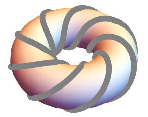
Figure 3: Torus knot $K(8,3)$ embedded in $\mathbb{R}^{3}$ and on its fundamental domain.

Suppose we have a bipartition $T^{2}=A\amalg B$, with interfaces $\partial A=\partial B$ composed of two copies of $S^{1}$, then the two $S^{1}$ should be the same torus knot to avoid intersecting with each other. Therefore, we can uniquely determine a torus knot bipartitions by the type of torus knots its interfaces are made of.

Let us consider a vacuum state with no Wilson lines inserted and a torus knot bipartition with the interface being the torus knot $K(k_{a},k_{b})$ with $\mathrm{gcd}(k_{a},k_{b})=1$. By applying modular $S$ and $T$ transformations, one can transform $K(k_{a},k_{b})$ into $K(k_{b},k_{a})$ and $K(k_{a},k_{b}+k_{a})$, respectively. Therefore, using the Euclidean algorithm, one can transform any torus knot into the meridian $K(1,0)$ by a series of modular $S$ and $T$ transformations.

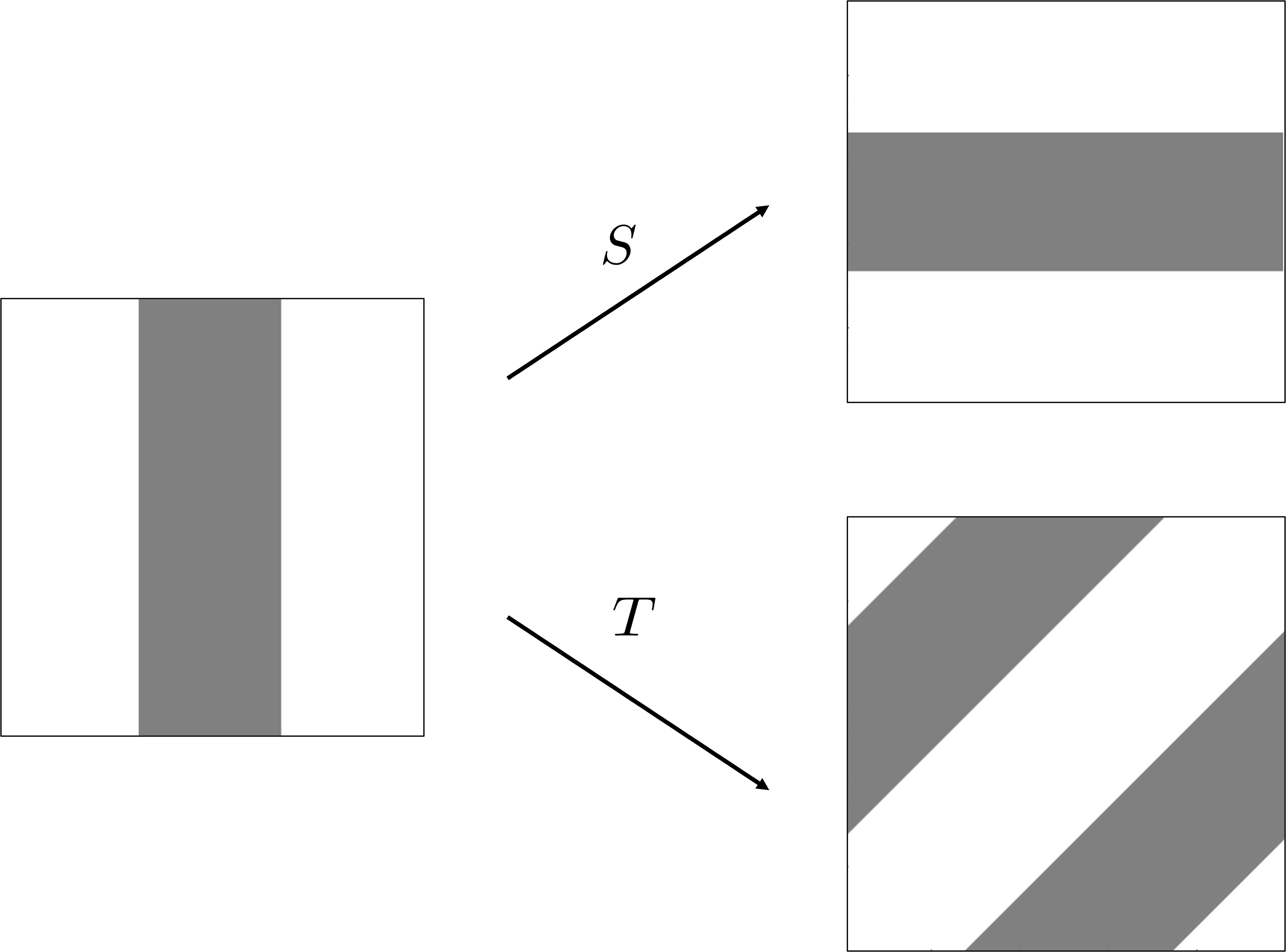
Figure 4: The modular $S$ and $T$ transformation generate the whole modular group $SL(2,\mathbb{Z})$.

That is, all the possible torus knot bipartitions can be mapped back to the canonical bipartition consist of meridian interfaces by some $\mathcal{O}\in SL(2,\mathbb{Z})$. For example, $K(8,3)$ can be turned into the canonical bipartition by the sequentially application of $ST^{2}S^{-1},T,ST^{2}S^{-1},S$ on the torus. The combined transformation is then given by $\mathcal{O}=SST^{2}S^{-1}TST^{2}S^{-1}=(ST)^{-1}$. With the expression of $\mathcal{O}$, we rewrite

$$\ket{0}=\mathcal{O}\mathcal{O}^{-1}\hskip 5.69046pt\leavevmode\hbox{$\vbox{\hbox{\resizebox{}{}{{\leavevmode\hbox{\set@color{\includegraphics[height=85.35826pt]{torus_eg_1}}}}}}}$}\hskip 2.84544pt=\sum_{a}\mathcal{O}_{0a}\hskip 5.69046pt\leavevmode\hbox{$\vbox{\hbox{\resizebox{}{}{{\leavevmode\hbox{\set@color{\includegraphics[height=85.35826pt]{donut_AB_2_a.png}}}}}}}$}\hskip 2.84544pt.$$ (4.26)

The gray line in the left figure of Eq. (4.26) indicate the subregion $A$ and the solid torus has no Wilson lines insert. In the right figure of Eq. (4.26), the coordinate grid is twisted compared to the left figure. However, we can perform exactly the same replica method in the new coordinate system as long as all the copies are in the same coordinate. Following similar calculation in the previous sections, we then obtain that

$$\mathrm{Tr}{(\rho_{A}}^{n})=\sum_{\begin{subarray}{c}a_{1},\dots,a_{n}\\ b_{1},\dots,b_{n}\end{subarray}}\prod_{i=1}^{n}\mathcal{O}_{0a_{i}}\mathcal{O}^{*}_{0b_{i}}\delta_{a_{1}a_{i}}\delta_{a_{1}b_{i}}\Big{(}\frac{D}{d_{a_{1}}}\Big{)}^{2n-2}=\sum_{a}\frac{|\mathcal{O}_{0a}|^{2n}}{(S_{0a})^{2n-2}}$$ (4.27)

Taking the limit $n\rightarrow 1$, we then obtain the topological entanglement entropy. One interesting observation is that if we define $\psi_{a}=\mathcal{O}_{0a}$, then the TEE is given by

$$S_{A}=\sum_{a}2|\psi_{a}|^{2}(\ln d_{a}-\ln|\psi_{a}|)-2\ln D.$$ (4.28)

This is exactly the same as computed in EdgeTEE for a generic ground state in the edge theory approach. That is, although we start with a vacuum state, the twisted bipartition induces an effective state which is no longer vacuum. In general, if we start with a state $\ket{\psi}=\sum_{a}\psi_{a}\ket{a}$ with a torus knot bipartition, which can be rotated back to the canonical bipartition by an operator $\mathcal{O}$, the effective state is then given by $\ket{\psi^{\prime}}=\sum_{a,b}\mathcal{O}_{ab}\psi_{b}\ket{a}$. For our $K(8,3)$ example where the initial state has no Wilson lines insert, the effective state is given by $\ket{\psi^{\prime}}=\sum_{a,b}(ST)^{-1}_{ab}\delta_{0b}\ket{a}=\sum_{a}T^{*}_{aa}S_{0a}\ket{a}$. The topological entanglement entropy is then given by

$$S_{A}=\sum_{a}2(S_{0a})^{2}(\ln d_{a}-\ln S_{0a})-2\ln D=0.$$ (4.29)

We have shown that the entropy for an arbitrary ground state and an arbitrary torus knot bipartition can be written as Eq. (1.1), where the ground state TEE is given by

$$S_{\mathrm{gs}}=\sum_{a}2|\psi_{a}|^{2}(\ln d_{a}-\ln|\psi_{a}|),$$ (4.30)

for a given state $\ket{\psi}=\sum_{a}\psi_{a}\ket{a}$ depending on the twists of bipartition. This ground state TEE is bounded by.

$$0\leq S_{\mathrm{gs}}\leq 2\ln D.$$ (4.31)

That is, in the context of TQFT, $-2\ln D$ shown in TEE ; TEE2 is the lower bound for the TEE of any bipartition independent of the anyon type, ground state, and the bipartition as long as the number of interfaces is fixed. The TEE correction due to the ground state and the Dehn twist of bipartition will always be non-negative.

5 Conclusion

In this paper, we apply the invariant property of the entanglement quantities under coordinate transformations for generic torus knots bipartitions. We demonstrate a Verlinde-like formula can be derived. We find the TEE of torus knots bipartitions with twists can be decomposed into a state independent part which depends only on the interface and a non-negative correction caused by effective Wilson lines inserted into the system. As a final remark, in the follow-up paper CYL , we will discuss a general decomposition of the TEE

$$S_{\mathrm{TEE}}(A,\psi)=S_{\mathrm{min}}(A)+S_{\mathrm{gs}}(A,\psi),$$ (5.1)

where

$$S_{\mathrm{min}}(A)=\min_{\ket{\psi}}S_{\mathrm{TEE}}(A,\ket{\psi})\leq 0,$$ (5.2)

is a universal topological quantity that depends only on the number of interfaces of the bipartition, and $S_{\mathrm{gs}}\geq 0$ is a quantity that detects effective ground states caused by the twisted bipartition or the Wilson loop inserted in the system. Overall, the value of this correction term will never exceed the absolute value of the universal term, ensuring that the total TEE, i.e., $S_{\mathrm{TEE}}$ is always non-positive. Furthermore, we can also show that $S_{\mathrm{gs}}$ behaves just like the usual entanglement entropy, as it is non-negative and satisfies both the strong subadditivity and the subadditivity. $S_{\mathrm{TEE}}$, on the other hand, is always non-positive and only satisfies the strong subadditivity.

6 Acknowledgments

We are grateful to Xueda Wen for useful discussions. P.-Y.C. acknowledges support from the National Science and Technology Council of Taiwan under Grants No. NSTC 112-2636-M-007-007 and No. 112-2112-M-007-043. Both P.-Y.C and C.-Y. L. thank the National Center for Theoretical Sciences, Physics Division for their support.

Appendix A The Verlinde-like formula

Here, we derive Eq. (4.25) by using the Verlinde formula. The Verlinde formula states that the fusion rules can be simultaneously diagonalized by the modular $S$ matrices Ver

$$\mathrm{dim}V^{a}_{bc}=(N_{c})^{a}_{b}=(N_{b})^{a}_{c}=\sum_{d}\frac{S_{bd}S_{cd}S^{*}_{da}}{S_{0d}}.$$ (A.1)

One can generalize this to $n$ anyons by factorizing the fusion trees

$$V^{0}_{a_{1},\dots a_{n}}=\sum_{c_{2},\dots c_{n-1}}\prod_{i=2}^{n}V^{c_{i}}_{c_{i-1}a_{i}},$$ (A.2)

where $c_{n-1}=0$ and $c_{1}=a_{1}$. Substituting the Verlinde formula into the above expression, we then obtain

$$\mathrm{dim}V^{0}_{a_{1},\dots a_{n}}=\sum_{\begin{subarray}{c}c_{2},\dots,c_{n-1}\\ d_{2},\dots,d_{n}\end{subarray}}\prod_{i=2}^{n}\frac{S_{a_{i}d_{i}}S_{c_{i-1}d_{i}}S^{*}_{d_{i}c_{i}}}{S_{0d_{i}}}.$$ (A.3)

Sum over the internal $c_{i}$’s for $i=2,\dots,n-1$ with $\sum_{c_{i}}S^{*}_{d_{i}c_{i}}S_{c_{i}d_{i+1}}=\delta_{d_{i}d_{i+1}}$, one has

$$\mathrm{dim}V^{0}_{a_{1},\dots a_{n}} =\sum_{d_{2},\dots,d_{n}}S_{c_{1}d_{2}}\Big{(}\prod_{i=2}^{n-1}\frac{S_{a_{i}d_{i}}\delta_{d_{i}d_{i+1}}}{S_{0d_{i}}}\Big{)}\frac{S_{a_{n}d_{n}}S^{*}_{c_{n-1}d_{n}}}{S_{0d_{n}}}$$ (A.4)

$$=\sum_{d}\Big{(}\prod_{i=1}^{n}\frac{S_{a_{i}d}}{S_{0d}}\Big{)}(S_{0d})^{2}.$$

This is the Verlinde-like formula discussed in genVer . Now, substituting in $S_{0a}=S^{*}_{0a}=d_{a}$, $S_{00}^{-1}=D$ and $S^{2}=C$, the charge conjugation operator, one arrive at

$$\sum_{a_{1},\dots,a_{n}}\big{(}\prod_{i=1}^{n}d_{a_{i}}\big{)}\mathrm{dim}V^{0}_{a_{1},\dots a_{n}}=\sum_{d}\Big{(}\prod_{i=1}^{n}\frac{C_{0d}}{S_{00}S_{0d}}\Big{)}(S_{0d})^{2}=D^{2n-2}.$$ (A.5)

This is exactly equation Eq. (4.25) by setting $n$ to $2n$ due to the presence of both $a_{k}$ and $b_{k}$.

Appendix B The bounds on ground state TEE

Here, we give a brief proof of Eq. (4.31). Since we are extremizing under the constraint $\sum_{a}|\psi_{a}|^{2}=1$, we can employ the method of Lagrange multiplier by defining

$$\tilde{S}_{\mathrm{gs}}=\sum_{a}2|\psi_{a}|^{2}(\ln d_{a}-\ln|\psi_{a}|)-\lambda(\sum_{a}|\psi_{a}|^{2}-1).$$ (B.1)

Differentiating with respect to $|\psi_{a}|$ yields

$$2(\ln d_{a}-\ln|\psi_{a}|)-1=2\lambda,$$ (B.2)

which normalizes to $|\psi_{a}|=S_{0a}$. That is, the extremum of $S_{\mathrm{gs}}$ happens only if $|\psi_{a}|=S_{0a}$ or $|\psi_{a}|$ takes boundary values . Therefore, one then verify that $S_{\mathrm{gs}}$ takes minimum $S_{\mathrm{gs}}=0$ when $|\psi_{a}|=\delta_{a0}$ and takes maximum $S_{\mathrm{gs}}=2\ln D$ when $|\psi_{a}|=S_{0a}$ for all $a$.

References

- (1) E. Witten, Quantum Field Theory and the Jones Polynomial, Commun.Math.Phys. 121 (1989) .
- (2) S. Elitzur, G. Moore, A. Schwimmer and N. Seiberg, Remarks on the canonical quantization of the Chern-Simons-Witten theory, Nucl.Phys.B 326 (1989) .
- (3) D. Tsui, H. Stormer and A. Gossard, Two-dimensional magnetotransport in the extreme quantum limit, Phys. Rev. Lett. 48 (1982) .
- (4) R. Laughlin, Anomalous Quantum Hall Effect: An Incompressible Quantum Fluid with Fractionally Charged Excitations, Phys. Rev. Lett. 50 (1983) .
- (5) X.-G. Wen, Topological orders and Edge excitations in FQH states, Advances in Physics 44 (1995) .
- (6) H. Li and F. D. M. Haldane, Entanglement Spectrum as a Generalization of Entanglement Entropy: Identification of Topological Order in Non-Abelian Fractional Quantum Hall Effect States, Phys. Rev. Lett. 101 (2008) .
- (7) X.-G. Wen, Quantum Orders and Symmetric Spin Liquids, Phys. Rev. B 65 (2002) .
- (8) D. S. Rokhsar and S. A. Kivelson, Superconductivity and the Quantum Hard-Core Dimer Gas, Phys. Rev. Lett. 61 (1988) .
- (9) M. Stone and S. B. Chung, Fusion rules and vortices in px+ipy superconductors, Phys. Rev. B 73 (2006) .
- (10) X. Weng, Topological Order in Rigid States, Int.J.Mod.Phys.B 4 (1990) .
- (11) A. Kitaev and J. Preskill, Topological entanglement entropy, Phys.Rev.Lett. 96 (2006) .
- (12) M. Levin and X.-G. Wen, Detecting topological order in a ground state wave function, Phys.Rev.Lett. 96 (2006) .
- (13) M. Srednicki, Entropy and Area, Phys.Rev.Lett. 71 (1993) .
- (14) M. Haque, O. Zozulya and K. Schoutens, Entanglement entropy in fermionic Laughlin states, Nature Physics 7 (2007) .
- (15) H.-C. Jiang, Z. Wang and L. Balents, Identifying Topological Order by Entanglement Entropy, Nature Physics 8 (2012) .
- (16) H. Li and F. D. M. Haldane, Entanglement Spectrum as a Generalization of Entanglement Entropy: Identification of Topological Order in Non-Abelian Fractional Quantum Hall Effect States, Phys. Rev. Lett. 101 (2008) .
- (17) H. Li and F. D. M. Haldane, Entanglement Spectrum as a Generalization of Entanglement Entropy: Identification of Topological Order in Non-Abelian Fractional Quantum Hall Effect States, Phys. Rev. Lett. 101 (2008) .
- (18) S. V. Isakov, M. B. Hastings and R. G. Melko, Topological Entanglement Entropy of a Bose-Hubbard Spin Liquid, Nature Physics 7 (2011) .
- (19) S. Dong, E. Fradkin, R. G. Leigh and S. Nowling, Topological Entanglement Entropy in Chern-Simons Theories and Quantum Hall Fluids, JHEP 016 (2008) .
- (20) X. Wen, P.-Y. Chang and S. Ryu, Topological entanglement negativity in Chern-Simons theories, JHEP 09 (2016) .
- (21) R. Sohal and S. Ryu, Entanglement in tripartitions of topological orders: a diagrammatic approach, Phys. Rev. B 108 (2023) .
- (22) X. Wen, S. Matsuura and S. Ryu, Edge theory approach to topological entanglement entropy, mutual information and entanglement negativity in Chern-Simons theories, Phys. Rev. B 93 (2016) .
- (23) T. Nishioka, T. Takayanagi and Y. Taki, Topological pseudo entropy, JHEP 09 (2021) .
- (24) P. Bonderson, C. Knapp and K. Patel, Anyonic Entanglement and Topological Entanglement Entropy, Annals of Physics 385 (2017) .
- (25) S. Dwivedi, V. K. Singh, P. Ramadevi, Y. Zhou and S. Dhara, Entanglement on multiple S2 boundaries in Chern-Simons theory, JHEP 08 (2019) .
- (26) J. R. Fliss, X. Wen, O. Parrikar, C.-T. Hsieh, T. L. H. Bo Han and R. G. Leigh, Interface Contributions to Topological Entanglement in Abelian Chern-Simons Theory, JHEP 09 (2017) .
- (27) Y. Zhang, T. Grover, A. Turner, M. Oshikawa and A. Vishwanath, Quasi-particle Statistics and Braiding from Ground State Entanglement, Phys. Rev. B 85 (2012) .
- (28) E. P. Verlinde, Fusion Rules and Modular Transformations in 2D Conformal Field Theory, Nucl.Phys.B 300 (1988) .
- (29) G. W. Moore and N. Seiberg, Classical and Quantum Conformal Field Theory, Commun.Math.Phys. 123 (1989) .
- (30) C.-Y. Lo and P.-Y. Chang, Strong subadditivity for topological entanglement entropy, in preparation .