Spectro-photometric properties of CoPhyLab’s dust mixtures

Abstract

Objective: In the framework of the Cometary Physics Laboratory (CoPhyLab) and its sublimation experiments of cometary surface analogues under simulated space conditions, we characterize the properties of intimate mixtures of juniper charcoal and SiO₂ chosen as a dust analogue (Lethuillier et al., 2022). We present the details of these investigations for the spectrophotometric properties of the samples.
Methods: We measured these properties using a hyperspectral imager and a radio-goniometer. From the samples’ spectra, we evaluated reflectance ratios and spectral slopes. From the measured phase curves, we inverted a photometric model for all samples. Complementary characterizations were obtained using a pycnometer, a scanning electron microscope and an organic elemental analyser.
Results: We report the first values for the apparent porosity, elemental composition, and VIS-NIR spectrophotometric properties for juniper charcoal, as well as for intimate mixtures of this charcoal with the SiO₂. We find that the juniper charcoal drives the spectro-photometric properties of the intimate mixtures and that its strong absorbance is consistent with its elemental composition. We find that SiO₂ particles form large and compact agglomerates in every mixture imaged with the electron microscope, and its spectrophotometric properties are affected by such features and their particle-size distribution. We compare our results to the current literature on comets and other small Solar System bodies and find that most of the characterized properties of the dust analogue are comparable to some extent with the spacecraft-visited cometary nucleii, as well as to Centaurs, Trojans and the bluest TNOs.

1 Introduction

Small bodies of the Solar System are tracers of the evolutionary processes that occurred since the earliest stages of its formation from the Solar nebula. Characterising not only these objects’ dynamical and bulk properties, but also their surface properties is an essential step to complete our understanding of their nature, and thus to refine our knowledge of the Solar System’s history. While an handful of sample return missions have granted a first-hand knowledge of the compositional and surface properties of a few small bodies, ground- and space-based remote sensing have provided the bulk of our understanding for asteroids, comets and other small bodies of the Solar System.

Comets, in particular, are virtually time-capsules, and the study of their physical properties as well as their composition, largely preserved since their formation more than 4.5 billions of years ago, has allowed to make direct inferences on the properties of the proto-planetary disk from which they accreted. (Davidsson et al., 2016; Rubin et al., 2019; Drozdovskaya et al., 2019). Over the last forty years, successive space missions have allowed us to observe and investigate comae and nuclei in ever greater details (e.g. Muench et al. 1986; A’ Hearn et al. 2011). To this day, the ESA-led Rosetta mission provided the most complete picture of a comet, as it accompanied 67P/Churyumov-Gerasimenko (hereafter 67P/C-G) throughout its 2015 perihelion passage. From August 2014 to September 2016, the Rosetta spacecraft provided a multi-instrument monitoring of the comet’s inner coma and its nucleus’ surface properties, and in November 2014, the Philae probe performed in-situ measurements as it landed on the nucleus (Taylor et al., 2017).
The chemical compounds directly identified in the inner coma and at the surface of 67P/C-G’s nucleus (Altwegg et al., 2019; Hänni et al., 2022; Bardyn et al., 2017; Krüger et al., 2017) complete our understanding of cometary composition derived, from instance, from the laboratory analysed dust particles of comet 81P/Wild-2’s coma (Brownlee et al., 2012; Sandford et al., 2021). The quantitative interpretation of remote-sensing data suffers however from the lack of ground-truth. While models exist that relate photometric observables to physico-chemical properties of the surfaces, some of the approximations are purely empirical and the complexity of natural surfaces often results in degeneracies when inverting the models. In this context, laboratory studies of the properties and behaviour of surface analogues under cometary conditions can help to provide a more thorough understanding and interpretation of remote-sensing measurements to better refine scenarios for the formation and evolution of comets.

The Cometary Physics Laboratory (CoPhyLab) project follows a multi-disciplinary approach to characterize both the evolution of the physical properties and the phenomena on and inside the surface of a cometary analogue under simulated space conditions, using multiple instruments (Kreuzig et al., 2021). One of the initial objectives of the CoPhyLab project consisted in the definition of a suitable and workable cometary analogue recipe as a compromise between the suitability of the chosen materials, their level of characterization as well as practical considerations such as ease of procurement, cost and relative harmlessness (Lethuillier et al., 2022). Of particular importance for many investigations planned in this project is the albedo of the final dust simulant as this property has a direct impact on the absorption of solar radiation and therefore on the thermo-physical processes that affect the material. Other photometric properties should ideally be as close as possible to actual known properties of cometary nuclei to ensure that the light scattering regimes are comparable. This facilitates the direct comparison between experimental results and remote-sensing datasets and the validation on laboratory samples of the physical models ultimately used to invert composition and physical properties from reflectance. Studying chemical processes was not an objective of the CoPhyLab project and therefore reproducing the known chemical composition of the nucleus was not a primary criterion in the analogue selection. As the composition of the analogue differs significantly and is much simpler than the one of actual cometary material, one cannot expect all spectro-photometric properties to match. It is nevertheless important to characterize their differences to interpret correctly the implications of laboratory results in the context of actual comets observations.

Past attempts at simulating cometary processes in the laboratory have made use of a variety of materials. During the KOSI experiments, olivine, kaoline and montomorillonite were intimately mixed with carbon to produce a dark cometary dust simulant, which was then mixed with ice. Oehler & Neukum (1991) note however that the addition of carbon in the mixture masks all absorption features by minerals, flattening the spectrum. Carbon and carbon-based compounds have been used in a number of other studies to achieve a low albedo (Stephens & Gustafson, 1991; Moroz et al., 1998a). More recently, opaque minerals have also been used for a similar purpose. (Quirico et al., 2016; Rousseau et al., 2017). In the framework of the CoPhyLab project, the search for a suitable dust analogue ultimately resulted in the selection of silicon dioxide and juniper charcoal as the two components for the first dust recipe of the CoPhyLab project. As a complement to the companion study of Lethuillier et al. 2022, the present work was performed to characterize the spectroscopic and photometric properties of the two materials chosen to simulate cometary surfaces, as well as to investigate the properties of intimate mixtures formed from these two materials. Mixed together in the right proportions, these two components display an albedo similar to the nucleus while other key physical and spectro-photometric properties are also reasonably close. The measurements of our study are a counterpart to those obtained, for instance, by the OSIRIS and VIRTIS instruments of the ROSETTA mission. Combined, such measurements allow to correlate the reflectance of a material with both its compositional and physical properties, e.g. through the identification of specific absorption bands, or the estimation of the albedos. Furthermore, such measurements will serve as references for future CoPhyLab sublimation experiments, and complement other physical measurements described in Kreuzig et al. 2021, to provide a more accurate modelling of the analogue material and the subsequent interpretation of both CoPhyLab and remote-sensing observations.

In section 2, we present the materials and the instruments used as well as the data reduction process before outlining the photometric model used in this study. In section 3, we present the results of the spectroscopic measurements and of the photometric modelling. Finally, we discuss our results in the light of the existing literature in section 4.

2 The materials, instruments and photometric model used

2.1 End-members of the CoPhyLab dust recipe

The silicon dioxide powder (SiO₂, CAS: 14808-60-7) was obtained from Honeywell (REF: S5631). Although the particle size distribution (PSD) ranges from 0.5 $\mu$m to 10 $\mu$m, as reported in Kothe et al. (2013), we observe that the SiO₂ particles easily form large aggregates with a diameter up to a few millimetres. Scanning electron microscope images (Fig 1, left column) illustrate that such large SiO₂ aggregates (top image) are formed by the apparent regular assemblage of grains a few hundreds of nanometres in size and micrometer-sized chunks (bottom image), sticking to and stacked upon each another.

As reported in Lethuillier et al. (2022), we performed porosity m easurements through two methods: using a 1 mL graduated flask to determine the powder’s bulk density, and using an helium pycnometer (Upyc-1200e-V5.04) to measure the apparent particle volume (i.e. the sum of the solid material volume and that of any closed void), thus allowing to retrieve the apparent particle density Svarovskly (1987).

Assuming homogeneous particles, we found the SiO₂ powder sample to have a bulk density of 0.885$\pm$0.001 g.cm^-3, and an apparent particle density of 2.59$\pm$0.02 g.cm^-3. The associated porosity for this sample thus stands at 65$\pm$3%. These values are consistent with prior measurements on a similar material using different methods Kothe et al. (2013).

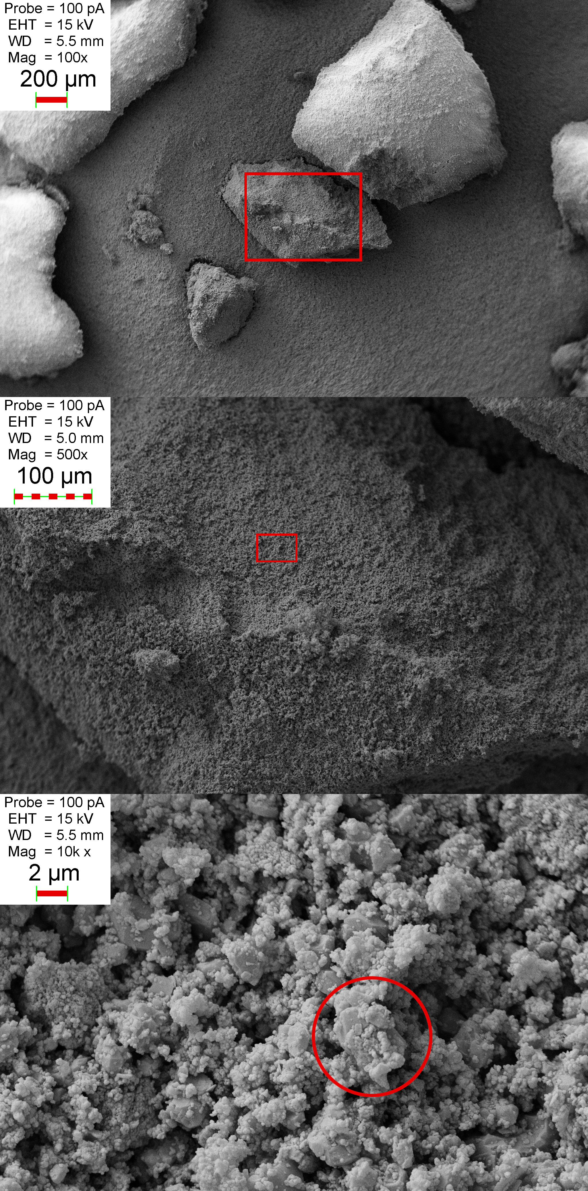
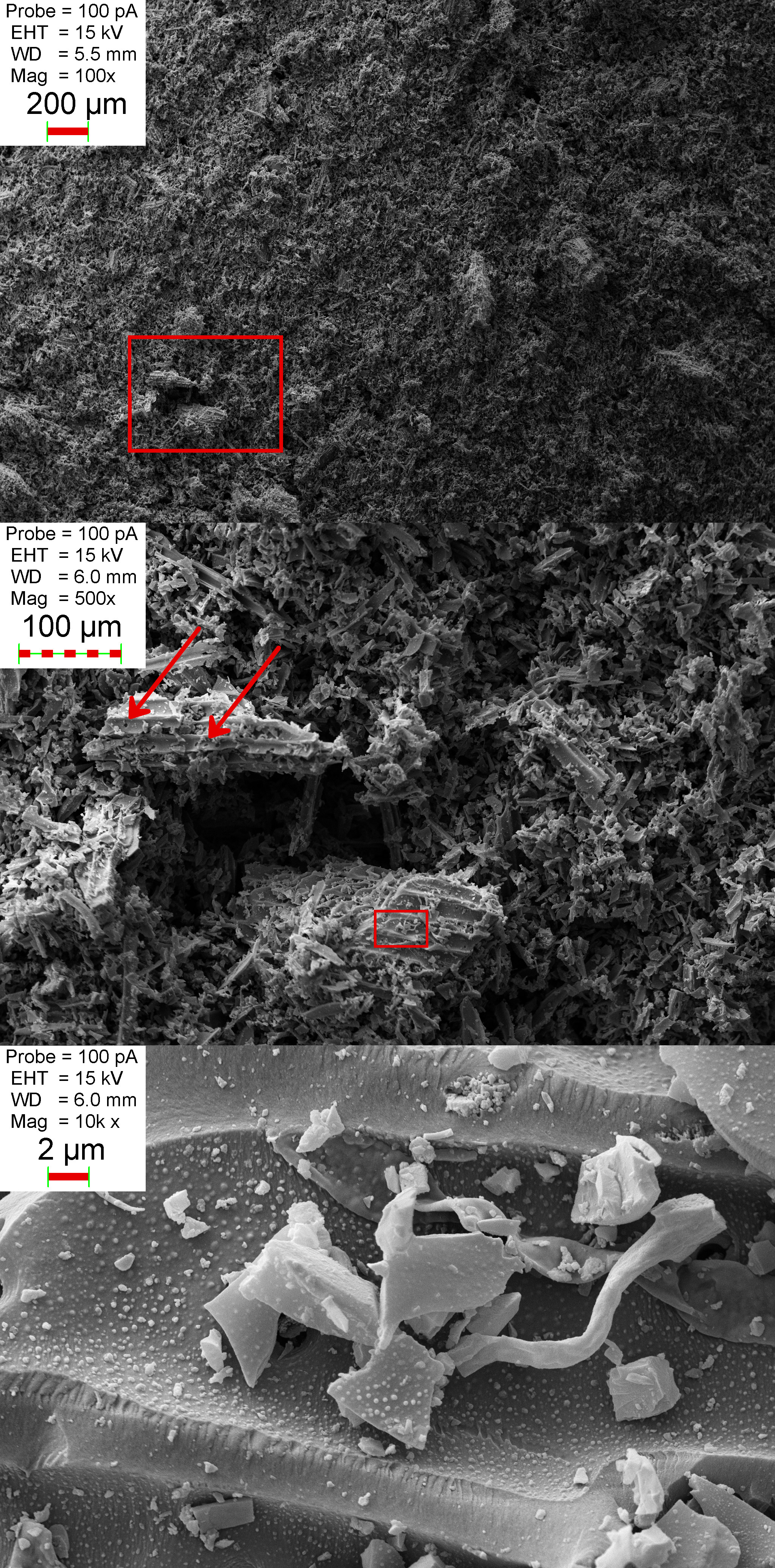
Figure 1: SiO₂ and JChc samples observed under a scanning electron microscope (SEM) at increasing magnification settings (from top to bottom). Left column: Zooming-in on millimetre-sized SiO₂ aggregates reveals nanometre-sized grains heaping on each other as well as upon larger particles, such as the one encircled in red in the bottom picture. – Right column: Zooming-in on the juniper charcoal sample exposes a tangle of micrometre- and nanometre-sized wood vessel structures and fragments, such as wall pores (red arrows, middle picture) and lignin protuberances (warty surfaces, bottom picture), which survived the carbonisation, grinding and sieving processes.

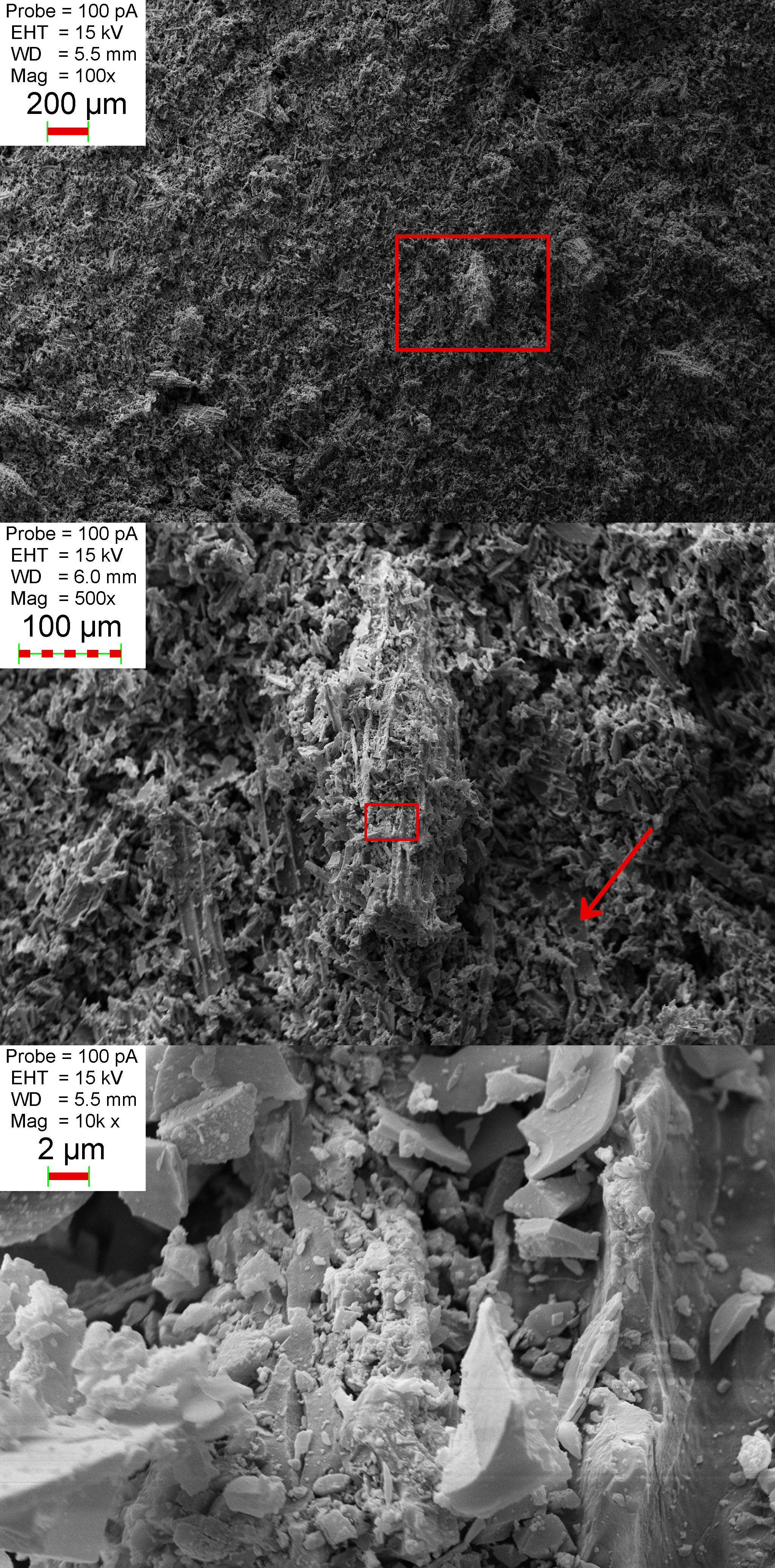
Figure 9: Alternate zoom on a remnant of the juniper wood structure illustrating the wide range of particle-sizes present in the juniper charcoal sample, which spawns from the tens of nanometers to the hundreds of micrometers. In the middle picture, the red arrow points to a pore in another juniper wood remnant of a vessel wall.

The juniper charcoal powder (hereafter, JChc) was obtained from the firm Werth-Metall. No specific information could be obtained on the manufacturing process, except that the powder had been sieved using a 100 $\mathrm{\mu}$m mesh sieve. As per the initial CoPhyLab dust recipe, the juniper charcoal sample was further dry-grounded using an agate disk mill (of the Retsch RS200 model), set at 700 rpm for about two and a half minute, and then the smallest particle-size fraction was extracted using a 50 $\mathrm{\mu}$m mesh sieve.
As for the SiO₂ sample, SEM images of the JChc sample are presented in Fig. 1, right column). Even at the lowest magnification setting (right column, top picture), the JChc sample appears to contain a number of elongated (“splinter”-like) particles with dimensions reaching $\sim$ 70 $\mathrm{\mu}$m emerging out, or laying on top, of an agglomerate of smaller particles. Such flat splinters can pass in the diagonal of the 50 $\mathrm{\mu}$m square mesh sieves. Some of these particles (center and bottom images of Fig. 1, right column, as well as Fig. 9) clearly display the structures of wood cells (e.g. Forest Products Laboratory 1980, Jiang et al. 2018), such as pores on vessel walls (pointed by the red arrows in Fig. 1), or lignin protuberances (the distinct wart-like surfaces in the bottom image of the same figure). While features such as pores are $\sim$ 2 $\mathrm{\mu}$m in diameter, lignin protuberances are a few hundreds of nanometre in size. As illustrated by the center and bottom images of Figs. 1 and 9, smaller JChc particles exhibit diversity in shapes: from sub-micrometre grains through micrometre-sized pieces and platelets to tens-of-micrometre-sized fragments of vessel walls.

Finally, the bulk and apparent particle densities of the JChc sample were found to be respectively equal to 0.479$\pm$0.001 g.cm^-3 and 1.5$\pm$0.1 g.cm^-3, thus giving a porosity of 68$\pm$3%. Although no literature references were found for this specific charcoal, these values are consistent with those obtained for different types of charcoal, such as beech charcoal (Brocksiepe, 2000).

2.2 Preparation of the mixtures

As presented in Lethuillier et al. (2022), a series of 9 intimate binary mixtures of SiO₂ and JChc were prepared with steps of 10 wt.% in the JChc mass fraction. The first mixture thus contained 10% JChc by mass, and the last one 90%.
In order to produce these mixtures, we proceeded systematically in this way: the whole of the minor fraction was first placed in a bottle in which the major fraction was then progressively introduced. With each addition of the major fraction material, the bottle was gently shaken by hand for 10 seconds to homogenize the mixture. Any agglomerate larger than a few millimetres, that formed during the shaking, was broken apart with a spatula. We decided to use a manual shaking as initial tests with a mechanical shaker immediately produced a number of such large agglomerates.
Using this procedure, $\sim$ 12 g of each mixture were prepared, an amount sufficient to fill either type of sample holder used in the radio-goniometric and spectroscopic measurements.

For either type of measurements, all of the samples were prepared in a similar manner. Black-anodized aluminium containers were filled up to rim using a spatula and a final layer of material was sprinkled using a large sieve (1.5mm mesh size) to obtain a random surface orientation and avoid material compression.
The pictures of the samples prepared in this way are presented in Fig. 13.

2.3 Spectroscopic measurements

Using the Mobile Hyperspectral Imaging Setup (MoHIS) of the University of Bern, hyperspectral VIS-NIR cubes with a high spectral resolution were acquired for samples of each of the end-members and prepared mixtures.
The instrument initially designed as a spectro-imaging system for the Bernese pressure and temperature simulation chamber called SCITEAS (Pommerol et al., 2015), was revised to become portable and convenient for use with other simulation chambers (Pommerol et al., 2019).

The light source of MoHIS consists of a 250 W halogen lamp (Newport/Oriel # 67009) and a gratings monochromator (Newport/Oriel MS257), which allows to sweep the near-UV to near-infrared wavelength range with adjustable step and bandpass. A optical fibre bundle, coupled with the monochromator, guides the light up to a collimating lens, placed at the centre of MoHIS’ detector head. Hence, when this part is attached to the flange of a simulation chamber, the lightbeam’s boresight is normal to the flange’ surface.

The imaging system consists of two cameras, one sensitive in the visible domain, the other in the near-infrared domain. The visible camera (with a 1392x1040 pixels CCD detector and an image scale of 0.46 mrad/pixel) images the samples across the 395 nm to 1055 nm wavelength range, while the IR camera (with a 320x256 pixels MCT detector and an image scale of 2.25 mrad/pixel) images the same surface from 800 nm to 2450 nm.
Each camera is pointed towards one of two 45${}^{\circ}~{}$folding mirrors, which are fixed diametrically opposed with respect to the collimating lens, and as close to it as possible. Both mirrors are turned towards the photocentre of the lightbeam.
This setup allows to illuminate a sample placed directly underneath it at low incidence and emission angles. Because of the proximity between the sample, the cameras and the illumination system (30 to 40 cm), the exact values vary slightly across the image and in between the VIS and the NIR camera but the phase angle remains in a range of 4 to 7 ${}^{\circ}~{}$.

As discussed in Jost et al. (2017b), the monochromator can be set to sweep the wavelength domain with spectral sampling and resolution adapted to the width of the spectral signatures investigated. For the experiments of this study, we used a spectral sampling of 15 nm in the visible range and 6 nm in the infrared range. The spectral resolution (full-width at half-maximum of the transmitted band) was 6.5 nm from the visible to 1300 nm and 13 nm at longer wavelengths in the infrared.

Following their acquisition, all the images are first calibrated to reflectance factor (REFF), and then assembled into hyperspectral datacubes. For the purpose of that calibration, for each sample measurement, an additional “reference” cube is also acquired by imaging a 15x15 cm², 99% reflective Spectralon${}^{\text{\textregistered}}$ (LabSphere) target, using the same instrumental settings as for the investigated sample. This additional step was performed either immediately before the sample cube acquisition, or after. The radiometric calibration then consists of a dark subtraction followed by the division of each sample monochrome image by the corresponding one of the Spectralon target.
In this study, both sample and calibration measurements were repeated 4 times to ensure the stability and the quality of the calibrated data acquired across the wavelength domain investigated.

2.4 Physikalisches Institute Radiometric Experiment 2 (PHIRE2)

The PHIRE2 radio-goniometer was used to measure the phase curves for each of the prepared samples. As this instrument was presented in details in Pommerol et al. (2011) and Jost et al. (2017a), only its main characteristics will be summarized hereafter.
The PHIRE2 setup uses an halogen lamp identical to the one of the MoHIS instrument. The light beam passes through a filter wheel, before being focused on an optical fibre. This filter wheels bears six bandpass filters centred at 450, 550, 650, 750, 905 and 1064 nm, with a bandpass width of 70 nm for the first four filters and of 25 nm for the last two NIR filters.
The optical fibre carries the filtered light beam to the illuminator arm of the goniometer, at the end of which a collimating lens and an iris combination allows to tune the beam’s diameter between 5 and 20 mm onto the surface of the sample. A diameter of 5 mm was used for the measurements presented in this study. The setup allowed us to measure the sample’ scattering properties for incidence and emergence angles ranging from -80${}^{\circ}~{}$to 80${}^{\circ}~{}$, and from azimuth angles varying from 0${}^{\circ}~{}$to 180${}^{\circ}~{}$.
The light scattered by the sample is measured by a silicon photodiode sensor, placed at the end of the goniometer’s detector arm. Using complementary measurements of a 99% reflective Spectralon${}^{\text{\textregistered}}$ target, the recorded voltage is ultimately converted to a reflectance factor (REFF) value, similarly to what is done with MoHIS. We refer the reader to Pommerol et al. (2011) and references therein for additional details on the radiometric calibration procedure.

2.5 Photometric model

For each sample investigated, we retrieve the best-fitting photometric parameters according to our modified implementation of the semi-empirical bidirectional reflectance model detailed in Hapke (1993). Although based on the mathematically rigorous description of the radiative transfer occurring in a compact particulate medium composed of irregularly shaped and randomly oriented scatterers, the model incorporates empirical corrections, drawing from both theoretical and experimental considerations, to account for the superficial porosity of the medium, the unevenness of its surface and the non-linear reflectance surge near opposition (see Feller et al. 2016 and references therein, for more details). As in these previous studies, since the implementation of the model used here also draws on the remarks of Helfenstein & Shepard (2011) and Shkuratov et al. (2012), we refer to it as the “HHS” model.

In the present study, in order to compare the results with the literature of cometary nuclei, we focused on modeling the obtained phase curves acquired at 550 nm, under 0${}^{\circ}~{}$of incidence and in terms of bidirectional reflectance (also referred to BRF below, and linked to the REFF by the relation BRF = cos(i)*REFF/$\pi$). As these measurements cover a phase angle range between 5${}^{\circ}~{}$and 75${}^{\circ}~{}$, the non-linear reflectance surge near opposition was modeled purely through the so-called shadow-hiding function (Hapke, 1986).
Hence the measured reflectance values were modeled through the following function:

$$r_{HHS}(i,e,\alpha)=\frac{K\omega_{ssa}}{4\pi}\cdot\left(\frac{\mu_{0,e}(\bar{\theta})}{\mu_{0,e}(\bar{\theta})+\mu_{e}(\bar{\theta})}\cdot S(i,e,\alpha,\bar{\theta})\right)\cdot$$

$$\left[P_{HG}(\alpha,\omega_{ssa},\zeta)\cdot B_{SH}(\alpha,B_{SH,0},h_{SH})+M_{scat}\left(\frac{\mu_{0}}{K},\frac{\mu}{K},\omega_{ssa}\right)\right]$$ (1)

The variables in equation 1 listed as i, e, and $\alpha$ are respectively the incidence, emergence and phase angles associated with a surface element of the sample and measured from the normal to the surface. $\mu_{0}$ and $\mu$ stand for the respective cosine of the incidence and the emergence angles.

The parameters of this photometric model are $\omega_{\text{ssa}}$, $\zeta$, B_SH, h_SH, $\bar{\theta}$ and K. They describe respectively the single-scattering albedo of the individual particles composing the medium, their scattering asymmetry factor, the amplitude and width of the shadow-hiding opposition effect (hereafter noted SH), the mean slope angle associated with the photometric roughness and finally the porosity coefficient. The description of these parameters and their bounds are summarized in Table 1.

These variables and parameters are used in the single particle phase function (P_HG, modeled here by the single lobe Henyey-Greenstein function), the shadow-hiding function (B_SH), the multiple scattering contribution (M_scat), modeled here with the second order approximation of the Ambartsumian-Chandrasekhar H function detailed in Hapke, 2002) and finally the shadowing function (S). This last function together with the $\mu_{0,e}/(\mu_{0,e}+\mu_{e})$ term, replaces here the canonical Lommel-Seeliger disk function Seeliger (1887) and describes the scattering of light under a given viewing geometry by an uneven surface with a mean slope angle $\bar{\theta}$ (Hapke, 1984). Finally, following remarks expressed in Shkuratov et al. (2012), the exact analytical expression of the shadow-hiding function as given in Hapke (1993), was used in our computations.

In this model, while the first four parameters can vary freely, the porosity coefficient (K) is bound to h_SH through the empirical formula established from laboratory experiments by Helfenstein & Shepard (2011) and given in Table 1. Its associated domain of definition is therefore delimited by that of h_SH, the width of the shadow-hiding.
Additionally, we let the amplitude B_SH,0 vary freely between 0 and 3. This upper bound was chosen as Hapke (1993) notes that should a medium be composed of clumps of small particles casting shadows on each other or particles with complex sub-particle sized structure casting shadows on itself, then one should expect the amplitude of the shadow-hiding to reflect this and be best-modeled with a value greater than unity. In our case, while exploring the best-fitting volume of parameters, we found this upper bound to close that parameter’ space with enough margin for each and every sample.

Model parameter	Description	Bounds
$w_{SSA}$	Single-scattering albedo of the medium.	$\left]0.0,1.0\right[$
$\zeta$	Coefficient of the single lobe Henyey-Greenstein function defined as the average cosine of emergence angle of the single particle phase function (SPPF).	$\left]-1.0,1.0\right[$
$B_{SH,0}$	Amplitude of the SH. $B_{SH,0}$ is a function of the Fresnel reflection coefficient at normal incidence ($S(0)$).	$\left[0.0,3.0\right]$
$h_{SH}$	Angular width of the SH. $h_{SH}$ is function of the medium’s porosity and its propensity to absorb and scatter light.	$\left[0.0,0.15\right]$
$\bar{\theta}$	The photometric roughness is the average macroscopic roughness slope below the spatial resolution of the detector.	$\left[1^{\circ},60^{\circ}\right[$
$K$	Porosity coefficient, an empirical correction factor introduced to account for the role of superficial porosity in the scattering. Our porosity coefficient is bound to $h_{SH}$ by the following empirical formula established by Helfenstein & Shepard (2011): $K=1.069+2.109\cdot\text{h}_{SH}+0.577\cdot\text{h}_{SH}^{2}-0.062\cdot\text{h}_{SH}^{3}$	$\left[1.07,1.4\right]$

Table 1: List and remarks on the model parameters used in this study

Further details and discussion on the HHS model can be found in Feller et al. (2016) and Hasselmann et al. (2016).
For each measured phase curve, the fitting was performed through an iterative grid search with 21 steps per parameter, using the normalised root-mean-square deviation (RMS) as the estimator (Li et al., 2013) and evaluating its derivatives at each grid node to identify the best-fitting parameter sets.
The solutions presented below (Table 3) correspond to the average values from the 500 best-fitting solutions in the sense of the RMS. This limit was chosen to sift out the parameters volume containing the best solutions while retaining the same statistics for each dataset.

Finally, in order to allow further comparison with the literature, two integrated quantities, the geometrical and the bidirectional albedos, were computed. The geometrical albedo (A_geo) is defined as the ratio between the integrated bidirectional reflectance scattered towards the emerging hemisphere at 0${}^{\circ}~{}$of phase angle, and the corresponding brightness scattered by a Lambertian surface.
The bidirectional albedo (A_bd) is defined, for a given wavelength, as the integrated bidirectional reflectance scattered across the upper hemisphere given a uniform illumination from the incident hemisphere. The canonical Bond albedo is derived from the bidirectional albedo through the integration of that scattered brightness over all wavelengths.
Hence, these two quantities are computed as follows:

$$A_{geo} =\pi\cdot\int_{0}^{\pi/2}r(e,e,0)\cdot\sin(2e)~{}\mathrm{d}e$$ (2)

$$A_{bd} =\pi\cdot\iint_{0}^{\pi/2}r(i,e,\alpha)\cdot\sin(i)\cdot\sin(2e)~{}\mathrm{d}i\mathrm{d}e$$ (3)

Here, these two quantities were calculated based on the best-fitting solutions of the HHS model.

3 Spectro-photometric characterization

3.1 Spectral properties of the samples

We present here the results derived from the spectro-imager’s measurements of both the pure SiO₂ and juniper Charcoal samples as well as the prepared CoPhyLab dust mixtures. Their measured spectra are shown in Fig. 2, in terms of reflectance factor (REFF) and of reflectance normalised at 535 nm. This wavelength is close to the central wavelength of the standard Bessell V filter Bessell (1990) and it also corresponds to the central wavelength of the OSIRIS imager’s NAC F23 filter of the ROSETTA mission, and will be discussed in the latter sections.

3.1.1 Properties of the mixtures’ end-members

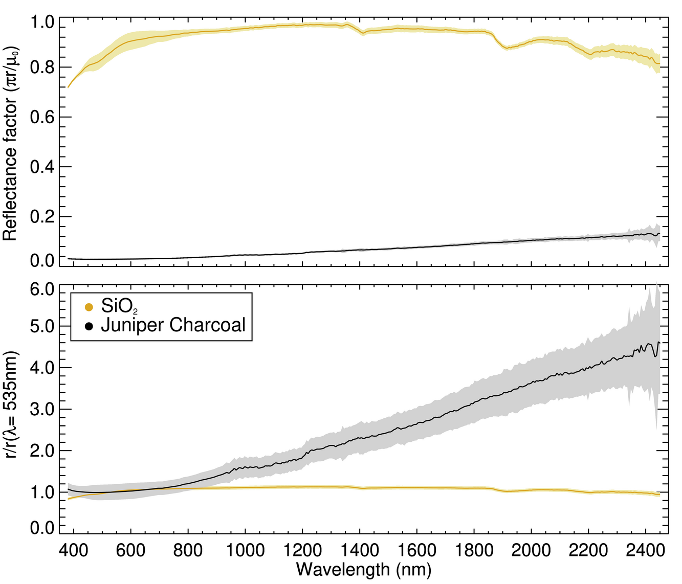
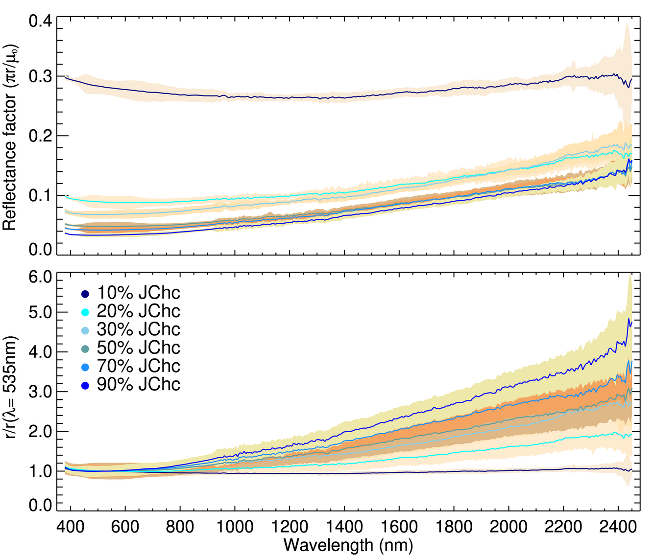
Figure 2: Spectra of both end-members and mixtures measured with MoHIS are plotted above. Each spectrum was acquired near opposition ($\alpha$ $\sim$ 4 to 7${}^{\circ}~{}$) For each spectrum, the propagated dispersion associated to the measurements is depicted by a corresponding filled color envelope around the solid lines. For clarity, only the spectra for the 10%, 20%, 30%, 50%, 70% and 90% juniper charcoal mixtures are displayed in the plots of the right column. – Top plots: Reflectance spectra for the SiO₂ and JChc samples (left) and for Cophylab dust mixtures (right). – Bottom plots: Reflectance spectra normalised at 535 nm for the SiO₂ and JChc samples (left) and for Cophylab dust mixtures (right).

Fig. 2, top-left) shows the extreme contrast between the spectra of SiO₂ and juniper charcoal. The juniper charcoal spectrum presents low REFF values from the visible to the near-infrared (from 0.031$\pm$0.003 at 380 nm through 0.047$\pm$0.007 at 1000 nm to 0.13$\pm$0.06 at 2450 nm), an absence of marked spectral features and a nearly monotonic behaviour. Although the charcoal REFF spectrum marginally decreases to 0.029$\pm$0.007 at 535 nm, it increases readily and steadily from 600 nm onward and across the whole near-infrared domain. These spectral features are consistent with similar carbon-bearing materials (Cloutis et al., 1994; Moroz et al., 1998b; Andrés & Bona, 2005).
Using the spectral slope formula from Fornasier et al. (2015), and adapting for the nearest-neighbours wavelengths, we find that this monotonic behaviour is marked with a stronger spectral slope between 1000 nm and 2400 nm (S $\sim$ 13$\pm$4%/100 nm) than between 380 nm and 1000 nm (S $\sim$ 8$\pm$2 %/100 nm). This behaviour is particularly obvious when the spectrum is normalised at 535 nm (see Fig. 2, lower-left), with the reflectance values in the near-infrared range increasing steadily, to reach over four times the reflectance at 535 nm (REFF_535mn $\simeq$ 0.029$\pm$0.007) at wavelengths longer than 2200 nm.
Moreover, the normalised spectrum highlights the presence of a wide but shallow dip in reflectance ($\sim$ 5% with respect to the surrounding continuum) extending from $\sim$ 1000 nm to $\sim$ 1200 nm. This wavelength range matches the wavelength windows for overtones of the CH_x absorption bands (Lipp, 1992), such as those exhibited by polycyclic aromatic hydrocarbons (e.g. Izawa et al. 2014).

On the contrary, the SiO₂ spectrum exhibits much higher reflectance factor values (see Fig. 2, top-left), and displays several spectral features. The SiO₂ spectrum increases steadily throughout the visible domain (from a REFF value of 0.73$\pm$0.01 at 380 nm to 0.96$\pm$0.02 at 800 nm) and reaches a maximum value of 0.99$\pm$0.02 near 1230 nm, before gradually decreasing to a value of 0.83$\pm$0.07 at 2450 nm.

We interpret this reflectance decrease across the infrared domain as a likely effect of the grain-size distribution of this weekly absorbent particulate medium. Indeed, numerous particles present a diameter smaller than 1$\mu$m in the SEM images, (see Fig. 1). At these wavelengths and for such grain-size, individual particles are expected to diffract light and behave as strong absorbers. However, given the compacity of this SiO₂ particulate medium, the clear presence of agglomerates in the SEM images and the SiO₂’s negligible absorption index in this wavelength range (Kitamura et al., 2007), it is reasonable to assume that part of the medium is in a volume scattering regime in which diffraction is negligible, as clumps of small-than-wavelength particles scatter light in the way a single particle with an equivalent diameter would (Hapke, 1993; Mustard & Hays, 1997; Rousseau et al., 2017).

Furthermore, in the infrared domain, the SiO₂ spectrum displays three dips in reflectance: at $\sim$ 1400 nm ($\sim$ 7143 cm^-1), at $\sim$ 1900 nm ($\sim$ 5263 cm^-1), and at $\sim$ 2200 nm ($\sim$ 4545 cm^-1). These spectral bands are associated with water and/or hydroxyl group from weathering of the sample and/or adsorption of atmospheric water vapor (Elliott & Newns 1971; Lipp 1992; Workman & Weyer 2012, and references therein). Additional spectral measurements were performed after placing the SiO₂ sample in a desiccating oven at 100${}^{\circ}~{}$C at room pressure for 30 hours, in which the spectral features were still present. We note, according to Zhuravlev 2000 and Rahman et al. 2008, that the total removal of -OH and H₂O bound groups from amorphous SiO₂ start to occur from temperatures higher than 150${}^{\circ}~{}$C at room pressure.
Although investigating the water vapor adsorption efficiency of this SiO₂ sample would have been beyond the scope of this analysis, we interpret the continuous presence of these hydration and hydroxylation bands as a likely indication of -OH and H₂O strongly tied to the SiO₂ matrix, both of which might also contribute to the predisposition of the SiO₂ sample to form aggregates.

While some coals and charcoals (e.g. Moroz et al. (1998b), Pommerol & Schmitt (2008)) display hydration and hydroxylation features in their spectra, our JChc sample does not exhibit such spectral features. Although Dias et al. (2016) reports that the water content of a charcoal sample is related to its porosity, Quirico et al. (2016) also points out that the absence of hydration or hydroxylation features in the near-infrared is a sign of charcoal maturity, and a low hydrogen to carbon atoms (H/C) ratio.
Both the studies of Moroz et al. (1998b) and Quirico et al. (2016) highlight, respectively through the examples of the anthraxolites and the anthracite sample PSOC-1468, how the longer a coal goes through a carbonisation process, the greater its carbon content and the lower its overall reflectance become.
Together with the broad reflectance dip across the 1000 – 1300 nm range, we therefore interpreted the absence of distinguishable hydration and hydroxylation features in the juniper charcoal spectrum as a likely indication of an elevated carbon-content and a low H/C ratio.

In order to verify this interpretation, elemental analyses of juniper charcoal samples were performed using a Thermo Scientific FLASH 2000 organic elemental analyser (Brechbühler AG, Schlieren, Switzerland). This instrument, equipped with a reactor consisting of chromium oxide, elemental copper, and silvered cobaltous-cobaltic oxide, allowed to measure the amount of carbon, hydrogen and nitrogen present in the provided samples. Atropine, cystine, and sulphanilamide, provided by Elemental Microanalysis (Okehampton, UK), were used as standards for calibration, while sample quantities in the range of 1-3 mg were weighed for analysis.
Two different samples of juniper charcoal investigated with this instrument contained 80.42$\pm$0.43% of carbon and 2.69$\pm$0.01% of hydrogen, and thus a H/C ratio of $\sim$ 3%. No trace of nitrogen was found. Such a value of H/C is comparable to those of anthraxolites-rich coals, which also present a featureless monotonically increasing spectrum and are generally associated with polyaromatic compounds (Moroz et al. 1998b and references therein).

3.1.2 Intimate mixtures of SiO₂ and juniper charcoal

Similarly, the REFF spectra of the intimate mixtures without and with normalisation at 535 nm have been plotted in Fig. 2 (top- and bottom-right). For better readability, only a selection of the measured spectra is plotted in that figure.
The direct comparison of the pure SiO₂ REFF spectrum (Fig. 2, top-left) with that of the 90% SiO₂/10% JChc mixture (Fig. 2, top-right) clearly shows how the inclusion of a limited amount (by mass) of juniper charcoal drastically affects the reflectance of the mixture: whereas the REFF values of the SiO₂ spectrum were above 0.75 across the considered wavelength range, the 10% juniper charcoal mixture presents REFF values between 0.25 and 0.30 across the same range (i.e. in average a 67$\pm$4% reduction).
However, while compared to the pure SiO₂ spectrum, each increment of juniper charcoal lowers the average REFF value further, the average difference between the spectra of the previous and the new increment decreases. The specific progression at 535 nm, listed in Table 2, can be fitted with an exponential reduction, and is investigated in the discussion section.

Table 2: Variation of the mixtures REFF values and the pure juniper charcoal value with respect to the pure SiO₂ REFF value at 535 nm ($\sim$ 88.5$\pm$0.6%).

Sample	REFF ratio	Sample	REFF ratio
10% JChc	70$\pm$4%	60% JChc	95$\pm$1%
20% JChc	90$\pm$2%	70% JChc	96$\pm$1%
30% JChc	93$\pm$2%	80% JChc	96$\pm$1%
40% JChc	94$\pm$2%	90% JChc	96$\pm$1%
50% JChc	95$\pm$2%	100% JChc	97$\pm$1%

Additionally, these spectra do not exhibit the hydration and hydroxylation spectral features present in the SiO₂ spectrum, even for the mixture containing only 10 wt. % of juniper charcoal. This observation is consistent with the literature (e.g. Pommerol & Schmitt 2008; Jost et al. 2017b; Rousseau et al. 2017). The authors of these studies found that the reflectance properties of a binary mixture composed of both very bright and very dark materials would be dominated by the dark end-member.

The comparison of these spectra with that of juniper charcoal points out that, while mixtures with a charcoal content higher than 10% exhibit a profile akin to that of the pure juniper charcoal sample, the spectrum of the 10% charcoal mixture differs from those of both pure – end-members. The 10% juniper charcoal spectrum follows a shallow u-curve profile, with a marked negative spectral slope between 380 nm and 800 nm (-2.3$\pm$0.2 %/100 nm) and a small positive spectral slope between 1200 nm and 2400 nm (1.0$\pm$0.2 %/100 nm).
The spectra of samples with a larger charcoal content match the trend of the pure juniper charcoal sample, with REFF values slightly decreasing between 400 and 600 nm and then increasing monotonously up to 2450 nm. Furthermore, across the 380 nm – 800 nm range, we note that the mixtures’ spectral slope increases in pair with the juniper charcoal content up to a value of 1.2$\pm$0.4 % /100 nm for the mixture with a JChc mass fraction of 90%. Similarly, the spectral slopes across the 1200 mm – 2400 nm also increase steadily up to 12$\pm$6% / 100 nm for the 90% charcoal mixture, with a trend of 0.21$\pm$0.02 %/100 nm/% of charcoal content.

We interpret the absence of the hydration and hydroxylation bands from the mixtures’ spectra, the rapid overall decrease in reflectance, as well as the progressive matching of spectral slopes across both the visible and the near-infrared range as an further indication of the juniper charcoal fraction controlling the spectroscopic and photometric, and thus more generally the optical properties of the mixtures, as discussed in Rousseau et al. (2017). We therefore interpret the features distinguishing the 10% juniper charcoal spectrum from the other mixtures’ spectra (e.g. the high REFF values and the low spectral slopes values) as the expression of the transition from the SiO₂ fraction driving the optical properties of the mixture to them being controlled by the juniper charcoal fraction.

3.2 Phase curves and photometric modeling

Selections of measured phase curves at 0${}^{\circ}~{}$and 60${}^{\circ}~{}$of incidence are plotted in Fig 3a and 3b, respectively.

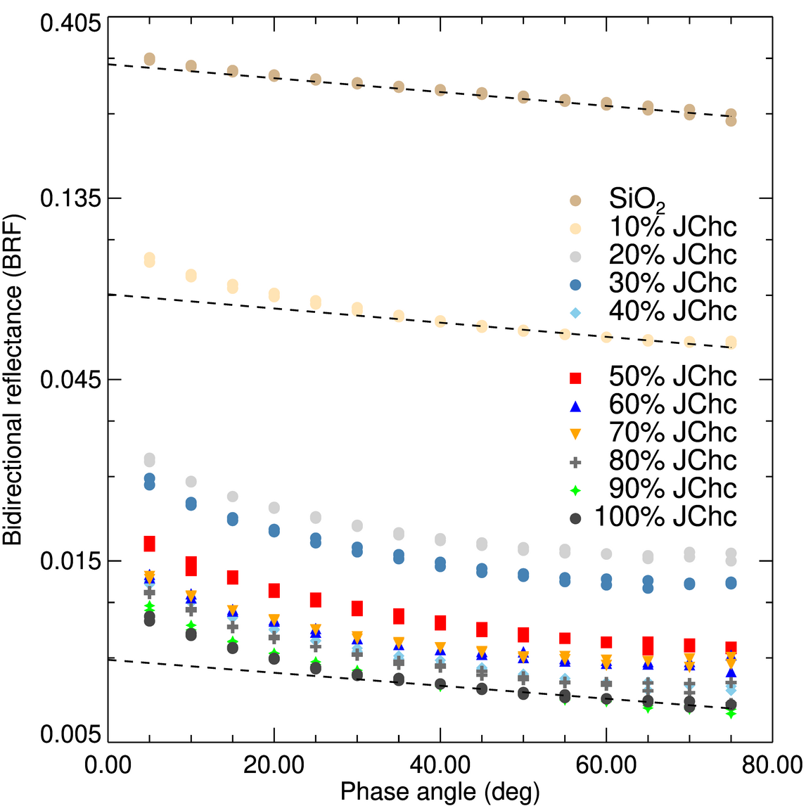
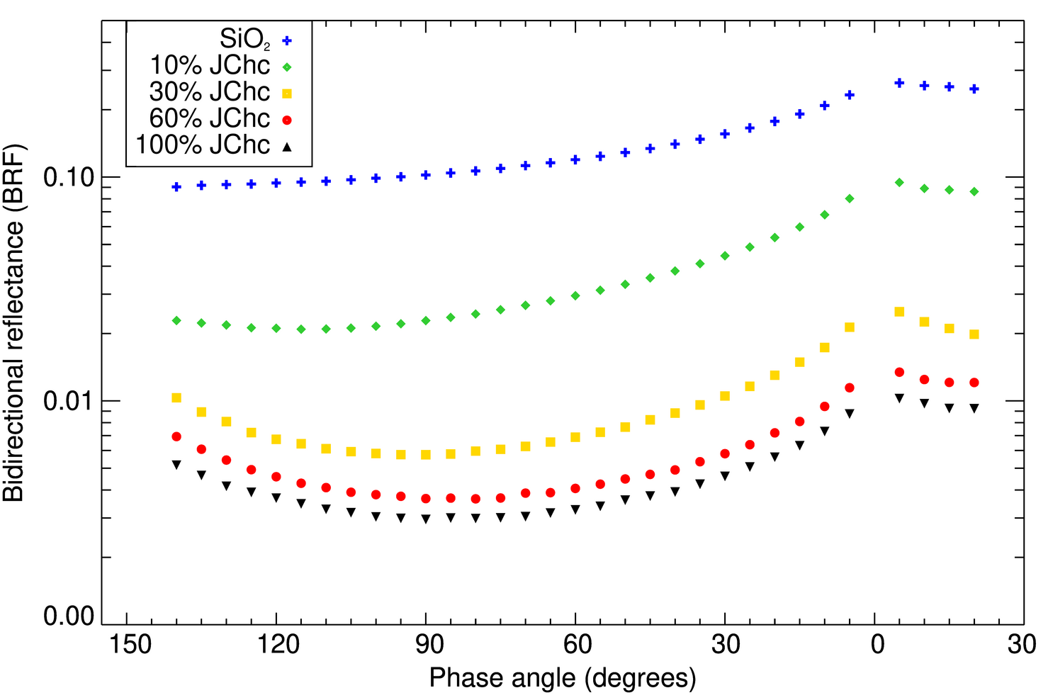
Figure 3: Phase curves of the pure materials and their mixtures at 550 nm, at an incidence angle of 0${}^{\circ}~{}$(left) and 60${}^{\circ}~{}$(right). For clarity, the dispersion of the measurements are not included, and the reflectance axis follows a logarithmic scale. – Left: The black dotted lines plotted over the phase curves of the end members and the 10% JChc mixture are the exponential fits of the 30${}^{\circ}~{}$-75${}^{\circ}~{}$portion of the corresponding curves, and highlight the non-linear surge of the reflectance at low phase angles.

Overall, the phase curves in Fig. 3 show a strong decrease in reflectance with the increase of charcoal content. They also display a non-linear reflectance surge at low phase angles, typically associated to self-shadowing in a particulate medium, also known as the shadow-hiding opposition effect (SHOE, Hapke 1993). In Fig. 3 (left), we note a difference in the magnitude of the departure from linear behaviour between the pure SiO₂ sample and the darker samples, suggesting a difference in the amplitudes of the SHOE affecting each sample.
As discussed previously, we fitted the acquired phase curves at 550 nm and under an incidence angle of 0${}^{\circ}~{}$with the implementation of the Hapke photometric model discussed in section 2.5. Focusing on this part of the dataset has a drawback, as the constraints on the asymmetry factor ($\xi$) and on the photometric roughness ($\bar{\theta}$) are then limited (see e.g. Pilorget et al. 2013 and Labarre et al. 2017). However, to allow direct comparison with the literature (e.g. Li et al. 2013, Fornasier et al. 2015), we ultimately focused on these particular phase curves.

The sets of best-fitting parameters for each sample are listed in Table 3 and the associated quality-fits are presented in fig. 14. We find that while all materials and samples present a back-scattering behaviour, the SiO₂ sample is more back-scattering than the juniper charcoal sample, with its corresponding asymmetry parameter ($\xi_{SiO_{2}}\simeq$ -0.28) being almost twice as large as that of the juniper charcoal ($\xi_{JChc}\simeq$ -0.15). Compared to the literature and assuming no major dependencies of this parameter with wavelength, we find that these samples are slightly less back-scattering than most cometary nuclei, for which the best-fitting values are currently found to be between -0.5 and -0.3 (Ciarniello et al. 2015; Feller et al. 2016; Hasselmann et al. 2017 and references therein).

The contrast between the SiO₂ and the juniper charcoal also appears through the derived parameters of the SHOE function (B_SH,0 and h_SH) which point to two different photometric behaviours near opposition. Both the SiO₂ sample and the 10% charcoal mixture present a moderate reflectance surge (B${}_{SH,0}<$ 1) with peaks having an half-width at half-maximum (HWHM $\simeq 2\cdot$h_SH, Hapke, 1993) smaller than 10${}^{\circ}~{}$, while most mixtures and the pure juniper charcoal sample each exhibit a reflectance surge with a wider peak (HWHM $\simeq$ 10${}^{\circ}~{}$– 17${}^{\circ}~{}$), and a large amplitude (B${}_{SH,0}>$ 1). These two behaviours and the dominant role of the juniper charcoal are consistent with our previous observations of the SiO₂ material being bright and weakly absorbing (thus casting small shadows), while the juniper charcoal is dark and strongly absorbing and thus cast stronger shadows). These results are also consistent with the literature for opaque surfaces (e.g. Shepard & Helfenstein 2007; Shevchenko et al. 2012; Masoumzadeh et al. 2016), on which the SHOE function is the main driver behind their reflectance surge at opposition.

Additionally, the larger-than-one SHOE amplitude are also consistent with the literature on atmosphereless small-bodies (e.g. Helfenstein et al. 1994; Simonelli et al. 1998; Li et al. 2004; Li et al. 2013; Feller et al. 2016). We note indeed that in the canonical description of the Hapke photometric model, the B_SH,0 parameter stands for the amplification of the shadow-hiding phenomenon due to the effect of the size of the scattering particle. However, it is indicated in Hapke (1993) that particles with a complex geometry and their agglomerates are expected to cast shadows on themselves ("self shadowing"), which would be then manifest through values higher than 1. Hence, we interpret the higher-than-one B_SH,0 values to further point to the driving influence of the charcoal given the numerous presence of agglomerates and opaque particles complex shapes as observed in the SEM images.

Considering Helfenstein & Shepard (2011) in the implementation of this photometric model, the width of the SHOE function is tied with the porosity correction factor K and therefore to the superficial porosity of the medium, as described in Hapke (2008). We thus derived the superficial porosity values (P) listed in Table 3 from the best-fitting h_SH values. While slightly higher than the bulk porosities measured with the helium pycnometer (P${}_{SiO_{2}}\simeq$ 65%, P${}_{JChc}\simeq$ 68%), these values theoretically reflect the porosities in the uppermost layers of scatterers. They are consistent with the other measures of this study, with measurements of 67P/CG derived from Rosetta’s optical observations (Fornasier et al., 2015; Hasselmann et al., 2017) or from Philae’s radar (Kofman et al., 2015), and with laboratory experiments on aggregates (Bertini et al., 2007; Lasue et al., 2011).

The photometric roughness describes the average slope of the sample surface in the model, as perceived below the spatial resolution of the detector (at the centimetre scale given the setup of these measurements). The best-fit values are $\bar{\theta}\simeq$ 4${}^{\circ}~{}$-11${}^{\circ}~{}$. These values are slightly lower than the retrieved photometric roughnesses of visited cometary nuclei observed at larger spatial resolutions (e.g. $\bar{\theta}_{81P/Wild-2}\simeq$ 15${}^{\circ}~{}$, Li et al. 2013), and than the global and local roughnesses found for 67P/C-G (between 15${}^{\circ}~{}$and 33${}^{\circ}~{}$, see Fornasier et al. 2015; Feller et al. 2016; Hasselmann et al. 2017). However, these values as such are consistent with loose and smooth-surfaced particulate media with grain sizes between 0.1 and 50 $\mu$m investigated in laboratory settings (Shepard & Helfenstein, 2007).

Table 3: List of best-fitting parameters for the HHS photometric model (averaged over the best 500 solutions) and associated dispersion. See Table 1 for a description of each model parameter. The porosity (P) is derived from the porosity coefficient K. $\chi^{2}$ and R² standing respectively as the normalised root-mean-square deviation and the Pearson coefficient. A_geo and A_bd respectfully corresponds to the geometrical and bidirectional albedos computed from the associated best-fitting parameters.

Samples	$\omega_{ssa}$	$\xi$	BSH,0	hSH	$\bar{\theta}$ (deg)	P (%)	$\chi^{2}$ (x10-3)	R2	Ageo	Abd
Pure SiO2	0.975$\pm$0.1	-0.276$\pm$0.003	0.59$\pm$0.02	0.07$\pm$0.01	5.$\pm$1.	87.$\pm$1.	2.070	0.994	1.07$\pm$0.01	83.2$\pm$0.9
10% charcoal	0.478$\pm$0.3	-0.241$\pm$0.002	0.90$\pm$0.01	0.09$\pm$0.01	$<$ 5.*	83.$\pm$1.	0.595	0.997	0.34$\pm$0.01	23.4$\pm$0.3
20% charcoal	0.139$\pm$0.2	-0.178$\pm$0.003	1.61$\pm$0.03	0.11$\pm$0.01	6.$\pm$1.	79.$\pm$1.	0.176	0.997	0.11$\pm$0.01	6.4$\pm$0.1
30% charcoal	0.117$\pm$0.1	-0.186$\pm$0.001	1.64$\pm$0.01	0.11$\pm$0.01	4.$\pm$1.	79.$\pm$1.	0.231	0.995	0.09$\pm$0.01	5.5$\pm$0.1
40% charcoal	0.062$\pm$0.2	-0.190$\pm$0.006	1.57$\pm$0.09	0.13$\pm$0.01	6.$\pm$1.	76.$\pm$1.	0.083	0.998	0.05$\pm$0.01	2.9$\pm$0.2
50% charcoal	0.09$\pm$0.1	-0.217$\pm$0.002	1.24$\pm$0.02	0.09$\pm$0.01	4.$\pm$1.	82.$\pm$1.	0.169	0.994	0.06$\pm$0.01	3.8$\pm$0.1
60% charcoal	0.076$\pm$0.2	-0.165$\pm$0.006	1.44$\pm$0.05	0.11$\pm$0.01	7.$\pm$1.	79.$\pm$1.	0.141	0.993	0.05$\pm$0.01	3.3$\pm$0.1
70% charcoal	0.076$\pm$0.1	-0.171$\pm$0.002	1.33$\pm$0.03	0.11$\pm$0.01	$<$ 5.*	78.$\pm$1.	0.099	0.996	0.050$\pm$0.009	3.4$\pm$0.1
80% charcoal	0.063$\pm$0.2	-0.180$\pm$0.008	1.46$\pm$0.08	0.12$\pm$0.01	10.$\pm$1.	77.$\pm$2.	0.147	0.992	0.046$\pm$0.008	2.8$\pm$0.2
90% charcoal	0.057$\pm$0.2	-0.179$\pm$0.007	1.49$\pm$0.08	0.12$\pm$0.01	9.$\pm$1.	76.$\pm$1.	0.076	0.997	0.042$\pm$0.005	2.5$\pm$0.2
Pure charcoal	0.056$\pm$0.3	-0.155$\pm$0.006	1.40$\pm$0.05	0.15$\pm$0.01	11.$\pm$2.	73.$\pm$2.	0.070	0.997	0.038$\pm$0.002	2.5$\pm$0.2
9P/Tempel 11	0.039$\pm$0.005	-0.49$\pm$0.02	[1]	[0.01]	16$\pm$8	-	-	-	0.056	0.013
67P/C-G2	0.026$\pm$0.001	-0.42$\pm$0.02	2.56$\pm$0.067	0.067$\pm$0.005	16.3$\pm$0.2	85.	-	-	0.052	-
Average C-type3	0.025	-0.47	1.03	0.025	20	-	-	-	0.049	-
Deimos4	0.079$\pm$0.002	-0.29$\pm$0.03	1.6$\pm$0.6	0.07$\pm$0.3	16.4	-	-	-	0.067$\pm$0.007	0.027$\pm$0.003
Phobos4	0.054	-0.13	5.7	0.072	22	-	-	-	0.071$\pm$0.012	0.021$\pm$0.004

*: Upper limit of the subset of optimal solutions.

1: Li et al. (2007), parameters at 550 nm (with B_SH,0 and h_SH fixed); 2: Feller et al. (2016), parameters at 535 nm;

3: Helfenstein & Veverka (1989), parameters in the V band; 4:Thomas et al. (1996); Simonelli et al. (1996), parameters at 540 nm.

4 Discussion

4.1 Influence of the dark end-member

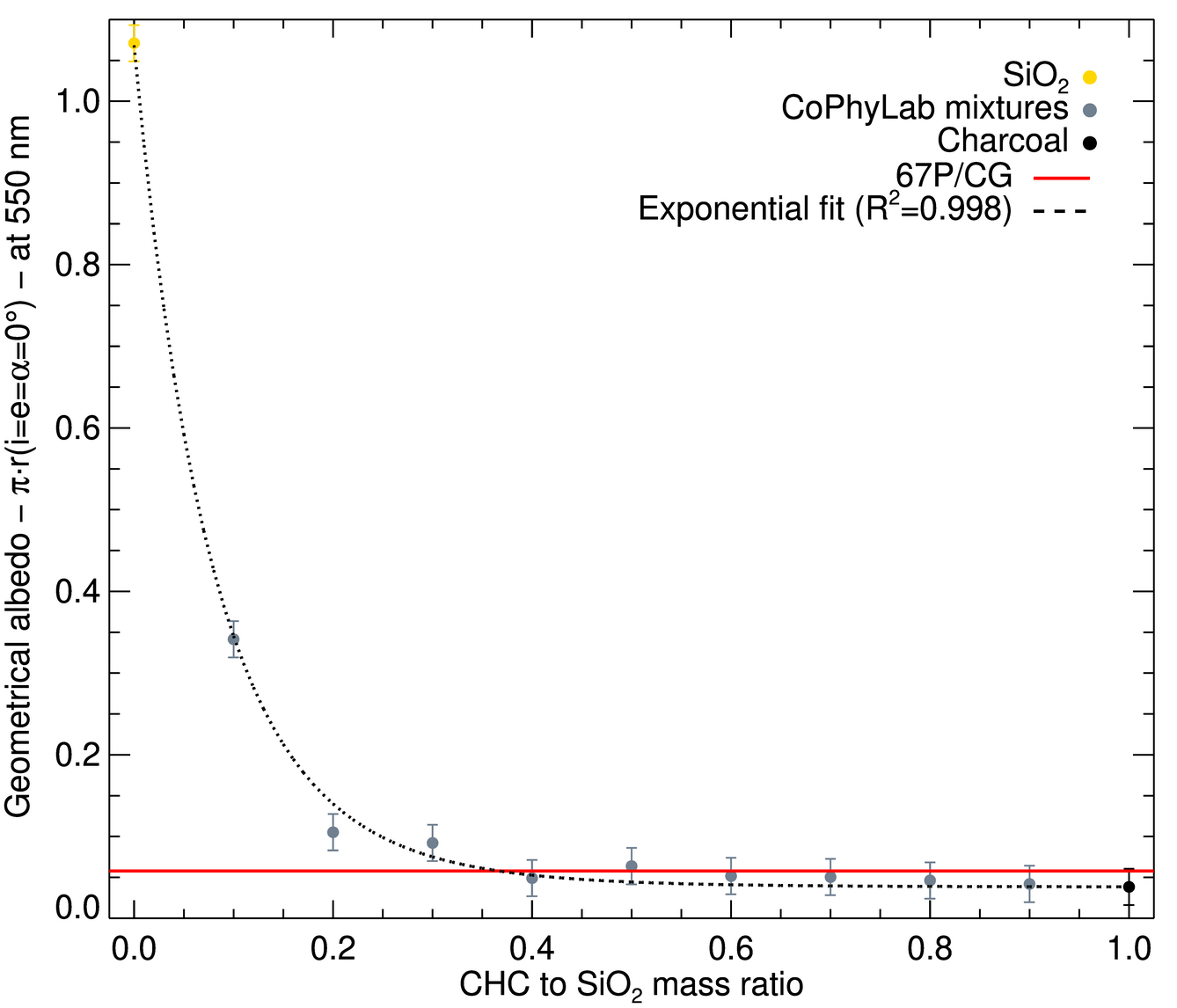
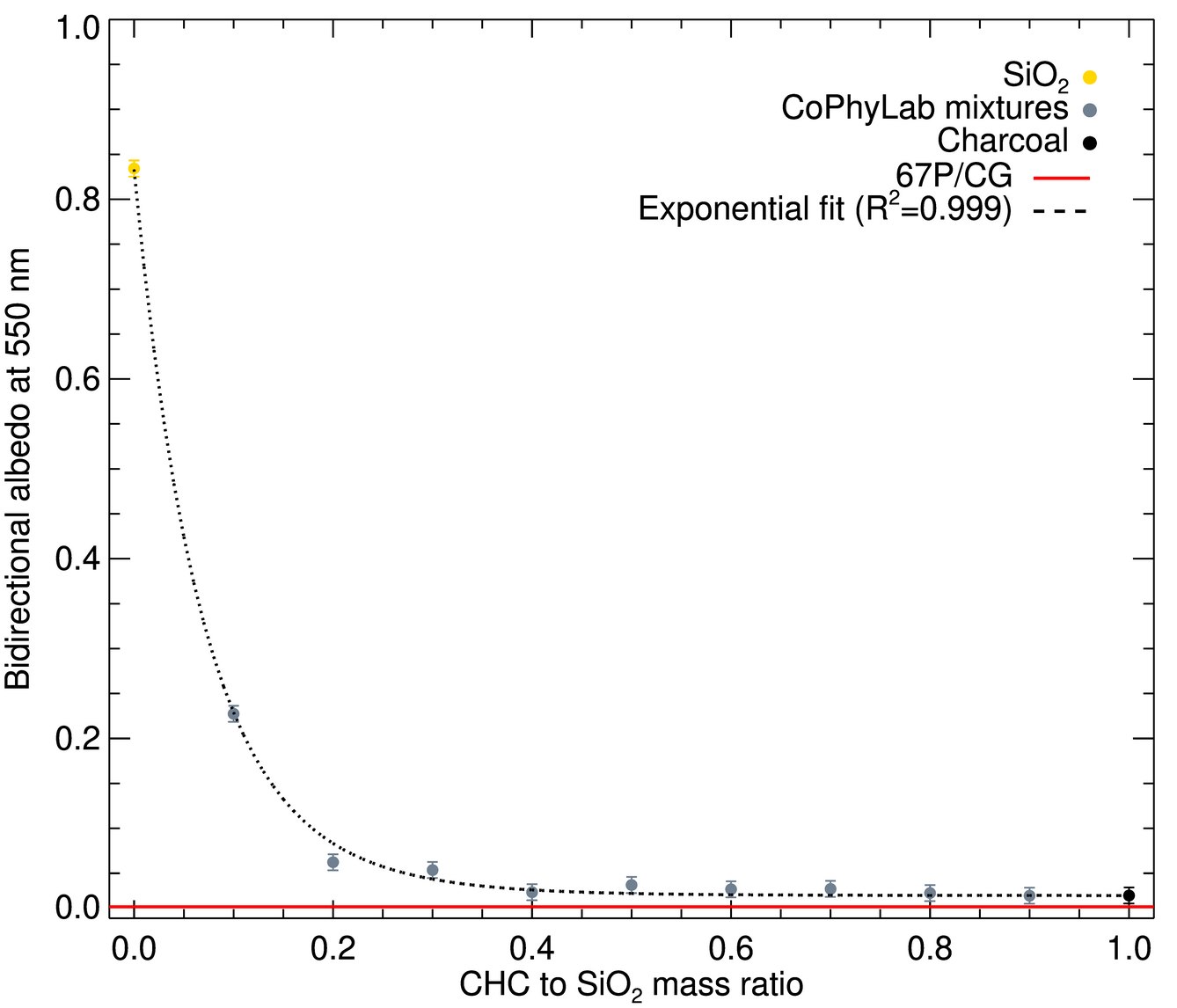
Figure 4: Left: Geometric albedos values for the CoPhyLab dust mixtures and its end-members. – Right: Bidirectional albedos values for the CoPhyLab dust mixtures and its end-members. – As illustrated in both plots, the strong albedo decreases are best fitted with simple exponential functions (black dashed lines). The red line stands for the corresponding albedo of 67P/Churyumov-Gerasimenko’s nucleus at 550 nm (Fornasier et al., 2015).

As detailed throughout the Results section, both spectroscopic and photometric measurements point to the prominent role of the ground juniper charcoal in the resulting optical properties of the CoPhyLab dust mixtures. This observation is in agreement with the literature (e.g. Warren & Wiscombe 1980; Clark & Lucey 1984; Pommerol & Schmitt 2008; Yoldi et al. 2015). In each of these studies, the authors found that for mixtures of bright and dark materials, the inclusion of a fraction of the dark end-member was sufficient to strongly reduce the overall brightness of the mixture. Using $\mu$m-sized particles, Cloutis et al. (2015) reported specifically that such decrease is more intense for intimate mixtures than for areal mixtures. Furthermore, Rousseau et al. (2017) has shown that this decrease was also observed when mixing sub-$\mu$m-sized particles. The originality here, further discussed in the rest of this section is that we are in principle in the opposite configuration where the particles of the dark material are much bigger in size than the individual particles of the bright material.

Both Jost et al. (2017b) and Rousseau et al. (2017) discussed the mechanisms of such reflectance decreases in either the context of icy or non-icy mixtures. In the case of intimate mixtures of $\mu$m-sized water-ice and activated charcoal, Jost et al. (2017b) reported that the variations of the hemispherical albedos appeared to follow an exponential decrease as the amount of activated charcoal was increased.
We list in Table 3 the bidirectional and geometric albedo values plotted in fig. 4. Similarly to these two studies, we also find that their progression can be satisfactorily fitted with an exponential function of the type albedo = albedo${}_{\text{JChc}}$+$e^{\left(a+b\cdot(1+\omega_{\text{JChc}})\right)}$, with $\omega_{\text{JChc}}$ the mass fraction of the charcoal. For the geometric albedo values, the best set of fitting parameters (a, b) was found to be equal to (0.03 $\pm$0.01,-12.7 $\pm$0.1) and in the case of the bidirectional albedo to (-0.21 $\pm$0.01, -14.5 $\pm$0.1).
Considering the albedo values of Table 3, and given the best-fitting parameters, we find that all mixtures with at least 40% of charcoal by mass present a geometrical albedo close to or lower than that of 67P/C-G’s nucleus (A${}_{geo,550nm}\simeq$ 5.9$\pm$0.3%).

4.2 Cross-sectional scattering efficiencies and surface heterogeneities

Although the effective grain-size distribution of particles at the surface of comet 67P/C-G has not been characterized all across the nucleus, the physical properties of both ice and dust fractions have been investigated. Freshly exposed water-ice-enriched material was found to be best reproduced with micrometric to millimetric water-ice grains (e.g. De Sanctis et al. 2015; Filacchione et al. 2016; Raponi et al. 2016). Ejected dust particles in the inner coma were investigated both remotely with the spectrometer VIRTIS and under the microscope with the instrument MIDAS. Bockelée-Morvan et al. (2017) and Mannel et al. (2019) notably reported the observations of sub-micrometric to micrometric-sized dust grains and aggregates. Rousseau et al. (2017) found, through laboratory experiments, a satisfactory match for 67P/C-G’ spectral properties in the visible domain, by mixing sub-micrometric grains of mature coal, pyrrhotite, and dunite.
Further laboratory measurements presented in Jost et al. (2017a) showed that the sublimation residues of micrometric particles of activated charcoal coated with water-ice (a type of intimate mixture they refer to as "intra-mixture") possessed phase curves that closely resembled the phase curve of the Apis/Imhotep border, measured during the low-altitude low-phase angle flyby of 67P’s nucleus (Feller et al., 2016).
Moreover through the modeling of the scattering properties of the dust particles from the nucleus and the inner coma, Marschall et al. (2020) showed that the dust phase function of the inner coma was best-fitted by particles ranging in the tens of micrometres, while the phase function of the nucleus could be fitted with a model of larger particle aggregates ($>$ 100 $\mu$m).

As specified in Lethuillier et al. (2022), the CoPhyLab dust mixture was also designed to replicate the range of particle sizes found for 67P/C-G. On the one hand, the chosen SiO₂ material is composed of sub-micrometric and micrometric particles, as mentioned above in Sec. 2. In particular, for this industrially manufactured material, Kothe et al. (2013) reported a mean particle-size of 0.63 $\mu$m by count, and of 2.05 $\mu$m by mass. Such sizes are consistent with the SEM images of our sample (see Fig. 1). Moreover, this material has also a propensity to form aggregates sizing up to the millimetre.
On the other hand, our juniper charcoal material was grinded then sieved with a 50 $\mathrm{\mu}$m mesh and Lethuillier et al. (2022), resolving optically juniper charcoal particles suspended in an ethanol solution, found an average particle-size of $\sim$ 24 $\mu$m.

As a cross-verification of the characterization of the materials, we considered the spectral mixing relation given in Hapke (1993) between physical quantities and single-scattering albedoes for intimate mixtures of closely-packed particulates. Assuming that the i^th group of particles from the mixture contains N_i particles, of cross-section $\sigma_{i}$ associated with the extinction efficiency Q_E,i, and the single-scattering albedo w_i, Hapke (1993) states:

$$w_{mixture}=\left(\sum_{i}N_{i}\sigma_{i}\cdot w_{i}Q_{E,i}\right)/\left(\sum_{j}N_{j}\sigma_{j}\cdot Q_{E,j}\right)$$ (4)

In the particular case of an ideal binary mixture for which all particles of either material have a quasi-spheroidal shape with an equivalent diameter D_i that is larger than wavelength, the Fraunhofer diffraction is negligible (i.e. Q_E,i $\sim$ 1) according to Bohren & Huffman (1983), and Hapke (1993) simplifies Eq. 4 as follows:

$$w_{mixture}=\frac{x\cdot w_{1}+(1-x)\cdot\zeta\cdot w_{2}}{1+\zeta}~{}~{}\text{where}~{}\zeta=\frac{M_{2}}{\rho_{2}D_{2}}\cdot\frac{\rho_{1}D_{1}}{M_{1}}$$ (5)

where M_i and $\rho_{i}$ are respectively the bulk and the apparent particle densities for the i^th material, and x the mass fraction of the first material.

Using that last equation and the values determined previously for either material, we plotted the generated curve for all mass fractions against the determined single-scattering albedoes for each prepared mixture (respectively the orange line and the black points) in Fig. 5.

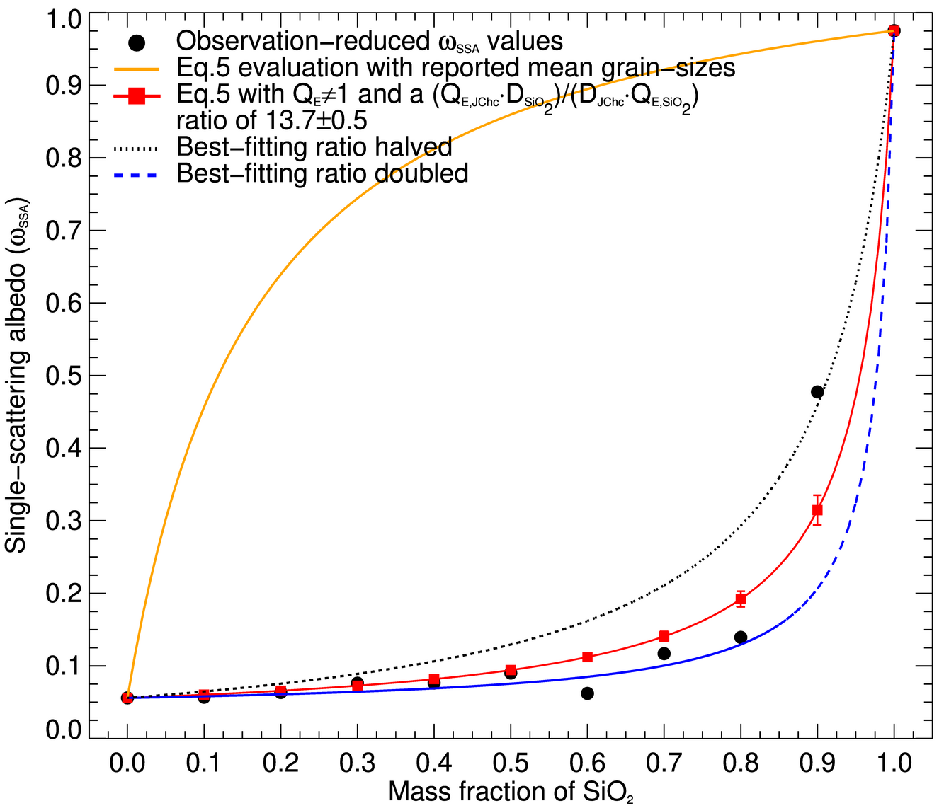
Figure 5: Single-scattering albedo (SSA) values for SiO₂, juniper charcoal, and the considered intimate mixtures. In this figure, non-visible error-bars are hidden by the plot symbols. This plot highlights the discrepancy between the SSA values derived from the PHIRE2 measurements (black circles) and those computed directly with Eq. 5 using the end-members’ reported mean grain-sizes (2.05 $\mathrm{\mu}$m for the SiO₂ and 24 $\mathrm{\mu}$m for the JChc) and assuming their particles to be equant (orange line). The divergence of the SSA values for mass fractions 0.6 and 0.9 is further discussed in the main text.

We note here that for the benefit of clarity, we only generated the said curve using a SiO₂ mean grain-size of 2.05 $\mathrm{\mu}$m , which provided the closest result to the SSA values from either reported grain-size.
The mismatch between the curve drawn from Eq. 5 and the SSA values is evident. Under the hypotheses upholding this equation, the grain-sizes ratio of the two materials would have to be inverted for the curve to start matching the SSA values.

A close consideration of the end-members’ SEM images suggest that the discrepancy stems from the hypothesis that the materials’ particles are equant and each of the same size. While the SiO₂ particles present an ample yet limited particle-size distribution, the JChc particles exhibit an wider particle-size distribution (from a few hundred of nanometres to hundreds of micrometre) and a large diversity of shapes. The presence of long needle-like particles (see Fig. 9) is especially of note. Indeed, Zerull (1976) and Bohren & Huffman (1983) demonstrated that the scattering properties of non-equant spheroidal particles differ significantly from those of spherical particles, and the associated simplifications leading to Eq. 5 are therefore unsuited under such premises.

However, for the sake of the argument, if one considers Eq. 5 minus the assumption that Q_E,i = 1 and thus adjusts a $\frac{Q_{E,JChc}\cdot D_{SiO_{2}}}{D_{JChc}\cdot Q_{E,SiO_{2}}}$ ratio with an ordinary least-squares method to fit the SSA values, one finds the best-fitting numerical value to be equal to 13.7$\pm$0.5, for a quality of fit slope of 0.98±0.02 and a coefficient of determination (R²) of 0.99.
The associated curve is displayed in Fig. 5 as a red line with red squares to highlight the computed values corresponding to the mass fractions of the different mixtures.
While this curve is well adjusted to mixtures with a lower mass-fraction of SiO₂, it mismatches determined SSA values for mixtures with a predominant SiO₂ fraction, which could have been interpreted under the premises of Eq. 5 as a difference in terms of grain-sizes in between the mixtures or in terms of scatterers.

While each investigated sample appears to have a homogeneous texture at the millimetre-scale under the naked eye (see Fig. 13), the SEM images present a different picture. As mentioned previously, both end-members (Fig. 1) present wide grain-size distribution, both materials contain sub-micrometric and micrometric particles. In particular, we observe individual SiO₂ particles that are around one or two times the size of the considered wavelength (550 nm) and also find individual juniper charcoal particles or their surface elements that are $\sim$ 10 times smaller (see Figs. 1 (bottom-panel) and 9).
Thus, both materials contain grains and surface elements, whose diameter (or size) is of the order or even smaller than the wavelength (550 nm). Such features will likely act as Rayleigh scatterers and absorbers, and either contribute to increase or decrease the overall reflectance of the material (Hapke, 1993).

Moreover as illustrated in Fig. 12, in every mixture investigated with the SEM, we note the presence of large and compact SiO₂ agglomerates with sizes ranging up to the hundreds of micrometers. If any degree of electromagnetic coupling exists between particles of such agglomerates, then they would interact with incident light similarly to an individual particle of larger size (Mustard & Hays, 1997; Rousseau et al., 2017; Pommerol & Schmitt, 2008).

The SEM of the mixtures images present a more complex picture, especially those with SiO₂ mass fractions higher than 0.5. In particular, for the 90% SiO₂/10% juniper charcoal mixture, several larger charcoal particles are visible at the surface, some of them appearing as inclusions within large SiO₂ agglomerates. For mixtures with a slightly higher charcoal content, such textural heterogeneities are also noticeable with the continuous presence of SiO₂ aggregates noted previously, but also with some juniper charcoal material appearing as loose elements forming a surface surrounding or partially covering the SiO₂ aggregates.

Thus we interpret the mismatch between the results of the spectral mixing model and the SSA values to reflect not only that the end-members are composed of particles with a diversity of shapes but also as a likely consequence of the combination of micro-scale compositional heterogeneities as well as grain-size effects.

We note here that recent researches have investigated the scattering properties of irregular particles, for instance through the generation of 3D particle shapes and the resolution of the T-matrix for these shapes (e.g. Petrov et al. 2012, Grynko et al. 2018). This method has been considered to investigate the properties of 67P/C-G’s coma and nucleus particles. With equant irregular rough agglomerates of sizes ranging from 5 $\mu$m to 100 $\mu$m, and composed of an intimate mixture of strongly opaque nanometre-sized particles and weakly absorbent particles larger in size (up to the micrometre), Markkanen et al. 2018 matched phase curves of the nucleus and the coma of 67P/Churyumov-Gerasimenko. These results underline the usefulness of materials with an extended size-distribution. Moreover, and together with the results presented in this study, they urge for further investigation of non-homogeneous agglomerates composed of particles of varied shapes and sizes.

4.3 Colours and spectral slopes: comparison with small bodies of the Solar System

4.3.1 The case of 67P/Churyumov-Gerasimenko: spectral slopes and colours

The nucleus of comet 67P/CG is to date the most extensively characterised cometary surface. In particular, although the spectrophotometric properties of the nucleus were found to be overall homogenous across both of its lobes, its surface displayed a definite diversity of spectral slopes and albedos correlated to varied compositional and morphological features, e.g. Barucci et al. (2016), Ciarniello et al. (2016), Filacchione et al. (2016), Fornasier et al. (2016), Hasselmann et al. (2016), Oklay et al. (2016), Ferrari et al. (2018), Feller et al. (2019), Fornasier et al. (2019), and Hoang et al. (2020).
Among other results, these studies notably established that three spectrophotometricaly different types of terrains could be identified across the nucleus’ surface: those with a shallow spectral slope (S_882nm-535nm $\simeq$ 11–14 %/100 nm at $\sim$ 50${}^{\circ}~{}$, using a revised definition of Delsanti et al. (2001)), those with a spectral slope between 14 %/100 nm and 18 %/100 nm, and finally those with a spectral slope above 18 %/100 nm, at $\sim$ 50${}^{\circ}~{}$(see Fornasier et al. 2016 for a discussion on the 67P/CG’s nucleus phase reddening). While the first group of terrains was correlated with surfaces and locations presenting an enhanced water-ice content, the third one was associated with water-ice depleted and macroscopically rough surfaces (e.g. boulder fields, escarpment ridges). Finally, the second group of terrains stood out as the typical dust-covered macroscopically smooth expanses present on both lobes of the nucleus.

Using the definition of Fornasier et al. (2015) and the OSIRIS/NAC filter profiles, the corresponding spectral slopes for the CoPhyLab materials and mixtures were estimated for a phase angle of $\sim$ 0${}^{\circ}~{}$and gathered in Table 4). These values maintain the previously noted trend of a 535 nm – 882 nm spectral slope increase with an increasing amount of juniper charcoal content, as well as the observation that overall these visible spectral slopes are weaker than that of 67P/CG. However, assuming the two extreme values found for the phase reddening slope of the 67P/C-G nucleus from either observations acquired around August 2014 or around April-August 2015 (Fornasier et al. 2015; Fornasier et al. 2016 supl. mat.), the spectral slope offset would be either of $\sim$ 2. %/100 nm or of $\sim$ 5. %/100 nm.
Hence, should any compositional differences be set aside, then the spectral slope values of the CoPhyLab mixtures are in appearance consistent with the spectral slopes of the water-ice enriched terrains observed on the surface of comet 67P/CG. However, if the slope offset associated with the phase reddening phenomenon is included, spectral slopes of mixtures with a relative juniper charcoal content above 80% are then comparable with those measured for the dust covered areas such as Anuket or Ma’at on 67P/CG’s nucleus El-Maarry et al. (2015).

Table 4: Visible spectral slope of the pure materials and their mixtures using the same formula from Fornasier et al. (2015), and BVRI colours computed using the canonical Bessell filters. The uncertainties on the charcoal content for the mixtures were evaluated during the sample preparation process. Both analogue or corresponding values available for cometary nuclei flown-by are also listed here for reference.

Sample	535–882 nm slope	B-V	V-R	V-I
(charcoal content)	(%/100 nm, @0${}^{\circ}~{}$)	(mag)	(mag)	(mag)
0% (Pure SiO2)	2.8$\pm$0.2	0.75$\pm$0.03	0.41$\pm$0.01	0.77$\pm$0.03
10.0$\pm$0.02%	-1.4$\pm$0.2	0.61$\pm$0.03	0.34$\pm$0.02	0.65$\pm$0.03
20.0$\pm$0.03%	1.0$\pm$0.3	0.6$\pm$0.1	0.35$\pm$0.04	0.7$\pm$0.1
30.0$\pm$0.05%	3.8$\pm$0.9	0.63$\pm$0.06	0.39$\pm$0.01	0.78$\pm$0.06
40.0$\pm$0.07%	5.0$\pm$1.	0.63$\pm$0.1	0.40$\pm$0.05	0.8$\pm$0.1
50.0$\pm$0.09%	4.0$\pm$1.	0.6$\pm$0.2	0.38$\pm$0.08	0.8$\pm$0.3
60.0$\pm$0.1%	5.0$\pm$1.	0.62$\pm$0.04	0.39$\pm$0.03	0.80$\pm$0.04
70.0$\pm$0.1%	5.0$\pm$1.	0.6$\pm$0.1	0.39$\pm$0.02	0.8$\pm$0.1
80.0$\pm$0.1%	11.0$\pm$3.	0.7$\pm$0.1	0.46$\pm$0.06	0.9$\pm$0.1
90.0$\pm$0.2%	7.0$\pm$2.	0.64$\pm$0.07	0.41$\pm$0.01	0.85$\pm$0.07
100% (Pure JChc)	10.0$\pm$3.	0.6$\pm$0.1	0.42$\pm$0.07	0.9$\pm$0.1
1P/Halley1	[17.4$\pm$0.3]	0.72$\pm$0.04	0.41$\pm$0.03	0.80$\pm$0.07
9P/Tempel 12	[12$\pm$1]	0.84$\pm$0.01	0.50$\pm$0.01	0.99$\pm$0.02
67P/CG3	[11$\pm$2]	0.83$\pm$0.08	0.54$\pm$0.05	1.00$\pm$0.07
67P/CG4	[ 20 ]	0.73$\pm$0.07	0.57$\pm$0.03	1.06$\pm$0.05
103P/Hartley 25	[ 7$\pm$3]	0.75$\pm$0.05	0.43$\pm$0.04	0.84$\pm$0.05

Notes: 1: Thomas & Keller (1989); Lamy et al. (2004), this spectral slope is estimated there between 440 nm and 813 nm at small phase angles. – 2: Li et al. (2007), this spectral slope was estimated there between 310 nm and 950 nm at 63${}^{\circ}~{}$of phase angle. – 3: Tubiana et al. (2008, 2011), this spectral slope was estimated between 436 nm and 797 nm at phase angles lower than 10${}^{\circ}~{}$. This particular set of values was derived from ground-based observations at heliocentric distances larger than 4.5 au, while no coma features were detected. – 4: Ciarniello et al. (2015), this spectral slope was estimated between 550 nm and 800 nm. – 5: Li et al. (2013), this spectral slope was computed between 400 nm and 850 nm, at 85${}^{\circ}~{}$of phase angle.

Although this phase reddening phenomenon has been observed for the Moon’ surfaces (Gehrels et al., 1964), and those of asteroids and meteorites (e.g. Sanchez et al. 2012; Fornasier et al. 2020 and references therein), the mechanisms behind phase reddening are still the subject of studies. This linear increase of spectral slopes with the phase angle has been associated with physical properties such as particle single-scattering, and sub-micron roughness of the regolith Grynko & Shkuratov (2008); Schröder et al. (2014); Ciarniello et al. (2020). In the case of comet 67P/C-G, Fornasier et al. (2016) further associated variations of the phase reddening with compositional changes of the surface as the comet passed through perihelion.

4.3.2 The case of 67P/Churyumov-Gerasimenko: a look at the spectrum

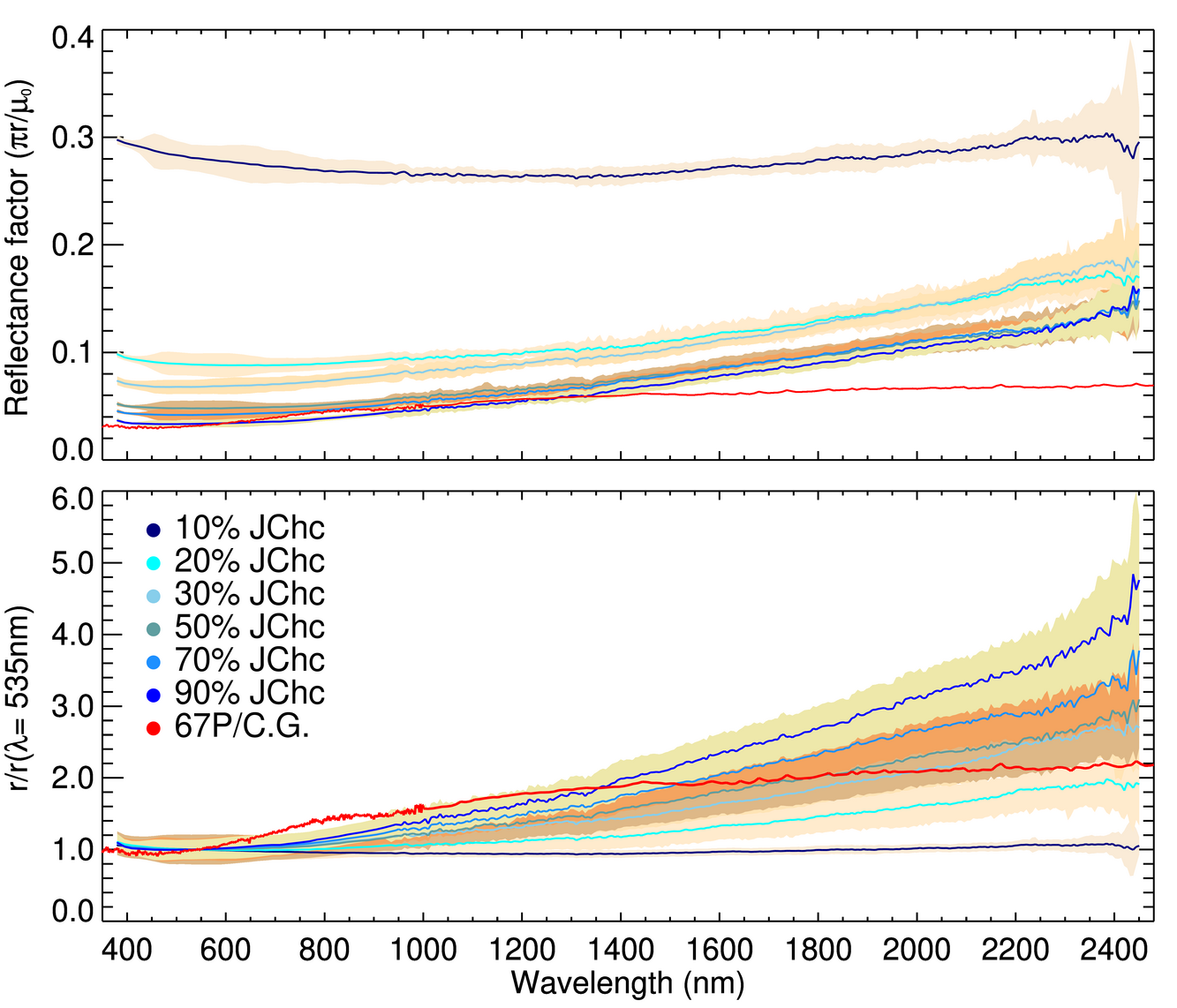
Figure 6: Spectra of the investigated end-members and associated mixtures plotted alongside the spectrum from the Aswan terrace on 67P/C-G (adapted from Capaccioni et al. 2015, and depicted by the solid red curves in this figure). As in Fig. 2, the color filled envelope around the solid curves correspond to the associated dispersion, and only the spectra for the 10%, 20%, 30%, 50%, 70% and 90% juniper charcoal mixtures are displayed for clarity. – Top plots: REFF spectra for the end-members (left) and for the associated intimate mixtures (right). – Bottom plots: Associated reflectance spectra normalised at 535 nm the end-members (left) and for the associated intimate mixtures (right).

Beyond the comparison of colours and spectral slopes in the visible domain, we sought to compare our VIS-NIR spectra with one from a typical surface of 67P/C-G’s nucleus. We plot in Fig. 6 the spectrum from part of the dust-covered terrace overhanging the Aswan cliff near the neck of the comet (Capaccioni et al., 2015; Pajola et al., 2016).
For the purpose of this study, we convert this spectrum given in radiance factor (RADF) in Capaccioni et al. (2015) to reflectance factor (REFF). Using the reconstructed trajectory of Rosetta at the moment of the observation (Acton et al., 2018) and a shape model of the comet (Preusker et al., 2017), we determined that the incidence, emergence and phase angles were respectively of 57$\pm$4${}^{\circ}~{}$, 86$\pm$4${}^{\circ}~{}$, and 28.95$\pm$0.03${}^{\circ}~{}$for this part of the terrace.

As discussed in Capaccioni et al. (2015), this spectrum does not exhibit specific spectral features across the 380 – 2500 nm range and presents a steady low reflectance (from $\sim$ 0.03 at 380 nm and 535 nm to $\sim$ 0.07 at 2500 nm). Compared to the SiO₂ spectrum, both the juniper charcoal and this 67P/C-G spectrum are strikingly darker. However, although these two spectra exhibit comparable low REFF values across the 380 – 1200 nm interval, the juniper charcoal’ spectrum keeps on increasing toward higher wavelengths, reaching up to almost twice the REFF values of 67P/C-G’s beyond 2400 nm (see Fig. 6, top-left). This difference of behaviour in the near-infrared domain is particularly evident in the normalised reflectance plot (Fig. 6 bottom-left), across which 67P/C-G’ normalised reflectance values are plateauing toward 2.1. On the other hand, the JChc normalised spectrum increases steadily from $\sim$ 1.8 at 1200 nm to $\sim$ 4.6 at 2400 mm.
This plot also casts light on the differences between 67P/C-G’s and JChc’ spectra in the visible domain, and in particular across the 535 nm to 800 nm interval over which the spectral slope for 67P/C-G is of 12 %/ 100 nm, whereas the corresponding slope for the juniper charcoal is of $\sim$ 6$\pm$5 %/ 100 nm. This difference in behaviour extends beyond the visible domain with the noted steady increase of the JChc’ relative reflectance, while the 67P/C-G’ relative reflectance spectrum inflects past $\sim$ 800 nm, and then slowly increases from $\sim$ 1.5 to $\sim$ 2.1 (reached at 2450 nm).
We note here that as the 67P/C-G’ spectrum inflects towards this slow-raising segment, together with the juniper spectrum, both spectra present comparable reflectance factor values across the 1000 – 1200 nm interval. Hence, although the 67P/C-G and juniper charcoal spectra exhibit overall different behaviours, across the 380 – 535 nm and 1000 – 1200 nm intervals, the juniper charcoal REFF spectrum presents comparable values to those of the 67P/C-G’ REFF spectrum of a dust-covered area of the nucleus’ surface.

While transitioning from a SiO₂-fraction dominated mixture to a juniper charcoal fraction dominant one, the spectra of these intimate mixtures show shapes that differ significantly from that of 67P/C-G’s nucleus. Both the reflectance factor and the relative reflectance plots of Fig. 6 (right column) illustrate this mismatch across the 400 nm – 2450 nm range. The REFF plot (Fig. 6, upper-right) highlights that only spectra of mixtures with more than 50% of juniper charcoal partially match or have reflectance factor values close to those of this 67P/C-G’ spectrum, over the 400 nm – 1300 nm interval. However, similarly to the pure juniper charcoal spectrum, these same spectra exhibit a continuous increase of their reflectance above 1400 mm, while this 67P/C-G spectrum does not reach REFF values above 0.075.
Additionally, although the relative reflectance plot (Fig. 6, lower-right) highlights that all spectra of mixtures with more than 20% of juniper charcoal by mass each share one common ratio with the normalised spectrum of 67P/C-G in the near-infrared range, none of the investigated mixtures reproduce a spectrum with the right curvatures and a neutral-to-moderate slope across the near-infrared domain.

4.3.3 Comparison with other small bodies

Trans-Neptunian Objects (TNOs) are generaly assumed to form one of the reservoirs of Jupiter family comets (JFCs), such as comet 67P/C-G (Gladman et al., 2008). Thus, Fig. 7 illustrates the comparison of the CoPhyLab mixtures to a subset of this larger group of bodies, considered in Barucci et al. (2005), who applied a clustering algorithm to identify classes of TNOs based on their spectral properties across the VIS-NIR domain.

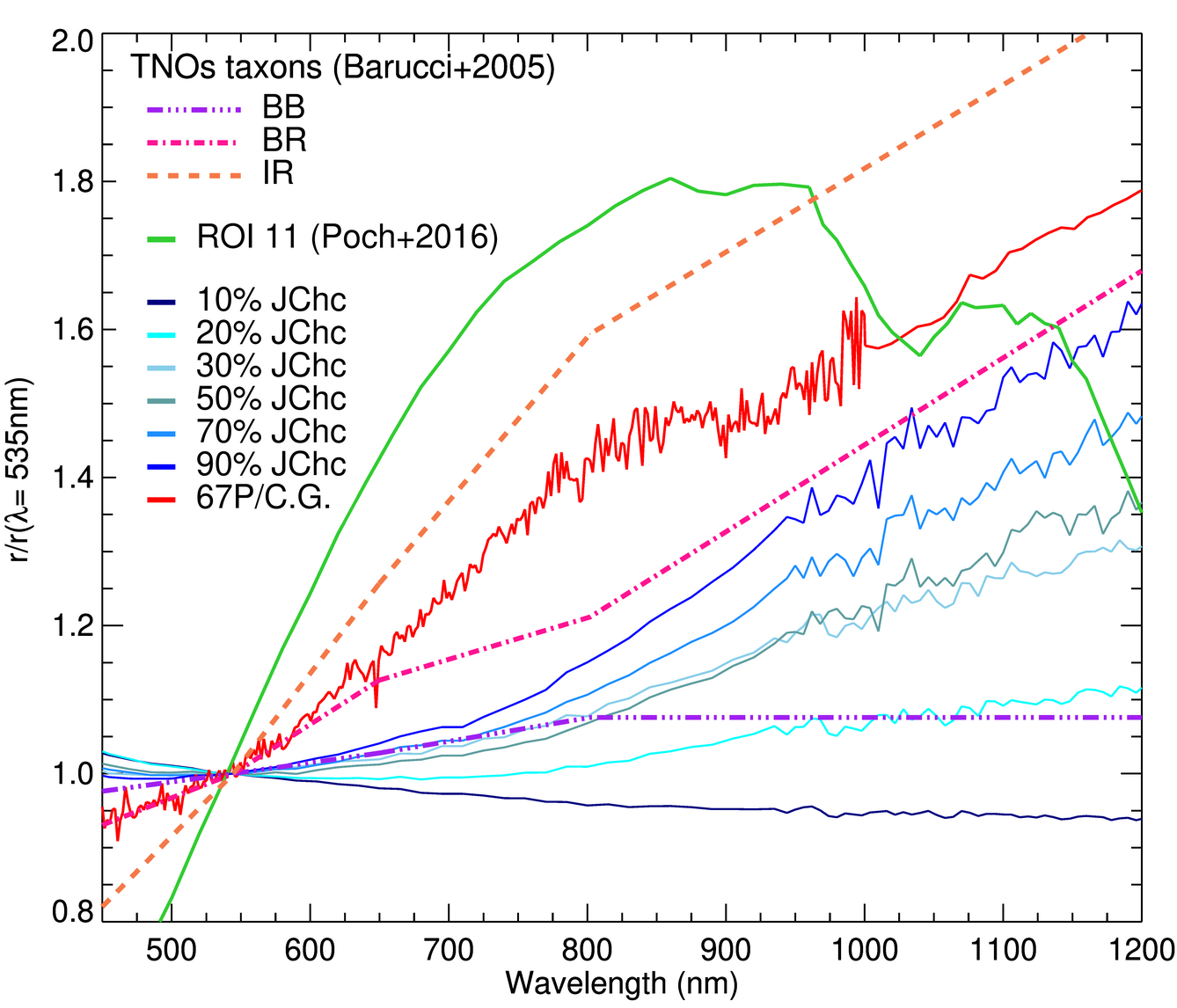
Figure 7: Comparison of the CoPhyLab mixtures’ spectra with that of 67P/CG and the normalised reflectances associated with the colors of the TNOs taxons discussed in Barucci et al. (2005). Although all spectra were photometricaly corrected, it should be noted that the CoPhyLab spectra were acquired at $\sim$ 0${}^{\circ}~{}$of incidence and phase angles, while the area, from which the spectrum from 67P/CG’s “body” was measured, was observed under $\sim$57$\pm$3${}^{\circ}~{}$of incidence, $\sim$86$\pm$2${}^{\circ}~{}$of emergence and $\sim$ 28.94$\pm$0.05${}^{\circ}~{}$of phase angle. The 1-$\sigma$ error-bars are omitted for clarity.

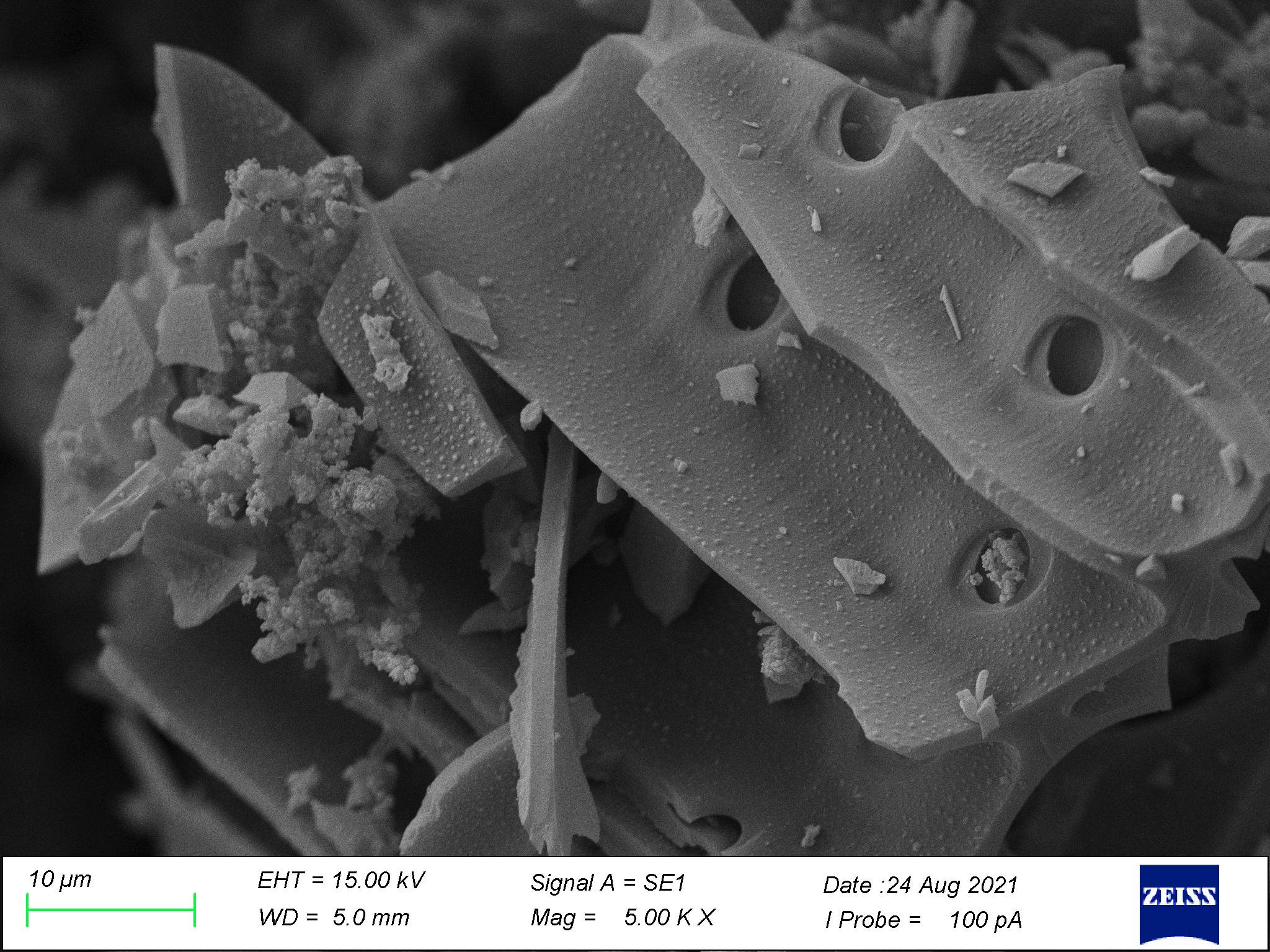
Figure 10: Zoom-in on the Cophylab mixture with 20% juniper charcoal, exhibiting small aggregates of SiO₂ particles sticking to the remnant of a juniper wood vessel structure. Micrometre-sized vessel wall pores and lignin protuberances hundreds of nanometres in sized are also clearly distinguishable in this image.

The TNOs taxons, labeled in Fig. 7 as BB, BR, and IR, respectively refer to the TNOs with small or no colour changes (i.e. displaying a “blue” spectral behaviour) across the considered wavelength domain, those with a slight-to-moderate colour change (i.e. displaying a “blue-red” spectral behaviour), and those displaying moderate-to-strong colour changes (i.e. presenting an moderately “red“ spectral behaviour).
As discussed in Fornasier et al. (2015) and illustrated here in Fig. 7 with the 67P/C-G spectrum from Filacchione et al. (2016), the normalised reflectance of 67P/CG’s typical terrains remains in between the “blue-red” and “red” profiles, whereas the illustrated CoPhyLab mixtures exhibit a diversity of spectral behaviours ranging from “bluer” than the TNOs’ BB group, to a behaviour intermediate between the BB and BR groups. This relative diversity of spectral profiles underlines the difference previously noted for the 535-882 nm spectral slopes (see Table 4). Through their monotonically increasing and incurved profile, the spectra of the CoPhyLab mixtures are also distinctly different from spectra of the water-ice/red tholins/activated charcoal intimate mixtures considered in Poch et al. (2016), which exhibited conspicuously higher spectral slopes across the visible range (see Fig. 7 and Feller et al. 2016), or from the PSOC-1532/pyrrhotite/dunite intimate mixture of sub-micron grains investigated by Rousseau et al. (2017) (see Fig. 10 of that paper), which also displayed visible spectral slopes larger than that of 67P/CG yet combined with an almost flat spectrum across the NIR domain.

Furthering the comparison to other small bodies beyond the main-belt, the color indices of the CoPhyLab mixtures were computed using standard BVRI filter profiles (Bessell, 1990) and then plotted against the colors indices of comets, Centaurs and Trojans, as well as TNOs collected and presented in Hainaut et al. (2012) and Peixinho et al. (2015). The authors of these studies gathered the (B-V), (V-I) and (V-R) indices for each of 24 comets, 144 Centaurs and Trojans, as well as 195 TNOs. The convex hulls for each group of objects are plotted in Fig. 8, alongside the colours indices of each TNO taxon defined in Barucci et al. (2005), and plotted here for reference, and those available for comets visited by spacecrafts (see Table 4).

As illustrated in Fig. 8, although the B-V and V-I colour indices of the CoPhyLab mixtures place inside, or close to, the V-R/V-I and B-V/V-I projections of the comets group’s hull (with the exception of the 10% juniper Charcoal mixture), a closer look at the V-R/B-V projections reveals their actual positions with respect to the different groupings. Almost all CoPhyLab materials exhibit overall colour indices consistent with the Centaurs and Trojans grouping, with the exception of the 10% and 20% JChc mixtures, whose B-V and V-R indices place them just on the outside of the hull. Similarly, these two indices also set all the CoPhyLab mixtures containing between 30% and 70% of juniper charcoal by mass on the lower edge of the TNOs group’s hull. On the other hand, only the pure juniper Charcoal sample and the mixture containing 90% juniper Charcoal are firmly set within the TNOs’ hull, with their respective propagated errors encroaching the volume of colour indices of comets.
Lastly, only the pure sample of SiO₂ and the measured spectrum of the mixture with 80 wt. % juniper charcoal present colour indices consistent with the diversity of the colours indices specific to the comets’ group. In particular, the SiO₂’s B-V and V-R indices closely match those of 1P/Halley and 103P/Hartley 2. While the 80% charcoal mixture differs from the other samples by its colors indices, these values remain nevertheless within the volume defined by the colours indices and their error-bars of the other mixtures.

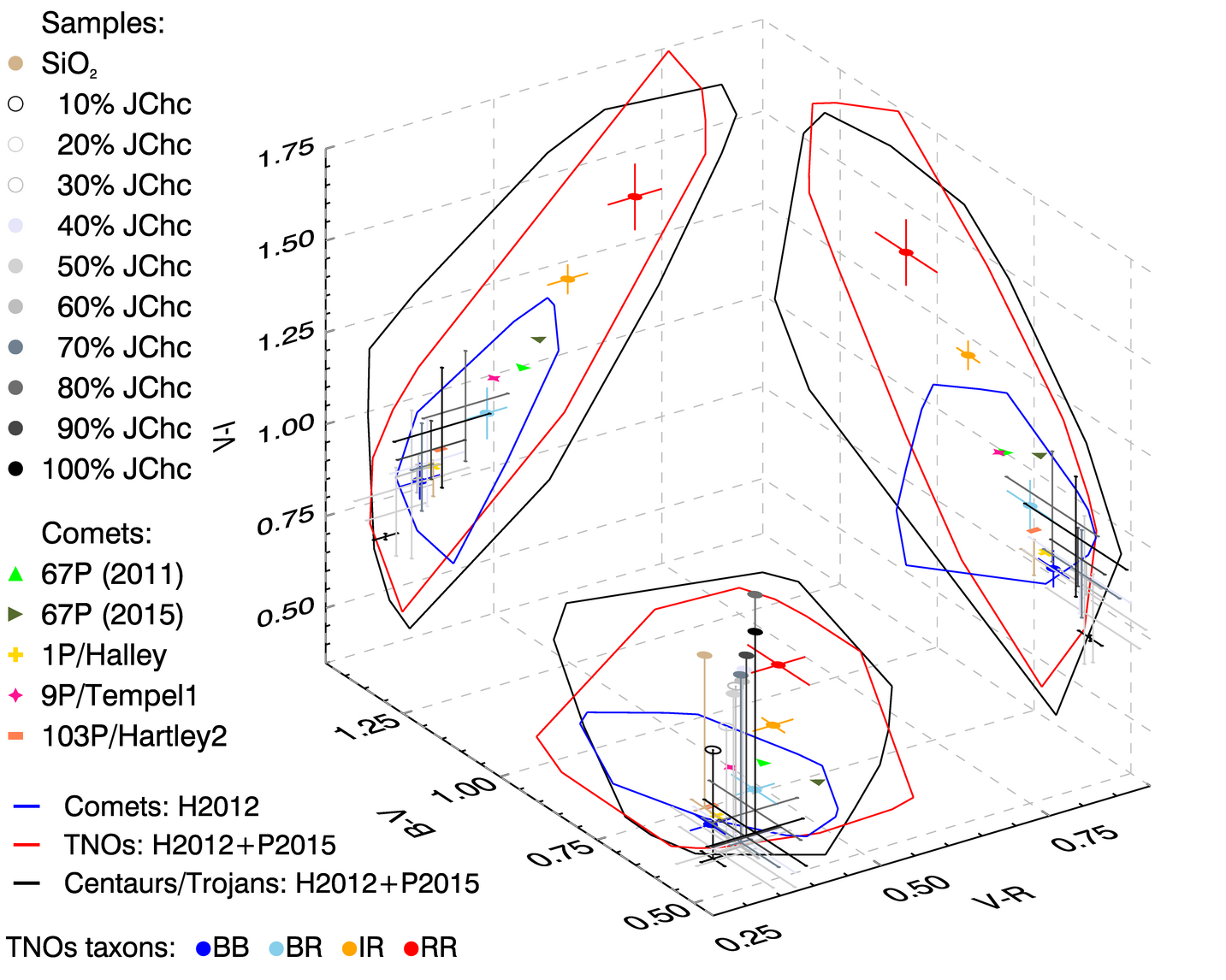
Figure 8: Diagram of the standard BVRI color differences for the CoPhyLab samples compared to those of comets visited by spacecrafts (see Table 4), and to other small bodies of the Outer Solar System. The area defined by the groups Comets, TNOs and Centaurs/Trojans were derived from the catalogues of Hainaut et al. (2012) (H2012) and Peixinho et al. (2015) (P2015), while the TNOs taxons correspond to those defined by Barucci et al. (2005).

5 Conclusions

In this paper, we have reported the first spectroscopic and photometric measurements for juniper charcoal and for intimate mixtures of juniper charcoal and silicon dioxide particles. Both series of measurements show that juniper charcoal, the dark fraction of the mixture, governs the overall spectro-photometric properties of the mixture.
While we find that the spectral behaviour of either end-members or mixtures do not provide a satisfactory match to an average spectrum of 67P/C-G’s dusty surfaces, the consideration of the spectral offset associated with the phase reddening phenomenon makes the visible spectral slopes of mixtures with more than 50 wt. % of juniper charcoal comparable to those of the average dusty surfaces on 67P/C-G’s nucleus. Comparison of the color-indices associated with the investigated material with those of small bodies of the Solar System shows that while some mixtures present color-indices consistent with values observed for comets, all the investigated materials fall more closely within the range of values expected for the bluest members of the TNOs as well as Centaurs and Trojans objects.

We also have shown that the photometric measurements of both juniper charcoal and silicon dioxide are best modeled as superficially porous and backscattering surfaces, presenting a more moderate opposition effect surge than the surfaces of 67P/C-G’s nucleus. These two materials most strongly differ through their single-scattering albedos. This albedo difference further transpires, for instance, when computing their respective geometrical albedos at 550 nm, with silicon dioxide having a geometric albedo about as bright as a 99 % reflectance calibration target, while that of the juniper charcoal would be, by that standard, about 25% lower than the geometrical albedo of the Imhotep/Ash border of the nucleus.
Furthermore, we have shown that the progression of the albedos of the intimate mixtures can be best fitted by a decreasing exponential law with respect to an increase in the juniper charcoal mass fraction, thus highlighting the strong influence of the more absorbent fraction over the overall reflectance properties of these intimate. The modeling of the variation of the mixtures’ single-scattering albedos at 550 nm, with respect to the juniper charcoal content, using a scale relation between the cross-sectional extinction efficiencies per unit length of the materials also supports this result. Moreover, collected SEM images show that the large distributions in scatterer-sizes for either material and the presence of large scale silicon dioxide aggregates are consistent with a Q^∗ ratio as large as 13.7$\pm$0.5.

We have thus found that intimate mixtures of juniper charcoal and silicon dioxide present some spectroscopic and photometric properties that are consistent with those of certain small bodies of the Solar System, such as TNOs and Centaurs, and some of these properties are close to, or of the same order as those found for the surface of 67P/Churyumov-Gerasimenko’s nucleus. While certain results presented in this study could warrant further investigations in the frame of the future experiments, either to further the physical likeness of the mixture to some of the observed dust- or pebble-covered surfaces of 67P/Churyumov-Gerasimenko or to investigate its physical properties at the micrometre and sub-micron scale, these mixtures will be considered in the upcoming sublimation experiments performed with the large CoPhyLab simulation chamber.

Data Availability

All spectroscopic and photometric data acquired for this study are available on the SSHADE database (10.26302/SSHADE/CF-1 and 10.26302/SSHADE/CF-2). In addition, the entire set of data and characterizations including the SEM images of the investigated samples will be made available on the Zenodo plateform (10.5281/zenodo.10280355) upon publication.

Appendix A Supplementary material

A.1 juniper charcoal particle-size range

A.2 Remnant of organic structures within the juniper charcoal

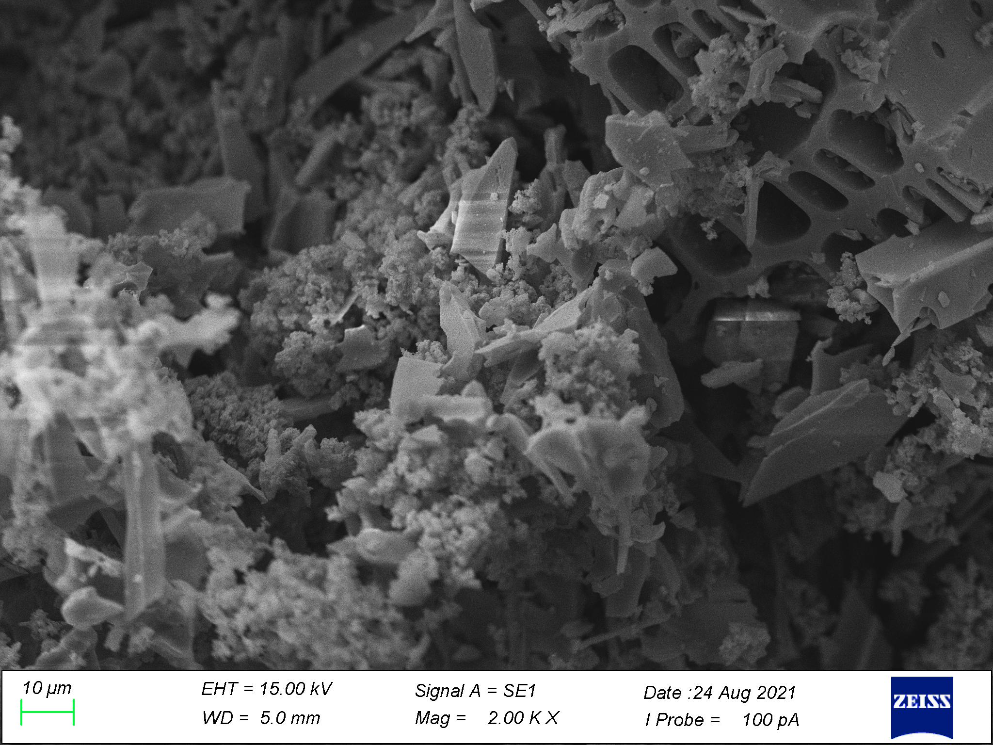
Figure 11: Zoom-in on the Cophylab mixture with 20% juniper charcoal, illustrating the tangle of SiO₂ grains and juniper charcoal fragments. In the background, a large remnant of juniper wood structure is also visible, which exhibits contiguous micrometre-sized cavities, which are consistent with fibre lumens.

Figure 12: Panel of SEM images for the CoPhylab mixtures with 10%, 30%, 50%, 70%, and 90% of juniper charcoal by mass. Zoom-in of the areas under the red squares are displayed in the SEM images of the right column.
These SEM images notably highlight micro-scale compositional heterogeneities, and reveal the presence of micrometre-sized SiO₂ agglomerates for any amount of juniper charcoal, as discussed in the main text.

A.3 Pictures of the samples

Figure 13: Pictures of the investigated samples taken under the same conditions. These pictures were acquired with a Nikon D5100 camera (f/5.6, 1/50 sec, 55mm of focal, ISO 100) under an emergence angle of $\sim$ 30${}^{\circ}~{}$and a main light source (a white neon) placed 2 metres right above the sample holder.

A.4 Plots of the samples’ phase curves and quality-fits

Figure 14: Phase curves of the investigated samples overplotted with the curves of the average best-fitting solutions and associated quality-fits.
In each case, the curve associated the HHS parameters listed in Table 3 appropriately the measured reflectance values of either end-members and all the considered mixtures.

References

- A’ Hearn et al. (2011) A’ Hearn M. F., et al., 2011, Science, 332, 1396
- Acton et al. (2018) Acton C., Bachman N., Semenov B., Wright E., 2018, Planet. Space Sci., 150, 9
- Altwegg et al. (2019) Altwegg K., Balsiger H., Fuselier S. A., 2019, ARA&A, 57, 113
- Andrés & Bona (2005) Andrés J., Bona M., 2005, Analytica Chimica Acta, 535, 123
- Bardyn et al. (2017) Bardyn A., et al., 2017, MNRAS, 469, S712
- Barucci et al. (2005) Barucci M. A., Belskaya I. N., Fulchignoni M., Birlan M., 2005, AJ, 130, 1291
- Barucci et al. (2016) Barucci M. A., et al., 2016, A&A, 595, A102
- Bertini et al. (2007) Bertini I., Thomas N., Barbieri C., 2007, A&A, 461, 351
- Bessell (1990) Bessell M. S., 1990, PASP, 102, 1181
- Bockelée-Morvan et al. (2017) Bockelée-Morvan D., et al., 2017, MNRAS, 469, S443
- Bohren & Huffman (1983) Bohren C. F., Huffman D. R., 1983, Absorption and scattering of light by small particles. John Wiley & Sons, Ltd, doi:https://doi.org/10.1002/9783527618156
- Brocksiepe (2000) Brocksiepe H.-G., 2000, Charcoal. American Cancer Society, doi:10.1002/14356007.a06_157
- Brownlee et al. (2012) Brownlee D., Joswiak D., Matrajt G., 2012, Meteoritics & Planetary Science, 47, 453
- Capaccioni et al. (2015) Capaccioni F., et al., 2015, Science, 347, aaa0628
- Ciarniello et al. (2015) Ciarniello M., et al., 2015, A&A, 583, A31
- Ciarniello et al. (2016) Ciarniello M., et al., 2016, MNRAS, 462, S443
- Ciarniello et al. (2020) Ciarniello M., et al., 2020, A&A, 634, A39
- Clark & Lucey (1984) Clark R. N., Lucey P. G., 1984, J. Geophys. Res., 89, 6341
- Cloutis et al. (1994) Cloutis E. A., Gaffey M. J., Moslow T. F., 1994, Icarus, 107, 276
- Cloutis et al. (2015) Cloutis E. A., et al., 2015, Icarus, 252, 39
- Davidsson et al. (2016) Davidsson B. J. R., et al., 2016, A&A, 592, A63
- De Sanctis et al. (2015) De Sanctis M. C., et al., 2015, Nature, 528, 241
- Delsanti et al. (2001) Delsanti A. C., Boehnhardt H., Barrera L., Meech K. J., Sekiguchi T., Hainaut O. R., 2001, A&A, 380, 347
- Dias et al. (2016) Dias A. F. J., Pirola L. P., Takeshita S., Lana A. Q., Brito J. O., Machado de Andrade A., 2016, Cerne, 22, 423
- Drozdovskaya et al. (2019) Drozdovskaya M. N., van Dishoeck E. F., Rubin M., Jørgensen J. K., Altwegg K., 2019, MNRAS, 490, 50
- El-Maarry et al. (2015) El-Maarry M. R., et al., 2015, A&A, 583, A26
- Elliott & Newns (1971) Elliott C. R., Newns G. R., 1971, Appl. Spectrosc., 25, 378
- Feller et al. (2016) Feller C., et al., 2016, MNRAS, 462, S287
- Feller et al. (2019) Feller C., et al., 2019, A&A, 630, A9
- Ferrari et al. (2018) Ferrari S., et al., 2018, MNRAS, 479, 1555
- Filacchione et al. (2016) Filacchione G., et al., 2016, Icarus, 274, 334
- Forest Products Laboratory (1980) Forest Products Laboratory 1980, Technical Report FPL-RN-04, Structure of Wood. USDA, Forest Service
- Fornasier et al. (2015) Fornasier S., et al., 2015, A&A, 583, A30
- Fornasier et al. (2016) Fornasier S., et al., 2016, Science, 354, 1566
- Fornasier et al. (2019) Fornasier S., et al., 2019, A&A, 630, A7
- Fornasier et al. (2020) Fornasier S., et al., 2020, A&A, 644, A142
- Gehrels et al. (1964) Gehrels T., Coffeen T., Owings D., 1964, AJ, 69
- Gladman et al. (2008) Gladman B., Marsden B. G., Vanlaerhoven C., 2008, Nomenclature in the Outer Solar System. The University of Arizona Press, pp 43–57
- Grynko & Shkuratov (2008) Grynko Y., Shkuratov Y. G., 2008, Light scattering from particulate surfaces in geometrical optics approximation. Springer Berlin Heidelberg, Berlin, Heidelberg, pp 329–382, doi:10.1007/978-3-540-48546-9_9, https://doi.org/10.1007/978-3-540-48546-9_9
- Grynko et al. (2018) Grynko Y., Shkuratov Y., Förstner J., 2018, Optics letters, 43(15), 3562–3565.
- Hainaut et al. (2012) Hainaut O. R., Boehnhardt H., Protopapa S., 2012, A&A, 546, A115
- Hänni et al. (2022) Hänni N., Altwegg K., Combi M., Fuselier S. A., De Keyser J., Rubin M., Wampfler S. F., 2022, Nature Communications, 13, 3639
- Hapke (1984) Hapke B., 1984, Icarus, 59, 41
- Hapke (1986) Hapke B., 1986, Icarus, 67, 264
- Hapke (1993) Hapke B., 1993, Theory of reflectance and emittance spectroscopy, 2 edn. Cambridge University Press
- Hapke (2002) Hapke B., 2002, Icarus, 157, 523
- Hapke (2008) Hapke B., 2008, Icarus, 195, 918
- Hasselmann et al. (2016) Hasselmann P. H., Barucci M. A., Fornasier S., Leyrat C., Carvano J. M., Lazzaro D., Sierks H., 2016, Icarus, 267, 135
- Hasselmann et al. (2017) Hasselmann P. H., et al., 2017, MNRAS, 469, S550
- Helfenstein & Shepard (2011) Helfenstein P., Shepard M. K., 2011, Icarus, 215, 83
- Helfenstein & Veverka (1989) Helfenstein P., Veverka J., 1989, in Binzel R. P., Gehrels T., Matthews M. S., eds, Asteroids II. pp 557–593
- Helfenstein et al. (1994) Helfenstein P., et al., 1994, Icarus, 107, 37
- Hoang et al. (2020) Hoang H. V., Fornasier S., Quirico E., Hasselmann P. H., Barucci M. A., Sierks H., Tubiana C., Güttler C., 2020, MNRAS, 498, 1221
- Izawa et al. (2014) Izawa M. R. M., Applin D. M., Norman L., Cloutis E. A., 2014, Icarus, 237, 159
- Jiang et al. (2018) Jiang Y., Lawrence M., Ansell M. P., Hussain A., 2018, The Royal Society Open Science, 5
- Jost et al. (2017a) Jost B., et al., 2017a, Planet. Space Sci., 145, 14
- Jost et al. (2017b) Jost B., Pommerol A., Poch O., Brouet Y., Fornasier S., Carrasco N., Szopa C., Thomas N., 2017b, Planet. Space Sci., 148, 1
- Kitamura et al. (2007) Kitamura R., Pilon L., Jonasz M., 2007, Appl. Opt., 46, 8118
- Kofman et al. (2015) Kofman W., et al., 2015, Science, 349
- Kothe et al. (2013) Kothe S., Blum J., Weidling R., Güttler C., 2013, Icarus, 225, 75
- Kreuzig et al. (2021) Kreuzig C., et al., 2021, Review of Scientific Instruments, 92, 115102
- Krüger et al. (2017) Krüger H., et al., 2017, A&A, 600, A56
- Labarre et al. (2017) Labarre S., Ferrari C., Jacquemoud S., 2017, Icarus, 290, 63
- Lamy et al. (2004) Lamy P. L., Toth I., Fernandez Y. R., Weaver H. A., 2004, The sizes, shapes, albedos, and colors of cometary nuclei. The University of Arizona Press, pp 223–264
- Lasue et al. (2011) Lasue J., Botet R., Levasseur-Regourd A. C., Hadamcik E., Kofman W., 2011, Icarus, 213, 369
- Lethuillier et al. (2022) Lethuillier A., et al., 2022, MNRAS, 515, 3420
- Li et al. (2004) Li J., A’Hearn M. F., McFadden L. A., 2004, Icarus, 172, 415
- Li et al. (2007) Li J.-Y., A’Hearn M. F., McFadden L. A., Belton M. J. S., 2007, Icarus, 188, 195
- Li et al. (2013) Li J.-Y., A’Hearn M. F., Belton M. J. S., Farnham T. L., Klaasen K. P., Sunshine J. M., Thomas P. C., Veverka J., 2013, Icarus, 222, 467
- Lipp (1992) Lipp E. D., 1992, Applied Spectroscopy Reviews, 27, 385
- Mannel et al. (2019) Mannel T., et al., 2019, A&A, 630, A26
- Maquet (2015) Maquet L., 2015, A&A, 579, A78
- Markkanen et al. (2018) Markkanen J., Agarwal J., Väisänen T., Penttilä A., Muinonen K., 2018, ApJ, 868, L16
- Marschall et al. (2020) Marschall R., Markkanen J., Gerig S.-B., Pinzón-Rodríguez O., Thomas N., Wu J.-S., 2020, Frontiers in Physics, 8, 227
- Masoumzadeh et al. (2016) Masoumzadeh N., et al., 2016, in 50th ESLAB Symposium: “From Giotto to Rosetta”.
- Moroz et al. (1998a) Moroz L. V., Arnold G., Korochantsev A. V., Wäsch R., 1998a, Icarus, 134, 253
- Moroz et al. (1998b) Moroz L. V., Arnold G., Korochantsev A. V., Wäsch R., 1998b, Icarus, 134, 253
- Muench et al. (1986) Muench R. E., Sagdeev R. Z., Jordan J. F., 1986, Nature, 321, 318
- Mustard & Hays (1997) Mustard J. F., Hays J. E., 1997, Icarus, 125, 145
- Oehler & Neukum (1991) Oehler A., Neukum G., 1991, Geophys. Res. Lett., 18, 253
- Oklay et al. (2016) Oklay N., et al., 2016, A&A, 586, A80
- Pajola et al. (2016) Pajola M., et al., 2016, A&A, 592, A69
- Peixinho et al. (2015) Peixinho N., Delsanti A., Doressoundiram A., 2015, A&A, 577, A35
- Petrov et al. (2012) Petrov D., Shkuratov Y., Videen G., 2012, J. Quant. Spectrosc. Radiative Transfer, 113, 2406
- Pilorget et al. (2013) Pilorget C., Vincendon M., Poulet F., 2013, Journal of Geophysical Research (Planets), 118, 2488
- Poch et al. (2016) Poch O., Pommerol A., Jost B., Carrasco N., Szopa C., Thomas N., 2016, Icarus, 267, 154
- Pommerol & Schmitt (2008) Pommerol A., Schmitt B., 2008, Journal of Geophysical Research: Planets, 113
- Pommerol et al. (2011) Pommerol A., Thomas N., Affolter M., Portyankina G., Jost B., Seiferlin K., Aye K.-M., 2011, Planetary Space Science, 59, 1601
- Pommerol et al. (2015) Pommerol A., Jost B., Poch O., El-Maarry M. R., Vuitel B., Thomas N., 2015, Planet. Space Sci., 109, 106
- Pommerol et al. (2019) Pommerol A., et al., 2019, Space Sci. Rev., 215, 37
- Preusker et al. (2017) Preusker F., et al., 2017, A&A, 607, L1
- Quirico et al. (2016) Quirico E., et al., 2016, Icarus, 272, 32
- Rahman et al. (2008) Rahman I., Vejayakumaran P., Sipaut C., Ismail J., Chee C., 2008, Ceramics International, 34, 2059
- Raponi et al. (2016) Raponi A., et al., 2016, MNRAS, 462, S476
- Rousseau et al. (2017) Rousseau B., et al., 2017, Icarus
- Rubin et al. (2019) Rubin M., et al., 2019, MNRAS, 489, 594
- Sanchez et al. (2012) Sanchez J. A., Reddy V., Nathues A., Cloutis E. A., Mann P., Hiesinger H., 2012, Icarus, 220, 36
- Sandford et al. (2021) Sandford S. A., Brownlee D. E., Zolensky M. E., 2021, Chapter 4 - The Stardust sample return mission. Elsevier, pp 79–104, doi:10.1016/B978-0-12-818330-4.00004-5, https://www.sciencedirect.com/science/article/pii/B9780128183304000045
- Schröder et al. (2014) Schröder S. E., Grynko Y., Pommerol A., Keller H. U., Thomas N., Roush T. L., 2014, Icarus, 239, 201
- Seeliger (1887) Seeliger H., 1887, Zur Theorie. der Beleuchtung der grossen Planeten insbesondere des Saturn. Imperial Acamedy of Natural Sciences of Bayern
- Shepard & Helfenstein (2007) Shepard M. K., Helfenstein P., 2007, Journal of Geophysical Research (Planets), 112, E03001
- Shevchenko et al. (2012) Shevchenko V. G., et al., 2012, Icarus, 217, 202
- Shkuratov et al. (2012) Shkuratov Y., Kaydash V., Korokhin V., Velikodsky Y., Petrov D., Zubko E., Stankevich D., Videen G., 2012, J. Quant. Spectrosc. Radiative Transfer, 113, 2431
- Simonelli et al. (1996) Simonelli D. P., Veverka J., Thomas P. C., Helfenstein P., Carcich B. T., Belton M. J., 1996, Icarus, 120, 38
- Simonelli et al. (1998) Simonelli D. P., Wisz M., Switala A., Adinolfi D., Veverka J., Thomas P. C., Helfenstein P., 1998, Icarus, 131, 52
- Stephens & Gustafson (1991) Stephens J. R., Gustafson B. A. S., 1991, Icarus, 94, 209
- Svarovskly (1987) Svarovskly L., 1987, Powder Testing Guide, 1 edn. Springer Dordrecht, https://link.springer.com/book/9781851661374
- Taylor et al. (2017) Taylor M. G. G. T., Altobelli N., Buratti B. J., Choukroun M., 2017, Philosophical Transactions of the Royal Society of London Series A, 375, 20160262
- Thomas & Keller (1989) Thomas N., Keller H. U., 1989, A&A, 213, 487
- Thomas et al. (1996) Thomas P. C., Adinolfi D., Helfenstein P., Simonelli D., Veverka J., 1996, Icarus, 123, 536
- Tubiana et al. (2008) Tubiana C., Barrera L., Drahus M., Boehnhardt H., 2008, A&A, 490, 377
- Tubiana et al. (2011) Tubiana C., Böhnhardt H., Agarwal J., Drahus M., Barrera L., Ortiz J. L., 2011, A&A, 527, A113
- Tubiana et al. (2015) Tubiana C., et al., 2015, A&A, 583, A46
- Warren & Wiscombe (1980) Warren S. G., Wiscombe W. J., 1980, Journal of Atmospheric Sciences, 37, 2734
- Workman & Weyer (2012) Workman J. J., Weyer L., 2012, Practical Guide and Spectral Atlas for Interpretive Near-Infrared Spectroscopy. CRC Press, doi:10.1201/b11894
- Yoldi et al. (2015) Yoldi Z., Pommerol A., Jost B., Poch O., Gouman J., Thomas N., 2015, Geophys. Res. Lett., 42, 6205
- Zerull (1976) Zerull R. H., 1976, Beitraege zur Physik der Atmosphaere, 49, 168
- Zhuravlev (2000) Zhuravlev L., 2000, Colloids and Surfaces A: Physicochemical and Engineering Aspects, 173, 1