Two $T$-linear scattering rate regimes in the triangular lattice Hubbard model

Abstract

In recent years, the $T$-linear scattering rate found at low temperatures, defining the strange metal phase of cuprates, has been a subject of interest. Since a wide range of materials have a scattering rate that obeys the equation $\hbar/\tau\approx k_{B}T$, the idea of a universal Planckian limit on the scattering rate has been proposed. However, there is no consensus on proposed theories yet. In this work, we present our results for the $T$-linear scattering rate in the triangular lattice Hubbard model obtained using the dynamical cluster approximation. We find two regions with $T$-linear scattering rate in the $T$—$p$ phase diagram: one emerges from the pseudogap to correlated Fermi liquid phase transition at low doping, whereas the other is solely caused by large interaction strength at large doping.

I Introduction

At the lowest temperatures in any metal, when the phonon contribution becomes negligible, one expects a Fermi liquid with $T^{2}$ resitivity. Although it is indeed the case in most materials, many do not abide by this rule, having instead a linear in temperature scattering rate. This is the case for a wide variety of materials, such as twisted bilayer graphene  [1, 2, 3], transition metal dichalcogenides [4], pnictides superconductors [5], heavy fermions [6, 7, 8], organic superconductors [5] and cuprates [9, 10, 11]. This kind of behavior is even found theoretically in the square lattice Hubbard model [12] and in the Sachdev–Ye–Kitaev model [13].

$T$-linear scattering rate is often the result of electron-phonon scattering. This is the case for example in copper and twisted bilayer graphene [14]. However, at temperatures lower than the Debye temperature, this mechanism can no longer explain $T$-linear scattering. $T$-linear scattering rate must then be caused by another type of interaction. Metals that exhibit $T$-linear scattering rate at high temperature, beyond the Mott-Ioffe-Regel limit $k_{F}\ell\sim 1$, are called bad metals [15, 16, 17]. When the linear regime extends asymptotically close to $T=0$, we refer to strange metal behavior. Cuprates are a nice case study of strange metals since their scattering rate has been thoroughly studied from the day of their discovery [18, 19]. In addition, their $T$-linear scattering rate spans a large portion of the cuprate’s phase diagram, sometimes up to high temperatures [19, 18].

The idea of a universal limit on scattering rate was presented to explain the $T$-linear scattering rate [20]. Using Drude’s formula to find the relaxation time $\tau$, it has been observed that many strange metals obey the simple equation $\frac{\hbar}{\tau}=\alpha k_{B}T$, where $\alpha$ is between 0.7 and 1.1 [21, 22, 23]. The idea that this universal law could also be applied to very different materials with very similar value of $\alpha$ has led some to believe that electrons are subject to a universal Planckian limit of $\alpha\sim 1$ [24, 10, 25, 26, 27, 28, 29].

The close proximity of strange-metal behavior to optimal doping in cuprates has led some to believe that understanding it could be the key to uncovering the mechanism behind superconductivity in hole-doped cuprates [30, 31]. The $T$-linear dependence of the scattering rate in cuprates is still a subject of research [32, 33, 34, 35].

In this work, we present the phase diagram and the temperature-dependent scattering rate on the hole-doped triangular-lattice Hubbard model using the dynamical cluster approximation (DCA) [36] for the six-site cluster shown on Fig. 1a). DCA is a cluster extension of dynamical mean-field theory (DMFT) that is particularly suited for doped Mott insulators in regimes where long-wavelength particle-particle and particle-hole fluctuations are negligible. The geometrical frustration inherent to the triangular lattice is particularly useful to suppress the above-mentioned fluctuations, making the thermodynamic limit reachable at finite temperature on small lattices. Our three main results are as follows:

First, our most unexpected finding is the observation of $T$-linear electron scattering in two distinct regions of the phase diagram: one at low dopings and another at higher dopings. We attribute the former to doped-Mott insulator physics, showing that $T$-linear scattering at low doping is linked to the metal-to-pseudogap first-order transition known as the Sordi transition [37, 38, 39]. We refer to this regime as the Mott-driven $T$-linear scattering rate. Conversely, at higher dopings, we propose that the $T$-linear scattering is solely governed by strong interactions, occurring very far from the Mott transition. We refer to this region as the interaction-driven $T$-linear scattering rate. It is noteworthy that in both cases, we noted in Tab. 1 which characteristics usually pertaining to strange metals they respect.

Second, the role of long-wavelength magnetic fluctuations is not important in either regimes since, at the temperatures that we can reach, frustration on the triangular lattice limits their effect. Indeed, for values of $U$ that we explore, close to the Mott transition, it has been found that even at half-filling magnetic order is not apparent [40, 41, 42, 43, 44, 45, 46].

Third, we find that even on the triangular lattice, the quasiparticle scattering rate of the interaction-driven $T$-linear scattering rate is very near the Planckian limit ($\alpha\sim 1$).

Although our work may be related to the fundamental physics that drives the strange metal in cuprates, our model most likely represents what would be seen in doped $\kappa$-ET structured doped organic superconductors [47, 48], field-effect doped organic superconductors [49], silicon triangular lattice simulators [50] or cold atoms experiments [51, 52, 53]. Nevertheless, we find it valuable to draw comparisons with cuprates, given their extensive history of exploration.

In the following sections, we discuss the model, then uncover the phase diagrams that will drive our discussion over the two possible $T$-linear scattering rate mechanisms.

II Methodology

Here we present the model, then discuss the method that we use, and finally, comment on observables of interest.

II.1 Model.

We capture the complex interplay between kinetic energy and potential energy of electrons on a lattice with the one-band Hubbard model  [54, 55, 56, 57]. The Hamiltonian is given by

$$\mathcal{H}=-\sum_{i,j,\sigma}t_{ij}c_{i\sigma}^{\dagger}c_{j\sigma}+U\sum_{i}n_{i\uparrow}n_{i\downarrow}-\mu\sum_{i\sigma}n_{i\sigma},$$ (1)

where $c_{i\sigma}^{\dagger}$ and $c_{i\sigma}$ are respectively the creation and annihilation operators on site $i$ with spin $\sigma$, $n_{i\sigma}$ is the number operator, $t_{ij}$ is the kinetic energy associated to a hopping between sites $i$ and $j$, $U$ is the on-site Coulomb repulsion, and $\mu$ is the chemical potential. We work in natural units, thus interatomic distance $a$, Planck’s $\hbar$ and Boltzmann’s $k_{B}$ constants are unity, as is $t$ the nearest-neighbor hopping.

The lattice is shown on Fig. 1 a). We take $t=-t^{\prime}=1$ so that the lattice is triangular. The sign of $t^{\prime}$ would change electrons for holes. Here we focus mostly on hole doping. Another hopping $t^{\prime}$ crossing the one illustrated would transform this problem into the problem of cuprates. We will later discuss implications of our results for cuprates.

II.2 Solving the model.

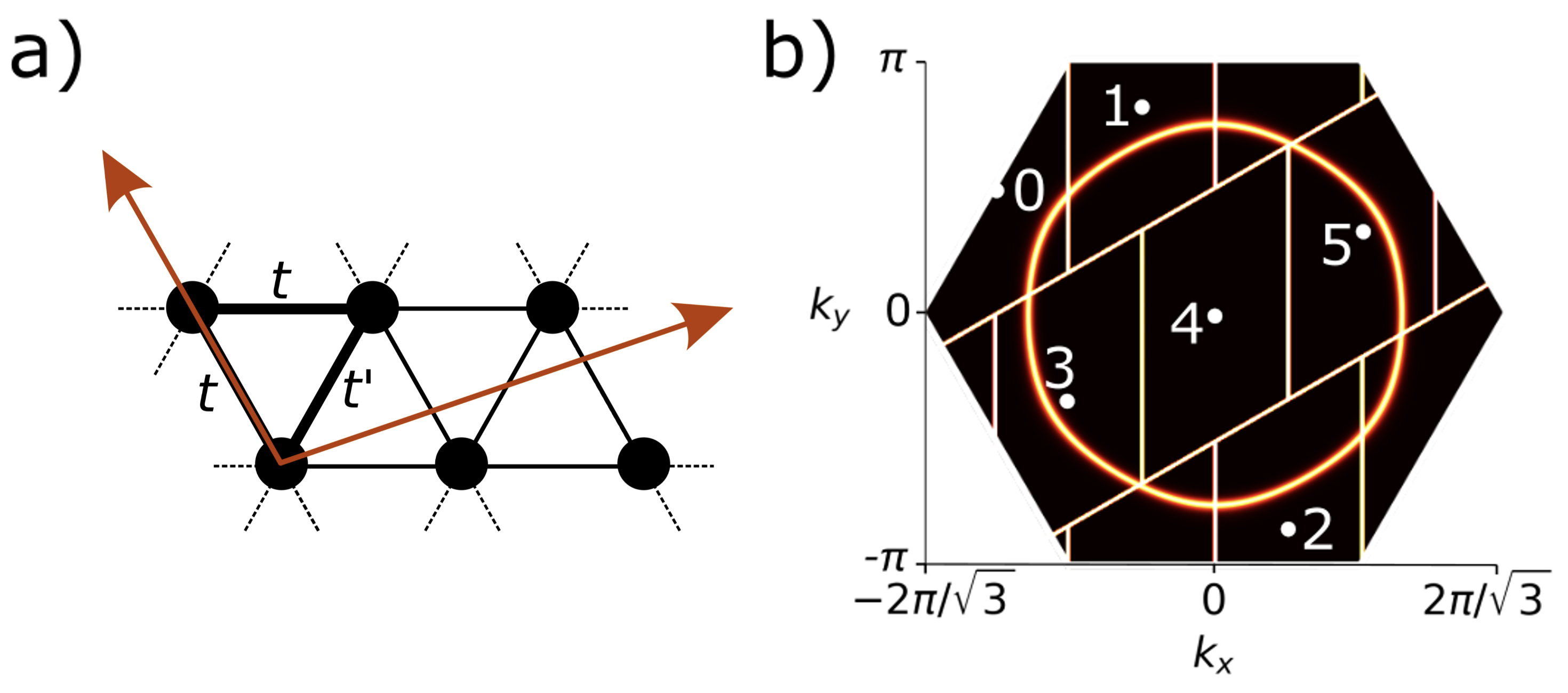
Figure 1: a) Hopping terms on the triangular lattice b) Fermi surface for $U=0$ and $n=1$ at $T=0.1$ in the triangular lattice. The different patches used in the Brillouin zone of the triangular lattice and on the proxy square lattice made of the reciprocal lattice-vectors are illustrated. The superlattice vectors in red illustrate the periodic boundary conditions. Although $t^{\prime}=-t$ is satisfied in our work, this connectivity corresponds to a bipartite lattice when $t^{\prime}=0$. The illustrated Fermi surface is a hole Fermi surface.

References 58, 59 have shown that in DCA, a six-site cluster impurity in a bath  [60, 36, 61, 62] describes the same complex physics as the larger 12-site cluster at temperatures that are reachable near the Mott transitions. This is discussed further in Appendix A. For this reason, we use the same six-site cluster as in Ref. 58, defined by the superlattice vectors $R_{x}=(3,1)$ and $R_{y}=(2,0)$ as shown on Fig. 1a). Periodic boundary conditions in DCA impose that the Brillouin zone be separated into patches, one for every site on the impurity, their shape being just another degree of freedom [63, 64]. Fig. 1b) presents the layout we use. To illustrate how the Fermi surface is distributed among the patches we chose, the non-interacting Fermi surface is also displayed.

In DCA, one starts with a guess for the free Green’s function

$$\mathcal{G}_{0,\sigma}(i\omega_{n},\textbf{K}_{i})=\frac{1}{i\omega_{n}-\bar{\epsilon}_{\textbf{K}_{i}}+\mu-\Delta_{\sigma}(i\omega_{n},\textbf{K}_{i})},$$ (2)

where we define $\bar{\epsilon}_{\textbf{K}_{i}}=\sum_{\tilde{\textbf{k}}}\epsilon_{\textbf{K}_{i}+\tilde{\textbf{k}}}$, with $\sum_{\tilde{\textbf{k}}}$ the sum on every $\mathbf{\tilde{k}}$ in a patch, $\epsilon_{\textbf{K}_{i}+\tilde{\textbf{k}}}=\epsilon_{\mathbf{k}}$ the bare band dispersion, $\omega_{n}$ the $n^{\text{th}}$ fermionic Matsubara frequency, defined as $\omega_{n}=\frac{(2n+1)\pi}{\beta}$, with $\beta$ the inverse of temperature. Finally, $\Delta_{\sigma}(i\omega_{n},\textbf{K}_{i})$ is the hybridization function, linking the bath and the impurities.

To find the cluster Green’s function $\mathcal{G}_{c,\sigma}(i\omega_{n},\textbf{K}_{i})$, one sends the non-interacting Green’s function to an impurity solver. Here we use the continuous-time auxiliary-field (CT-AUX)[65, 61] quantum Monte-Carlo impurity solver because it scales well with the cluster size. Using the Dyson equation, one can extract the cluster self-energy

$$\Sigma_{c,\sigma}(i\omega_{n},\textbf{K}_{i})=\mathcal{G}^{-1}_{0,\sigma}(i\omega_{n},\textbf{K}_{i})-\mathcal{G}^{-1}_{c,\sigma}(i\omega_{n},\textbf{K}_{i}).$$ (3)

Projecting the lattice Green’s function on the patches

$$\mathcal{G}_{loc,\sigma}(i\omega_{n},\textbf{K}_{i})=\sum_{\tilde{\textbf{k}}}\frac{1}{i\omega_{n}-{\epsilon}_{\textbf{K}_{i}+\tilde{\textbf{k}}}+\mu-\Sigma_{c,\sigma}(i\omega_{n},\textbf{K}_{i})},$$ (4)

leads to the self-consistency condition $\mathcal{G}_{loc,\sigma}(i\omega_{n},\textbf{K}_{i})=\mathcal{G}_{c,\sigma}(i\omega_{n},\textbf{K}_{i})$ from which the hybridization function necessary for the next iteration can be obtained:

$$\Delta_{\sigma}(i\omega_{n},\textbf{K}_{i})=i\omega_{n}-\mu-\mathcal{G}^{-1}_{loc,\sigma}(i\omega_{n},\textbf{K}_{i})-\Sigma_{c,\sigma}(i\omega_{n},\textbf{K}_{i}).$$ (5)

Substituting into the non-interacting Green’s function Eq. 2, the next iteration of the DCA calculation begins.

Since the Green’s function is symmetric in spin, we drop that index. We use the converged solution given by the data compilation algorithm proposed in Ref. 58. Since DCA is a coarse-grained method, the momentum dependence of observables $\mathcal{O}$ are averaged over patches. The Green’s function and the self-energy are constant within each patch $i$. Dividing out the Brillouin zone into six patches $\mathbf{K}_{i}$, the symmetries of the triangular lattice impose that $\mathcal{O}(\mathbf{K}_{1})=\mathcal{O}(\mathbf{K}_{2})$ and $\mathcal{O}(\mathbf{K}_{3})=\mathcal{O}(\mathbf{K}_{5})$. The patches are identified on Fig. 1b).

II.3 Observables.

One of he important observables that we consider is the local scattering rate $\Gamma=1/\tau$, where $\tau$ is the lifetime. This quantity is extracted from the local self-energy as

$$\Gamma=1/\tau=-\text{Im}\left(\sum_{i}^{N_{c}}\Sigma(\omega=0,\textbf{K}_{i})\right).$$ (6)

To obtain $\Sigma(\omega=0,\textbf{K}_{i})$, we perform the analytical continuation using a simple polynomial fit on the first three Matsubara frequencies of $\text{Im}\Sigma(i\omega_{n},\textbf{K}_{i})$, and extrapolate the polynomial to $\omega=0$. In Appendix B, we show how the results are affected by the choice of polynomial order. This kind of approximation does not give accurate results at high temperatures, but it improves at low temperatures where the Matsubara frequencies are closer. For this reason, we limit ourselves to $T$ lower than $0.2$. Also, due to the fermion sign problem and general low acceptance rate at low temperature, it is practically impossible to reach $T$ below $0.02$. For a typical value of hopping $t$ in the cuprates of 0.3 eV, the range of temperature achievable with DCA would then range approximately between 70K and 700K. In BEDT organics the corresponding scales would be ten times smaller.

Here, we mostly focus on the electron scattering rate given by Eq. 6 instead of the quasiparticle scattering rate that would be obtained by multiplying Eq. 6 by the quasiparticle renormalization factor $Z$. This is because, even if the density of states presents a quasiparticle peak, some suggest that the quasiparticle picture breaks down in the strange metal [66]. We find that the exponent $n$ for the temperature dependence of the scattering rate does not change significantly when comparing electron scattering rate with quasiparticle scattering rate. There is however a sizable change in the slope caused by $Z$.

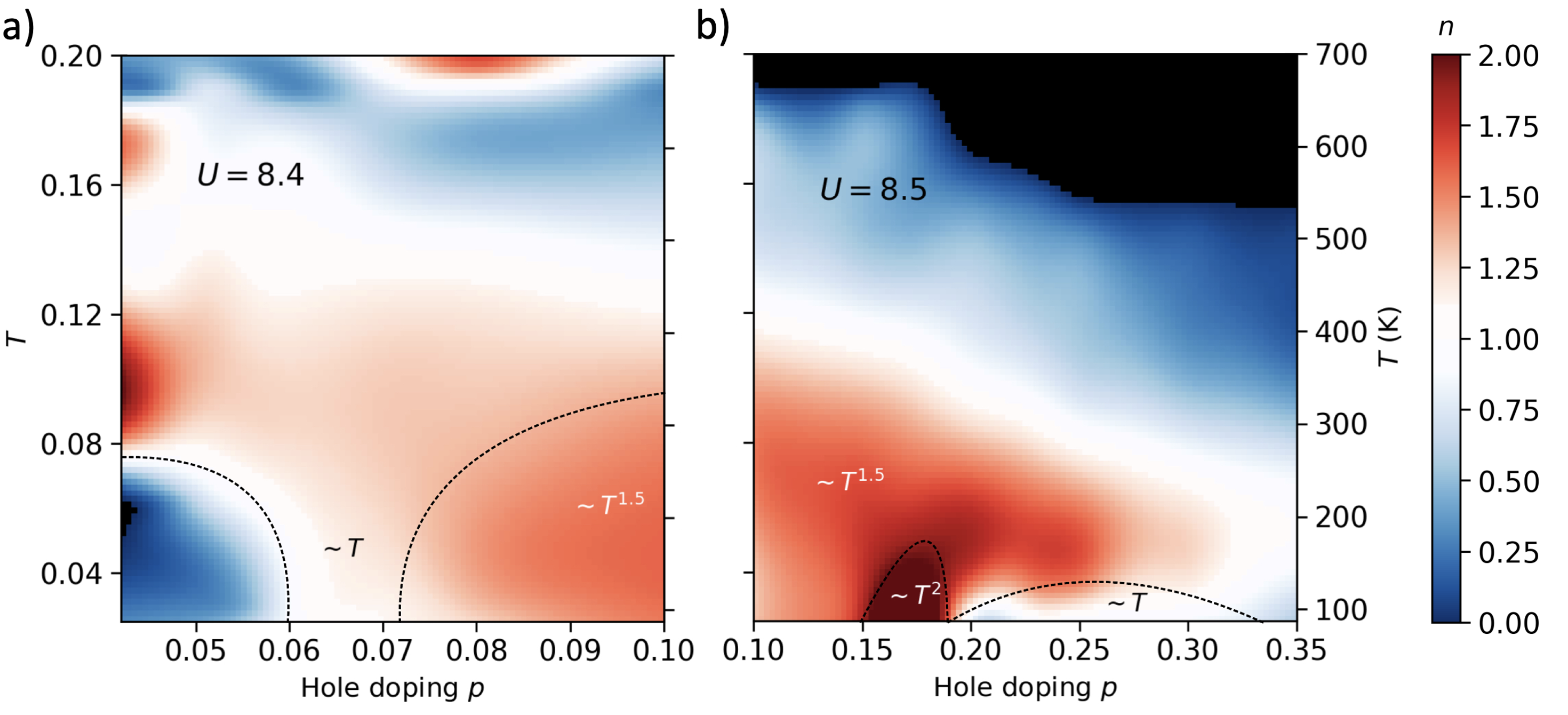
Figure 2: a) Temperature-doping phase diagram of the local scattering rate, defined by Eq. (6), for $U=8.4$. Color coding represents the value of $n$ obtained, as described in Appendix C, from a local fit of the form $1/\tau=\alpha T^{n}+b$ of the scattering rate. The dashed line between $p=0.04$ and $p=0.06$ represents the temperature where the scattering rate starts to fall rapidly with temperature, whereas the one between $p=0.07$ and $p=0.1$ delimits the region where the scattering rate is proportional to $T^{1.5}$. b) Corresponding data for $U=8.5$ in the high-doping range. The dashed line between $p=0.15$ and $p=0.18$ represents the temperature where we find a $T^{2}$ dependent scattering rate, whereas the one between $p=0.18$ and $p=0.34$ delimits the region where we find $T$-linear scattering rate at high dopings. This region of linearity between $p=0.18$ and $p=0.34$ appears very small on this figure because interpolation became difficult at lower temperature. Fig.5 shows that the data extends to $T=0.02$ and continues to exhibit linearity. The temperature scale is fixed by taking $t=0.3$eV, typical value for cuprates

III Results

We compute the scattering rate as a function of temperature for various hole-dopings of the Mott insulator. Doing this for many dopings, we build two temperature-doping phase diagrams  where we summarize the temperature dependence of $\Gamma=1/\tau$ by color-coding the local exponent $n$ obtained form a local fit of the form $1/\tau=\alpha T^{n}+b$ on the data, as described in Appendix C.

We choose values of interaction $U$ slightly higher the critical value of $U$ for the Mott transition at half-filling ($U\approx 8.2$ for $T=0.15$ [58]). The first diagram on Fig. 2a) obtained at $U=8.4$, focuses on the low doping behavior. The second, presented on Fig. 2b) for $U=8.5$, focuses on high dopings. At low dopings, the value of $U$ is chosen slightly smaller because lowering $U$ increases the average sign in the Monte-Carlo calculations and makes it possible to converge in the pseudogap regime at slightly lower temperatures. The scattering rates that we used to draw these phase diagrams as a function of temperature at $U=8.4$ and $U=8.5$ are displayed respectively on Figs. 3 and 5.

The results between 10% and 15% hole doping in Fig.  2b) exhibit a $T^{1.5}$ dependence of the scattering rate, qualitatively different from that found in organics [68, 47] or in cuprates [10, 22, 9, 24]. Nevertheless, both doping regions illustrated in Figs. 2a) and 2b) display $T$-linear scattering rate for different ranges of temperature. Indeed, we find $1/\tau\sim T$ in Fig. 2a) for a wide range of temperature for $p$ near $0.06$, while in Fig. 2b), we find $T$-linear scattering for hole dopings between $0.2$ and $0.3$, from $T\approx 0.03$ down to the lowest temperature achievable. This leads us to believe that two different mechanisms are responsible for the $T$-linear scattering rates.

In the following sections, we present the two different regimes of $T$-linear scattering rate. In the first section III.1, we show that the low-doping $T$-linear scattering rate is deeply rooted in the existence of the Sordi transition, the same pseudogap-metal first-order transition that is continuously connected to the Mott transition as reported in Ref. 38. We thus use the name Mott-driven $T$-linear scattering rate, even though superexchange also plays a role in the Sordi transition, as can be argued from the fact that single-site DMFT finds a direct insulator to metal transition with doping [69]. Then, in section III.2, we show that interactions seem to be the sole driver of the high doping $T$-linear scattering rate, thus the name interaction-driven $T$-linear scattering rate.

Both regimes of $T$-linear scattering rate found in this research share similarities with the strange metal phase found in cuprates. A list of these similarities can be found in table 1. However, since both regimes have $T$-linear scattering rates that extrapolate to negative values at $T=0$, we know that the $T$-linear scattering rate cannot be sustained at $T\to 0$. Because of this, we do not use the term strange metal to describe our findings. We instead use $T$-linear scattering rate.

	$1/\tau\sim T$	$1/\tau\sim T$ as $T\to 0$	$1/\tau\sim T$ as $T\to\infty$	$\omega/T$ scaling	Planckian dissipation	Extended range of doping	Isotropic scattering rate
Mott-driven ($p\approx 4\%\sim 6\%$)	✓	✗	✓	✓	✗	✓	✗
Interaction-driven ($p\approx 20\%\sim 30\%$)	✓	✗	✗	✗	✓	✓	✓

Table 1: Table summarizing the similarities and differences between the usual strange metal, whose properties appear on the top row, and the two $T$-linear scattering rate regimes in this paper, namely Mott-driven and interaction-driven.

III.1 Mott-Driven $T$-linear scattering rate

Fig. 2a) displays the first region where we find $T$-linear scattering, what we call the Mott-driven $T$-linear scattering rate. This region spans a large area of the phase diagram, and goes down to the lowest temperatures near $p=0.065$. A clearer picture emerges from Fig. 3, where we present the scattering rate as a function of temperature and doping for the first, second and third patches . At $p=0.06$, we see in Fig. 2a) and Fig. 3 that $T$-linear scattering rate ranges from the lowest achievable temperatures to around $T=0.2$. There is a slight deviation from the $T$-linear regime seen in Fig. 2a) for $T\approx 0.08$. The raw data for the scattering rate at $p=0.06$ in Fig. 3, shows that this deviation from the $T$-linearity is barely noticeable. A similar deviation from $T$-linear scattering is also found in LSCO [10]. Moreover, the scattering rate in this $T$-linear scattering rate region is not isotropic. Since our model does not include phonons, the $T$-linear scattering found at high temperature near $p=0.06$ is not a result of electron-phonon scattering at $T>T_{D}$.

From Fig. 2a) at $U=8.4$ and from the scattering rates on Fig. 3, one observes that the $T$-linear scattering rate at low temperature is only present for dopings near $p=0.06$. The deviation from linearity between $T=0.12$ and $T=0.18$ is very small. Dopings lower than $p=0.04$ are shown only in Fig. 3. There one finds an upturn in the scattering rate. This upturn in characteristic of the pseudogap phase. On the other hand, when $p$ increases, we find, at low-$T$, a $T^{1.5}$ scattering rate. Since the low-doping $T$-linear scattering rate occurs at low temperature only for a very specific doping, it is likely to arise from a quantum-critical point. For $U=8.4$, this quantum-critical point would be located near $p^{*}=0.06$.

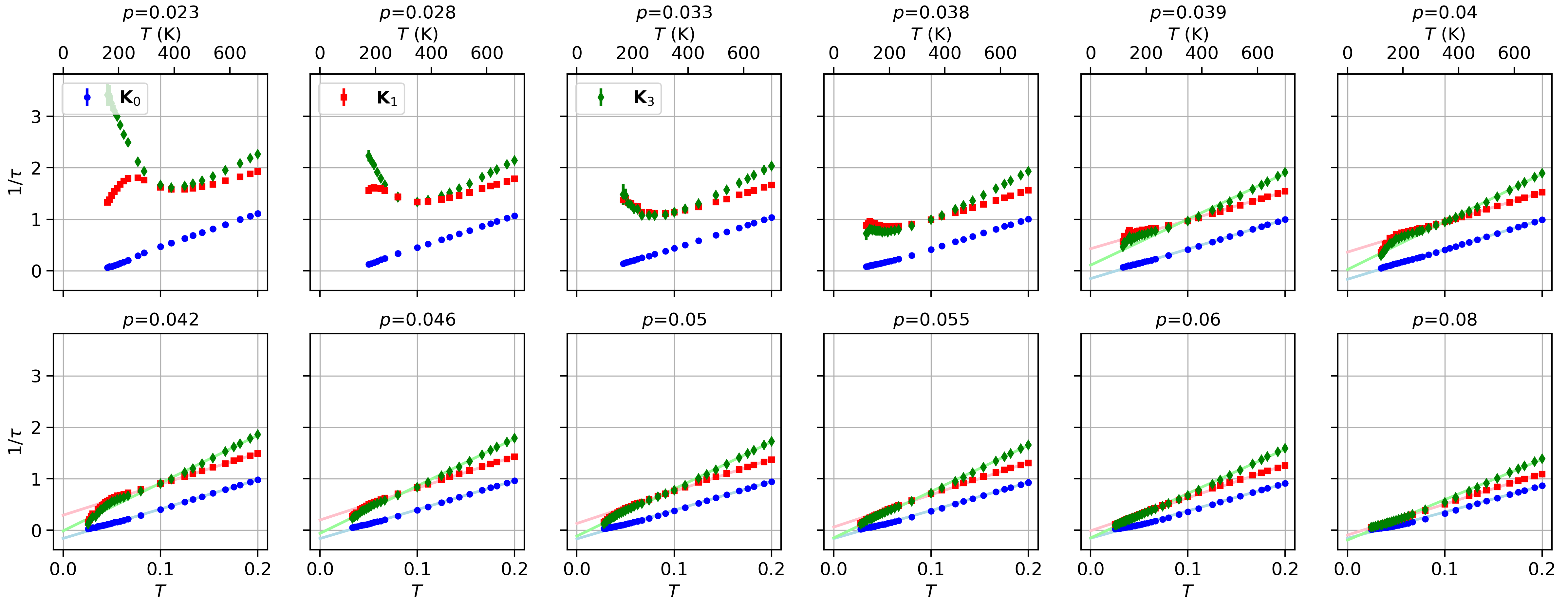
Figure 3: Scattering rate as a function of temperature for hole dopings between $p=0.023$ and $p=0.08$ at $U=8.4$ for the zeroth, first and third patches of the triangular lattice in Fig. 1b). The temperature scale is fixed by taking $t=0.3$eV, typical of the numbers for cuprates.

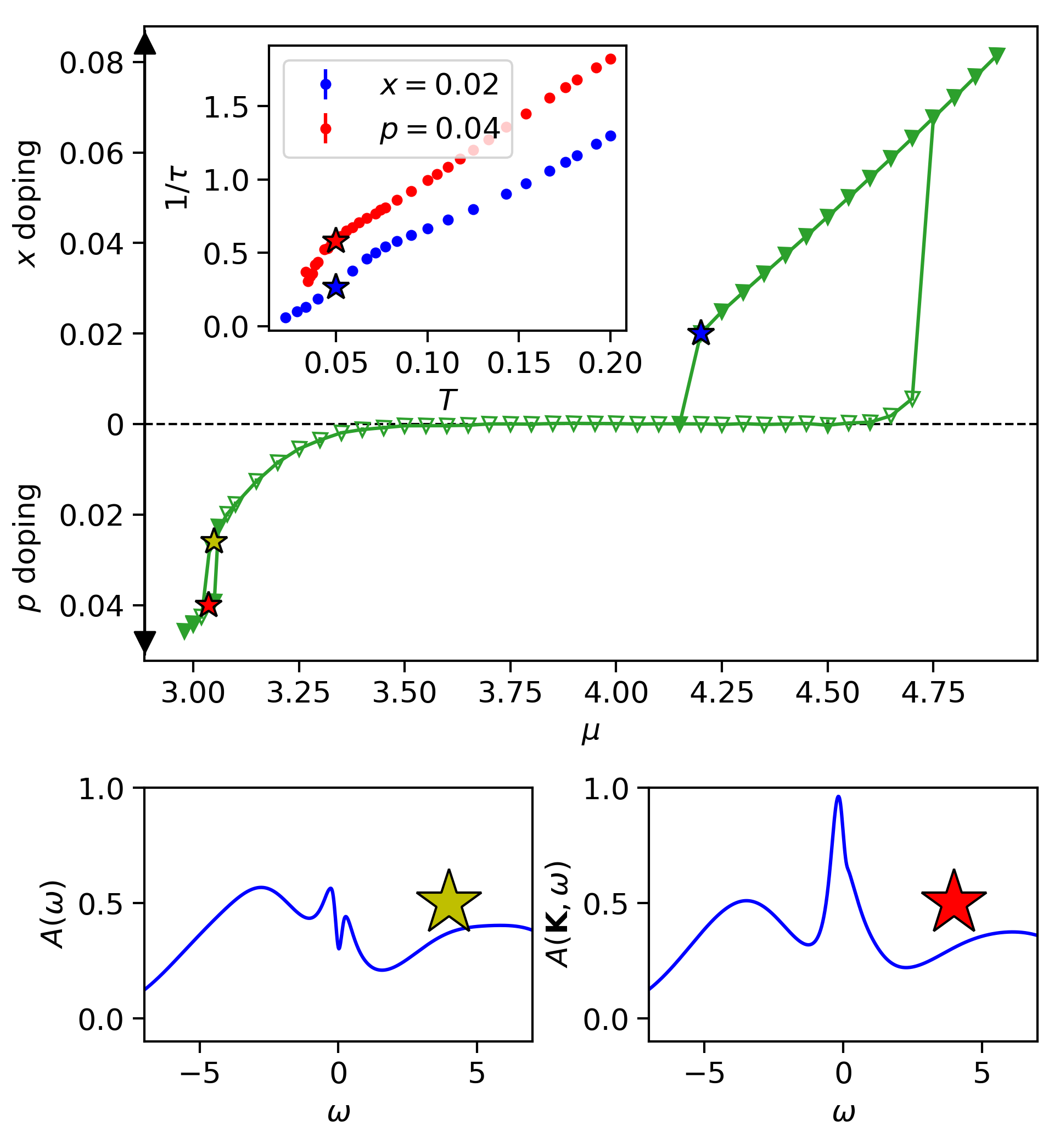
Figure 4: On top, electron doping $x$ and hole doping $p$ as a function of the chemical potential $\mu$ at $T=1/20$ and $U=8.4$. The inset presents the local scattering rate as a function of temperature for $p=0.04$ (red star) and $x=0.02$ (blue star). The scattering rate at $p=0.04$ is larger than at $x=0.02$. Above the position of the star, the temperature dependencies are similar. To illustrate the first-order transition, the bottom row of the plot shows the density of states for the same chemical potential and two coexisting dopings, $p=0.025$ and $p=0.04$, showing a pseudogap in the first case and a quasi-particle peak in the second case.

As stated earlier, $\omega/T$ scaling is usually associated with quantum criticality, but here we do not find it at $p^{*}\sim 0.06$. The procedure to check for $\omega/T$ is explained in Appendix D. We find, $\omega/T$ scaling only at $p=0.04$ for $U=8.4$, and at $p=0.05$ for $U=8.5$. For both values of $U$, this scaling is found only for the first and third patches in a regime where the scattering rate is not linear in $T$ at low temperature. From Figs. 3 and 5 one can verify that the scattering rate at these two dopings are very similar. Indeed, in both cases, there is a downturn of the scattering rate around $T=0.05$ for the first and third patches.

To clarify the origin of the quantum critical point and of $\omega/T$ scaling, consider in Fig. 4 how doping varies as a function of chemical potential $\mu$ at $U=8.4$ and $T=0.05$. There is a first-order transition with coexistence between a pseudogap at $p=0.02$ and a metal $p=0.04$. This can be verified from the density of states computed on both sides of the phase transition with the maximum entropy method, as illustrated on the bottom row of the figure. The loss of spectral weight near the Fermi level is clear on the left plot while the quasiparticle peak is clear on the right plot [58]. There is also a first-order transition on the electron-doped side around $x=0.02$, as shown on the top plot of Fig 4. The inset of that figure shows the local scattering rate $1/\tau(T)$ at $U=8.4$ for both $x=0.02$ and $p=0.04$. On the electron-doped side, just like on the hole-doped side, there is a downturn in $1/\tau$ near $T=0.05$. This suggests that this downturn in $1/\tau(T)$ is intrinsic to the proximity of the first-order transition.

In the case of the square lattice [37, 38], the analog of the first-order Sordi transition that we just discussed is continuously connected to the Mott transition. The first-order Sordi transition on the triangular lattice behaves similarly [39]. In particular, there should be a finite-temperature critical point. In addition, the Mott transition on the square lattice has a quantum-critical point at the end of a coexistence region [15, 71] leading us to suggest that the quantum critical point that we see at $p^{*}=0.06$ on the triangular lattice has a similar origin.

Back to $\omega/T$ scaling. For both $p=0.04$ and $x=0.02$, there is range of $\omega/T$ scaling of the self-energy that breaks down at temperatures below $T\sim 0.05$ for $p=0.04$, and below $T\sim 0.07$ for $x=0.02$. These are the temperatures where the behaviour of the scattering rate in Fig. 4 changes drastically. For the hole-doped case, the critical point of the Sordi transition appears to be near that $T=0.05$ , while it seems to be at a slightly higher temperature for the electron-doped case  . Thus, the $\omega/T$ scaling appears to emerge from the finite-temperature critical point of the Sordi transition.

III.2 Interaction Driven $T$-Linear Scattering Rate

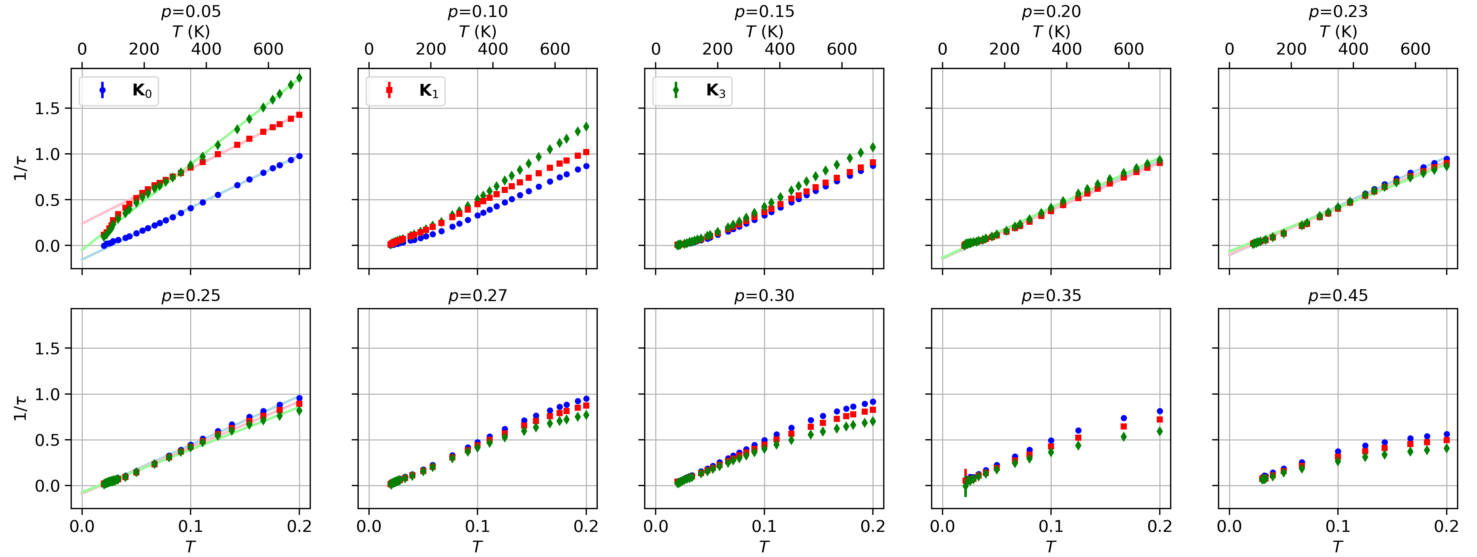
Figure 5: Scattering rate as a function of temperature for a large range of dopings at $U=8.5$ for the zeroth, first and third patches of the triangular lattice in Fig. 1b). A linear fit on the scattering rate as a function of temperature is presented for hole doping between $p=0.05$ and $p=0.45$. For $p=0.5$, the linear fit is done for $T>0.2$. The temperature scale is fixed by taking $t=0.3$eV, typical of the numbers for cuprates.

Before we discuss T-linear scattering, we point out that there is an unusual region in the high doping phase diagram Fig. 2b located between 15% and 20% doping. Indeed, there we find a $T^{2}$ dependence of the scattering rate, a result usually associated to a Fermi liquid. However, because Fermi liquids are usually found at higher dopings and at lower temperature, we suggest that this $T^{2}$ dependence is only an artifact of the cluster that we use. Indeed, in a six-site cluster, an occupation of $n=5/6$ ($p=17\%$) means an odd number of electrons in the cluster. An odd number of electrons increases the entropy, as seen in Ref. (73), which may be the reason why the Mott transition is pushed to higher $U$, as seen in Refs. (73) and (58). Imagine then a situation at some fixed $U$. An odd number of electrons would make interactions less effective because the Mott transition would occur at larger $U$ and because one of the electrons could not form a singlet. This would favour phases such as Fermi liquids instead of other highly correlated phases.

Let us move to $T$-linear scattering at large doping. It is seen in Fig. 2b) below $T\sim 0.03$, for $p$ between $0.2$ and $0.3$. For higher temperatures, the exponent $n$ increases. It is remarkable that the slope of the $T$-linear scattering has been found experimentally [10] to satisfy the relation $\hbar/\tau=\alpha k_{B}T$ with $\alpha\sim 1$. Setting aside the difference between transport scattering time and single-particle scattering time, we note that the value of $\alpha$ is often found experimentally using the Drude formula.

$$\tau_{quasi} =\frac{m^{*}}{ne^{2}\rho}$$ (7)

with $m^{*}$ instead of $m$. In that case the resulting scattering time is the quasiparticle scattering time [74]. In order to compare with our results then, the electron scattering rate $-\text{Im}\Sigma(\omega=0)$ must be multiplied by the quasiparticle weight $Z$, which is obtained from the following relation [75]

$$Z =\left(1-\frac{\partial\Sigma^{\prime}(\omega)}{\partial\omega}\bigg{|}_{\omega\rightarrow 0}\right)^{-1}$$ (8)

$$\approx\left(1-\frac{\text{Im}\Sigma(\omega_{n})}{\omega_{n}}\bigg{|}_{\omega_{n=0}}\right)^{-1}.$$ (9)

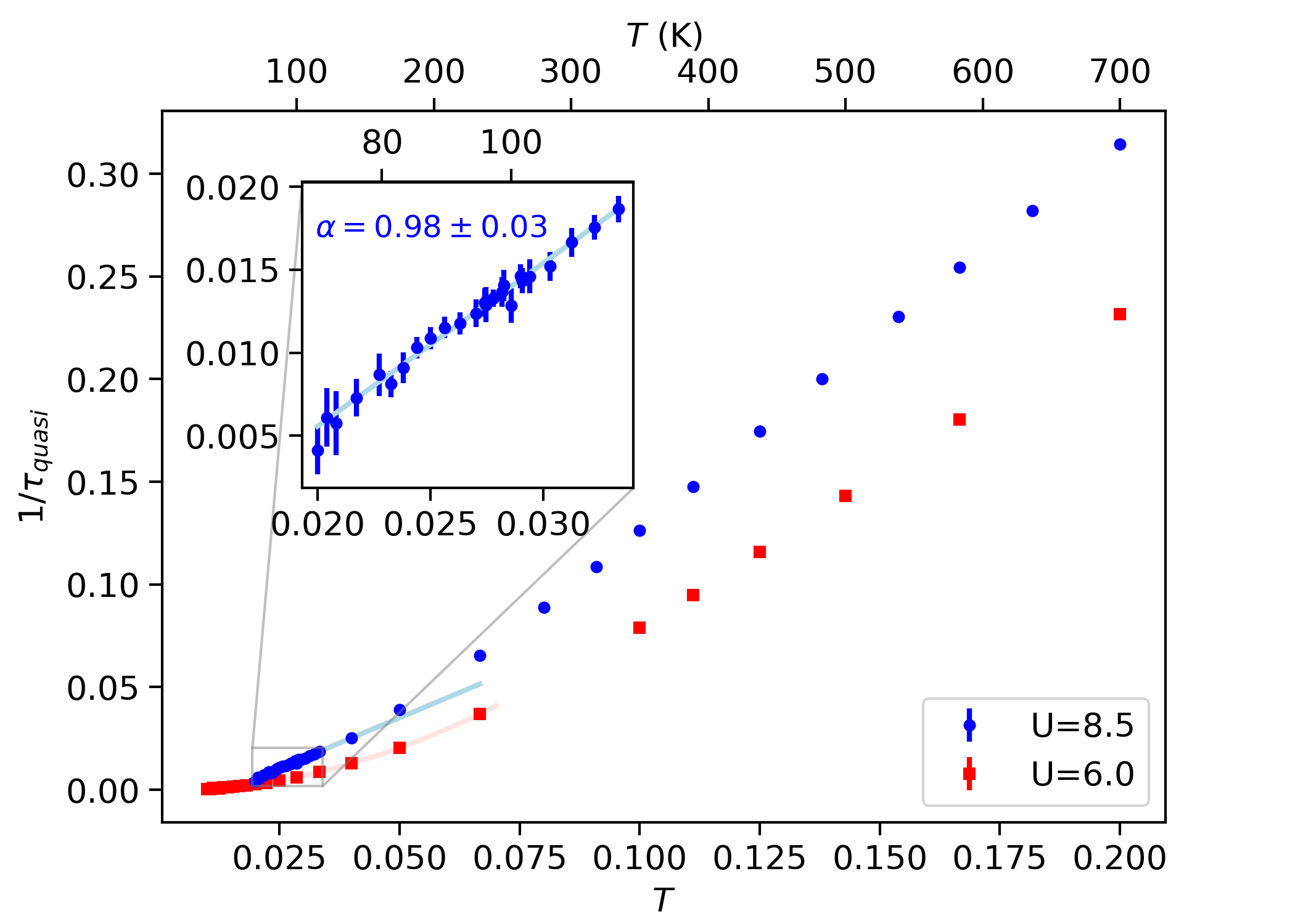
Figure 6: Local quasiparticle scattering rate as a function of temperature at $p=25\%$ and $U=8.5$. A linear fit is performed for temperature between $T=0.02$ and $T=0.03$ in the subplot. The value of $\alpha$ obtained with this fit is presented in the subplot. For $T>1/15$, the slope $\alpha$ increases to $1.89\pm 0.01$. On the other hand, the electron scattering rate $1/\tau$ has a slope $\alpha=3.48\pm 10$ for $T<0.3$.

The local quasiparticle scattering rate at $U=8.5$ as a function of temperature is displayed in Fig. 6. The inset shows a clear linear temperature dependence at low temperature with $\alpha=0.98\pm 0.03$, very close to unity, similarly to the square lattice [12]. Thus, the interaction-driven $T$-linear scattering rate found in the triangular lattice also displays Planckian dissipation. Geometrical frustration then, does not seem to affect the value of $\alpha$ at high doping. Note that the value of $Z$ is about equal to $1/3$ for the data in the inset of Fig. 6. The unrenormalized data is in Fig. 5.

Another characteristic of strange metals is that their self-energy scales with $\omega/T$ [12, 66]. This type of scaling is often related to quantum criticality. Here, we do not find $\omega/T$ scaling. This further asserts the idea that quantum criticality is not responsible for the Planckian dissipation that we see in the high-doping range. We further comment on scaling in Appendix D.

In order to find the origin of Planckian dissipation, the value of $U$ was lowered to see if it would survive. The scattering rates as a function of temperature at $p=0.25$ for both $U=6$ and $U=8.5$ are presented on Fig. 6. We see that at lower $U$, the $T$-linear scattering rate is replaced by a $T^{2}$ scattering rate. This could be expected from an increase in the coherence temperature when $U$ is decreased.

IV Discussion

Strange metallicity is defined by $T$-linear scattering rate for $T\rightarrow 0$. It is usually associated to a quantum critical point at $p^{*}$ [66, 76]. Fig. 5 shows that linear fits of the scattering rate as a function of temperature extrapolate to negative values of $1/\tau$ at $T=0$ for all dopings. Thus, $T$-linear scattering rate has to disappear at $T>0$. The sign problem prevents us to go to low enough temperature to observe that.

As $U$ increases, the finite-temperature critical point of the Sordi transition moves to lower temperature [38]. It may eventually reach zero temperature, in which case it would turn into a quantum critical point and there would be no downturn of the scattering rate. The scattering rate $1/\tau$ would likely extend all the way to $T\to 0$. An analogous quantum-critical point is found at $T=0$ in the two orbital Hubbard model with Hund coupling [77].

That the interaction-driven $T$-linear scattering rate is found for a wide range of dopings, $0.2<p<0.3$, suggests that it does not emerge from a quantum-critical point. This is supported by the lack of $\omega/T$ scaling. The extrapolation of the linear behavior to negative temperatures at $T=0$ suggests instead a crossover from linear to Fermi liquid $T^{2}$ at a temperature lower than what is computationally achievable with DCA. Such a crossover is visible at $U=6$ in Fig. 6. The crossover temperature decreases as $U$ increases.

Note that the interaction-driven $T$-linear scattering rate that we find here is similar to what is found on the 8-site square lattice with DCA where, however, $\omega/T$ scaling was found at one doping and connected to the effect of spin fluctuations [12].

Since $\omega/T$ scaling is not found in the interaction-driven $T$-linear scattering rate, we look for other possible scalings. We find in Appendix D that $\text{Im}\left(\Sigma(i\omega_{n}),\mathbf{K}_{3}\right)/\left(\text{Im}\Sigma(i\omega_{n}=0,\mathbf{K}_{3})\right)$ scales like $\omega/T^{z}$, where $z$ varies between $2$ and $2.3$ depending on the doping and the patch. This type of scaling of the self-energy is different to what is expected from both Fermi liquid theory, where $-\text{Im}\Sigma\sim\omega^{2}+T^{2}$, and quantum-critical strange metals. The scaling encountered in this $T$-linear scattering rate region is also dimensionful, which means that it is non-universal. We do not have any explanation for this type of scaling.

A brief comparison with cuprates: We saw that the interaction-driven $T$-linear scattering rate is lost at temperatures higher than $T\sim 0.03$ where the exponent of the $T$ dependence increases. This kind of deviation from $T$-linear scattering rate is commonly found in LCCO, PCCO, Nd-LSCO and Bi2212 [78, 22]. Even though a direct comparison with cuprates is not warranted, we mention that the temperature at which the $T$-linear scattering rate is lost on the triangular lattice ($T\sim 150K$) is similar to what is found in Nd-LSCO and Bi2212 ($T\sim 120$K) [22]. Also, as in cuprates, the scattering rate in the interaction-driven $T$-linear scattering rate region is near isotropic [23]. Note that the cuprate measurements, however, were done close to a van Hove singularity. Another similarity between the strange metal found in cuprates and the interaction-driven $T$-linear scattering rate is that both display Planckian dissipation. This means that geometrical frustration does not change the slope. Moreover, Fig. 6 shows that $T$-linear scattering rate disappears at low $U$. Thus, Planckian dissipation occurs when interactions are sufficiently strong, with no obvious other explanations.

There are important differences between what is found here on the triangular lattice and what is found in cuprates like LSCO. Cuprates have a $T$-linear scattering rate on a wide range of dopings like we find, but linearity extends down to $T\rightarrow 0$ on the entire range of dopings [10]. Moreover, they exhibit $\omega/T$ scaling for dopings away from $p^{*}$ [79].

In real materials like cuprates, the effect of disorder may be important for observing linear in $T$ scattering rate, as emphasized in quantum-critical models [80], in SYK models [81] or much earlier in Boltzmann transport [82, 83]. In the latter case, Rosch [82] pointed out that disorder may invalidate the Hlubina-Rice argument [83] that Fermi-liquid like regions of the Fermi surface with $T^{2}$ scattering rate would short-circuit hot-spots with $T$ scattering rate. With disorder, the Hlubina-Rice argument can indeed be invalid. Using a caricature to account for an elastic scattering rate $\Gamma_{0}$ with Mathiessen’s rule, one finds that as $T$ approaches zero, $\Gamma_{0}$ becomes larger than $T^{2}$ faster than it becomes larger than $T$. The effect of disorder on scattering rate remains to be studied with DCA.

Research on the triangular Hubbard model allows to discriminate the effect of long- vs short-range AFM fluctuations. Finding $T$-linear scattering rate in this model shows that only short-range fluctuations are important, particularly since many studies do not find magnetic ordering at half filling in the range of interaction strength we studied [40, 41, 42, 43, 44, 45, 46].

V Conclusion

We used DCA with a CT-AUX continuous-time impurity solver to study $T$-linear scattering rate in the hole-doped triangular-lattice Hubbard model. We find that the phase diagram displays two metallic regions with linear in $T$ scattering rates. The first one, that we call Mott-driven, is found for low dopings near the Sordi transition. This $T$-linear scattering rate has $\omega/T$ scaling and emerges from a single doping $p^{*}\sim 0.06$. The second $T$-linear scattering rate region, that we call interaction-driven $T$-linear scattering rate, has no $\omega/T$ scaling and is found for a wide range of dopings. It does not emerge from a quantum-critical point. The linear fits of the scattering rate as a function of temperature extrapolate to negative value of $1/\tau$ at $T=0$, which suggests a crossover to a Fermi liquid regime at a temperature lower than what is actually possible to achieve because of the sign problem. Although it does not have a quantum critical point, we found Planckian dissipation in this regime of interaction-driven $T$-linear scattering rate at $p=0.25$.

This study is the first to report that there might be two different regimes for $T$-linear scattering in strongly correlated materials. This discovery may have an impact on our current understanding of strongly correlated materials, and more particularly, could impact our vision of the strange metal in cuprates. It would thus be important to verify if other models, or calculation technique, find $T$-linear scattering rate without quantum criticality and phonon interactions or near the Sordi transition.

VI Acknowledgements

Useful discussions with P.A. Graham, L. Taillefer and G. Grissonnanche are acknowledged. This work has been supported by the Natural Sciences and Engineering Research Council of Canada (NSERC) under grant RGPIN-2019-05312 and by the Canada First Research Excellence Fund. The calculation resources were provided by Calcul-Québec and the Digital Research Alliance of Canada.

Appendix A 12 sites DCA

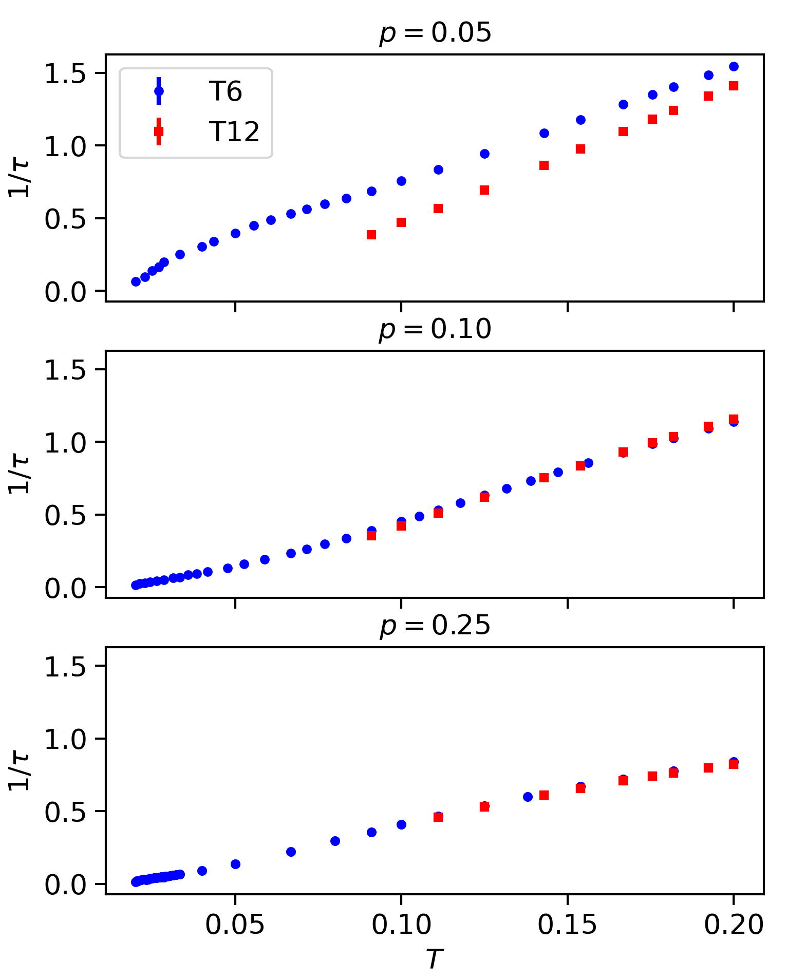
Figure 7: Local scattering rate as a function of temperature for $U=8.5$ and three dopings, $p=0.05$, $p=0.1$ and $p=0.25$, for the six-site bipartite cluster in blue and the twelve-site bipartite cluster in red.

To verify the accuracy of our results, the scattering rate as a function of temperature with a 12 site bipartite cluster was computed with DCA for the two values $U=8.4$ and $U=8.5$. The results obtained for $U=8.5$ are presented at Fig. 7. The 12-site bipartite-cluster results are very similar to those of the 6-site cluster for high dopings. At lower dopings, it is not the case anymore.

One can understand why by looking at Fig. 8. Results for the Widom line indicate that the Mott transition is at larger $U$ in the 12-site cluster. With the Mott transition for the 12-site cluster at much larger $U$, effects from the Sordi transition on the scattering rate do not appear at low doping. Hence, we should not expect results at low dopings to be the same for both of those clusters. Furthermore,because of the sign problem, it is impossible to get accurate results below $\beta=11$ on the 12-site cluster, which means that it is not possible to verify our results at the lowest temperatures.

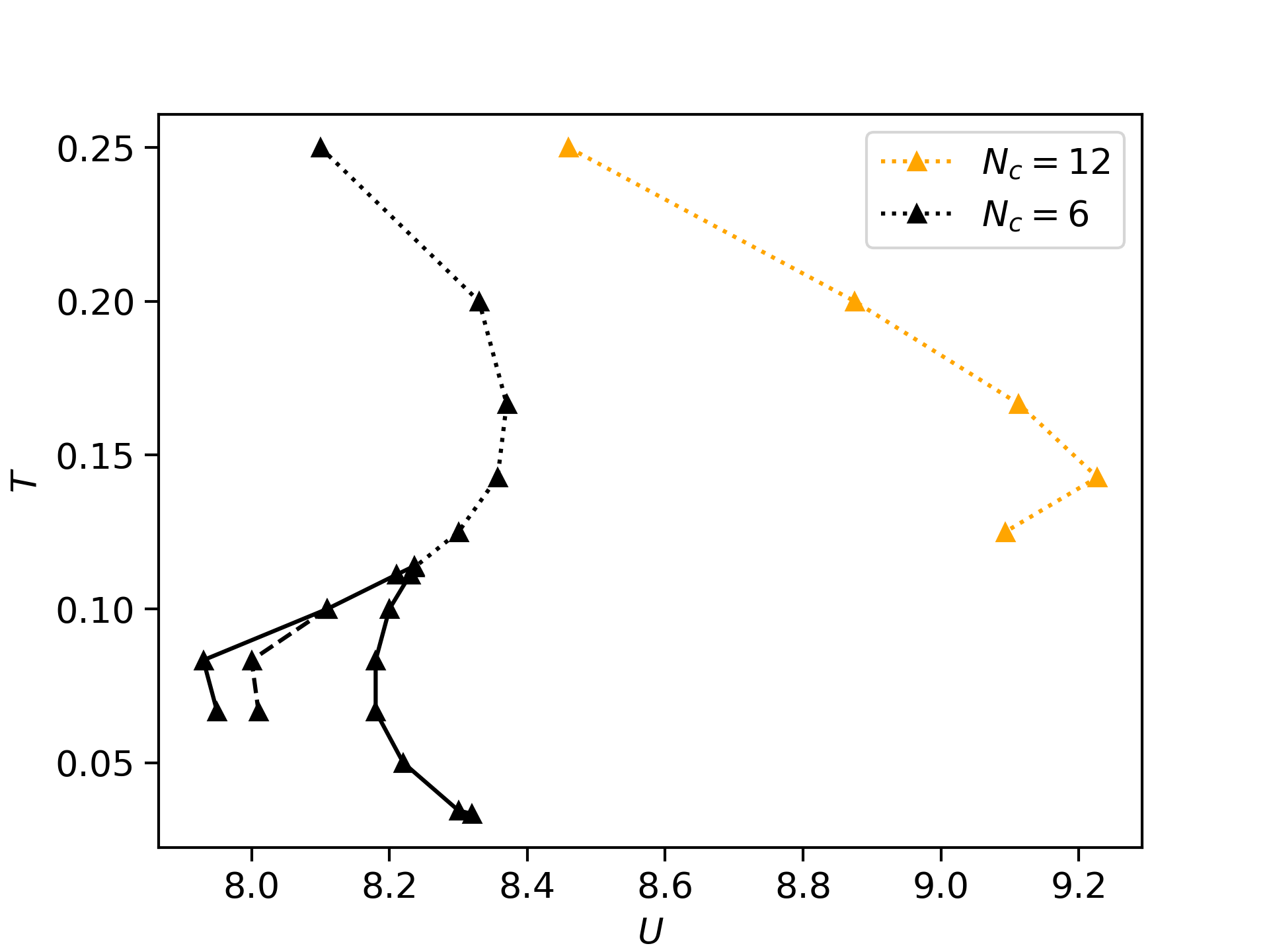
Figure 8: Mott transition and Widom line for six-site and twelve-site clusters of the triangular lattice. The dotted line corresponds to the Widom line [84], a crossover. The solid lines correspond to $U_{c1}$ and $U_{c2}$ for the Mott transitions, and the dashed line corresponds to $U_{c3}$.

Appendix B Polynomial fit on first Matsubara frequencies

Much of the literature uses a polynomial fit on the first Matsubara frequencies to find the approximate value of a given observable at $\omega=0$. This is usually a good approximation [12]. Testing and comparing low frequency results from such techniques, we conclude that the best polynomial fit is of order three.

We also compared with maximum-entropy analytic continuation [85] and with a second degree least-square regression on the first six Matsubara frequencies. The results for the second degree least-square regression are in concordance with the second degree polynomial fit. Although the results at order 4 better fit the maximum-entropy technique, as seen on Fig. 9, it is prone to small errors in the input observables. Since the shape of the final fit does not change much, this indicates that the results given in the article are valid.

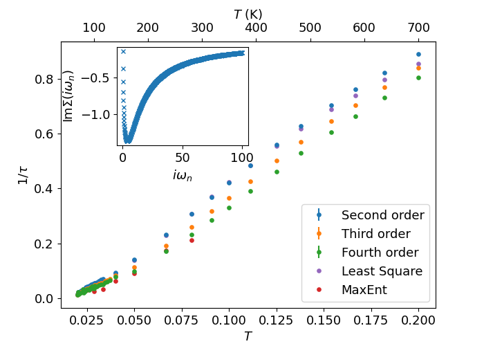
Figure 9: Local scattering rate ($\text{-Im}\Sigma(\omega=0)$) as a function of temperature $T$ for $p=0.25$ and $U=8.5$ obtained from the Matsubara self-energy using polynomial fits of different orders. Also shown is a second order least-square regression on the first six Matsubara frequencies and $\text{Im}\Sigma(\omega=0)$ obtained with the MaxEnt method OmegaMaxEnt [85]. The inset displays the imaginary part of the self-energy as a function of the Matsubara frequencies for $T=0.02$, $p=0.25$ and $U=8.5$

B.1 Planckian dissipation

The slope of the scattering rate as a function of temperature decreases when the order of the polynomial fit increases. To verify if the quasiparticle scattering rate is still Planckian with higher-order polynomial fits of the self-energy, the slope of the quasiparticle scattering rate as a function of temperature was computed for polynomial fits of higher order. We find slopes $\alpha=0.87\pm 0.04$ and $\alpha=0.78\pm 0.02$ with polynomial fits of order four and five respectively. These values of $\alpha$ are still within the slope found experimentally in materials displaying Planckian behaviour [22]. Thus, even if the slope of the quasiparticle scattering rate depends on the order of the polynomial fit on the Matsubara frequencies, we find that the $\alpha$ obtained remains close to the Planckian limit of $\alpha=1$ in the interaction-driven $T$-linear scattering rate.

One should note that the results from the maximum entropy analytic continuation are not very stable in temperature, so we did not push our analysis further for this.

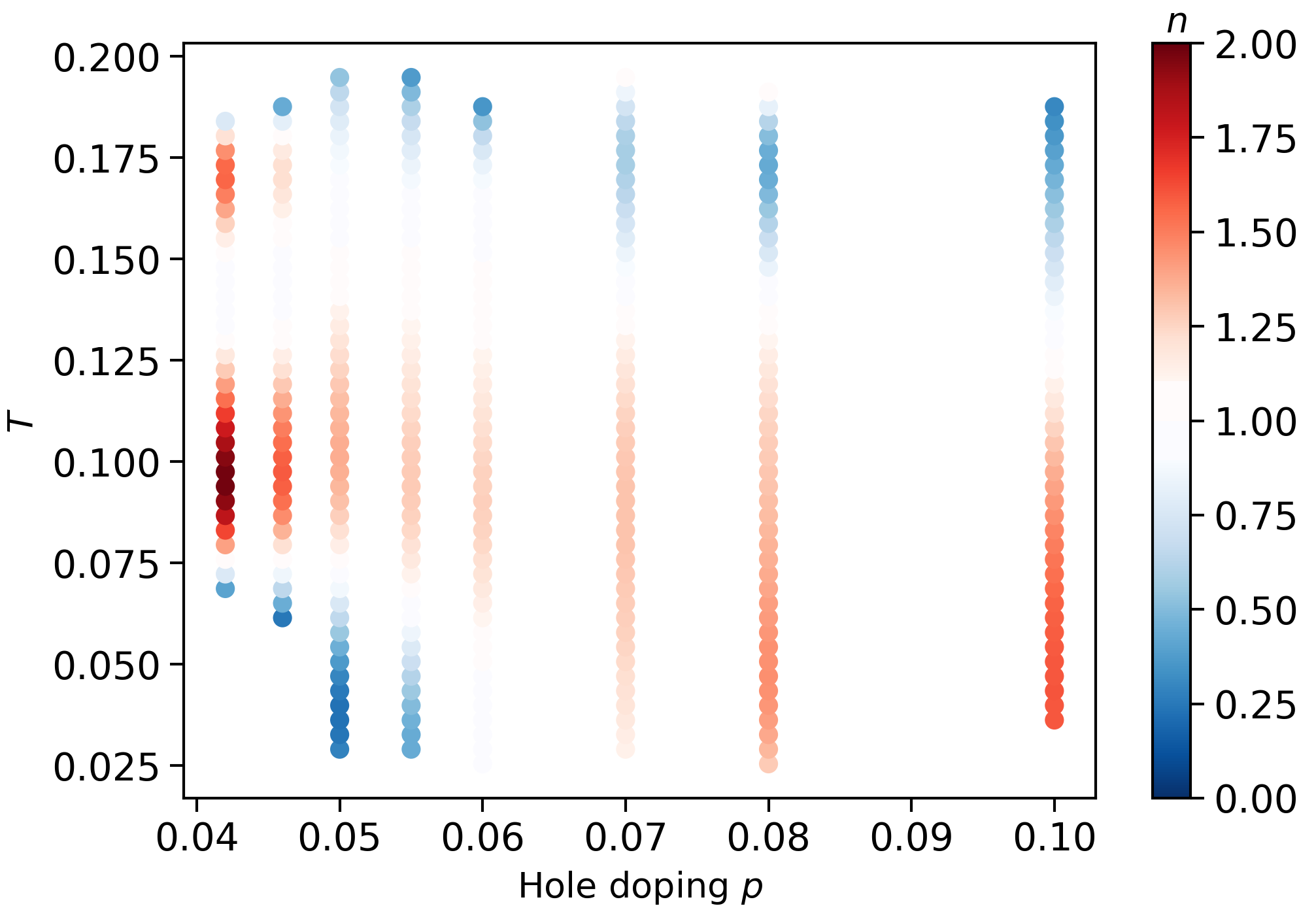
Figure 10: Raw data for the temperature-doping phase diagram Fig. 2a) of the local scattering rate for $U=8.4$. The value of $n$ obtained from a fit of the form $1/\tau=\alpha T^{n}+b$ of the local scattering rate is color coded and interpolated to obtain Fig. 2a).

Appendix C Phase Diagram

To obtain the phase diagrams in Fig. 2, the scattering rate as a function of temperature for the different dopings were fitted using Legendre polynomials of degree 7. Then, a fit of the form $aT^{n}+b$ was performed on each group of 10 points of the Legendre fit to obtain the local value of $n$ as a function of temperature and doping. The values of $n$ were then interpolated on a meshgrid to obtain Fig. 2. The non-interpolated values of $n$ are presented on Fig. 10. At low dopings and low temperature, the scattering rate could not be fitted with the form $aT^{n}+b$, hence the absence of points. Different orders of the Legendre polynomial and number of points for the fits were tested to make sure that the values of $n$ color coded on the figure were independent of these parameters.

Appendix D $\omega/T$ scaling

Most strange metals have an optical conductivity that scales like $\omega/T$ or, alternatively, a self-energy that has the form $-\text{Im}\Sigma(i\omega_{n},T)=\lambda T^{\nu}\Phi(\frac{i\omega_{n}}{T})$, where $\lambda$ is some constant and $\Phi$ is a function of $i\omega_{n}/T$ [66, 35]. The $\omega/T$ scaling is then obtained from analytic continuation $i\omega_{n}\rightarrow\omega+i\eta$. This type of scaling is normally associated with quantum-critical points.

We can verify whether our data follows $i\omega_{n}/T$ scaling by computing $\text{Im}\Sigma(i\omega_{n},T)/\text{Im}\Sigma(i\omega_{n}=0,T)$ that should then scale as $\Phi(\frac{i\omega_{n}}{T})/\Phi(0)$. There are two regimes of doping with linear in $T$ scattering. Let us begin with the large doping regime. There is T-linear scattering rate for $p=0.25$ and $T<\frac{1}{33}$. The above ratio as a function of $i\omega_{n}/T$ is presented on Fig. 11 for the first patch. We find that the self-energy for all patches in this interaction-driven $T$-linear scattering rate does not display $\omega/T$ scaling. The absence of $\omega/T$ scaling, along with the existence of Planckian dissipation for a large range of dopings, leads us to conclude that $T$-linear scattering here does not emerge from quantum criticality.

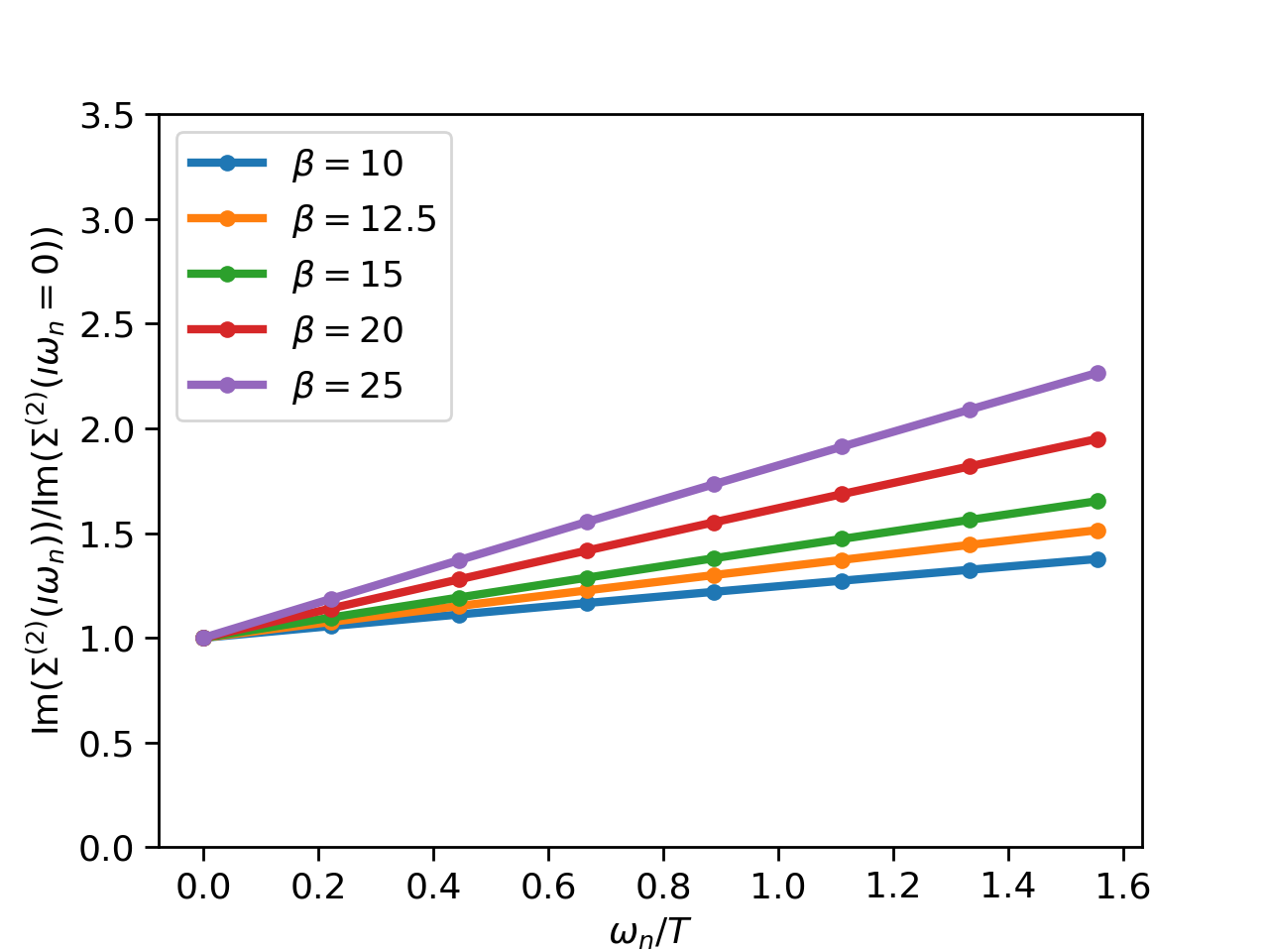
Figure 11: $\text{Im}\left(\Sigma(i\omega_{n}),\mathbf{K}_{1}\right)/\left(\text{Im}\Sigma(i\omega_{n}=0),\mathbf{K}_{1}\right)$ as a function of $\omega_{n}/T$ for temperatures where a T-linear scattering rate is found at $p=0.25$. Only the small values of $\omega_{n}/T$ are displayed in order to verify the $\omega/T$ scaling.

There is however a finite temperature critical point at $p=0.04$ for $U=8.4$. $\Sigma(i\omega_{n},T)/\Sigma(i\omega_{n}=0,T)$ as a function of $i\omega_{n}/T$ for this doping is presented at Fig. 12. We see that, for temperatures higher than the finite-temperature of the critical point, the Mott-driven $T$-linear scattering rate displays $\omega/T$ scaling.

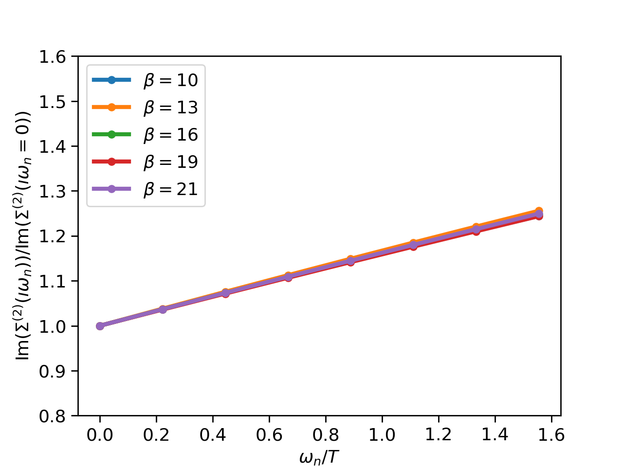
Figure 12: $\text{Im}\left(\Sigma(i\omega_{n},\mathbf{K}_{1})\right)$/ $\left(\text{Im}\Sigma(i\omega_{n}=0,\mathbf{K}_{1})\right)$ as a function of $\omega_{n}/T$ for temperatures where a T-linear scattering rate is found at $p=0.04$ and $U=8.4$. Only the small values of $\omega_{n}/T$ are displayed in order to verify the $\omega/T$ scaling.

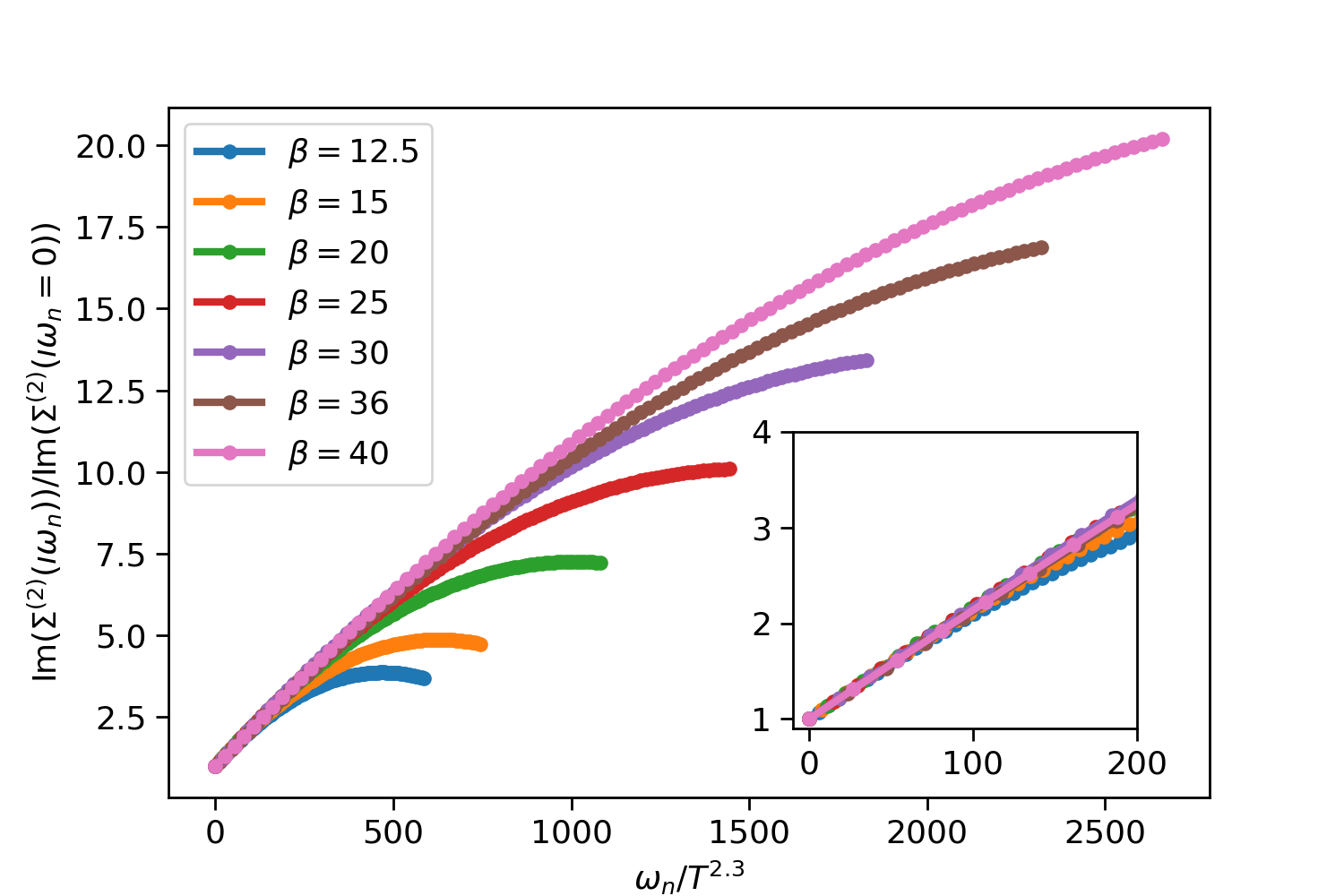
Figure 13: $\text{Im}\left(\Sigma(i\omega_{n}),\mathbf{K}_{3}\right)/\left(\text{Im}\Sigma(i\omega_{n}=0,\mathbf{K}_{3})\right)$ as a function of $\omega_{n}/T^{2.3}$ for different temperatures for doping $p=0.25$. The insert shows the low-temperature scaling.

To find out whether there is a different scaling of the self-energy in the interaction-driven $T$-linear scattering we computed $\Sigma(i\omega_{n},T)/\Sigma(i\omega_{n}=0,T)$ as a function of $\omega/T^{z}$. The value of $z$ was varied until each temperature has the same scaling of $\Sigma(i\omega_{n},T)/\Sigma(i\omega_{n}=0,T)$ at low Matsubara frequency. We find $\omega/T^{2.3}$ scaling, as shown in Fig. 13.

References

- Cao et al. [2020] Yuan Cao, Debanjan Chowdhury, Daniel Rodan-Legrain, Oriol Rubies-Bigorda, Kenji Watanabe, Takashi Taniguchi, T. Senthil, and Pablo Jarillo-Herrero, “Strange Metal in Magic-Angle Graphene with near Planckian Dissipation,” Physical Review Letters 124, 076801 (2020).
- Polshyn et al. [2019] Hryhoriy Polshyn, Matthew Yankowitz, Shaowen Chen, Yuxuan Zhang, K. Watanabe, T. Taniguchi, Cory R. Dean, and Andrea F. Young, “Large linear-in-temperature resistivity in twisted bilayer graphene,” Nature Physics 15, 1011–1016 (2019).
- Cha et al. [2021] Peter Cha, Aavishkar A. Patel, and Eun-Ah Kim, “Strange Metals from Melting Correlated Insulators in Twisted Bilayer Graphene,” Physical Review Letters 127, 266601 (2021).
- [4] Augusto Ghiotto, En-Min Shih, Bumho Kim, Jiawei Zang, Andrew J Millis, Kenji Watanabe, Takashi Taniguchi, James C Hone, Lei Wang, Cory R Dean, and Abhay N Pasupathy, “Quantum Criticality in Twisted Transition Metal Dichalcogenides,” , 18.
- Doiron-Leyraud et al. [2009] Nicolas Doiron-Leyraud, Pascale Auban-Senzier, Samuel René de Cotret, Claude Bourbonnais, Denis Jérome, Klaus Bechgaard, and Louis Taillefer, “Correlation between linear resistivity and T c in the Bechgaard salts and the pnictide superconductor Ba ( Fe1-x Co x )2 As2,” Physical Review B 80, 214531 (2009).
- [6] J. Custers, P. Gegenwart, H. Wilhelm, K. Neumaier, Y. Tokiwa, O. Trovarelli, C. Geibel, F. Steglich, C. Pépin, and P. Coleman, “The break-up of heavy electrons at a quantum critical point,” 424, 524–527.
- [7] R. Daou, C. Bergemann, and S. R. Julian, “Continuous Evolution of the Fermi Surface of ${\mathrm{CeRu}}_{2}{\mathrm{Si}}_{2}$ across the Metamagnetic Transition,” 96, 026401.
- [8] Valentina Martelli, Ang Cai, Emilian M. Nica, Mathieu Taupin, Andrey Prokofiev, Chia-Chuan Liu, Hsin-Hua Lai, Rong Yu, Kevin Ingersent, Robert Küchler, André M. Strydom, Diana Geiger, Jonathan Haenel, Julio Larrea, Qimiao Si, and Silke Paschen, “Sequential localization of a complex electron fluid,” 116, 17701–17706.
- Ayres et al. [2021] J. Ayres, M. Berben, M. Čulo, Y.-T. Hsu, E. van Heumen, Y. Huang, J. Zaanen, T. Kondo, T. Takeuchi, J. R. Cooper, C. Putzke, S. Friedemann, A. Carrington, and N. E. Hussey, “Incoherent transport across the strange-metal regime of overdoped cuprates,” Nature 595, 661–666 (2021).
- Cooper et al. [2009] R. A. Cooper, Y. Wang, B. Vignolle, O. J. Lipscombe, S. M. Hayden, Y. Tanabe, T. Adachi, Y. Koike, M. Nohara, H. Takagi, Cyril Proust, and N. E. Hussey, “Anomalous Criticality in the Electrical Resistivity of La Sr CuO ,” Science 323, 603–607 (2009).
- Singh [2021] Navinder Singh, “Leading theories of the cuprate superconductivity: A critique,” Physica C: Superconductivity and its Applications 580, 1353782 (2021).
- Wú et al. [2022] Wéi Wú, Xiang Wang, and André-Marie Tremblay, “Non-fermi liquid phase and linear-in-temperature scattering rate in overdoped two-dimensional hubbard model,” Proceedings of the National Academy of Sciences 119, e2115819119 (2022).
- Cha et al. [2020] Peter Cha, Nils Wentzell, Olivier Parcollet, Antoine Georges, and Eun-Ah Kim, “Linear resistivity and Sachdev-Ye-Kitaev (SYK) spin liquid behavior in a quantum critical metal with spin-1/2 fermions,” Proceedings of the National Academy of Sciences 117, 18341–18346 (2020).
- Poniatowski et al. [2021] Nicholas R. Poniatowski, Tarapada Sarkar, Ricardo P. S. M. Lobo, Sankar Das Sarma, and Richard L. Greene, “Counterexample to the conjectured Planckian bound on transport,” Physical Review B 104, 235138 (2021).
- Vučičević et al. [2015] J. Vučičević, D. Tanasković, M.J. Rozenberg, and V. Dobrosavljević, “Bad-Metal Behavior Reveals Mott Quantum Criticality in Doped Hubbard Models,” Physical Review Letters 114, 246402 (2015).
- Brown et al. [2018] Peter T. Brown, Debayan Mitra, Elmer Guardado-Sanchez, Reza Nourafkan, Alexis Reymbaut, Charles-David Hébert, Simon Bergeron, A.-M. S. Tremblay, Jure Kokalj, David A. Huse, Peter Schauss, and Waseem S. Bakr, “Bad metallic transport in a cold atom fermi-hubbard system,” Science (2018), 10.1126/science.aat4134.
- Vučičević et al. [2019] J. Vučičević, J. Kokalj, R. Žitko, N. Wentzell, D. Tanasković, and J. Mravlje, “Conductivity in the Square Lattice Hubbard Model at High Temperatures: Importance of Vertex Corrections,” Physical Review Letters 123, 036601 (2019).
- Gurvitch and Fiory [1987] M. Gurvitch and A. T. Fiory, “Resistivity of La1.825Sr0.175CuO4 and YBa2Cu3O7 to 1100 K: Absence of saturation and its implications,” Phys. Rev. Lett. 59, 1337–1340 (1987).
- Takagi et al. [1992] H. Takagi, B. Batlogg, H. L. Kao, J. Kwo, R. J. Cava, J. J. Krajewski, and W. F. Peck, “Systematic evolution of temperature-dependent resistivity in La 2-x Sr x CuO 4,” Physical Review Letters 69, 2975–2978 (1992).
- Zaanen [2004] Jan Zaanen, “Why the temperature is high,” Nature 430, 512–513 (2004).
- Bruin et al. [2013] J. A. N. Bruin, H. Sakai, R. S. Perry, and A. P. Mackenzie, “Similarity of Scattering Rates in Metals Showing T-Linear Resistivity,” Science 339, 804–807 (2013).
- Legros et al. [2019] A. Legros, S. Benhabib, W. Tabis, F. Laliberté, M. Dion, M. Lizaire, B. Vignolle, D. Vignolles, H. Raffy, Z. Z. Li, P. Auban-Senzier, N. Doiron-Leyraud, P. Fournier, D. Colson, L. Taillefer, and C. Proust, “Universal T-linear resistivity and Planckian dissipation in overdoped cuprates,” Nature Physics 15, 142–147 (2019).
- Grissonnanche et al. [2021] Gaël Grissonnanche, Yawen Fang, Anaëlle Legros, Simon Verret, Francis Laliberté, Clément Collignon, Jianshi Zhou, David Graf, Paul A. Goddard, Louis Taillefer, and B. J. Ramshaw, “Linear-in temperature resistivity from an isotropic Planckian scattering rate,” Nature 595, 667–672 (2021).
- Hartnoll and Mackenzie [2022] Sean A. Hartnoll and Andrew P. Mackenzie, “Colloquium : Planckian dissipation in metals,” Reviews of Modern Physics 94, 041002 (2022).
- Li and She [2021] Rong Li and Zhen-Su She, “Emergent mesoscopic quantum vortex and Planckian dissipation in the strange metal phase,” New Journal of Physics 23, 043050 (2021).
- Lee [2021] Patrick A. Lee, “Low-temperature T -linear resistivity due to umklapp scattering from a critical mode,” Physical Review B 104, 035140 (2021).
- Rice et al. [2017] T. Maurice Rice, Neil J. Robinson, and Alexei M. Tsvelik, “Umklapp scattering as the origin of T -linear resistivity in the normal state of high- T c cuprate superconductors,” Physical Review B 96, 220502 (2017).
- Patel and Sachdev [2019] Aavishkar A. Patel and Subir Sachdev, “Theory of a Planckian metal,” Physical Review Letters 123, 066601 (2019).
- Robinson et al. [2019] Neil J Robinson, Peter D Johnson, T Maurice Rice, and Alexei M Tsvelik, “Anomalies in the pseudogap phase of the cuprates: competing ground states and the role of umklapp scattering,” Reports on Progress in Physics 82, 126501 (2019).
- Varma [2020] Chandra M. Varma, “Colloquium : Linear in temperature resistivity and associated mysteries including high temperature superconductivity,” Reviews of Modern Physics 92, 031001 (2020).
- Zaanen [2019] Jan Zaanen, “Planckian dissipation, minimal viscosity and the transport in cuprate strange metals,” SciPost Physics 6, 061 (2019).
- Else et al. [2021] Dominic V. Else, Ryan Thorngren, and T. Senthil, “Non-Fermi liquids as ersatz Fermi liquids: general constraints on compressible metals,” Physical Review X 11, 021005 (2021).
- Else and Senthil [2021] Dominic V. Else and T. Senthil, “Strange metals as ersatz Fermi liquids,” Physical Review Letters 127, 086601 (2021).
- Ding et al. [2017] Wenxin Ding, Rok Žitko, Peizhi Mai, Edward Perepelitsky, and B. Sriram Shastry, “Strange metal from Gutzwiller correlations in infinite dimensions,” Physical Review B 96, 054114 (2017).
- Georges and Mravlje [2021] Antoine Georges and Jernej Mravlje, “Skewed Non-Fermi Liquids and the Seebeck Effect,” Physical Review Research 3, 043132 (2021).
- Maier et al. [2005] Thomas Maier, Mark Jarrell, Thomas Pruschke, and Matthias H. Hettler, “Quantum cluster theories,” Reviews of Modern Physics 77, 1027–1080 (2005).
- Sordi et al. [2010] Giovanni Sordi, Kristjan Haule, and A-MS Tremblay, “Finite doping signatures of the mott transition in the two-dimensional hubbard model,” Physical review letters 104, 226402 (2010).
- Sordi et al. [2011] G. Sordi, K. Haule, and A.-M. S. Tremblay, “Mott physics and first-order transition between two metals in the normal-state phase diagram of the two-dimensional hubbard model,” Phys. Rev. B 84, 075161 (2011).
- Downey et al. [2023a] P. O. Downey, O. Gingras, C. D. Hébert, M. Charlebois, and A. M. S. Tremblay, “Filling-induced mott transition and pseudogap physics in the triangular lattice hubbard model,” (2023a), arXiv:2307.11190 [cond-mat.str-el] .
- Sahebsara and Sénéchal [2008] Peyman Sahebsara and David Sénéchal, “Hubbard Model on the Triangular Lattice: Spiral Order and Spin Liquid,” Phys. Rev. Lett. 100, 136402 (2008).
- Laubach et al. [2015] Manuel Laubach, Ronny Thomale, Christian Platt, Werner Hanke, and Gang Li, “Phase diagram of the Hubbard model on the anisotropic triangular lattice,” Physical Review B 91, 245125 (2015).
- Misumi et al. [2017] Kazuma Misumi, Tatsuya Kaneko, and Yukinori Ohta, “Mott transition and magnetism of the triangular-lattice hubbard model with next-nearest-neighbor hopping,” Phys. Rev. B 95, 075124 (2017).
- Tocchio et al. [2008] Luca F. Tocchio, Federico Becca, Alberto Parola, and Sandro Sorella, “Role of backflow correlations for the nonmagnetic phase of the hubbard model,” Phys. Rev. B 78, 041101 (2008).
- Yoshioka et al. [2009] Takuya Yoshioka, Akihisa Koga, and Norio Kawakami, “Quantum phase transitions in the hubbard model on a triangular lattice,” Phys. Rev. Lett. 103, 036401 (2009).
- Wietek et al. [2021] Alexander Wietek, Riccardo Rossi, Fedor Šimkovic, Marcel Klett, Philipp Hansmann, Michel Ferrero, E. Miles Stoudenmire, Thomas Schäfer, and Antoine Georges, “Mott Insulating States with Competing Orders in the Triangular Lattice Hubbard Model,” Phys. Rev. X 11, 041013 (2021).
- Yu et al. [2023] Yang Yu, Shaozhi Li, Sergei Iskakov, and Emanuel Gull, “Magnetic phases of the anisotropic triangular lattice hubbard model,” Physical Review B 107, 075106 (2023).
- Oike et al. [2017] Hiroshi Oike, Yuji Suzuki, Hiromi Taniguchi, Yasuhide Seki, Kazuya Miyagawa, and Kazushi Kanoda, “Anomalous metallic behaviour in the doped spin liquid candidate -(ET)4Hg2.89Br8,” Nature Communications 8, 756 (2017).
- Yoshimoto et al. [2013] Ryo Yoshimoto, Akihito Naito, Satoshi Yamashita, and Yasuhiro Nakazawa, “Antiferromagnetic fluctuations and proton Schottky heat capacity in doped organic conductor -(BEDT-TTF)4Hg2.78Cl8,” Physica B: Condensed Matter 427, 1–4 (2013).
- Yamamoto et al. [2013] Hiroshi M. Yamamoto, Masaki Nakano, Masayuki Suda, Yoshihiro Iwasa, Masashi Kawasaki, and Reizo Kato, “A strained organic field-effect transistor with a gate-tunable superconducting channel,” Nature Communications 4, 2379 (2013).
- Ming et al. [2017] Fangfei Ming, Steve Johnston, Daniel Mulugeta, Tyler S. Smith, Paolo Vilmercati, Geunseop Lee, Thomas A. Maier, Paul C. Snijders, and Hanno H. Weitering, “Realization of a Hole-Doped Mott Insulator on a Triangular Silicon Lattice,” Physical Review Letters 119, 266802 (2017).
- Tarruell and Sanchez-Palencia [2018] Leticia Tarruell and Laurent Sanchez-Palencia, “Quantum simulation of the Hubbard model with ultracold fermions in optical lattices,” Comptes Rendus Physique Quantum simulation / Simulation quantique, 19, 365–393 (2018).
- Yang et al. [2021] Jin Yang, Liyu Liu, Jirayu Mongkolkiattichai, and Peter Schauss, “Site-resolved imaging of ultracold fermions in a triangular-lattice quantum gas microscope,” PRX Quantum 2, 020344 (2021).
- Mongkolkiattichai et al. [2022] Jirayu Mongkolkiattichai, Liyu Liu, Davis Garwood, Jin Yang, and Peter Schauss, “Quantum gas microscopy of a geometrically frustrated hubbard system,” (2022), arXiv:2210.14895 [cond-mat.quant-gas] .
- [54] Daniel P Arovas, Erez Berg, Steven A Kivelson, and Srinivas Raghu, “The Hubbard Model,” .
- Qin et al. [2022] Mingpu Qin, Thomas Schäfer, Sabine Andergassen, Philippe Corboz, and Emanuel Gull, “The Hubbard Model: A Computational Perspective,” Annual Review of Condensed Matter Physics 13, 275–302 (2022).
- LeBlanc et al. [2015] J.P.F. LeBlanc, Andrey E. Antipov, Federico Becca, Ireneusz W. Bulik, Garnet Kin-Lic Chan, Chia-Min Chung, Youjin Deng, Michel Ferrero, Thomas M. Henderson, Carlos A. Jiménez-Hoyos, E. Kozik, Xuan-Wen Liu, Andrew J. Millis, N.V. Prokof’ev, Mingpu Qin, Gustavo E. Scuseria, Hao Shi, B.V. Svistunov, Luca F. Tocchio, I.S. Tupitsyn, Steven R. White, Shiwei Zhang, Bo-Xiao Zheng, Zhenyue Zhu, Emanuel Gull, and Simons Collaboration on the Many-Electron Problem, “Solutions of the Two-Dimensional Hubbard Model: Benchmarks and Results from a Wide Range of Numerical Algorithms,” Physical Review X 5, 041041 (2015).
- Schäfer et al. [2021] Thomas Schäfer, Nils Wentzell, Fedor Šimkovic, Yuan-Yao He, Cornelia Hille, Marcel Klett, Christian J. Eckhardt, Behnam Arzhang, Viktor Harkov, François-Marie Le Régent, Alfred Kirsch, Yan Wang, Aaram J. Kim, Evgeny Kozik, Evgeny A. Stepanov, Anna Kauch, Sabine Andergassen, Philipp Hansmann, Daniel Rohe, Yuri M. Vilk, James P.F. LeBlanc, Shiwei Zhang, A.-M.S. Tremblay, Michel Ferrero, Olivier Parcollet, and Antoine Georges, “Tracking the Footprints of Spin Fluctuations: A MultiMethod, MultiMessenger Study of the Two-Dimensional Hubbard Model,” Physical Review X 11, 011058 (2021).
- Downey et al. [2023b] P.-O. Downey, O. Gingras, J. Fournier, C.-D. Hébert, M. Charlebois, and A.-M. S. Tremblay, “Mott transition, Widom line and pseudogap in the half-filled triangular lattice Hubbard model,” Physical Review B 107, 125159 (2023b).
- Dang et al. [2015] Hung T. Dang, Xiao Yan Xu, Kuang-Shing Chen, Zi Yang Meng, and Stefan Wessel, “Mott transition in the triangular lattice Hubbard model: A dynamical cluster approximation study,” Physical Review B 91, 155101 (2015).
- Aryanpour et al. [2003] K. Aryanpour, M. H. Hettler, and M. Jarrell, “Dynamical cluster approximation employing the fluctuation exchange approximation as a cluster solver,” Physical Review B 67, 085101 (2003).
- Gull et al. [2011] Emanuel Gull, Andrew J. Millis, Alexander I. Lichtenstein, Alexey N. Rubtsov, Matthias Troyer, and Philipp Werner, “Continuous-time Monte Carlo methods for quantum impurity models,” Reviews of Modern Physics 83, 349–404 (2011).
- Reymbaut [2016] Alexis Reymbaut, “Universalité du crossover de Mott à demi-remplissage et effets de la répulsion coulombienne aux premiers voisins sur la dynamique supraconductrice des isolants de Mott dopés aux trous,” (2016).
- Gull et al. [2010] E. Gull, M. Ferrero, O. Parcollet, A. Georges, and A. J. Millis, “Momentum-space anisotropy and pseudogaps: A comparative cluster dynamical mean-field analysis of the doping-driven metal-insulator transition in the two-dimensional hubbard model,” Phys. Rev. B 82, 155101 (2010).
- Sakai et al. [2012] Shiro Sakai, Giorgio Sangiovanni, Marcello Civelli, Yukitoshi Motome, Karsten Held, and Masatoshi Imada, “Cluster-size dependence in cellular dynamical mean-field theory,” Phys. Rev. B 85, 035102 (2012).
- Gull et al. [2008] E. Gull, P. Werner, O. Parcollet, and M. Troyer, “Continuous-time auxiliary-field Monte Carlo for quantum impurity models,” EPL (Europhysics Letters) 82, 57003 (2008).
- Chowdhury et al. [2022] Debanjan Chowdhury, Antoine Georges, Olivier Parcollet, and Subir Sachdev, “Sachdev-Ye-Kitaev models and beyond: Window into non-Fermi liquids,” Reviews of Modern Physics 94, 035004 (2022).
- Note [1] Note that Fig.2 does not strictly speaking display phase diagrams, but we use this name for convenience.
- Oike et al. [2015] H. Oike, K. Miyagawa, H. Taniguchi, and K. Kanoda, “Pressure-induced mott transition in an organic superconductor with a finite doping level,” Phys. Rev. Lett. 114, 067002 (2015).
- Kotliar et al. [2002] G. Kotliar, Sahana Murthy, and M. J. Rozenberg, “Compressibility divergence and the finite temperature mott transition,” Phys. Rev. Lett. 89, 046401 (2002).
- Note [2] We do not show the results for the fourth patch because it only accounts for a small fraction of the total spectral weight. This is consistent with a quasi-circular Fermi surface at as seen on Fig. 1 b) : Luttinger’s theorem predicts that the Fermi surface’s shape should not change much with interactions, as long as we are far from the Van Hove singularity, which here is located near [86]. This is not true for non-circular Fermi surfaces [87]. We verified that the small leftovers of Fermi surface in the latter patch follow a scattering rate, which is reminiscent of a Fermi liquid.
- Eisenlohr et al. [2019] Heike Eisenlohr, Seung-Sup B. Lee, and Matthias Vojta, “Mott quantum criticality in the one-band Hubbard model: Dynamical mean-field theory, power-law spectra, and scaling,” Physical Review B 100, 155152 (2019).
- Note [3] It is known from Ref. \rev@citealpnumdowney2023fillinginduced that the electron-doped hysteresis for the Sordi transition is far less sensitive to changes of parameters than its hole-doped counterpart. As a consequence, we expect to find the critical point for the electron-doped Sordi transition at higher temperature.
- Park et al. [2008] H. Park, K. Haule, and G. Kotliar, “Cluster Dynamical Mean Field Theory of the Mott Transition,” Physical Review Letters 101, 186403 (2008).
- Sadovskii [2021] M. V. Sadovskii, “Planckian relaxation delusion in metals,” Physics-Uspekhi 64, 175–190 (2021).
- Arsenault et al. [2012] Louis-François Arsenault, Patrick Sémon, and A.-M. S. Tremblay, “Benchmark of a modified iterated perturbation theory approach on the fcc lattice at strong coupling,” Physical Review B 86, 085133 (2012).
- Michon et al. [2019] B. Michon, C. Girod, S. Badoux, J. Kačmarčík, Q. Ma, M. Dragomir, H. A. Dabkowska, B. D. Gaulin, J.-S. Zhou, S. Pyon, T. Takayama, H. Takagi, S. Verret, N. Doiron-Leyraud, C. Marcenat, L. Taillefer, and T. Klein, “Thermodynamic signatures of quantum criticality in cuprate superconductors,” Nature 567, 218–222 (2019).
- Chatzieleftheriou et al. [2023] Maria Chatzieleftheriou, Alexander Kowalski, Maja Berović, Adriano Amaricci, Massimo Capone, Lorenzo De Leo, Giorgio Sangiovanni, and Luca de’ Medici, “Mott quantum critical points at finite doping,” Phys. Rev. Lett. 130, 066401 (2023).
- Sarkar et al. [2017] Tarapada Sarkar, P. R. Mandal, J. S. Higgins, Yi Zhao, Heshan Yu, Kui Jin, and Richard L. Greene, “Fermi surface reconstruction and anomalous low-temperature resistivity in electron-doped L a 2-x C ex Cu O 4,” Physical Review B 96, 155449 (2017).
- Michon et al. [2023] Bastien Michon, Christophe Berthod, Carl Willem Rischau, Amirreza Ataei, Lu Chen, Seiki Komiya, Shimpei Ono, Louis Taillefer, Dirk Van Der Marel, and Antoine Georges, “Reconciling scaling of the optical conductivity of cuprate superconductors with Planckian resistivity and specific heat,” Nature Communications 14, 3033 (2023).
- Patel et al. [2023] Aavishkar A. Patel, Haoyu Guo, Ilya Esterlis, and Subir Sachdev, “Universal theory of strange metals from spatially random interactions,” Science 381, 790–793 (2023).
- Sachdev [2023] Subir Sachdev, “Quantum statistical mechanics of the sachdev-ye-kitaev model and strange metals,” (2023), arXiv:2305.01001 [cond-mat.str-el] .
- Rosch [1999] A. Rosch, “Interplay of Disorder and Spin Fluctuations in the Resistivity near a Quantum Critical Point,” Physical Review Letters 82, 4280–4283 (1999).
- Hlubina and Rice [1995] R. Hlubina and T. M. Rice, “Resistivity as a function of temperature for models with hot spots on the Fermi surface,” Physical Review B 51, 9253–9260 (1995).
- Sordi et al. [2012] G Sordi, P Sémon, Kristjan Haule, and A-MS Tremblay, “Pseudogap temperature as a widom line in doped mott insulators,” Scientific reports 2, 547 (2012).
- Bergeron and Tremblay [2016] Dominic Bergeron and A.-M. S. Tremblay, “Algorithms for optimized maximum entropy and diagnostic tools for analytic continuation,” Physical Review E 94, 023303 (2016).
- Downey [2022] Pierre-Olivier Downey, “L’effet des fluctuations à courte portée sur la formation du pseudogap à interactions fortes sur le réseau triangulaire,” (2022).
- [87] Michael Meixner, Henri Menke, Marcel Klett, Sarah Heinzelmann, Sabine Andergassen, Philipp Hansmann, and Thomas Schäfer, “Mott transition and pseudogap of the square-lattice Hubbard model: Results from center-focused cellular dynamical mean-field theory,” 2310.17302 .