An estimator of entropy production for partially accessible Markov networks based on the observation of blurred transitions

Abstract

A central task in stochastic thermodynamics is the estimation of entropy production for partially accessible Markov networks. We establish an effective transition-based description for such networks with transitions that are not distinguishable and therefore blurred for an external observer. We demonstrate that, in contrast to a description based on fully resolved transitions, this effective description is typically non-Markovian at any point in time. We derive an information-theoretic bound for this non-ideal observation scenario which reduces to an operationally accessible entropy estimator under specific conditions that are met by a broad class of systems. We illustrate the operational relevance of this system class and the quality of the corresponding entropy estimator based on the numerical analysis of various representative examples.

I Introduction

One major result of stochastic thermodynamics is the identification of entropy production for physical systems within a Markovian description [1, 2, 3]. Based on this identification, the dissipation in chemical and biophysical systems, for instance chemical reaction networks [4, 5, 6], can be quantified theoretically. In practice, however, many systems are only partially accessible, i.e., the full Markovian description is not observable, implying that the entropy production is not directly operationally accessible.

For inferring the entropy production of these partially accessible systems, various strategies with different level of sophistication have been proposed. The apparent entropy production [7, 8, 9, 10] and state-lumping entropy estimators [11, 12, 13, 14, 15] bound the full entropy production with the coarse-grained entropy production of effective Markov models. Time-series estimators [16, 17] and fluctuation theorem estimators [18, 19, 20] provide entropy bounds based on the irreversibilty of time-antisymmetric observables. The thermodynamic uncertainty relation (TUR) can be interpreted as a bound for the entropy production in terms of current fluctuations [21, 22, 23, 24, 25]. As shown in Ref. [26], the statistics of general counting observables bound the entropy production as well. Assuming a specific underlying Markov network, decimation or minimization procedures yield tight network specific entropy bounds [27, 28, 29].

Including waiting times in the effective description, for example via the milestoning coarse-graining scheme [30, 31], leads to more refined entropy estimators with a broader range of applicability [32, 33, 34, 35, 36, 37]. In particular, the effective description based on the waiting times between two observable transitions is central for thermodynamic inference as it provides a tight entropy bound [38, 39] and additionally contains topological information about the underlying system [40, 41, 42, 38, 43]. This inference strategy is based on the Markovian event property of observed transitions [44, 45] or, equivalently, the renewal property of the effective semi-Markov description [46, 47, 48].

In realistic scenarios, e.g., the scenarios discussed in Ref. [49], imperfect measurements can limit the resolution of observations resulting in non-Markovian events. For an example, consider the observation of a chemical reaction network. Instead of observing the precise number of each chemical species, an external observer can potentially only register the type of an observed reaction. Consequently, the individual transitions in the state space are not distinguishable. Stated differently, for this observer, the transitions of the corresponding effective Markov network are blurred.

This work aims at extending the transition-based description of partially accessible Markov networks to this class of observations. We derive an information-theoretic bound based on the waiting time distributions for the waiting times between two blurred transitions. Furthermore, we demonstrate that this bound reduces to an operationally accessible entropy estimator for a specific class of observation scenarios which we illustrate with various examples. Crucially, the derived estimator is not the generalization of the entropy estimator for fully resolved transitions since the Markovian event property breaks down for blurred transitions.

We start with a recapitulation of the basic concepts of transition-based thermodynamic inference for resolved transitions in Section missingII. These concepts are extended to blurred transitions in Section missingIII. In Section missingIV, we derive the bound based on the corresponding waiting time distributions and discuss the class of observations for which this bound can be used as an entropy estimator. Various examples illustrating this class are presented in Section missingV. The final Section missingVI contains a concluding perspective.

II Setup

II.1 Underlying Markovian description

Our starting point is a Markov network with $N$ states for which transitions between state $i$ and state $j$ happen with a time-independent transition rate $k_{ij}$ along a corresponding edge or, equivalently, link of the network. To ensure thermodynamic consistency, we assume $k_{ij}>0$ implies $k_{ji}>0$. As all transition rates are time-independent, the system reaches a stationary state with stationary probabilities $p_{i}^{s}$ in the long-time limit $t\to\infty$. If the detailed balance relation $p^{s}_{i}k_{ij}=p^{s}_{j}k_{ji}$ is broken for at least one edge, this steady state is a non-equilibrium stationary state (NESS) with stationary entropy production rate

$$\braket{\sigma}=\sum_{ij}p^{s}_{i}k_{ij}\ln\frac{p^{s}_{i}k_{ij}}{p^{s}_{j}k_{ji}}\geq 0,$$ (1)

where the summation includes all possible transitions [3]. From a topological perspective, $\braket{\sigma}$ is caused by currents $j_{\mathcal{C}}$ along closed directed loops without self-crossing, i.e., along the cycles $\mathcal{C}$ of the network. Operationally, $j_{\mathcal{C}}$ corresponds to the mean net number of cycle completions divided by the observation time [50, 51]. The contribution of each cycle $\mathcal{C}$ to the entropy production of the network is quantified by the cycle affinity

$$\mathcal{A}_{\mathcal{C}}\equiv\ln\prod_{ij\in\mathcal{C}}\frac{k_{ij}}{k_{ji}},$$ (2)

where the product includes all forward transition rates of the cycle in the numerator and the corresponding backward transition rates in the denominator. Combining the contributions of all cycles of the network, $\braket{\sigma}$ can be calculated via

$$\braket{\sigma}=\sum_{\mathcal{C}}j_{\mathcal{C}}\mathcal{A}_{\mathcal{C}}$$ (3)

which is equivalent to Eq. (missing)1. In unicyclic networks, Eq. (missing)3 reduces to

$$\braket{\sigma}=j_{\mathcal{C}}\mathcal{A}_{\mathcal{C}}.$$ (4)

For this topology, the cycle current is identical to the current through each link and therefore given by

$$j_{\mathcal{C}}=p^{s}_{i}k_{ij}-p^{s}_{j}k_{ji},$$ (5)

where $i$ and $j$ can be any pair of adjacent states.

II.2 Resolved observation

We assume that an observer, whom we call “resolved observer” for later reference, aims at inferring $\braket{\sigma}$ of the general $N$-state Markov network based on the observation of $2M$ transitions along $M$ different edges. In the course of time, for example during the observation of the five-state Markov network with four resolved transitions shown in Fig. missing1, the observer registers different transitions and the waiting times between these transitions. This observation results in an effective dynamics for the underlying network that is characterized by waiting time distributions of the form

$$\psi_{(ij)\to(kl)}(t)\equiv p\left[(kl);T_{(kl)}-T_{(ij)}=t|(ij)\right],$$ (6)

where $T_{(ij)}$ is the time at which transition $(ij)$ is registered. $\psi_{(ij)\to(kl)}(t)$ is the probability density for observing $(kl)$ at time $T_{(kl)}=T_{(ij)}+t$, i.e., after a waiting time $t$, given $(ij)$ was observed at time $T_{(ij)}$.

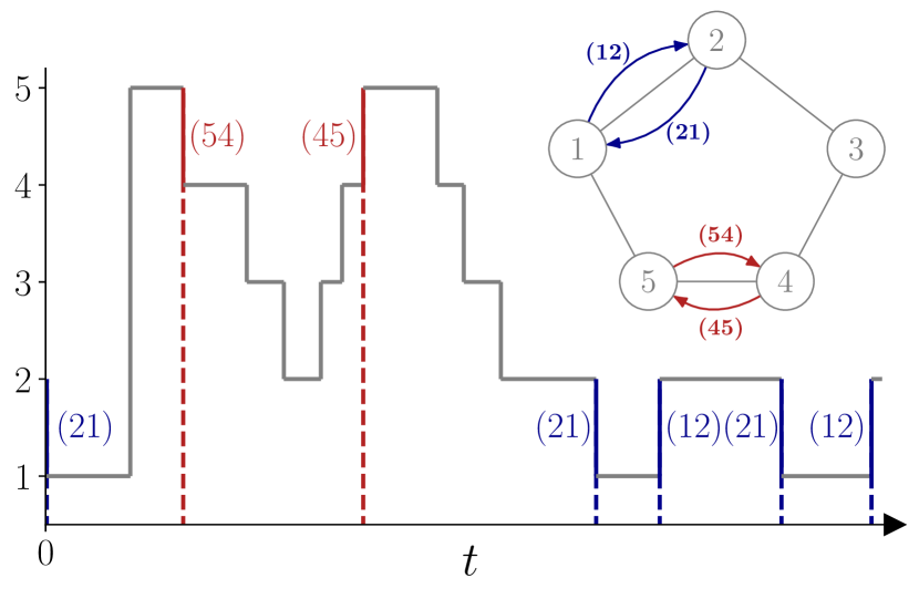
Figure 1: Observation of a partially accessible five-state Markov network with four resolved transitions. The resolved observer registers the transitions $(12),(21),$ $(45)$ and $(54)$ and the corresponding in-between waiting times.

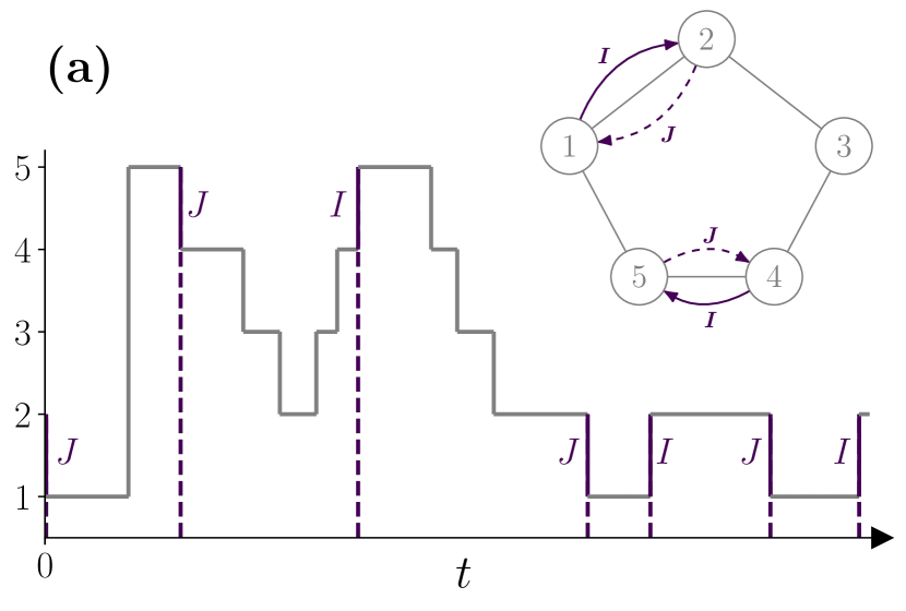
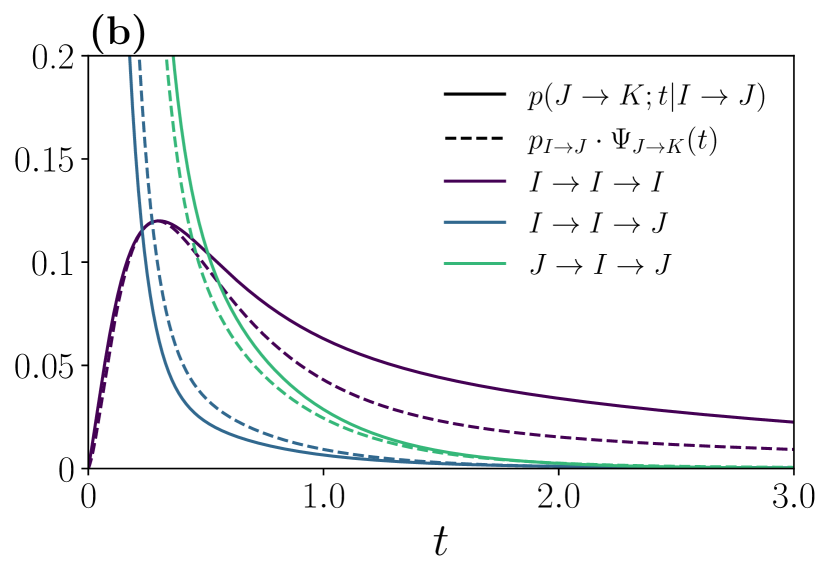
Figure 2: Observation of a partially accessible five-state Markov network with two blurred transitions. (a) The blurred observer registers transitions from classes $I$ and $J$ and the corresponding in-between waiting times but cannot resolve the individual transitions within a class. (b) Breakdown of the renewal property, i.e., Eq. (missing)14, for three out of eight possible sequences with three transitions. The required probabilities and waiting time distributions are calculated with an absorbing master equation for transition rates $k_{12}=0.4,k_{21}=8.9,k_{23}=4.2,$ $k_{32}=1.1,k_{34}=1.8,k_{43}=0.01,k_{45}=9.4,k_{54}=0.1,k_{51}=8.8$ and $k_{15}=0.6$.

In general, the emerging effective description of the network is non-Markovian because the described partial observation is not sufficient for determining the state of the underlying network. As a consequence, the corresponding waiting time distributions are typically non-exponential. However, directly after a registered transition, the state of the system is uniquely determined by this transition. For example, in Fig. missing1, observing $(12)$ implies that the state of the system directly after the transition is two. Therefore, the effective description remains Markovian at the corresponding time instances. From a conceptual point of view, these Markovian events [44, 45] can be interpreted as the renewal events of a semi-Markov process which describes the effective dynamics in the space of observable transitions [38]. Stated differently, an observed transition updates the semi-Markov state of the system by renewing the memory of the non-Markovian process with a Markovian event.

This updating of the semi-Markov state slices an observed trajectory into snippets starting and ending with an observed transition, i.e., a Markovian event. From an operational point of view, e.g., for the resolved observer, this slicing implies that waiting time distributions for transition sequences with more than two transitions factorize. For example, for the sequence $(ij)\to(kl)\to(mn)$ with in-between waiting times $t_{1}$ and $t_{2}$, we have

$$\psi_{(ij)\to(kl)\to(mn)}(t_{1},t_{2})=\psi_{(ij)\to(kl)}(t_{1})\psi_{(kl)\to(mn)}(t_{2}).$$ (7)

On the level of these trajectory snippets, a fluctuation theorem holds true which relates a single snippet to the completion of paths, especially of cycles [38, 39, 44]. Based on this fluctuation theorem, the entropy estimator

$$\braket{\hat{\sigma}}\equiv\sum_{(ij),(kl)}\int_{0}^{\infty}dt\pi_{ij}\psi_{(ij)\to(kl)}(t)\ln\frac{\psi_{(ij)\to(kl)}(t)}{\psi_{(\widetilde{kl})\to(\widetilde{ij})}(t)}$$ (8)

for the full entropy production $\braket{\sigma}$ of a partially accessible Markov network can be derived. In Eq. (missing)8, the summation includes all observed transitions, $(\widetilde{ij})=(ji)$ is the time-reversed transition of $(ij)$ and $\pi_{ij}=p^{s}_{i}k_{ij}$ is the rate for observing transition $(ij)$. This entropy estimator always provides a lower bound on the full entropy production, i.e., $\braket{\hat{\sigma}}\leq\braket{\sigma}$. Especially for unicyclic networks, the observation of transitions $(ij)$ and $(ji)$ along a single link recovers the full entropy production, i.e., $\braket{\hat{\sigma}}=\braket{\sigma}=j_{\mathcal{C}}\mathcal{A}_{\mathcal{C}}$, because

$$\int_{0}^{\infty}dt(\pi_{ij}\psi_{(ij)\to(ij)}(t)-\pi_{ji}\psi_{(ji)\to(ji)}(t))=j_{\mathcal{C}}$$ (9)

and

$$\ln\frac{\psi_{(ij)\to(ij)}(t)}{\psi_{(ji)\to(ji)}(t)}=\mathcal{A}_{\mathcal{C}}$$ (10)

hold true [38, 39].

III From resolved to blurred observations

We now assume that a second observer with finite resolution, whom we call “blurred observer” for later reference, also observes the $2M$ transitions of the underlying network. However, due to the finite resolution of his observation, this observer cannot distinguish between the $2M$ resolved transitions and instead observers $C$ blurred transitions with $2\leq C\leq M$. Stated differently, for the blurred observer, the resolved transitions are grouped into $C$ different effective transition classes $G,H,I,...$ with each transition belonging to one transition class. A concrete example in which the four observable transitions of the network in Fig. missing1 are blurred into two transition classes is shown in Fig. missing2 (a). For these transitions, the blurred observer registers only the corresponding transition class but cannot distinguish between individual transitions within each class. The conditioned probability for observing a specific transition $(ij)$ of transition class $I$ is given by

$$p(ij|I)=\frac{p^{s}_{i}k_{ij}}{\sum_{(kl)\in I}p^{s}_{k}k_{kl}}=\frac{\pi_{ij}}{\pi_{I}},$$ (11)

where $\pi_{I}$ is the rate for observing that a transition within $I$ happens and the summation includes all transitions within transition class $I$. Waiting time distributions for blurred transitions can be interpreted as an average over all waiting time distributions for resolved transitions belonging to the corresponding transition classes. Thus, these waiting time distribution can be calculated via

$$\Psi_{I\to J}(t)=\sum_{\mathclap{\begin{subarray}{c}(ij)\in I\\ (kl)\in J\end{subarray}}}p(ij|I)\psi_{(ij)\to(kl)}(t)$$ (12)

using the corresponding weight from Eq. (missing)11. Note that the interpretation of $\Psi_{I\to J}(t)$ is similar to the interpretation of the waiting time distributions for resolved transitions defined in Eq. (missing)7.

Although the waiting time distributions for blurred transitions can be interpreted analogously to the waiting time distributions for resolved transitions, their meaning on the level of the underlying Markov network is significantly different. Directly after a transition from class $I$, the state of the underlying system can be the final state of any transition within $I$. For example, for the observation scenario shown in Fig. missing2 (a), right after a registered transition from class $I$, the state of the system is either two or five. In general, after a blurred transition, the state of the system is not fully determined, i.e., the state of the system is determined up to $p(ij|I)$. Thus, the effective dynamics on the level of blurred observations is non-Markovian at any point in time.

From the perspective of the blurred observer, this breakdown of the renewal property leads to non-factorizing waiting time distributions, e.g., for the sequence $I\to J\to K$ with waiting times $t_{1}$ and $t_{2}$,

$$\Psi_{I\to J\to K}(t_{1},t_{2})\neq\Psi_{I\to J}(t_{1})\Psi_{J\to K}(t_{2}).$$ (13)

To illustrate Eq. (missing)13 with the two-transition waiting time distributions of the example in Fig. missing2 (a), we integrate both sides over $t_{1}$ leading to

$$p(J\to K;t|I\to J)\neq p_{I\to J}\Psi_{J\to K}(t_{2}),$$ (14)

where

$$p_{I\to J}=\int_{0}^{\infty}dt\Psi_{I\to J}(t)$$ (15)

is the probability to observe a transition from class $J$ after a transition from class $I$ irrespective of the in-between waiting time. For the three different sequences with three transitions shown in Fig. missing2 (b), the renewal property breaks down.

The mapping from resolved transitions to blurred transitions is a time-independent, unique and many-to-one coarse-graining scheme for an already effective description of a partially accessible Markov network by the resolved observer. In the space of observable transitions, this coarse-graining scheme corresponds to lumping effective transition states into effective compound transition states. Crucially, although this strategy is similar to conventional coarse-graining by state lumping [11, 7, 10, 15], the behavior of the resulting coarse-grained states under time-reversal is different. If we first apply the time-reversal operation for transitions and blur them into classes afterwards [35, 36, 38], these classes, in contrast to conventional lumped states, can be even, odd or neither be even nor odd under time-reversal. For thermodynamic consistency, we assume that for each transition class, the corresponding time-reversed one is observable. This means that we only consider transition classes which are either even or odd.

As an example, consider again the system shown in Fig. missing2. The transition classes $I=\{(12),(45)\}$ and $J=\{(21),(54)\}$ are odd transition classes, i.e., $\widetilde{I}=J$ and $\widetilde{J}=I$. In contrast, blurring the resolved transitions into $G=\{(12),(21)\}$ and $H=\{(45),(54)\}$ would result in even transition classes, i.e., $\widetilde{G}=G$ and $\widetilde{H}=H$. If the transitions were blurred into $K=\{(12),(21),(45)\}$ and $L=\{(54)\}$, the time-reversed transition classes $\widetilde{K}=\{(21),(12),(54)\}$ and $\widetilde{L}=\{(45)\}$ would not be observable.

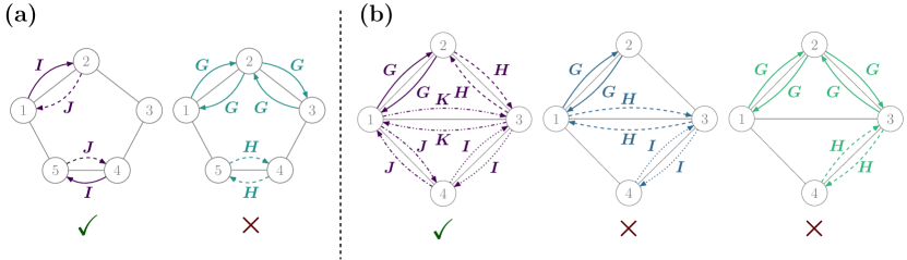
Figure 3: Illustration of the sufficient conditions for applying the entropy bound from Eq. (missing)20 to unicyclic networks (a) and multicyclic networks (b). (a) A transition preserving-observation of transition classes $I=\{(12),(45)\}$ and $J=\{(21),(54)\}$ (left) and a non transition-preserving observation of transition classes $G=\{(12),(21),(23),(32)\}$ and $H=\{(45),(54)\}$ (right) of a unicyclic five-state Markov network. (b) A transition-preserving observation of transition classes $G=\{(12),(21)\}$, $H=\{(23),(32)\}$, $I=\{(34),(43)\}$, $J=\{(41),(14)\}$ and $K=\{(13),(31)\}$ including all transitions of the network (left), a transition-preserving observation of transition classes $G=\{(12),(21)\}$, $H=\{(13),(31)\}$, $I=\{(34),(43)\}$ including not all transitions of the network (middle) and a non transition-preserving observation of transition classes $G=\{(12),(21),(23),(32)\}$ and $H=\{(34),(43)\}$ including not all transitions of the network (right) of a multicyclic four-state Markov network.

IV Estimation of entropy production

Extending the analogy between waiting time distributions of resolved transitions and blurred transitions to the entropy estimator $\braket{\hat{\sigma}}$ leads to a generalization of Eq. (missing)8 for blurred transitions given by

$$\braket{\hat{\sigma}_{\mathrm{BT}}}\equiv\sum_{I,J}\int_{0}^{\infty}dt\pi_{I}\Psi_{I\to J}(t)\ln\frac{\Psi_{I\to J}(t)}{\Psi_{\widetilde{J}\to\widetilde{I}}(t)}$$ (16)

where the summation includes all transition classes. Crucially, however, $\braket{\hat{\sigma}_{\mathrm{CG}}}$ is not a bound for $\braket{\sigma}$, i.e., $\braket{\hat{\sigma}_{\mathrm{CG}}}\nleq\braket{\sigma}$, because the entropy estimator for trajectory snippets is not applicable if the snippets are not Markovian, i.e., if there are no renewal events. To derive a waiting time based bound for blurred transitions, we start from Eq. (missing)16, insert the definition of the waiting time distributions from Eq. (missing)12 and apply the log-sum inequality from information theory [52] to obtain

$$\braket{\hat{\sigma}_{\mathrm{BT}}}\leq\sum_{I,J}\sum_{\mathclap{\begin{subarray}{c}(ij)\in I\\ (kl)\in J\end{subarray}}}\;\int_{0}^{\infty}dt\pi_{ij}\psi_{(ij)\to(kl)}(t)\ln\frac{p(ij|I)\psi_{(ij)\to(kl)}(t)}{p(\widetilde{kl}|\widetilde{J})\psi_{(\widetilde{kl})\to(\widetilde{ij})}(t)}$$ (17)

where the first summation includes transitions between all transition classes and the second summation includes all transitions within the corresponding class. Note that this double summation includes possible transitions between the same transition class, for example the blurred sequence $I\to I$ for the resolved observation of $(12)\to(45)$ in the example from Fig. missing2. By rearranging the terms of the double summation to separate the contributions from the waiting time distributions and the contributions from the probabilities, we arrive at the inequality

$$\braket{\hat{\sigma}_{\mathrm{BT}}}+\sum_{I,J}\pi_{I}p_{I\to J}\log\frac{\pi_{I}}{\pi_{\widetilde{J}}}\leq\sum_{I,J}\sum_{\mathclap{\begin{subarray}{c}(ij)\in I\\ (kl)\in J\end{subarray}}}\;\int_{0}^{\infty}dt\pi_{ij}\psi_{(ij)\to(kl)}(t)\ln\frac{\psi_{(ij)\to(kl)}(t)}{\psi_{(\widetilde{kl})\to(\widetilde{ij})}(t)}+\sum_{I,J}\sum_{\mathclap{\begin{subarray}{c}(ij)\in I\\ (kl)\in J\end{subarray}}}\pi_{ij}p_{(ij)\to(kl)}\ln\frac{\pi_{ij}}{\pi_{\widetilde{kl}}},$$ (18)

which we abbreviate as

$$\braket{\hat{\sigma}_{\mathrm{BT}}}+\braket{\hat{\sigma}_{\mathrm{TC}}}\leq\braket{\hat{\sigma}_{\mathrm{WT}}}+\braket{\hat{\sigma}_{\mathrm{RT}}}.$$ (19)

Here, we have first carried out the integration over all waiting times in the probability expression and have then rewritten the conditioned probabilities using Eq. (missing)11. The abbreviations $\braket{\hat{\sigma}_{\mathrm{TC}}}$, i.e., the transition class contribution, $\braket{\hat{\sigma}_{\mathrm{WT}}}$, i.e., the waiting time contribution, and $\braket{\hat{\sigma}_{\mathrm{RT}}}$, i.e., the resolved transition contribution, lead to Eq. (missing)19 as a compact representation of Eq. (missing)18.

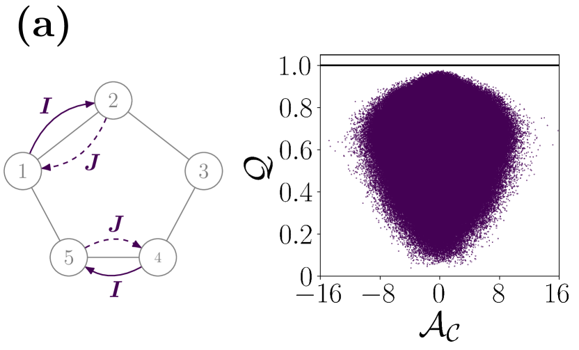
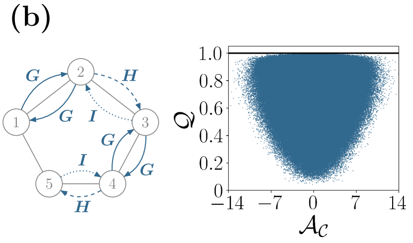
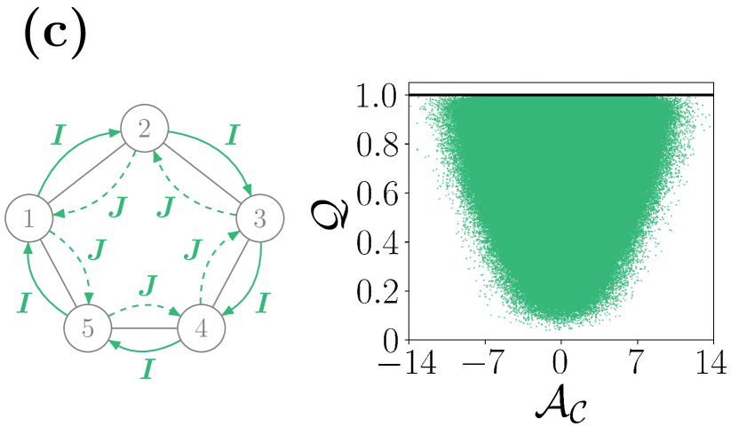
Figure 4: Quality of the entropy bound in Eq. (missing)20 for a unicyclic five-state Markov network as a function of the cycle affinity for three different observation scenarios. (a) Observation of the odd transition classes $I=\{(12),(45)\}$ and $J=\{(21),(54)\}$. The mean quality factor is given by $Q\simeq 0.66$. (b) Observation of the even transition class $G=\{(12),(21),(34),(43)\}$ and of the odd transition classes $H=\{(23),(45)\}$ and $I=\{(32),(54)\}$. The mean quality factor is given by $Q\simeq 0.77$. (c) Observation of the odd transition classes $I$ and $J$ including all forward and backward transitions, respectively. The mean quality factor is given by $Q\simeq 0.8$. Each scenario includes more than 4000000 network realizations with transition rates that are randomly drawn from uniform distributions between $0.1$ and $6$. All waiting time distributions are calculated with an absorbing master equation and Eq. (missing)12.

The operational value of this inequality is yet limited because, in general, neither $\braket{\hat{\sigma}_{\mathrm{WT}}}$ not $\braket{\hat{\sigma}_{\mathrm{RT}}}$ correspond to $\braket{\hat{\sigma}}$. Furthermore, both quantities are not accessible for the blurred observer. However, if the coarse-graining scheme for blurring transitions into transition classes fulfills two additional conditions detailed in the following paragraphs, Eq. (missing)19 reduces to the operationally accessible bound

$$\braket{\hat{\sigma}_{\mathrm{BT}}}+\braket{\hat{\sigma}_{\mathrm{TC}}}\leq 2\braket{\sigma}$$ (20)

for the full entropy production $\braket{\sigma}$.

First, if the waiting time distributions for all transitions that can be registered by the resolved observer are included in $\braket{\hat{\sigma}_{\mathrm{WT}}}$, we can equivalently replace the double summation for $\braket{\hat{\sigma}_{\mathrm{WT}}}$ in Eq. (missing)19 by a summation over all resolved transitions. Consequently, we have $\braket{\hat{\sigma}_{\mathrm{WT}}}=\braket{\hat{\sigma}}$ and thus

$$\braket{\hat{\sigma}_{\mathrm{BT}}}+\braket{\hat{\sigma}_{\mathrm{TC}}}\leq\braket{\hat{\sigma}}+\braket{\hat{\sigma}_{\mathrm{RT}}}$$ (21)

holds true. Since this condition implies that all resolved transitions are preserved in $\braket{\hat{\sigma}_{\mathrm{WT}}}$, we denote coarse-graining schemes fulfilling this condition as transition-preserving. A concrete example contrasting an observation with a transition-preserving coarse-graining scheme with an observation in which not all transitions of the resolved observer are preserved at the blurred level is shown in Fig. missing3 (a). As the transition classes $I$ and $J$ of the scheme on the left-hand side of Fig. missing3 (a) are odd under time-reversal, $\braket{\hat{\sigma}_{\mathrm{WT}}}$ includes waiting time distributions for the resolved transition pairs $(12)\to(45)$, $(45)\to(12)$ and their time-reversed partners implying $\braket{\hat{\sigma}_{\mathrm{WT}}}=\braket{\hat{\sigma}}$. For the even transition classes $G$ and $H$ of the scheme on the right-hand side of Fig. missing3 (a), however, $\braket{\hat{\sigma}_{\mathrm{WT}}}$ only includes waiting time distributions for the transition pairs $(23)\to(45)$, $(45)\to(12)$ and their time-reversed partners. The waiting time distributions for the transition pairs $(12)\to(23)$ and $(32)\to(21)$ visible to the resolved observer are not included in $\braket{\hat{\sigma}_{\mathrm{WT}}}$. Thus, for this observation scenario, $\braket{\hat{\sigma}_{\mathrm{WT}}}\neq\braket{\hat{\sigma}}$.

If the underlying Markov network is unicyclic, this condition is already sufficient for deducing the bound in Eq. (missing)20 from Eq. (missing)21. Since the entropy estimator $\braket{\hat{\sigma}}$ for transitions on the resolved level always recovers the full entropy production for unicyclic systems, i.e., $\braket{\hat{\sigma}}=\braket{\sigma}$, we have to bound $\braket{\hat{\sigma}_{\mathrm{RT}}}$. As the coarse-graining scheme is transition-preserving, we replace the double summation in $\braket{\hat{\sigma}_{\mathrm{RT}}}$ by a summation over all resolved transitions, plug in Eq. (missing)9 and note that

$$\braket{\hat{\sigma}_{\mathrm{RT}}}=j_{\mathcal{C}}\sum_{(ij),(kl)}\ln\frac{\pi_{ij}}{\pi_{\widetilde{kl}}}\leq j_{\mathcal{C}}\mathcal{A}_{\mathcal{C}}=\braket{\sigma}$$ (22)

holds true because we can always complete this summation to Eq. (missing)2 by adding $(\pi_{ij}-\pi_{ji})\ln\pi_{ij}/\pi_{ji}=j_{\mathcal{C}}\ln\pi_{ij}/\pi_{ji}\geq 0$ and canceling the steady state probabilities afterwards [48]. Thus, in this case, $\braket{\hat{\sigma}_{\mathrm{BT}}}+\braket{\hat{\sigma}_{\mathrm{TC}}}\leq 2\braket{\sigma}$.

Second, for multicyclic networks, we cannot bound $\braket{\hat{\sigma}_{\mathrm{RT}}}$ analogously to Eq. (missing)22 because the summation includes contributions from all cycles of the network. However, if all transitions of the underlying network are registered on the resolved level of observation, we have $\braket{\hat{\sigma}_{\mathrm{RT}}}=\braket{\sigma}$ by the definition of $\braket{\sigma}$ in Eq. (missing)1. Since $\braket{\hat{\sigma}}=\braket{\sigma}$ holds true for the observation of all network transitions as well[38], this additional condition leads to $\braket{\hat{\sigma}_{\mathrm{BT}}}+\braket{\hat{\sigma}_{\mathrm{TC}}}\leq 2\braket{\sigma}$. Therefore, we conclude that the bound in Eq. (missing)20 is applicable if the blurred observation is transition-preserving and additionally includes all transitions of the underlying network. A concrete example illustrating these two sufficient conditions for a multicyclic Markov network with four states is shown in Fig. missing3 (b). For the transition-preserving coarse-graining scheme on the left-hand side, the even transition classes $G,H,I,J$ and $K$ include all transitions of the underlying network implying $\braket{\hat{\sigma}_{\mathrm{WT}}}=\braket{\hat{\sigma}}=\braket{\sigma}$ and $\braket{\hat{\sigma}_{\mathrm{RT}}}=\braket{\sigma}$ which means that the bound is applicable. Although the scheme shown in the middle of Fig. missing3 (b) is also transition-preserving, the second condition is not fulfilled by this scheme because only six of ten transitions of the underlying network are observed. The coarse-graining scheme on the right-hand side of Fig. missing3 (b) fulfills neither the first condition nor the second condition because $\braket{\hat{\sigma}_{\mathrm{WT}}}$ only includes contributions from $(21)\to(34)$, $(21)\to(43)$, $(23)\to(34)$ and $(23)\to(43)$ and the corresponding time-reversed partners, which excludes in particular $(12)\to(23)$ and $(32)\to(21)$.

We remark that these two conditions are sufficient but not necessary for the bound in Eq. (missing)20 to hold true. For example, suppose that each transition class includes only one transition, i.e., no transitions are blurred. For this scenario, both sides of Eq. (missing)19 are equal, i.e., $\braket{\hat{\sigma}_{\mathrm{BT}}}=\braket{\hat{\sigma}_{\mathrm{WT}}}$ and $\braket{\hat{\sigma}_{\mathrm{TC}}}=\braket{\hat{\sigma}_{\mathrm{RT}}}$. Noting that such a coarse-graining scheme is transition-preserving, i.e., $\braket{\hat{\sigma}_{\mathrm{WT}}}=\braket{\hat{\sigma}}\leq\braket{\sigma}$, we can construct multicyclic systems for which Eq. (missing)20 is applicable even if the resolved observer does not register all network transitions.

Furthermore, we note that if the observation additionally contains all transitions of the network, the bound is saturated because $\braket{\hat{\sigma}_{\mathrm{BT}}}=\braket{\hat{\sigma}_{\mathrm{WT}}}=\braket{\sigma}$ and $\braket{\hat{\sigma}_{\mathrm{TC}}}=\braket{\hat{\sigma}_{\mathrm{RT}}}=\braket{\sigma}$ hold true. Clearly, this saturation implies that this bound recovers the full $\braket{\sigma}$ if all transitions of the network are observed and no transition is blurred.

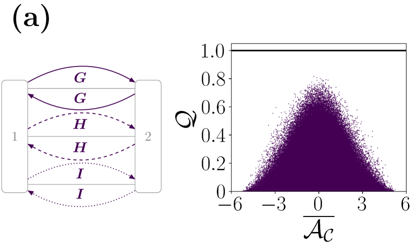
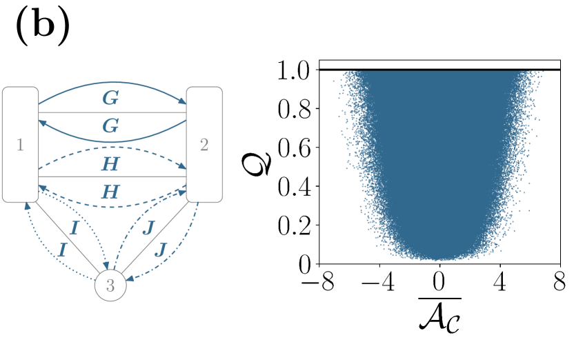
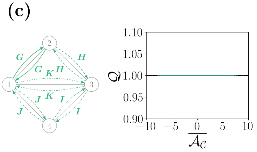
Figure 5: Quality of the entropy bound in Eq. (missing)20 for the observation of three multicyclic Markov network as a function of the average cycle affinity $\overline{\mathcal{A}_{\mathcal{C}}}$. For each link, the forward and backward transitions are blurred into the same transition class. (a) Observation of a three channel network with even transition classes $I,J$ and $K$. The mean quality factor is given by $Q\simeq 0.06$. (b) Observation of a three state network with two channels and even transition classes $H,I,J$ and $K$. The mean quality factor is given by $Q\simeq 0.67$. (c) Observation of a four state network with even transition classes $G,H,I,J$ and $K$. The mean quality factor is given by $Q\simeq 1.0$. Each observation includes more than 1300000 network realizations with transition rates that are randomly drawn from uniform distributions between $0.1$ and $6$. All waiting time distributions are calculated with an absorbing master equation and Eq. (missing)12.

V Illustration and numerical evidence

We illustrate our results and especially the class of systems for which Eq. (missing)19 reduces to the bound in Eq. (missing)20 with concrete observation scenarios for four different networks. To quantify the quality of the bound in Eq. (missing)20, we introduce the quality factor

$$\mathcal{Q}\equiv\frac{\braket{\hat{\sigma}_{\mathrm{CG}}}+\braket{\hat{\sigma}_{\mathrm{TC}}}}{2\braket{\sigma}}\leq 1.$$ (23)

V.1 Unicyclic networks

We consider three different scenarios for the observation of the unicyclic five-state network from Fig. missing2. For the observation scenario shown in Fig. missing4 (a), transitions of two different links are blurred into the odd transition classes $I$ and $J$. For randomly drawn transition rates, the scatter plot shows that $\mathcal{Q}<1$ for any drawn affinity $\mathcal{A}_{\mathcal{C}}$. Although the corresponding coarse-graining scheme is transition-preserving, the bound is never saturated. For this scenario, since only four of ten transitions of the underlying network are observed, the inequality in Eq. (missing)22 is, in the absence of additional symmetries, only saturated for a small set of rates which were not drawn in the simulation. In the modified scenario shown in Fig. missing4 (b), transitions of three different links are blurred into the even transition class $G$ and into the odd transition classes $H$ and $I$. Again, the scatter plot shows that $\mathcal{Q}\leq 1$ for all drawn cycle affinities. Compared to the scenario in (a), the quality of the bound increases because only the transitions $(51)$ and $(15)$ are not observed which implies that Eq. (missing)22 can be saturated for a larger set of rates. In the observation scenario shown in Fig. missing4 (c), all forward transitions are blurred into the odd transition class $I$ and all backward transitions are blurred into the odd transition class $J$. Since this coarse-graining scheme is transition-preserving and the observation includes all transitions of the network on the resolved level, the bound can be saturated for a large set of rates. Thus, as shown by the scatter plot, $\mathcal{Q}\leq 1$ for all drawn cycle affinities.

V.2 Multicyclic networks

We consider the observation of three different underlying multicyclic networks shown in Fig. missing5 (a)-(c). The networks in (a) and (b) have multiple channels for the transitions $(12)$ and $(21)$. For each network, all transitions are observed on the resolved level and the forward and backward transitions of each link or each channel are blurred into a single even transition class. Since this coarse-graining scheme is transition-preserving, the bound is applicable in all three considered scenarios. The corresponding scatter plots show that $\mathcal{Q}$ as a function of the average cycle affinity $\overline{\mathcal{A}_{\mathcal{C}}}=\sum_{\mathcal{C}_{i}}\mathcal{A}_{\mathcal{C}_{i}}/\#\;\mathrm{cycles}$, i.e., the sum of all cycle affinities divided by the number of cycles, is always smaller than one or equal to one.

The mean quality factors for the observation in Fig. missing5 (a), $Q\simeq 0.06$, in Fig. missing5 (b), $Q\simeq 0.67$, and in Fig. missing5 (c), $Q\simeq 1.0$, are significantly different indicating distinct quality regimes of the bound. Since, as previously mentioned, the bound is saturated if no transitions are blurred, i.e., if each registered transition determines the state of the underlying system completely, one possible explanation for this result is the different degree of non-Markovianity of the considered scenarios. In the scenario shown in Fig. missing5 (a), each registered blurred transition is a non-Markovian event because each pair of subsequent transition classes has two possible realizations on the level of resolved transitions. In contrast, in the scenario shown in Fig. missing5 (b), registering the blurred transitions $I\to J$ or $J\to I$ corresponds to a Markovian event because, due to the topology of the network, the only possible resolved transition sequences for $I\to J$ and $J\to I$ are $(13)\to(32)$ and $(23)\to(31)$, respectively. Generalizing this argumentation to the scenario in Fig. missing5 (c), the bound in Eq. (missing)20 is then saturated because for this network topology, each observed blurred transition corresponds to one unique transition registered by the resolved observer. Thus, each observed blurred transition is a Markovian event and the full $\braket{\sigma}$ is recovered in such a scenario where transitions of all links are observed without resolving their directionality.

VI Conclusion

In this paper, we have extended the transition-based description of partially accessible Markov networks to those with blurred transitions by introducing the concept of transition classes. To establish an effective description from the perspective of such a blurred observer, we have introduced waiting time distributions for transitions between transition classes. Based on these waiting time distributions, we have demonstrated that this effective description is in general non-Markovian, i.e., does not include any renewal event. As a consequence, the extant entropy estimator from Refs. [38, 44] defined for Markovian events is not applicable. As this result implies that the formulation of any direct waiting time based entropy estimator most likely will fail, we have proven a complementary bound based on the log-sum inequality which reduces to an operationally accessible entropy estimator for a broad class of systems fulfilling two additional conditions. Furthermore, we have illustrated the operational relevance of this class with various examples.

Future work could address the following issues. So far, the effective description is formulated for partially accessible Markov networks, which implies that its range of applicability is restricted to discrete systems. Generalizing the concept of transition classes to continuous degrees of freedom is a possible next step. This generalization could additionally lead to an entropy estimator for the continuous analogue of blurred transitions. Similarly, the description can potentially be generalized to systems which are not in a NESS, for example to systems with time-dependent driving. Our coarse-graining procedure leads to another open question. As state lumping is only one established coarse-graining scheme out of many, the extension of other schemes to the space of observable transitions might be possible as well. Assuming that these extensions lead to analogous bounds with a different range of validity, it might be possible to infer the realized coarse-graining in an observed systems based on the saturation or violation of the respective bounds.

References

- Sekimoto [2010] K. Sekimoto, Stochastic Energetics, Lecture Notes in Physics (Springer Berlin Heidelberg, Berlin, Heidelberg, 2010).
- Jarzynski [2011] C. Jarzynski, Equalities and Inequalities: Irreversibility and the Second Law of Thermodynamics at the Nanoscale, Annu. Rev. Condens. Matter Phys. 2, 329 (2011).
- Seifert [2012] U. Seifert, Stochastic thermodynamics, fluctuation theorems and molecular machines, Rep. Prog. Phys. 75, 126001 (2012).
- Schmiedl and Seifert [2007] T. Schmiedl and U. Seifert, Stochastic thermodynamics of chemical reaction networks, J. Chem. Phys. 126, 044101 (2007).
- Ge et al. [2012] H. Ge, M. Qian, and H. Qian, Stochastic theory of nonequilibrium steady states. part ii: Applications in chemical biophysics, Phys. Rep. 510, 87 (2012).
- Rao and Esposito [2016] R. Rao and M. Esposito, Nonequilibrium thermodynamics of chemical reaction networks: Wisdom from stochastic thermodynamics, Phys. Rev. X 6, 041064 (2016).
- Esposito [2012] M. Esposito, Stochastic thermodynamics under coarse graining, Phys. Rev. E 85, 041125 (2012).
- Mehl et al. [2012] J. Mehl, B. Lander, C. Bechinger, V. Blickle, and U. Seifert, Role of hidden slow degrees of freedom in the fluctuation theorem, Phys. Rev. Lett. 108, 220601 (2012).
- Uhl et al. [2018] M. Uhl, P. Pietzonka, and U. Seifert, Fluctuations of apparent entropy production in networks with hidden slow degrees of freedom, J. Stat. Mech. 2018 (2), 023203.
- Bo and Celani [2017] S. Bo and A. Celani, Multiple-scale stochastic processes: Decimation, averaging and beyond, Phys. Rep. 670, 1 (2017).
- Rahav and Jarzynski [2007] S. Rahav and C. Jarzynski, Fluctuation relations and coarse-graining, J. Stat. Mech. 2007 (09), P09012.
- Gomez-Marin et al. [2008] A. Gomez-Marin, J. M. R. Parrondo, and C. Van den Broeck, Lower bounds on dissipation upon coarse graining, Phys. Rev. E 78, 011107 (2008).
- Puglisi et al. [2010] A. Puglisi, S. Pigolotti, L. Rondoni, and A. Vulpiani, Entropy production and coarse graining in markov processes, J. Stat. Mech. 2010 (05), P05015.
- Bo and Celani [2014] S. Bo and A. Celani, Entropy production in stochastic systems with fast and slow time-scales, J. Stat. Phys. 154, 1325 (2014).
- Seiferth et al. [2020] D. Seiferth, P. Sollich, and S. Klumpp, Coarse graining of biochemical systems described by discrete stochastic dynamics, Phys. Rev. E 102, 062149 (2020).
- Roldán and Parrondo [2010] E. Roldán and J. M. R. Parrondo, Estimating dissipation from single stationary trajectories, Phys. Rev. Lett. 105, 150607 (2010).
- Roldán and Parrondo [2012] E. Roldán and J. M. R. Parrondo, Entropy production and Kullback-Leibler divergence between stationary trajectories of discrete systems, Phys. Rev. E 85, 031129 (2012).
- Shiraishi and Sagawa [2015] N. Shiraishi and T. Sagawa, Fluctuation theorem for partially masked nonequilibrium dynamics, Phys. Rev. E 91, 012130 (2015).
- Polettini and Esposito [2017] M. Polettini and M. Esposito, Effective Thermodynamics for a Marginal Observer, Phys. Rev. Lett. 119, 240601 (2017).
- Bisker et al. [2017] G. Bisker, M. Polettini, T. R. Gingrich, and J. M. Horowitz, Hierarchical bounds on entropy production inferred from partial information, J. Stat. Mech. 2017 (9), 093210.
- Barato and Seifert [2015] A. C. Barato and U. Seifert, Thermodynamic Uncertainty Relation for Biomolecular Processes, Phys. Rev. Lett. 114, 158101 (2015).
- Gingrich et al. [2016] T. R. Gingrich, J. M. Horowitz, N. Perunov, and J. L. England, Dissipation bounds all steady-state current fluctuations, Phys. Rev. Lett. 116, 120601 (2016).
- Pietzonka et al. [2016] P. Pietzonka, A. C. Barato, and U. Seifert, Universal bounds on current fluctuations, Phys. Rev. E 93, 052145 (2016).
- Marsland et al. [2019] R. Marsland, W. Cui, and J. M. Horowitz, The thermodynamic uncertainty relation in biochemical oscillations, J. R. Soc. Interface 16, 20190098 (2019).
- Horowitz and Gingrich [2020] J. M. Horowitz and T. R. Gingrich, Thermodynamic uncertainty relations constrain non-equilibrium fluctuations, Nat. Phys. 16, 15 (2020).
- Pietzonka and Coghi [2023] P. Pietzonka and F. Coghi, Thermodynamic cost for precision of general counting observables, arXiv:2305.15392 [cond-mat.stat-mech] (2023).
- Teza and Stella [2020] G. Teza and A. L. Stella, Exact coarse graining preserves entropy production out of equilibrium, Phys. Rev. Lett. 125, 110601 (2020).
- Ehrich [2021] J. Ehrich, Tightest bound on hidden entropy production from partially observed dynamics, J. Stat. Mech. 2021 (8), 083214.
- Skinner and Dunkel [2021a] D. J. Skinner and J. Dunkel, Improved bounds on entropy production in living systems, Proc. Natl. Acad. Sci. 118 (2021a).
- Elber [2020] R. Elber, Milestoning: An efficient approach for atomically detailed simulations of kinetics in biophysics, Annu. Rev. Biophys. 49, 69 (2020).
- Hartich and Godec [2021a] D. Hartich and A. Godec, Violation of local detailed balance despite a clear time-scale separation, arXiv:2111.14734 [cond-mat.stat-mech] (2021a).
- Berezhkovskii and Makarov [2019] A. M. Berezhkovskii and D. E. Makarov, On the forward/backward symmetry of transition path time distributions in nonequilibrium systems, J. Chem. Phys. 151, 065102 (2019).
- Martínez et al. [2019] I. A. Martínez, G. Bisker, J. M. Horowitz, and J. M. R. Parrondo, Inferring broken detailed balance in the absence of observable currents, Nat. Commun. 10, 3542 (2019).
- Hartich and Godec [2021b] D. Hartich and A. Godec, Emergent memory and kinetic hysteresis in strongly driven networks, Phys. Rev. X 11, 041047 (2021b).
- Hartich and Godec [2021c] D. Hartich and A. Godec, Comment on ”inferring broken detailed balance in the absence of observable currents”, arXiv:2111.14734 [cond-mat.stat-mech] (2021c).
- Bisker et al. [2021] G. Bisker, I. A. Martínez, J. M. Horowitz, and J. M. R. Parrondo, Comment on ”inferring broken detailed balance in the absence of observable currents”, arXiv:2202.02064 [cond-mat.stat-mech] (2021).
- Skinner and Dunkel [2021b] D. J. Skinner and J. Dunkel, Estimating Entropy Production from Waiting Time Distributions, Phys. Rev. Lett. 127, 198101 (2021b).
- van der Meer et al. [2022] J. van der Meer, B. Ertel, and U. Seifert, Thermodynamic inference in partially accessible markov networks: A unifying perspective from transition-based waiting time distributions, Phys. Rev. X 12, 031025 (2022).
- Harunari et al. [2022] P. E. Harunari, A. Dutta, M. Polettini, and E. Roldán, What to learn from a few visible transitions’ statistics?, Phys. Rev. X 12, 041026 (2022).
- Li and Kolomeisky [2013] X. Li and A. B. Kolomeisky, Mechanisms and topology determination of complex chemical and biological network systems from first-passage theoretical approach, J. Chem. Phys 139, 10.1063/1.4824392 (2013).
- Berezhkovskii and Makarov [2020] A. M. Berezhkovskii and D. E. Makarov, From Nonequilibrium Single-Molecule Trajectories to Underlying Dynamics, J. Phys. Chem. Lett. 11, 1682 (2020).
- Thorneywork et al. [2020] A. L. Thorneywork, J. Gladrow, Y. Qing, M. Rico-Pasto, F. Ritort, H. Bayley, A. B. Kolomeisky, and U. F. Keyser, Direct detection of molecular intermediates from first-passage times, Sci. Adv. 6, eaaz4642 (2020).
- Ertel et al. [2023] B. Ertel, J. van der Meer, and U. Seifert, Waiting time distributions in hybrid models of motor–bead assays: A concept and tool for inference, Int. J. Mol. Sci. 24, 7610 (2023).
- van der Meer et al. [2023] J. van der Meer, J. Degünther, and U. Seifert, Time-resolved statistics of snippets as general framework for model-free entropy estimators, Phys. Rev. Lett. 130, 257101 (2023).
- Degünther et al. [2023] J. Degünther, J. van der Meer, and U. Seifert, Fluctuating entropy production on the coarse-grained level: Inference and localization of irreversibility, arXiv:2309.07665 [cond-mat.stat-mech] (2023).
- Wang and Qian [2007] H. Wang and H. Qian, On detailed balance and reversibility of semi-markov processes and single-molecule enzyme kinetics, J. Math. Phys. 48, 013303 (2007).
- Maes et al. [2009] C. Maes, K. Netočný, and B. Wynants, Dynamical fluctuations for semi-markov processes, J. Phys. A: Math. Theor. 42, 365002 (2009).
- Ertel et al. [2022] B. Ertel, J. van der Meer, and U. Seifert, Operationally accessible uncertainty relations for thermodynamically consistent semi-markov processes, Phys. Rev. E 105, 044113 (2022).
- Godec and Makarov [2023] A. Godec and D. E. Makarov, Challenges in inferring the directionality of active molecular processes from single-molecule fluorescence resonance energy transfer trajectories, J. Phys. Chem. Lett. 14, 49 (2023).
- Hill [1989] T. L. Hill, Free Energy Transduction and Biochemical Cycle Kinetics (Springer New York, 1989).
- Jiang et al. [2004] D.-Q. Jiang, M. Qian, and M.-P. Qian, Mathematical Theory of Nonequilibrium Steady States (Springer Berlin Heidelberg, 2004).
- Cover and Thomas [2006] T. M. Cover and J. A. Thomas, Elements of Information Theory (Wiley Series in Telecommunications and Signal Processing) (Wiley-Interscience, USA, 2006).