Black-box Membership Inference Attacks against Fine-tuned Diffusion Models

Abstract

With the rapid advancement of diffusion-based image-generative models, the quality of generated images has become increasingly photorealistic. Moreover, with the release of high-quality pre-trained image-generative models, a growing number of users are downloading these pre-trained models to fine-tune them with downstream datasets for various image-generation tasks. However, employing such powerful pre-trained models in downstream tasks presents significant privacy leakage risks. In this paper, we propose the first reconstruction-based membership inference attack framework, tailored for recent diffusion models, and in the more stringent black-box access setting. Considering four distinct attack scenarios and three types of attacks, this framework is capable of targeting any popular conditional generator model, achieving high precision, evidenced by an impressive AUC of $0.95$.

1 Introduction

The recent developments in image-generative models have been remarkably swift, and many applications based on these models have appeared. Diffusion models [41, 18, 35, 40, 46, 53, 56, 44, 19, 54] have come to the forefront of the image generation. These models generate target images by progressive denoising a noisy sample from isotropic Gaussian distribution. In an effort to expedite the training of diffusion models and reduce training expenses, Stable Diffusion [44] was introduced. Leveraging the extensive and high-fidelity LAION-2B [48] dataset for training, the Stable Diffusion pre-trained checkpoint, available on HuggingFace, can be fine-tuned efficiently with just a few steps for effective deployment in downstream tasks. This model’s efficiency has spurred an increasing number of usages of Stable Diffusion.

At the same time, there has been a significant amount of research focused on the privacy concerns associated with these models [12, 20, 61, 6, 37, 34, 25, 14, 10, 13, 39, 49, 28]. Among them, membership inference attacks (MIAs) primarily investigate whether a given sample $x$ is included in the training set of a specific target model. While this line of research was traditionally directed toward classifier models [9, 21, 43, 45, 47, 51, 55, 60, 62], the popularity of diffusion models has led to the application of MIAs to examine potential abuses of privacy in their training datasets. Depending on the level of access to the target model, these attacks can be categorized into white-box attacks, gray-box attacks, and black-box attacks.

In a white-box attack scenario, attackers have access to all parameters of a model. Similar to membership inference attack targeting classifiers, attacks against diffusion models also utilize internal model information such as loss [6, 20, 34] or gradients [37] as attack features. Although white-box attacks can achieve high success rates, their limitation lies in the requirement for complete access to the target model’s information, which is often impractical in real-world scenarios. Compared with white-box attack, gray-box approaches do not require full access to the model’s parameters; instead, they only necessitate the intermediate outputs from the diffusion model during the denoising process to serve as features for inference [12, 14, 20, 25]. However, these attacks inevitably rely on the intermediate images generated during the model’s operation. In real-world scenarios, if a malicious model is trained using private or unsafe images, typically only the final output image is provided, with efforts made to conceal as many model details as possible. Therefore, the more practical scenarios would be black-box.

In the black-box setting, there are attacks for GANs [7, 17] and VAEs [17]. These are based on unconditional generative models and involve a highly stochastic generation process that requires extensive sampling for inference, which becomes inefficient when directly applied to diffusion models. The other black-box attacks [61, 63], although more tailored for diffusion models, focus on simulations and lack the necessary conditions to be used in realistic scenarios. We will discuss them in Section 2.4.

In this paper, we present a novel black-box attack framework fit for state-of-the-art image-generative models. The framework was built on a careful analysis of the objective function of the diffusion model as its theoretical foundation. It also incorporates four potential attack scenarios tailored for different settings of diffusion models. We demonstrate the efficacy of our attack using a Stable Diffusion model and further validate it on models fine-tuned with CelebA-Dialog [23], WIT [57], and MS COCO datasets [30].

Contributions:

• Many prior black-box attacks [17, 7, 61, 63, 34] on image-generative models are no longer practical for the current generation of models and attack scenarios. We propose a black-box membership inference attack framework that is deployable against any generative model by leveraging the model’s memorization of the training data.

• Consistent with the definition in Suya et al. [58], four attack scenarios are considered in which an attacker can perform an attack based on the query access as well as the quality of the initial auxiliary data, and three different inference models are used to determine the success rate of the attack, respectively.

• The efficacy of the attack is evaluated on the CelebA, WIT, and MS COCO datasets using Stable Diffusion as the representative target model. The attack’s impact is analyzed by considering various factors: image encoder selection, distance metrics, fine-tuning steps, inference step count, member set size, shadow model selection, and the elimination of fine-tuning in the captioning model.

Roadmap.

Section 2 reviews key works on denoising generative models and membership inference attacks, including their application against diffusion models. Section 3 introduces our reconstruction-based black-box attack on diffusion models, tailored to four levels of attacker knowledge. Section 4 describes our experimental setup, and Section 5 compares our attack’s effectiveness with existing methods and examines various influencing factors.  Section 6 shows that our attacks remain effective under common defenses.  Section 7 discusses some other research related to our work.  Section 8 concludes the paper, summarizing our main findings and contributions.

2 Background

2.1 Machine Learning

In general, we can classify a machine learning model into discriminative (classification) models and generative models.

2.1.1 Classification Models

In the context of classification model training, the objective is to map an input $x$ to a category $y$. The functional representation of the model can be expressed as $y=\mathcal{M}(x)$, where $x$ denotes the input image, and $y$ signifies the corresponding label. The loss in a classification model, which quantifies the discrepancy between the predicted and true labels, can be articulated as follows:

$$L(\theta)=\mathbb{E}_{x,y}\left[-\log(\mathcal{M}(x)_{y})\right]$$

where $\theta$ denotes the parameters of $\mathcal{M}$, $\mathcal{M}(x)$ denotes the model’s output probability distribution over the possible categories, and $\mathcal{M}(x)_{y}$ specifically denotes the probability assigned to the correct label $y$.

2.1.2 Generative Models

Generative models are designed to generate images $\hat{x}=\mathcal{M}(z)$, where $z$ is the randomness not provided by users by inherent to the server hosting the model.

Generative models include VAEs [24], GANs [15], and diffusion models [18]. Recently, diffusion models have gained significant traction. Building on the classical DDPM (Denoising Diffusion Probabilistic Models), a plethora of models, such as Imagen [46], DALL·E 3 [3], GLIDE [35], Stable Diffusion [44], have emerged and can generate high-quality images based on prompt information. In this paper, we focus on diffusion models.

Fundation of Diffusion Models.

The diffusion model can be conceptualized as a process where a noisy image is incrementally denoised to eventually yield a high-resolution image. Given an image $x_{0}$, the model initially imparts noise via $T$ forward (noisy-adding) processes. At timestep $t$, the noisy image $x_{t}$ can be represented as:

$$x_{t}=\sqrt{\bar{\alpha}_{t}}x_{0}+\sqrt{1-\bar{\alpha}_{t}}\epsilon_{t}$$ (1)

In this equation, $\bar{\alpha}_{t}=\prod_{i=1}^{t}\alpha_{i}$, where $\alpha_{i}$ is a predefined parameter that decreases incrementally within the interval $[0,1]$. The term $\epsilon_{t}$ is a random Gaussian noise derived using the reparameterization trick from multiple previous forward steps (more details in Appendix A).

The reverse process serves an objective opposite to that of the forward process. Starting from $\hat{x}_{T}=x_{T}$, upon obtaining the image $\hat{x}_{t}$ at timestep $t$, the reverse process aims to denoise it to retrieve the image $\hat{x}_{t-1}$. A neural network (i.e., U-Net) $\mathcal{U}_{\theta}$ is trained to predict the noise to be removed at each timestep. The loss function in the training process is defined as:

$$L_{t}(\theta)=\mathbb{E}_{x_{0},\epsilon_{t}}\left[\lVert\epsilon_{t}-\mathcal{U}_{\theta}(\sqrt{\bar{\alpha}_{t}}x_{0}+\sqrt{1-\bar{\alpha}_{t}}\epsilon_{t},t)\rVert^{2}_{2}\right]$$ (2)

Alternatively, this loss function can also be employed to train DDIM [54], which has a deterministic reverse process.

Prompt Guided Diffusion Models.

While various models [3, 40, 46, 35, 44] mentioned above are capable of generating high-quality images conditional on prompt information $p$, describe as $\hat{x}=M(z,p)$, further details can be found in Appendix B. Our experiments primarily utilize the current publicly available state-of-the-art model, Stable Diffusion [44]. Distinct from other diffusion generative models [35, 40, 46], Stable Diffusion uniquely conducts both the forward and reverse processes within the latent space. This approach offers advantages: the noise addition and removal processes operate over a smaller dimensionality, allowing for faster model training at lower computing costs. Additionally, within the latent space, the model can accommodate diverse prompt information to guide image generation. Importantly, Stable Diffusion is open-sourced and provides multiple high-quality pre-trained checkpoints online. This aligns well with the focus of our study on potential privacy concerns when fine-tuning pre-trained models for downstream tasks.

2.2 Membership Inference Attacks

Membership inference attacks (MIAs) primarily aim to determine whether a target data point $x$ is within the training dataset, often referred to as the member set, of a given target model. The motivation behind these attacks is twofold: to ensure that models are not trained in a manner that misappropriates data and to safeguard against potential privacy breaches. MIA’s underlying principle hinges on exploiting machine learning models’ overfitting and memorization properties. Discerning the model’s different reactions to member and non-member samples makes it feasible to infer the membership of the target point $x$.

Early MIAs predominantly target classification models and use the outputs from classifiers as the data to train their attack models [5, 26, 31, 47, 51, 9, 21, 45, 32, 33]. Shokri et al. [51] introduced a technique for training shadow models designed to use shadow models to approximate the target model’s behavior. By collecting information from these shadow models, such as predict vector or confidence scores, as well as labels such as members vs non-members, adversaries can subsequently train a binary classifier, acting as an attack model, to predict membership of $x$ based on the data derived from the querying $x$ on the target model.

Carlini et al. [5] suggest the use of confidence scores as attack features and the creation of two distributions, $\mathbb{D}_{\text{in}}$ and $\mathbb{D}_{\text{out}}$, based on the confidence scores of samples from the member and non-member sets, respectively. The distributions are then utilized to calculate the probability density function of a query data point $x$ in the member set and non-member set.

TABLE I: The symbols and represent an attacker’s fully authorized, partially authorized, and unauthorized data access, respectively. Symbols ✓ and ✗ denote the use and non-use of a technique, respectively. ‘HP’ stands for the model’s parameter settings. ‘TD’: training data used to train the target model. ‘IV’: model’s internal values, including loss and gradient. ‘IO’: internal outputs (noisy images). ‘TSC’: components (text and image) of the target sample. ‘SMs’: whether the attack employs shadow models.

	Method	HP	TD	MIV	IOs	TSC	SMs
White	Loss-based [20]						✗
	LiRA [6]						✓
	LOGAN [34]						✗
	GSA [37]						✓
Gray	SecMI [12]						✓
	PIA [25]						✗
	PFAMI [14]						✓
Black	GAN-Leaks [34]						✗
	Intuition-attack [61]						✗
	Distribution-attack [63]						✗
	Our Attack-I						✓
	Our Attack-II						✓
	Our Attack-III						✓
	Our Attack-IV						✓

MIAs against Diffusion Models

In the context of MIA against diffusion models, due to the structural differences between diffusion models and classification models, as well as the dissimilarities in their inputs and outputs, MIAs designed for classification models cannot be directly applied to diffusion models. The focus of research lies in how to construct features for MIA. We classify existing attacks against diffusion models as white-box, gray-box, and black-box, and introduce them separately. In white-box attacks, methods in this setting exploit the loss (derived from each timestep using Equation 2) and gradients (via backpropagation through the model). Gray-box attacks typically necessitate access to a model’s intermediate outputs but do not require any internal model information. For gray-box attacks targeting diffusion models, the model’s denoising trajectory, particularly the noisy images, is utilized as attack data. In contrast, black-box attacks operate without knowledge of the model’s internal mechanics or process outputs, relying solely on the final generated images for analysis. In Table I, we compare all existing attacks. Each type of attack’s details are deferred to Section 2.4.1 and Section 7.

2.3 Problem Formulation

2.3.1 Threat Model

Given the target sample $x$ and black-box access to the target image-generative model $\mathcal{M}$, the goal of the attacker is to determine whether $x$ was used to train $\mathcal{M}$. More specifically, we focus on the fine-tuning process, namely, we care about the privacy of the fine-tuning dataset of $\mathcal{M}$, and do not care about the pre-training dataset. We focus on fine-tuning because (1) the attacks will be similar for direct training, while the computational cost for experiments on fine-tuning MIA will be much smaller, and (2) the pertaining and fine-tuning paradigm is more popular with modern large models, and we will provide motivations for focusing on the fine-tuning process later.

We categorize the threat model into four scenarios with two dimensions, namely:

• Target Sample Component. One distinct property of the current image generator models is that there exists the flexibility to input text prompt or initial images to guide model generation. Two configurations for the attacker can be considered: First, the query data $x$ aligns with the training data as a text-image pair ($x=\langle T_{q},I_{q}\rangle$, where $T_{q}$ denotes the text component and $I_{q}$ denotes the corresponding image component). Second, the attacker only obtains a suspect image potentially revealing private information without a corresponding caption ($x=I_{q}$). As our focus here is MIAs on text-image generative models, the scenario where $x$ solely consists of text is not deemed practical and hence, is not discussed.

• Auxiliary Dataset. Similar to all other MIAs, we assume an auxiliary dataset $\mathbf{D}^{\prime}$ is available. It is used to train the shadow models $\mathcal{M}^{s}$ to mimic the behavior of the target model. We consider two scenarios for $\mathcal{D^{\prime}}$: $\mathbf{D}^{p}$ and $\mathbf{D}^{s}$, indicating whether the attacker has access to real samples used to fine-tune $\mathcal{M}$ or just samples from the same distribution.

Figure 1: The capability of current generative models to mimic artistic styles indicates their potential for creating derivatives of any artist’s work with adequate training data, thus leading to concerns about copyright and privacy implications.

2.3.2 Motivation

For a malicious publisher, training a generative model from scratch to produce malevolent images based on prompt information would entail significant computational costs. Therefore, the most efficient strategy for them would be to fine-tune a model that has already been pre-trained on a large-scale dataset. Given the full open-source nature of the Stable Diffusion [44], and the extensive availability of pre-trained models capable of generating photorealistic images from entities like CompVis and Stability AI, there has been an increasing trend of leveraging these pre-trained models for fine-tuning to specific downstream tasks. Furthermore, an increasing number of companies, such as Amazon, OctoML, and CoreWeave, are offering services in this domain. The data privacy issue during the training of these downstream tasks has not been explicitly studied. Our work seeks to uncover privacy leakage issues in this process and raise awareness of them.

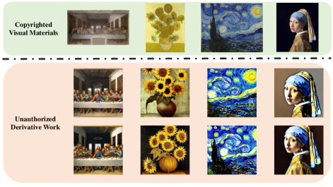
Our work can also serve as an auditing tool to address related to copyright and privacy infringements. For instance, if a malicious entity were to use a pre-trained Stable Diffusion model, and subsequently fine-tune it with artworks downloaded from the internet, it would be feasible to quickly train a generative model adept at replicating an artist’s unique style, leading to evident copyright violations. As depicted in Figure 1, for some renowned artworks that are already included in the model’s training set, high-quality replicated versions can now be generated. If malicious users intend to mimic an artist’s style and extensively fine-tune the model using the artist’s works, it is evident that such actions would pose significant infringements on the artist’s copyright.

2.4 Existing Solutions

2.4.1 Black-box MIA against Traditional Image-generatve Models

There are existing black-box MIAs targeting VAEs and GANs. They share a similar underlying idea, which is that if the target sample $x$ was used during training, the generated samples would be close to $x$. Monte-Carlo attack [17] invokes the target model many times to generate many samples first. Given $x$, it measures the number of generated samples within a specific radius. The more samples there are, the higher the likelihood that $x$ is part of the member set.

GAN-Leaks [7] employs a similar intuition and, instead of density in the Monte-Carlo attack [17]), roughly speaking, use the shortest distance of the generated samples from the target sample as the criteria. It also proposes another attack assuming an extra ability to optimize the noise input $z$ to the generator (which is not strictly the black-box setting; we will describe it and compare with it the evaluation) so it can reduce the number of generated samples. More formal details about these attacks are deferred to Appendix C.

2.4.2 Black-box MIA against Recent Diffusion Models

Matsumoto et al. [34] directly adopted the concept of GAN-Leaks [7] to diffusion models. However, as diffusion models are more complex, the attack is bottlenecked by the time required to sample a large number of samples.

Wu et al. [61] leveraged the intuition that the generated samples exhibit a higher degree of fidelity in replicating the training samples, and demonstrate greater alignment with their accompanying textual description. However, the authors only tested their attack on off-the-shelf models with explicitly known training sets. In the realistic setting where the training set is unknown (which is the purpose of MIAs), their attack cannot work.

Additionally, Zhang et al. [63] trained a classifier based on samples generated by the target model (labelled 1) and samples not used in training (labelled 0). The classifier can then determine whether the target sample was used in training. However, it needs to (1) know the non-training samples, and (2) ensure the two distributions (of generated samples and non-training samples) are different enough. Both conditions are not necessarily true in a realistic setting.

3 Methodology

Drawing inspiration from GAN-Leaks, our approach aims to determine the membership of query samples through similarity scores analysis. However, GAN-Leaks relies on Parzen window density estimation [38] to estimate the probability of model-generated query samples, which often results in non-stable probability estimates. We propose utilizing the intrinsic characteristics of diffusion models with formal proofs. Specifically, we leverage the training objective of diffusion models to more directly and intuitively represent the use of similarity scores as an attack feature for determining the membership of query samples.

Algorithm 1 High-level Overview of Our Attack.

1:Target sample $x$, target model $\mathcal{M}$, distance metrics $S(\cdot,\cdot)$, the image captioning model $\mathcal{C}$, and the image feature extractor $E$.

2:if $T_{q}$ $\notin$ $x$ then

3:     $T_{q}$ = $\mathcal{C}(I_{q})$ $\triangleright$ Synthesize the text for $\mathcal{M}$.

4:end if

5:for $i=1$ to $m$ do $\triangleright$ Perform $m$ repetitive queries.

6:     $I_{g}^{i}$ = $\mathcal{M}(T_{q})$

7:end for

8:$\mathcal{A}\left[\langle S(E(I_{g}),E(I_{q}^{i}))\rangle_{i=1}^{m}\right]$$\triangleright$ MIA results.

Moreover, our attack is tailored for modern diffusion models, which (compared to GANs and VAEs) have the capability of taking a text prompt and original image as input. Specifically, we utilize an image feature extractor and a captioning model, as detailed below.

Image Feature Extractor.

As we follow the high-level intuition of GAN-Leaks and use image similarities to determine membership, we need a metric to formally quantify this similarity. It has been observed that the semantic-level similarities are substantially more effective than pixel-level similarities [61]. So we utilize a pre-trained image encoder (i.e., DETR, BEiT, EfficientFormer, ViT, DeiT) to extract semantic information from the images.

Captioning Model.

As previously mentioned in Section 2.3.1, in some scenarios, the data record $x$ lacks the text component. Consequently, we resort to a captioning model to generate the corresponding text. For our experiments, we utilize BLIP2 [27] as the captioning model. To ensure that the generated textual descriptions closely match the style of the model’s training dataset, we also consider further use of query data and the auxiliary dataset to fine-tune the captioning model.

Attack Overview.

Algorithm 1 gives the high-level overview of our attack. The intuition is to compare the generated images with the target image and compute a similarity score used for MIAs (specific instantiations of $\mathcal{A}$ to be presented in Section 3.2). According to whether the text is available or not, we might need the captioning model to synthesize the text. Once the captioning is complete, we repeatedly query the victim model $m$ times to generate $m$ images. For each generated image, we calculate a similarity score relative to the query image. Finally, we return these as an $m$-dimensional similarity score to determine the target/query data’s membership.

Note that while the attack pipeline is perhaps straightforward, its intuition relies on the formal analysis of the diffusion models. In what follows, we first describe its theoretical foundation, and then instantiate it with different MIA paradigms based on the output score.

3.1 Theoretical Foundation

We aim to establish a theory demonstrating the distance between the query image $I_{q}$ and generated image $I_{g}$ can be used as a metric to infer the membership of $x$. We leverage the internal property of the diffusion model, which is inherently structured to optimize the log-likelihood: If $x$ is in the training set, its likelihood of being generated should be higher. However, due to the intractability of calculating log-likelihood in diffusion models, these models are designed to use the Evidence Lower Bound (ELBO) as an approximation of log-likelihood [18], as shown later in Equation 3. In Theorem 1, we first argue that ELBO of the diffusion model can be interpreted as a chain of generating images at any given timestep that approximates samples in the training set. Then, in Theorem 2, based on the loss function of the Stable Diffusion [44], we extend the result and demonstrate that this argument remains valid. Therefore, we can reasonably employ the similarity between the generated images and the query image as our attack. Note that GAN-Leaks [7] also shares this intuition of using similarity. However, it relies more on intuition and lacks a solid foundation, as the training of GANs is different (not a streamlined process as in diffusion models).

We elaborate on the theoretical foundation of our attack in the following detailed discussion.

Theorem 1.

Assuming we have a well-trained diffusion model $\hat{x}_{\theta}$, the high similarity scores between the query data $x$ and its generated image $\hat{x}_{\theta}(x_{t},t)$, the higher the probability of $\mathsf{Pr}\left[x\in\mathcal{D}_{m}|x,\theta\right]$.

$$\mathsf{Pr}\left[x\in\mathcal{D}_{m}|x,\theta\right]\propto-{\left\|x_{0}-\hat{x}_{\theta}(x_{t},t)\right\|^{2}_{2}}$$

where $\theta$ denotes the parameters of the model.

Proof.

Diffusion models employ the ELBO to approximate the log-likelihood $p(x)$ of the entire training dataset.

$$\log p({x}) \geq\mathbb{E}_{q(x_{1:T}|x_{0})}\left[\log\frac{p(x_{0:T})}{q(x_{1:T}|x_{0})}\right]$$

$$\cdots$$

$$=\underbrace{\mathbb{E}_{q(x_{1}|x_{0})}\left[\log p_{\theta}(x_{0}|x_{1})\right]}_{L_{0}}-\underbrace{\mathcal{D}_{KL}(q(x_{T}|x_{0})\|p(x_{T}))}_{L_{T}}$$

$$-\underbrace{\sum_{t=2}^{T}\mathbb{E}_{q}(x_{t}|x_{0})\left[\mathbf{D}_{KL}(q(x_{t-1}|x_{t},x_{0})\|p_{\theta}(x_{t-1}|x_{t}))\right]}_{L_{t-1}}$$ (3)

The primary focus of optimization is on $L_{t-1}$, as explicated in the original work [18]. The other terms are treated as constants and an independent decoders. Approximately, the objective function can be represented as

$$\min\mathbf{D}_{KL}(q(x_{t-1}|x_{t},x_{0})\;\|\;p_{\theta}(x_{t-1}|x_{t})).$$

Based on the assumption in DDPM [18], to elucidate further:

$$\underset{\theta}{\mathrm{arg\,min}}\,\mathbf{D}_{KL}(q(x_{t-1}|x_{t},x_{0})\;\|\;p_{\theta}(x_{t-1}|x_{t}))$$

$$= \underset{\theta}{\mathrm{arg\,min}}\mathbf{D}_{KL}(\mathbf{N}(\tilde{\mu}_{t}(x_{t},x_{0}),\sigma_{t}^{2}\textbf{I})\;\|\;\mathbf{N}(\mu_{\theta}(x_{t},t),\sigma_{t}^{2}\textbf{I}))$$

$$= \underset{\theta}{\mathrm{arg\,min}}\frac{1}{2\sigma_{t}^{2}}\left[\left\|\tilde{\mu}_{t}(x_{t},x_{0})-\mu_{\theta}(x_{t},t)\right\|^{2}_{2}\right]$$ (4)

In Equation 4, $q(x_{t-1}|x_{t},x_{0})$ represents the ground truth distribution of $x_{t-1}$ given $x_{t}$ and $x_{0}$, while $p_{\theta}(x_{t-1}|x_{t})$ denotes the predicted distribution of $x_{t-1}$ parameterized by $\theta$. The term $\tilde{\mu}_{t}(x_{t},x_{0})$ corresponds to the mean of the ground truth distribution $q(x_{t-1}|x_{t},x_{0})$, and $\mu_{\theta}(x_{t},t)$ corresponds to the mean of the predicted distribution $p_{\theta}(x_{t-1}|x_{t})$.

From Equation 11 and Equation 12 in Appendix A (which gives more details about diffusion models), we can rewrite Equation 4 as:

$$\underset{\theta}{\mathrm{arg\,min}}\frac{1}{2\sigma_{t}^{2}}\frac{\bar{\alpha}_{t-1}(1-\alpha_{t})^{2}}{(1-\bar{\alpha}_{t})^{2}}\left[\left\|x_{0}-\hat{x}_{\theta}(x_{t},t)\right\|^{2}_{2}\right]$$ (5)

Equation 5 can also be further developed by substituting and expressing $x_{0}$ using $x_{t}$ according to Equation 1, and by introducing $\epsilon_{t}$ as the targeted prediction of the diffusion model, aligning with the optimization objectives stated in both DDPM [18] and DDIM [54]. However, our aim is to demonstrate that the optimization goal of the diffusion model supports the use of similarity scores as an indicator for determining the membership of query data. Consequently, the objective function is merely reformulated in the form of Equation 5. Given that the likelihood of all training data should be higher than that of data not in the training set, and as inferred from Equation 3 and Equation 5, if a data point $x$ has a higher likelihood, the norm $\|x_{0}-\hat{x}_{\theta}(x_{t},t)\|$ at any timestep in the model should be smaller, indicating that the image generated by the model is closer to the original image. This can be expressed as:

$$\mathsf{Pr}\left[x\in\mathcal{D}_{m}|x,\theta\right]\propto-{\left\|x_{0}-\hat{x}_{\theta}(x_{t},t)\right\|^{2}_{2}}$$ (6)

∎

We have linked the probability of $x$ being a member to its similarity score with generated images in the unconditional diffusion model. Our next step is to prove this link persists in Stable Diffusion model.

Theorem 2.

In a well-trained Stable Diffusion model, $\hat{x}_{\theta}$, similarity scores remains a viable metric for assessing the membership of query data. A pre-trained encoder $\phi_{\theta}$ is used to convert input conditional prompt information $p$ into embeddings, which then guide image generation. This relationship can be expressed in the following mathematical formulation:

$$\mathsf{Pr}\left[x\in\mathcal{D}_{m}|x,\theta\right]\propto-{\left\|x_{0}-\hat{x}_{\theta}(z_{t},t,\phi_{\theta}(p))\right\|^{2}_{2}}$$

Proof.

In the original paper [44], the loss function of the Stable Diffusion model is described as follows:

$$L_{LDM}=\mathbb{E}_{\mathcal{E}(x),\epsilon\sim\mathcal{N}(0,1),t}\left[\|\epsilon_{t}-\mathcal{U}_{\theta}(z_{t},t,\phi_{\theta}(p))\|^{2}_{2}\right]$$

The latent code $z_{t}$ is of a much smaller dimension than that of the original image. The denoising network $\mathcal{U}_{\theta}$ predicts the noise at timestep $t$ based on $z_{t}$ and the embedding generated by $\phi_{\theta}$, which takes $p$ as its input. Given that the forward process of the Stable Diffusion [44] is fixed, Equation 1 remains applicable. Therefore, by substituting in the expression $\epsilon_{t}=\frac{x_{t}-\sqrt{\bar{\alpha_{t}}}x_{0}}{\sqrt{1-\bar{\alpha}_{t}}}$ and discarding other weight terms, we can rederive the loss function of the Stable Diffusion model as:

$$L_{LDM}=\mathbb{E}_{\mathcal{E}(x),t}\left[\|x_{0}-\hat{x}_{\theta}(z_{t},t,\phi_{\theta}(p))\|^{2}_{2}\right]$$ (7)

As seen from Equation 7, Stable Diffusion is essentially trained to optimize image predictions at any given timestep to closely approximate the original $x_{0}$. For the Stable Diffusion model, we can still distinguish between member samples and non-member samples by the similarity scores $||x_{0}-\hat{x}_{\theta}(z_{t},t,\phi_{\theta}(p))||^{2}_{2}$, which is expressed as:

$$\mathsf{Pr}\left[x\in\mathcal{D}_{m}|x,\theta\right]\propto-{\left\|x_{0}-\hat{x}_{\theta}(z_{t},t,\phi_{\theta}(p))\right\|^{2}_{2}}$$ (8)

∎

In Equation 8, we prove that under the attack situation, when the model has pre-trained parameters $\theta$, the probability of $x$ being a member set sample is inversely proportional to

$$\left\|x_{0}-\hat{x}_{\theta}(x_{t},t,\phi_{\theta}(p))\right\|^{2}_{2}.$$

Since this representation quantifies the distance between the predicted original image and the actual ground truth during training, we can denote the image generated by model as $I_{g}$ (which also corresponds to $\hat{x}$ in Section 2.1.2). The similarity score between $I_{g}$ and $I_{q}$ from the query data $x$ can be represented as $S(I_{q},I_{g})$. Here, $S$ is a distance metric (i.e., Cosine similarity, $\ell_{1}$ or $\ell_{2}$ distance, or Hamming distance). Given that a higher similarity score indicates a higher probability of the data being a training sample, inference model can be formulated accordingly.

$$\mathcal{A}_{base}(x,\theta)=\mathbbm{1}\left\{S(I_{q},I_{g})\geq\tau\right\}$$ (9)

The basic inference model relies on computing the similarity between $I_{g}$ and $I_{q}$. If the similarity score $S(I_{q},I_{g})$ exceeds a certain threshold, the inference model will determine that the data record $x$, to which $I_{q}$ belongs, originates from the member set.

3.2 Instantiations

Utilizing the scores obtained from Algorithm 1, we instantiate three different types of MIAs according to Section 2.2. In our evaluation, we try all three of them, and observe the last one is usually the most effective one.

Threshold-based Membership Inference Attack.

The threshold-based MIA takes the similarity scores, apply a statistical function $f$ to it, and then decide membership if the result is above a pre-defined threshold $\tau$, i.e.,

$$\displaystyle f\left[\left\langle S\left(E(I_{q}),E(I_{g}^{i})\right)\right\rangle_{i=1}^{m}\right]\geq\tau$$ (10)

Figure 2: AUC results on three datasets and four attack scenarios comparing five different image feature extractors.

Distribution-based Membership Inference Attack.

Following the work by Carlini et al. [5], we know we can also use the likelihood ratio attack against diffusion models. In our analysis, we leverage similarity scores derived from shadow models to delineate two distinct distributions: $\mathbb{Q}_{in}$ and $\mathbb{Q}_{out}$. Specifically: For $\mathbb{Q}_{in}$, consider query image $I_{q}$ that belong to the member set $\mathbf{D}_{m}$. We then define $\mathbb{Q}_{in}$ as

$$\mathbb{Q}_{in} =\left\{f\left[\left\langle S\left(E(I_{q}),E(I_{g}^{i})\right)\right\rangle_{i=1}^{m}\right]\;\bigg{|}\;I_{q}\in\mathbf{D}_{m}\right\}.$$

Similarly, for $\mathbb{Q}_{out}$, when query image $I_{q}$ are part of the non-member set $\mathbf{D}_{nm}$, we have

$$\mathbb{Q}_{out} =\left\{f\left[\left\langle S\left(E(I_{q}),E(I_{g}^{i})\right)\right\rangle_{i=1}^{m}\right]\;\bigg{|}\;I_{q}\in\mathbf{D}_{nm}\right\}.$$

For target query point $x$, membership inference can be deduced by assessing:

$$\mathsf{Pr}\left[f\left[\left\langle S\left(E(I_{q}),E(I_{g}^{i})\right)\right\rangle_{i=1}^{m}\right]\bigg{|}\mathbb{Q}_{in}\right]$$

and

$$\mathsf{Pr}\left[f\left[\left\langle S\left(E(I_{q}),E(I_{g}^{i})\right)\right\rangle_{i=1}^{m}\right]\bigg{|}\mathbb{Q}_{out}\right]$$

Classifier-based Membership Inference Attack.

Given that the obtained similarity score is represented as a high dimensional vector, the classifier-based MIA feeds $f\left[\left\langle S\left(E(I_{q}),E(I_{g})\right)\right\rangle_{i=1}^{m}\right]$ directly into a classifier (we use a multilayer perceptron in our evaluation). This approach aligns with the methods of Shokri et al. [51], leveraging the machine learning model as the inference model to execute the attack.

In evaluation, although we can use different functions of $f$, we observe a simple $f$ that takes the mean of all $m$ similarity scores performs pretty stable, so we just use the mean function for all three MIAs throughout the evaluation.

Figure 3: Composition of target points using solely $I_{q}$ with text caption generation by BLIP2 [27] captioning model, followed by image generation denoted as $I_{g}$ using the fine-tuned Stable Diffusion model.

4 Experiment Setup

4.1 Datasets

In this study, we primarily employ the MS COCO [30], CelebA-Dialog [23], and WIT datasets [57] for evaluation. MS COCO is widely used for training and testing various text-to-image models. The CelebA-Dialog dataset, with its extensive facial data and descriptions, aligns well with our interest in sensitive data descriptions. Meanwhile, the WIT dataset, curated from web scraping Wikipedia for images and their associated text descriptions, offers a diverse range of images and distinct textual styles, serving as an excellent benchmark for assessing model robustness.

MS COCO

is a large-scale dataset featuring a diverse array of images, each accompanied by five similar captions, amounting to a total of over $330$k images. The MS COCO dataset [30] has been extensively utilized in various image generation models, including experiments on DALL·E 2 [40], Imagen [46], GLIDE [35], and VQ-Diffusion [16]. In this work, we randomly selected $50$k images along with their corresponding captions to do the experiments. Each image is paired with a single caption to fine-tune the model.

CelebA-Dialog

is an extensive visual-language collection of facial data. Each facial image is meticulously annotated and encompasses over $10,000$ distinct entities. Given that each face image is associated with multiple labels and a detailed caption, the dataset is suitable for a range of tasks, including text-based facial generation, manipulation, and face image captioning. Facial information has consistently been regarded as private; hence, utilizing CelebA-Dialog [23] in this study aligns with our objective of detecting malicious users fine-tuning the Stable Diffusion model [44] for simulating genuine face generation.

WIT

is a vast image-text dataset encompassing a diverse range of languages and styles of images and textual descriptions. It boasts $37.6$ million image-text pairs and $11.5$ million images, showcasing remarkable diversity. We leverage this dataset specifically to evaluate the robustness of our attack in handling such heterogeneous data.

4.2 Evaluation Metrics

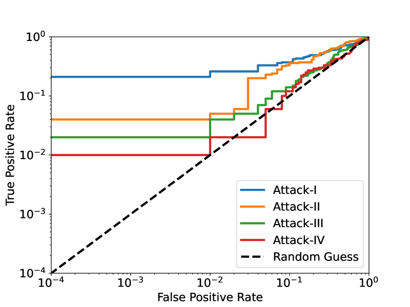
To systematically evaluate the efficacy of our proposed attack, we opted for multiple evaluation metrics as performance indicators. Similar to other comparable attacks [12, 20, 34, 25, 61, 6, 5], we will employ Attack Success Rate (ASR), Area Under the Curve (AUC), and True Positive Rate (TPR) at low False Positive Rate (FPR) as our evaluation metrics.

We opted to use Stable Diffusion v$1$-$5$ checkpoints as our pre-trained models. All experiments were carried out using two Nvidia A100 GPUs, and each fine-tuning of the model required an average of three days.

4.3 Competitors

For our evaluation, we first compare our work with existing black-box attacks on diffusion models [34, 14]. For our attack, based on the categorization provided in Section 2.3.1, the attacker will obtain information of two distinct dimensions, leading to four different scenarios. We call them Attack-I to Attack-IV. Below we introduce them in more detail.

Matsumoto et al. [34]

employed the full-black attack framework from GAN-Leaks.

Zhang et al. [63]

utilized a novel attack strategy involving a pre-trained ResNet18 as a feature extractor. This approach focuses on discriminating between the target model’s generated image distribution and a hold-out dataset, thereby fine-tuning ResNet18 to become a binary classification model.

Attack-I $(x=\langle T_{q},I_{q}\rangle,\mathcal{D^{\prime}}\cap\mathcal{D}_{m}\neq\emptyset)$

In this attack scenario, we assume the attacker has access to partial samples from the actual training (fine-tuning) set of the target model (attacker’s auxiliary data $\mathcal{D^{\prime}}$ overlaps with the fine-tuning data $\mathcal{D}_{m}$). Furthermore, $x$ includes both the image and the corresponding text (caption information). An attacker can directly utilize $T_{q}$ to obtain $I_{g}$, then employ the similarity between $I_{g}$ and $I_{q}$ to ascertain the membership of $x$.

Attack-II $(x=I_{q},\mathcal{D^{\prime}}\cap\mathcal{D}_{m}\neq\emptyset)$

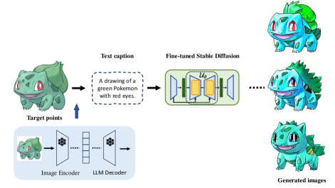
In this scenario, the attacker does not possess a conditional prompt that can be directly fed into the target model. As illustrated in Figure 3, the attack scenario necessitates the use of an image captioning model to produce a caption for $I_{q}$. This caption is subsequently used as the input for $\mathcal{M}$. The process culminates in the computation of similarity between the query image $I_{q}$ and the image generated by $\mathcal{M}$.

Attack-III $(x=\langle T_{q},I_{q}\rangle,\mathcal{D^{\prime}}\cap\mathcal{D}_{m}=\emptyset)$

is similar to the first scenario (the difference is the attacker’s auxiliary dataset does not intersect with the target training dataset). The attack (as shown in Algorithm 1) is the same, but we expect a lower effectiveness.

Attack-IV $(x=I_{q},\mathcal{D^{\prime}}\cap\mathcal{D}_{m}=\emptyset)$

is similar to the second scenario.

Figure 4: Relationship between epoch progression and attack success rates in  Attack-I, Attack-II, Attack-III, and Attack-IV, indicating increasing memorization within image generation models over fine-tuning epochs.

5 Experiments Evaluation

5.1 Comparison with Baselines

TABLE II: Accuracy comparison between the attacks by Zhang et al. [63] and Matsumoto et al. [34] versus our methods: Attack-I, Attack-II, Attack-III, and Attack-IV, illustrating the distinct success rates.

Attack type	CelebA-Dialog
	ASR	AUC	TPR@FPR=1%
Matsumoto et al. [34]	$0.52$	$0.50$	$0.01$
Zhang et al. [63]	$0.51$	$0.49$	$0.01$
Attack-I	$0.85$	$0.93$	$0.53$
Attack-II	$0.88$	$0.93$	$0.60$
Attack-III	$0.87$	$0.94$	$0.54$
Attack-IV	$0.87$	$0.93$	$0.57$

Results are shown in Table II. We ensure consistency in simulating real-world scenarios, wherein the number of images that a malicious publisher can sample from the target generator is limited. Under the constraint of limited sample size, we observe that the accuracy of both baseline attacks nearly equates to random guessing. We conjecture that this is due to their reliance on a large number of synthesis images for decision-making. Specifically, Zhang et al. [63]’s approach requires learning the distributional differences between generated image samples and non-member samples using ResNet18, based on a substantial volume of images sampled from the target model, and subsequently applying this knowledge to assess the input query data. However, such an attack premise falters in realistic scenarios where a malicious model publisher restricts the number of images a user can obtain from the model, preventing attackers from sampling a large volume of images to conduct the attack. Under such constraints, the effectiveness of attacks by Zhang et al. [63] and others is inevitably compromised, as the insufficient sample size hampers the ability to accurately discern the differences between the two data distributions. Similarly, the approach by Matsumoto et al. [34] encounters a hurdle; in scenarios of limited generative sample availability, it becomes challenging to find a suitable reconstruction counterpart and calculate its distance from the original data record. Consequently, these methods fail to achieve high attack success rates under sample-restricted conditions. In contrast, the four attack methods we propose still attain a high success rate despite the limited number of generative samples. This is attributed to our attacks being based on the similarity scores as proposed in Section 3.1, which, while influenced by the quality of the model’s generated images, is not hindered by the quantity of these images.

Threshold attack against CelebA

Threshold attack against WIT

Threshold attack against MS COCO

Distribution attack against CelebA

Distribution attack against WIT

Distribution attack against MS COCO

Classifier attack against CelebA

Classifier attack against WIT

Classifier attack against MS COCO

Figure 6: Experimental evaluation of three attack types (threshold-based, distribution-based, classifier-based) across three datasets in four scenarios ( Attack-I,  Attack-II,  Attack-III,  Attack-IV) highlighting Cosine similarity’s superior and stable performance across all metrics and attack types.

5.2 Different Image Encoder

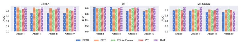
As our attack is a similarity scores-based attack, and we measure the distance between the query image $I_{q}$ and the image $I_{g}$ generated by the target model using the embeddings $E(I_{g})$ and $E(I_{q})$. However, due to the multitude of high-performance image encoder models, each with its unique pre-trained dataset and model architecture, We employed DETR [4], BEiT [2], EfficientFormer [29], ViT [11], and DeiT [59] five distinct image feature extractors to generate image embeddings, with the aim of observing the impact of various image features on the success rate of attacks. Furthermore, the extractor yielding the highest success rate will be selected as the default image feature extractor for subsequent experiments.

As depicted in Figure 2, our five image feature extractors excel across four different attack scenarios within the classifier-based attack domain. Each maintains an attack accuracy exceeding $70\%$, underscoring the robustness of our attack framework across different feature extractors. Notably, the implementation of DeiT [59] as the feature extraction model yielded a marginally higher and more consistent success rate compared to the other image encoders. Therefore, we selected DeiT as the default image encoder for future experimental investigations.

A more comprehensive comparison including threshold-based and distribution-based of these five image encoders is presented in Appendix F.

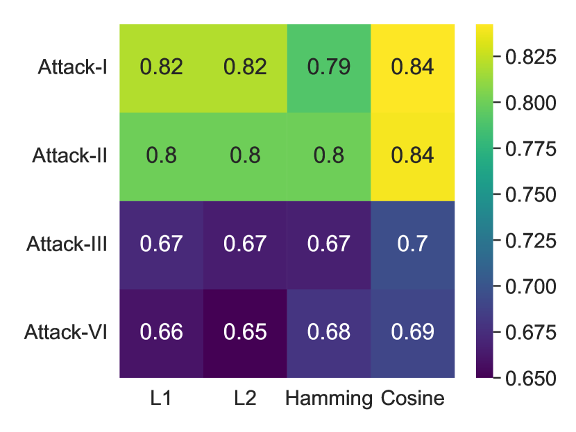
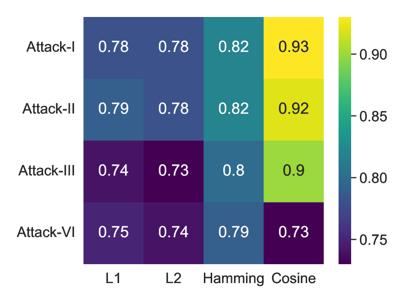
5.3 Different Distance Metrics

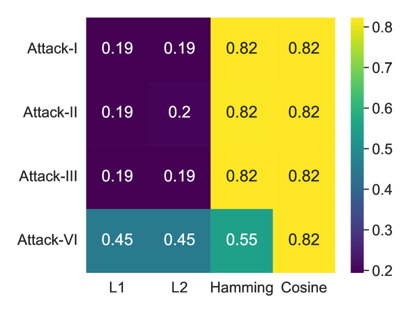
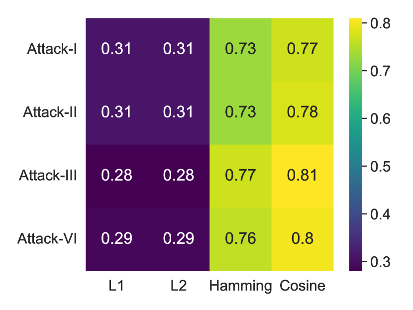
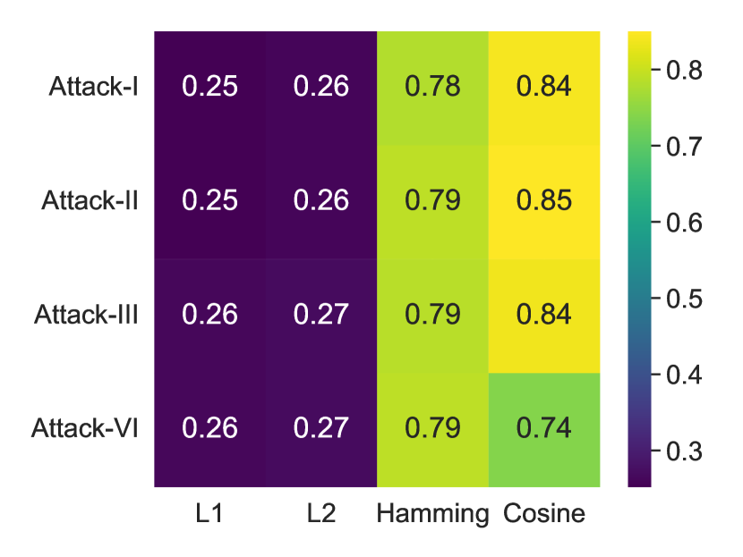
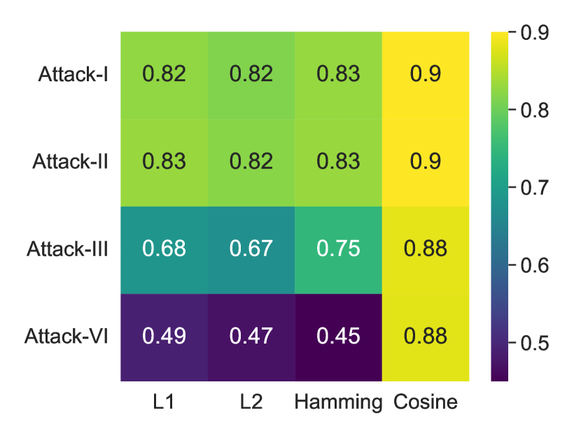
In the previous section, we picked DeiT [59] as the most stable and efficient image feature extractor. However, our attack framework also necessitates a reliable and consistent similarity metric to compute the closeness between embeddings. We conducted systematic and extensive experiments, and as demonstrated in Figure 6, we thoroughly assessed various attack scenarios and types across all datasets to test their effects on Cosine similarity, $\ell_{1}$ distance, $\ell_{2}$ distance, and Hamming distance.

From Figure 6, it is evident that using Cosine similarity as the distance metric yields optimal results for the computed distance vector, regardless of the attack scenario and type employed. We hypothesize that this phenomenon can be attributed to the focal point of our computation: the image embedding vectors generated by the encoder for both $I_{q}$ and $I_{g}$. Cosine similarity is inherently adept at measuring the similarity between two vectors. In contrast, $\ell_{1}$ and $\ell_{2}$ norms are more suitable for quantifying pixel-level discrepancies between $I_{q}$ and $I_{g}$, making them less efficient for evaluating the distance between two vectors.

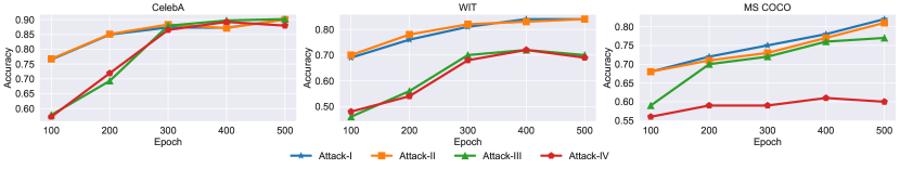
5.4 Impact of Fine-tuning Steps

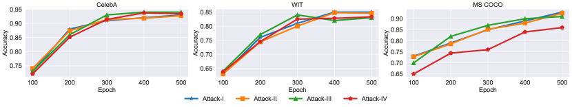
We then investigated the influence of the number of fine-tuning steps on the success rate of attacks. Evaluations were conducted at intervals of $100$ epochs, ranging from $100$ to $500$ epochs, to measure the attack success rate. As the model’s memorization of the training data can be equated to overfitting effects, it is anticipated that with an increased number of fine-tuning steps, the model increasingly exhibits a tendency towards overfitting and enhanced memorization of the training samples. Consequently, when querying the model with member set samples compared to non-member samples, a more distinct similarity discrepancy should be observed.

In Figure 4, we present the results of the classifier-based attacks under four attack scenarios: Attack-I, Attack-II, Attack-III, and Attack-IV. The outcomes indicate that Attack-I and Attack-III achieve higher success rates compared to the other two scenarios. This can be attributed to the fact that when utilizing the query data sample $x$, it inherently comprises the text caption $T_{q}$. As a result, neither Attack-I nor Attack-III require the employment of a caption model to generate corresponding text descriptions based on $I_{q}$. This circumvents the introduction of extra biases that might cause discrepancies between the model-generated images and $I_{q}$ itself.

We have also included the results for threshold-based and distribution-based attacks under these four scenarios in the Appendix D for reference.

5.5 Impact of Number of Inference Step

Figure 7: Model fine-tuning with CelebA-Dialog and image synthesis at inference steps of $30$, $50$, $100$, and $200$.

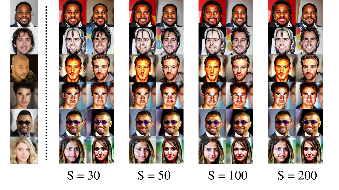
The quality of images generated by current diffusion models, including the Stable Diffusion [44] presented in our work, is influenced not only by the number of fine-tuning steps but also significantly by the number of inference steps. These models predominantly utilize Denoising Diffusion Implicit Models [54] as their sampling method. The Fréchet Inception Distance is able to shift significantly from $13.36$ to $4.04$ when varying the sampling steps from $10$ to $1000$. This dramatic change highlights the capability of a higher number of inference steps to produce images of superior quality. Given that the foundation of our attack relies on the distance between generated and original images, we posit that an increased number of inference steps, which results in images closely resembling the original and of better quality, would correspondingly enhance the attack’s success rate.

TABLE III: Alignment with DDIM [54] denoting ‘S’ as inference steps; experimentation under Attack-III scenario measuring FID at varying inference step counts.

S	Threshold-based			Distribution-based			Classifier-based			FID
	ASR	AUC	T@F=1%	ASR	AUC	T@F=1%	ASR	AUC	T@F=1%
30	$0.75$	$0.8225$	$0.30$	$0.76$	$0.8816$	$0.50$	$0.865$	$0.93$	$0.54$	$8.77$
50	$0.765$	$0.8146$	$0.25$	$0.77$	$0.8920$	$0.37$	$0.85$	$0.93$	$0.58$	$7.835$
100	$0.74$	$0.8172$	$0.26$	$0.745$	$0.8818$	$0.40$	$0.855$	$0.94$	$0.61$	$7.527$
200	$0.745$	$0.8125$	$0.39$	$0.74$	$0.8869$	$0.49$	$0.87$	$0.94$	$0.58$	$7.472$

Figure 8: Attack nomenclature and performance trends:‘T’ for threshold-based, ‘D’ for distribution-based, and ‘C’ for classifier-based attacks, with accuracy inversely related to training set size.

As illustrated in Table III, the variations in attack accuracy are not immediately pronounced. However, upon a broader examination, it becomes evident that as the number of S (inference steps) increases, there is a gradual uptrend in the success rate of attacks. Notably, attacks based on classifiers yield the highest accuracy. To delve deeper into the reason why an increased number of inference steps doesn’t lead to a substantial boost in attack success rate, we present samples generated at different inference steps in Figure 7. It becomes apparent that as the number of inference steps rises, only certain localized features of the generated images are affected. The overall style remains largely undisturbed, with no significant discrepancies observed. This observation potentially explains why altering the inference steps doesn’t drastically impact the attack success rate.

The experimental results obtained from the additional two datasets are presented in Appendix E.

5.6 Impact of Different Size of Auxiliary Dataset

From our observations across white-box [6, 34, 20], gray-box [12, 25, 20], and black-box attacks [34], the accuracy of these attacks is significantly influenced by the size of training set. As the training set of the target model, $\mathcal{M}^{t}$, encompasses more samples, its “memorization” capability for individual samples diminishes. This is attributed to the fact that an increase in training data can decelerate the model’s convergence rate, impacting its ability to fit all the training sets accurately. As a result, many attacks do not demonstrate effective performance as the dataset size expands. In this work, we investigate how increasing the size of the dataset used by the target model affects the success rate of our black-box attack. Given that our work is predicated on leveraging pre-trained models for downstream tasks, where the downstream datasets usually do not contain a vast number of samples, we have established our training dataset sizes at $100$, $200$, $500$, and $1000$. Using the CelebA dataset, we aim to assess the variations in the performance of the three attack types when the attacker is privy to four distinct values of knowledge.

As illustrated in Figure 8, the attack success rate tends to decrease as the number of images in the training set increases. However, even when the users only use 1,000 samples to fine-tune the target models, in the scenarios of Attack-I and Attack-III, a classifier used as the attack model can still achieve a success rate of over $60\%$.

5.7 Impact of the Selection of Shadow Models

To enhance the universality and applicability of our attack methodology in real-world scenarios, we propose to further relax the assumptions pertaining to the attack environment. In our prior experiments, all results were predicated on the use of shadow models mirroring the target model’s structural framework to generate training data for the attack inference model. However, in practical settings, malicious model publishers may withhold any specific details about the model, offering only a user interface. Under such circumstances, it is not advisable to confine ourselves to a specific type of shadow model. Instead, a more effective approach would be to leverage the memorization properties of image generators when creating training data for the attack, thus diversifying and strengthening the attack strategy.

Therefore, we will employ a conditional image generator, Kandinsky [42], which has a different architectural design from the Stable Diffusion [44], as our shadow model. This model will be fine-tuned using the same auxiliary dataset mentioned in the Section 5 and the results will be displayed in Table IV.

TABLE IV: Use of Kandinsky [42] as shadow model and Stable Diffusion [44] as target model in conducting attacks, demonstrating the maintained efficacy of all four attack methodologies.

Dataset	A-I-S	A-I-A	A-II-S	A-II-A	A-III-S	A-III-A	A-IV-S	A-IV-A
CelebA	$0.93$	$0.87$	$0.93$	$0.86$	$0.93$	$0.86$	$0.93$	$0.85$
WIT	$0.83$	$0.81$	$0.83$	$0.84$	$0.84$	$0.84$	$0.83$	$0.83$
MS COCO	$0.92$	$0.89$	$0.92$	$0.91$	$0.89$	$0.89$	$0.76$	$0.74$

In Table IV, we evaluate attackers with different knowledge across three datasets, employing an MLP model as the attack inference model. The notation ‘*-*-S’ indicates attacks conducted using a shadow model with the same architecture as the target model. Conversely, ‘*-*-A’ denotes scenarios where the target model is anonymous to the attacker, hence the shadow model and the target model are architecturally dissimilar. The experimental data indicate that altering the shadow model has only a minimal effect on the success rate of the attacks, with all attacks still capable of achieving a relatively high level of success. This further substantiates the robustness and generalizability of our attack framework.

5.8 Impact of Eliminating Fine-Tuning in Captioning Models

In our work, within the attack environments designed for Attack-II and Attack-IV, the attacker does not have full access to the query point $x$, but only a query image $I_{q}$. In Section 5, for these two attack scenarios, we initially use auxiliary data to fine-tune the image captioning model before generating matching prompt information based on the query image. However, this approach significantly increases the time cost of the attack. Therefore, we use an image captioning model that has not been fine-tuned to generate image descriptions. We then carry out the attack based on these generated descriptions.

TABLE V: Impact of not fine-tuning the captioning model on the success rates of Attack-II and Attack-IV across various datasets.

Dataset	Attack-II		Attack-IV
	With tuning	Without tuning	With tuning	Without tuning
CelebA	$0.93$	$0.59$	$0.93$	$0.60$
WIT	$0.83$	$0.70$	$0.83$	$0.56$
MS COCO	$0.93$	$0.79$	$0.73$	$0.65$

From Table V, it is evident that without fine-tuning the captioning model, there is a varying degree of reduction in the success rates of attacks across different datasets. Notably, when using CelebA-Dialog as the test set, the success rate of the attack drops by nearly $30\%$, leading to a marked inconsistency in the attack outcomes. Unlike changing the types of shadow models, a captioning model without tuning more conspicuously diminishes the effectiveness of the attacks. We posit the reason is the image captioning model may have introduced biases in the generated $T_{q}$, adversely affecting the quality of the resultant images.

Takeaways:  We compared the four attack scenarios we proposed with existing black-box attacks and found that our accuracy significantly surpasses the established baselines. To thoroughly evaluate the accuracy and stability of our attacks, we conducted tests employing various image encoders, distance metrics, fine-tuning steps, and inference procedures, as well as different sizes of auxiliary datasets. Additionally, we experimented with changing the types of shadow models and testing without fine-tuning the image caption model. Our findings reveal a strong correlation between the attacks’ success rate and the generated images’ quality. Higher quality images lead to increased attack success rates, which aligns with the theory of similarity scores mentioned in Section 3.1.

6 Defense

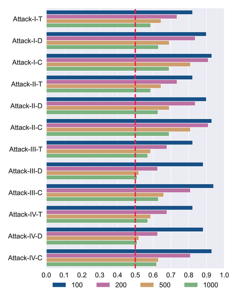
Our approach aligns with other membership inference attacks against diffusion models [7, 61, 12, 6]. We aim to employ Differential Privacy Stochastic Gradient Descent (DP-SGD) [1] to evaluate the robustness of our attack. The primary purpose of this defense method is to prevent the inference of training samples from the model by diminishing the model’s memorization of individual samples, achieved by introducing noise into the gradient updates during model training. Implementing DP-SGD in other membership inference attacks targeting diffusion models [61, 12, 6] has consistently hindered normal model convergence, resulting in the generation of low-quality images.

Figure 9: Results of attacks with DP-SGD: Despite the implementation of defenses, the attacks still retain partial effectiveness.

We employed a classifier as the attack inference model to test against the MS COCO dataset. The results indicate that the success rate of the attack significantly decreases after implementing DP-SGD [1] as a defensive measure. Figure 9 illustrates that the accuracy of Attack-III and Attack-IV is significantly impacted, dropping to around $60\%$, whereas Attack-I and Attack-II still maintain a success rate close to $70\%$.

We hypothesize that our attack relies on the model’s memorization of training data, which enables the use of similarity scores as an indicator for assessment. However, the application of DP-SGD reduces the model’s memorization capacity for training data, leading to decreased similarity scores in member set samples and, resulting in a lower attack success rate. The higher attack accuracy of Attack-I and Attack-II can be attributed to the overlap between the member sets of the shadow models and the training set of the target models.

7 Related Work

We review further related works on membership inference attacks (MIAs) and extraction attacks against diffusion models.

7.1 White-Box MIA

In the white-box setting, the attacker has access to the parameters of the victim model. Note that in MIA for classification tasks, it is observed that having black-box means can sufficient enough information(i.e., predict vector [8, 21, 22, 32, 50, 51], top-k confidence score [47, 51]); but in MIA for generative models, because the model is more complicated and directly applying existing MIAs is not successful, white-box attacks are investigated.

Both Hu et al. [20] and Matsumoto et al. [34] adopt approaches similar to that of Yeom et al. [62], determining membership by comparing the loss at various timesteps to a specific threshold. Carlini et al. [6] argue that mere threshold-based determinations are insufficient and proposed training multiple shadow models and utilizing the distribution of loss across each timestep established by these shadow models to execute an online LiRA attack [5]. Pang et al. [37] leveraged the norm of gradient information computed from timesteps uniformly sampled across total diffusion steps as attack data to train their attack model.

7.2 Gray-box MIA

Gray-box access does not acquire any internal information from the model. However, given that diffusion models generate images through a progressive denoising process, attacks in this setting assume the availability of intermediate outputs during this process. In particular, Duan et al. [12] and Kong et al. [25] leveraged the deterministic properties of generative process in DDIM [54] for their attack designs. Duan et al. [12] employed the approximated posterior estimation error as attack features, while Kong et al. [25] used the magnitude difference $\lVert x_{t-t^{\prime}}-x^{\prime}_{t-t^{\prime}}\rVert_{p}$ from the denoising process as their attack criterion, where $x_{t-t^{\prime}}$ represents the ground truth and $x^{\prime}_{t-t^{\prime}}$ denotes the predicted value. Fu et al. [14] use the intermediate output to calculate the probabilistic fluctuations between target points and neighboring points.

7.3 Extracting Attack

In recent few years, not only do the owners of models potentially infringe upon privacy through the misuse of data in training, but users of the models may also violate privacy by extracting sensitive training data from the models. This is particularly concerning for image generation models trained on high-value data, such as medical imaging models [52]. The training data for these models constitute private information. However, there currently exist extracting attacks targeting generative models [6], capable of extracting training samples from the models. Undoubtedly, this poses a significant infringement on the intellectual property rights of the model owners.

Carlini et al. [6] posited that models are more prone to memorizing duplicated samples, a hypothesis central to their strategy for extracting data attack. Rather than a bit-by-bit comparison, they opted for comparing CLIP embeddings due to the dataset’s vast size. This approach facilitated the identification of potential duplicates based on the $\ell_{2}$ distance between samples. The crux of their attack involved using the captions of these identified duplicates. Specifically, for each duplicated image, its corresponding caption was input $500$ times, generating $500$ candidate images. These images were then analyzed within a constructed graph, where connections were drawn between pairs of candidate images separated by less than a threshold distance $d$. The key indicator of a successful attack was the identification of the largest clique in the graph, comprising at least $10$ nodes, which was considered evidence of a memorized image.

8 Conclusion

In this work, we introduce a black-box membership inference attack framework specifically designed for contemporary conditional diffusion models. Given the rapid development of diffusion models and the abundance of open-source pre-trained models available online, we focus on the potential privacy issues arising from utilizing these pre-trained models fine-tuned for downstream tasks. Recognizing the absence of effective attacks against the current generation of conditional image generators, we leverage the objective function of diffusion models to propose a black-box similarity scores-based membership inference attack. Our experiments not only demonstrate the flexibility and effectiveness of this attack but also highlight significant privacy vulnerabilities in image generators, underscoring the need for increased attention to these issues.

However, our attacks still face certain limitations. As discussed in Section 5.8, both Attack-II and Attack-IV critically rely on a captioning model that has been fine-tuned using an auxiliary dataset. We hope future work can effectively address this challenge.

Appendix A More Details for Diffusion Models

Diffusion models have two phases: the forward diffusion process and the reverse denoising process. In the forward process, an image $x$ is sampled from the true data distribution. The image $x$ undergoes a series of noise addition steps for $T$ iterations, resulting in a sequence $x_{1},x_{2},\ldots,x_{T-1},x_{T}$, until $x_{T}$ becomes an image equation to an isotropic Gaussian noise distribution. The magnitude of noise introduced at each step is controlled by a parameter $\alpha_{t}$, where $\alpha_{t}\in[0,1]$, which gradually decreases over time. At step $t$, the noise image $x_{t}$ can be represent as:

$$x_{t}=\sqrt{\alpha_{t}}x_{t-1}+\sqrt{1-\alpha_{t}}\epsilon;\quad\epsilon\sim\mathcal{N}(0,1)$$

Given that the original work [18] considers the forward process as a Markov chain and employs the reparameterization trick, it is possible to directly derive the noisy image $x_{t}$ at step $t$ from the original image $x_{0}$.

Given the definition $\bar{\alpha}_{t}=\prod_{i=1}^{t}\alpha_{i}$, the training objective for diffusion models is to obtain a denoising network capable of sampling $x_{t-1}$ from $x_{t}$ according to the distribution $\mathcal{N}(x_{t-1};\mu_{\theta}(x_{t},t),\sigma_{t}^{2}\text{I})$. When conditioned on $x_{0}$ and $x_{t}$ from $q(x_{t-1}|x_{t},x_{0})$, the ground-truth distribution of $x_{t-1}$ is given by $\mathcal{N}(x_{t-1};\tilde{\mu}_{t}(x_{t},x_{0}),\sigma_{t}^{2}\text{I})$. Given that the variance is fixed as a hyperparameter, the focus is on calculating the difference between $\mu_{\theta}(x_{t},t)$ and $\tilde{\mu}_{t}(x_{t},x_{0})$. Applying Bayes’ rule to the ground-truth distribution

$$\tilde{\mu}_{t}(x_{t},x_{0})=\frac{\sqrt{\alpha_{t}}(1-\bar{\alpha}_{t-1})}{1-\bar{\alpha}_{t}}x_{t}+\frac{\sqrt{\bar{\alpha}_{t-1}}(1-\alpha_{t})}{1-\bar{\alpha}_{t}}x_{0}$$ (11)

The objective of the training process is to closely approximate $\mu_{\theta}(x_{t},t)$ with $\tilde{\mu}_{t}(x_{t},x_{0})$. Then, parameterize

$$\mu_{\theta}(x_{t},t)=\frac{\sqrt{\alpha_{t}}(1-\bar{\alpha}_{t-1})}{1-\bar{\alpha}_{t}}x_{t}+\frac{\sqrt{\bar{\alpha}_{t-1}}(1-\alpha_{t})}{1-\bar{\alpha}_{t}}\hat{x}_{\theta}(x_{t},t)$$ (12)

As a result, by deriving $x_{t}$ from $x_{0}$ using Equation 1 and omitting the weight term as suggested by Ho et al. [18], the loss function can be articulated as presented in Equation 2.

Appendix B More Details for Classifier-free Guidance

As the field continues to evolve, diffusion models have the capability to generate content based on user-provided conditional prompts, a key mechanism of which is classifier-free guidance [19]. Many diffusion models, including Imagen [46], DALL·E 2 [40], and Stable Diffusion [44], which utilize the classifier-free guidance mechanism, are trained on dual objectives; however, they can be represented with a single model during training by probabilistically setting the conditional prompt to null. A conditional generation without an explicit classifier is achieved using the denoising network $\bar{\mathcal{U}}_{\theta}(x_{t},t,y)$, where

$$\bar{\mathcal{U}}_{\theta}(x_{t},t,y)=(w+1)\cdot\mathcal{U}_{\theta}(x_{t},t,y)-w\cdot\mathcal{U}_{\theta}(x_{t},t).$$

The variable $w$ represents the guidance scale factor, where a higher value of $w$ results in improved alignment between image and text at the potential expense of image fidelity.

Appendix C More Details for Traditional Black-box Attacks

In this section, we will discuss some of the most influential prior works on black-box attacks targeting image-generative models.

Monte Carlo Attack.

Hilprecht et al. [17] argue that generative models, due to their inherent ability to capture data specifics, can exhibit overfitting and memorization. Given a query sample $x$, attackers can utilize the generative model to sample $k$ images. Define an $\epsilon$-neighborhood set $U_{\epsilon}(x)$ as $U_{\epsilon}(x)=\{x^{\prime}\mid d(x,x^{\prime})\leq\epsilon\}$. Intuitively, if a larger number of $g_{i}$ are close to $x$, the probability $\mathsf{Pr}\left[x^{\prime}\in U_{\epsilon}(x)\right]$ will also be greater. Through the Monte Carlo Integration [36], the Monte Carlo attack can be expressed as:

$$\hat{f}_{MC-\epsilon}(x)=\frac{1}{k}\sum_{i=1}^{k}\mathbbm{1}_{x^{\prime}_{i}\in U_{\epsilon}(x)}$$ (13)

Furthermore, they try to employ the Kernel Density Estimator (KDE) [38] as a substitute for $\hat{f}_{MC-\epsilon}(x)$. The estimation of the likelihood of $x$ using KDE can be expressed as:

$$\hat{f}_{KDE}(x)=\frac{1}{nh^{d}}\sum^{k}_{i=1}K\left(\frac{x-x^{\prime}_{i}}{h^{d}}\right)$$

where $h_{d}$ is the bandwidth and $K$ is the Gaussian kernel function. If $x\in\mathbf{D}_{m}$, the likelihood $\hat{f}_{KDE}(x)$ should be substantially higher than the likelihood when $x\in\mathbf{D}_{nm}$. However, upon experimentation, it was observed that using $\hat{f}_{KDE}(x)$ as the criterion for the attack did not yield attack accuracy better than random guessing.

GAN-Leaks Attack.

In a further examination of the memorization and overfitting phenomena associated with generative models, Chen et al. [7] posited that the closer the generated data distribution $p_{\theta}(\hat{x})$ is to the training data distribution $q(x)$, the more likely it is for $\mathcal{M}$ to generate a query datapoint $x$. They further articulated this observation as:

$$\mathsf{Pr}\left[y_{q}=1|x,\theta\right]\propto\mathsf{Pr}_{\mathcal{M}}[x|\theta_{v}]$$

However, due to the inability to represent the distribution of generated data with an explicit density function, computing the precise probability becomes intractable. Consequently, Chen et al. [7] also employed the KDE method [38] and sampled $k$ times to estimate the likelihood of $x$. This can be expressed as:

$$\mathsf{Pr}_{\mathcal{M}}(x|\theta)=\frac{1}{k}\sum_{i=1}^{k}K(x,\mathcal{M}(z_{i}));\quad z_{i}\sim P_{z}$$ (14)

Here, $K$ denotes the kernel function, and $z_{i}$ represents the input to $\mathcal{M}$, which sample from latent code distribution $P_{z}$. Besides, Chen et al. [7] propose the approximation of Equation 14:

$$\mathsf{Pr}_{\mathcal{M}}(x|\theta_{v})\approx\frac{1}{k}\sum_{i=1}^{k}\text{exp}(-d(x,\mathcal{M}(z_{i})));\quad z_{i}\sim P_{z}$$ (15)

For the $k$ samples generated by $\mathcal{M}$, the distance metric $d(\cdot,\cdot)$ is employed to compute the distance between each sample $g_{i}$ and the query point $x$, and then summed up. Equation 13 and Equation 15 convey very similar meanings, for models with such undetermined sampling, the only feasible method to increase the attack success rate is through a substantial number of sampled data $g_{i}$. For a full-black attack, around $100k$ samples are required for a query point $x$ to achieve an attack AUC close to $0.60$. This undoubtedly results in significant overhead. Then, Chen et al. [7] introduced the concept of a partial-black attack. Specifically, the attacker first employs

$$z^{\ast}=\underset{z}{\mathrm{arg\,min}}L(x,\mathcal{M}(z))$$

to identify the optimal latent code $z^{\ast}$. Subsequently, $g_{i}$ is generated using $\mathcal{M}(z^{\ast})$ to compare with $x$. This partial-black attack approach indeed consistently improves the success rate of attacks and reduces the number of sampled data points. However, the trade-off is the necessity to identify the optimal $z^{\ast}$. For GAN models, the input latent code $z$ is a 100-dimensional random noise. However, for contemporary conditional diffusion models, the dimensionality of the input embedding has increased exponentially. Moreover, for the latest generation of diffusion models, the input is no longer an undetermined latent code but can be explicit prompt information. Therefore, the partial-black attack tailored for GAN models is no longer applicable to these new-generation generative models.

Appendix D More Experimental Results from Varying Fine-tuning Steps

In this part, we want to examine the impact of increasing fine-tuned steps on the outcomes of different types of attacks. The distribution-based attack results can be found in Figure 10, and the threshold-based attack is illustrated in Figure 11.

Figure 10: Correlation between increased fine-tuning steps and enhanced accuracy of distribution-based attack.

Figure 11: Increase in success rate of threshold-based attack with more fine-tuning steps

Appendix E More Experimental Results for Different Number of Inference Steps

To evaluate how inference steps affect attack accuracy, we conducted experiments on the WIT and MS COCO datasets, with results detailed in Table VI and Table VII.

TABLE VI: Influence of inference step count on MS COCO.

S	Threshold-based			Distribution-based			Classifier-based			FID
	ASR	AUC	T@F=1%	ASR	AUC	T@F=1%	ASR	AUC	T@F=1%
30	$0.76$	$0.84$	$0.13$	$0.70$	$0.77$	$0.13$	$0.84$	$0.90$	$0.42$	$8.49$
50	$0.74$	$0.84$	$0.13$	$0.69$	$0.77$	$0.11$	$0.84$	$0.91$	$0.20$	$7.24$
100	$0.76$	$0.84$	$0.15$	$0.70$	$0.76$	$0.11$	$0.85$	$0.90$	$0.23$	$6.46$
200	$0.77$	$0.84$	$0.16$	$0.71$	$0.75$	$0.11$	$0.83$	$0.88$	$0.21$	$6.46$

TABLE VII: Impact of inference step count on WIT.

S	Threshold-based			Distribution-based			Classifier-based			FID
	ASR	AUC	T@F=1%	ASR	AUC	T@F=1%	ASR	AUC	T@F=1%
30	$0.71$	$0.81$	$0.23$	$0.61$	$0.70$	$0.26$	$0.78$	$0.82$	$0.29$	$6.73$
50	$0.71$	$0.80$	$0.20$	$0.62$	$0.72$	$0.25$	$0.75$	$0.82$	$0.30$	$5.83$
100	$0.71$	$0.79$	$0.17$	$0.65$	$0.74$	$0.09$	$0.76$	$0.83$	$0.32$	$5.58$
200	$0.70$	$0.79$	$0.20$	$0.62$	$0.72$	$0.14$	$0.77$	$0.83$	$0.33$	$5.56$

Appendix F More Details for Comparing Five Different Image Encoders

To comprehensively analyze the influence of various image feature extractors on attack success rates, we evaluated the performance of five distinct image feature extractors across three types of attacks, within four attack scenarios obtained by the attacker, on three datasets.

TABLE VIII: Comparative analysis of five different image encoders using threshold-based attack across three datasets.

		DETR			BEiT			EfficientFormer			ViT			DeiT
		ASR	AUC	T@F=1%	ASR	AUC	T@F=1%	ASR	AUC	T@F=1%	ASR	AUC	T@F=1%	ASR	AUC	T@F=1%
CelebA	Attack-I	$0.57$	$0.64$	$0.02$	$0.79$	$0.86$	$0.41$	$0.70$	$0.76$	$0.26$	$0.73$	$0.78$	$0.01$	$0.75$	$0.82$	$0.43$
	Attack-II	$0.60$	$0.64$	$0.02$	$0.77$	$0.86$	$0.41$	$0.70$	$0.76$	$0.29$	$0.73$	$0.78$	$0.18$	$0.76$	$0.82$	$0.45$
	Attack-III	$0.57$	$0.65$	$0.01$	$0.79$	$0.86$	$0.40$	$0.71$	$0.76$	$0.23$	$0.67$	$0.79$	$0.12$	$0.75$	$0.82$	$0.20$
	Attack-IV	$0.59$	$0.66$	$0.05$	$0.78$	$0.86$	$0.39$	$0.68$	$0.76$	$0.24$	$0.69$	$0.76$	$0.13$	$0.77$	$0.84$	$0.32$
WIT	Attack-I	$0.59$	$0.66$	$0.07$	$0.56$	$0.62$	$0.06$	$0.66$	$0.76$	$0.12$	$0.72$	$0.79$	$0.02$	$0.68$	$0.77$	$0.17$
	Attack-II	$0.57$	$0.66$	$0.14$	$0.57$	$0.62$	$0.05$	$0.61$	$0.70$	$0.03$	$0.57$	$0.61$	$0.01$	$0.62$	$0.67$	$0.02$
	Attack-III	$0.60$	$0.66$	$0.02$	$0.60$	$0.61$	$0.03$	$0.66$	$0.71$	$0.09$	$0.63$	$0.71$	$0.03$	$0.64$	$0.69$	$0.13$
	Attack-IV	$0.57$	$0.62$	$0.01$	$0.66$	$0.73$	$0.03$	$0.69$	$0.80$	$0.13$	$0.70$	$0.82$	$0.02$	$0.73$	$0.80$	$0.20$
MS COCO	Attack-I	$0.71$	$0.73$	$0.01$	$0.71$	$0.80$	$0.14$	$0.74$	$0.82$	$0.11$	$0.68$	$0.77$	$0.17$	$0.79$	$0.84$	$0.05$
	Attack-II	$0.63$	$0.72$	$0.01$	$0.75$	$0.80$	$0.15$	$0.75$	$0.82$	$0.11$	$0.70$	$0.78$	$0.18$	$0.79$	$0.85$	$0.06$
	Attack-III	$0.63$	$0.72$	$0.01$	$0.69$	$0.81$	$0.23$	$0.76$	$0.82$	$0.15$	$0.68$	$0.79$	$0.01$	$0.76$	$0.84$	$0.13$
	Attack-IV	$0.61$	$0.72$	$0.09$	$0.71$	$0.81$	$0.24$	$0.78$	$0.82$	$0.17$	$0.68$	$0.79$	$0.24$	$0.70$	$0.74$	$0.01$

TABLE IX: Comparative analysis of five different image encoders using distribution-based attack across three datasets.

		DETR			BEiT			EfficientFormer			ViT			DeiT
		ASR	AUC	T@F=1%	ASR	AUC	T@F=1%	ASR	AUC	T@F=1%	ASR	AUC	T@F=1%	ASR	AUC	T@F=1%
CelebA	Attack-I	$0.62$	$0.66$	$0.03$	$0.76$	$0.90$	$0.65$	$0.70$	$0.83$	$0.41$	$0.74$	$0.84$	$0.40$	$0.73$	$0.90$	$0.61$
	Attack-II	$0.61$	$0.66$	$0.03$	$0.79$	$0.90$	$0.66$	$0.71$	$0.82$	$0.32$	$0.73$	$0.85$	$0.39$	$0.74$	$0.90$	$0.64$
	Attack-III	$0.56$	$0.58$	$0.01$	$0.74$	$0.85$	$0.51$	$0.61$	$0.71$	$0.20$	$0.64$	$0.74$	$0.13$	$0.76$	$0.88$	$0.50$
	Attack-IV	$0.59$	$0.61$	$0.01$	$0.72$	$0.86$	$0.61$	$0.61$	$0.70$	$0.21$	$0.67$	$0.73$	$0.16$	$0.77$	$0.88$	$0.52$
WIT	Attack-I	$0.66$	$0.72$	$0.12$	$0.70$	$0.83$	$0.27$	$0.70$	$0.82$	$0.22$	$0.70$	$0.85$	$0.30$	$0.69$	$0.84$	$0.41$
	Attack-II	$0.58$	$0.68$	$0.07$	$0.70$	$0.81$	$0.14$	$0.66$	$0.78$	$0.19$	$0.71$	$0.84$	$0.23$	$0.68$	$0.84$	$0.34$
	Attack-III	$0.57$	$0.57$	$0.01$	$0.62$	$0.69$	$0.15$	$0.62$	$0.68$	$0.20$	$0.60$	$0.67$	$0.10$	$0.61$	$0.70$	$0.26$
	Attack-IV	$0.51$	$0.55$	$0.01$	$0.61$	$0.71$	$0.14$	$0.60$	$0.66$	$0.23$	$0.56$	$0.64$	$0.11$	$0.64$	$0.69$	$0.09$
MS COCO	Attack-I	$0.62$	$0.71$	$0.19$	$0.65$	$0.80$	$0.33$	$0.67$	$0.79$	$0.14$	$0.59$	$0.73$	$0.43$	$0.73$	$0.81$	$0.36$
	Attack-II	$0.60$	$0.71$	$0.18$	$0.64$	$0.80$	$0.32$	$0.68$	$0.80$	$0.15$	$0.61$	$0.74$	$0.41$	$0.72$	$0.81$	$0.36$
	Attack-III	$0.56$	$0.57$	$0.03$	$0.62$	$0.70$	$0.09$	$0.61$	$0.63$	$0.10$	$0.61$	$0.67$	$0.06$	$0.70$	$0.77$	$0.13$
	Attack-IV	$0.55$	$0.57$	$0.02$	$0.63$	$0.70$	$0.06$	$0.59$	$0.63$	$0.12$	$0.62$	$0.67$	$0.07$	$0.62$	$0.67$	$0.07$

TABLE X: Comparative analysis of five different image encoders using classifier-based attack across three datasets.

		DETR			BEiT			EfficientFormer			ViT			DeiT
		ASR	AUC	T@F=1%	ASR	AUC	T@F=1%	ASR	AUC	T@F=1%	ASR	AUC	T@F=1%	ASR	AUC	T@F=1%
CelebA	Attack-I	$0.66$	$0.70$	$0.10$	$0.87$	$0.95$	$0.64$	$0.80$	$0.87$	$0.37$	$0.81$	$0.88$	$0.26$	$0.87$	$0.93$	$0.49$
	Attack-II	$0.67$	$0.69$	$0.09$	$0.88$	$0.94$	$0.57$	$0.82$	$0.88$	$0.38$	$0.80$	$0.88$	$0.29$	$0.88$	$0.94$	$0.61$
	Attack-III	$0.67$	$0.71$	$0.07$	$0.84$	$0.91$	$0.57$	$0.81$	$0.87$	$0.42$	$0.79$	$0.83$	$0.40$	$0.87$	$0.94$	$0.52$
	Attack-IV	$0.67$	$0.71$	$0.10$	$0.84$	$0.91$	$0.58$	$0.78$	$0.84$	$0.44$	$0.78$	$0.83$	$0.38$	$0.88$	$0.933$	$0.60$
WIT	Attack-I	$0.74$	$0.79$	$0.11$	$0.70$	$0.80$	$0.30$	$0.76$	$0.81$	$0.13$	$0.77$	$0.83$	$0.06$	$0.79$	$0.84$	$0.22$
	Attack-II	$0.73$	$0.77$	$0.10$	$0.69$	$0.77$	$0.27$	$0.71$	$0.78$	$0.11$	$0.74$	$0.80$	$0.16$	$0.78$	$0.85$	$0.15$
	Attack-III	$0.65$	$0.72$	$0.07$	$0.71$	$0.78$	$0.17$	$0.78$	$0.82$	$0.22$	$0.78$	$0.82$	$0.21$	$0.77$	$0.83$	$0.29$
	Attack-IV	$0.64$	$0.69$	$0.08$	$0.72$	$0.77$	$0.11$	$0.76$	$0.81$	$0.16$	$0.77$	$0.82$	$0.05$	$0.75$	$0.83$	$0.25$
MS COCO	Attack-I	$0.72$	$0.75$	$0.17$	$0.77$	$0.84$	$0.24$	$0.78$	$0.87$	$0.20$	$0.73$	$0.82$	$0.20$	$0.85$	$0.93$	$0.61$
	Attack-II	$0.75$	$0.80$	$0.06$	$0.77$	$0.85$	$0.16$	$0.81$	$0.87$	$0.35$	$0.75$	$0.83$	$0.20$	$0.85$	$0.92$	$0.56$
	Attack-III	$0.70$	$0.78$	$0.16$	$0.78$	$0.84$	$0.44$	$0.78$	$0.82$	$0.28$	$0.71$	$0.80$	$0.20$	$0.83$	$0.89$	$0.30$
	Attack-IV	$0.70$	$0.76$	$0.20$	$0.80$	$0.83$	$0.40$	$0.76$	$0.83$	$0.27$	$0.75$	$0.82$	$0.31$	$0.69$	$0.74$	$0.16$

References

- [1] Martin Abadi, Andy Chu, Ian Goodfellow, H. Brendan McMahan, Ilya Mironov, Kunal Talwar, and Li Zhang. Deep learning with differential privacy. In Proceedings of the 2016 ACM SIGSAC Conference on Computer and Communications Security. ACM, oct 2016.
- [2] Hangbo Bao, Li Dong, Songhao Piao, and Furu Wei. Beit: Bert pre-training of image transformers, 2022.
- [3] James Betker, Gabriel Goh, Li Jing, † TimBrooks, Jianfeng Wang, Linjie Li, † LongOuyang, † JuntangZhuang, † JoyceLee, † YufeiGuo, † WesamManassra, † PrafullaDhariwal, † CaseyChu, † YunxinJiao, and Aditya Ramesh. Improving image generation with better captions.
- [4] Nicolas Carion, Francisco Massa, Gabriel Synnaeve, Nicolas Usunier, Alexander Kirillov, and Sergey Zagoruyko. End-to-end object detection with transformers, 2020.
- [5] Nicholas Carlini, Steve Chien, Milad Nasr, Shuang Song, Andreas Terzis, and Florian Tramer. Membership inference attacks from first principles, 2022.
- [6] Nicholas Carlini, Jamie Hayes, Milad Nasr, Matthew Jagielski, Vikash Sehwag, Florian Tramer, Borja Balle, Daphne Ippolito, and Eric Wallace. Extracting training data from diffusion models. arXiv preprint arXiv:2301.13188, 2023.
- [7] Dingfan Chen, Ning Yu, Yang Zhang, and Mario Fritz. Gan-leaks: A taxonomy of membership inference attacks against generative models. In Proceedings of the 2020 ACM SIGSAC conference on computer and communications security, pages 343–362, 2020.
- [8] Min Chen, Zhikun Zhang, Tianhao Wang, Michael Backes, Mathias Humbert, and Yang Zhang. When machine unlearning jeopardizes privacy. In Proceedings of the 2021 ACM SIGSAC Conference on Computer and Communications Security, CCS ’21. ACM, November 2021.
- [9] Christopher A. Choquette-Choo, Florian Tramer, Nicholas Carlini, and Nicolas Papernot. Label-only membership inference attacks, 2021.
- [10] Tim Dockhorn, Tianshi Cao, Arash Vahdat, and Karsten Kreis. Differentially private diffusion models, 2023.
- [11] Alexey Dosovitskiy, Lucas Beyer, Alexander Kolesnikov, Dirk Weissenborn, Xiaohua Zhai, Thomas Unterthiner, Mostafa Dehghani, Matthias Minderer, Georg Heigold, Sylvain Gelly, Jakob Uszkoreit, and Neil Houlsby. An image is worth 16x16 words: Transformers for image recognition at scale, 2021.
- [12] Jinhao Duan, Fei Kong, Shiqi Wang, Xiaoshuang Shi, and Kaidi Xu. Are diffusion models vulnerable to membership inference attacks?, 2023.
- [13] Virginia Fernandez, Pedro Sanchez, Walter Hugo Lopez Pinaya, Grzegorz Jacenków, Sotirios A. Tsaftaris, and Jorge Cardoso. Privacy distillation: Reducing re-identification risk of multimodal diffusion models, 2023.
- [14] Wenjie Fu, Huandong Wang, Chen Gao, Guanghua Liu, Yong Li, and Tao Jiang. A probabilistic fluctuation based membership inference attack for diffusion models, 2023.
- [15] Ian J. Goodfellow, Jean Pouget-Abadie, Mehdi Mirza, Bing Xu, David Warde-Farley, Sherjil Ozair, Aaron Courville, and Yoshua Bengio. Generative adversarial networks, 2014.
- [16] Shuyang Gu, Dong Chen, Jianmin Bao, Fang Wen, Bo Zhang, Dongdong Chen, Lu Yuan, and Baining Guo. Vector quantized diffusion model for text-to-image synthesis, 2022.
- [17] Benjamin Hilprecht, Martin Härterich, and Daniel Bernau. Monte carlo and reconstruction membership inference attacks against generative models. Proceedings on Privacy Enhancing Technologies, 2019:232 – 249, 2019.
- [18] Jonathan Ho, Ajay Jain, and Pieter Abbeel. Denoising diffusion probabilistic models, 2020.
- [19] Jonathan Ho and Tim Salimans. Classifier-free diffusion guidance, 2022.
- [20] Hailong Hu and Jun Pang. Membership inference of diffusion models. arXiv preprint arXiv:2301.09956, 2023.
- [21] Bo Hui, Yuchen Yang, Haolin Yuan, Philippe Burlina, Neil Zhenqiang Gong, and Yinzhi Cao. Practical blind membership inference attack via differential comparisons. In Proceedings 2021 Network and Distributed System Security Symposium. Internet Society, 2021.
- [22] Bargav Jayaraman, Lingxiao Wang, Katherine Knipmeyer, Quanquan Gu, and David Evans. Revisiting membership inference under realistic assumptions, 2021.
- [23] Yuming Jiang, Ziqi Huang, Xingang Pan, Chen Change Loy, and Ziwei Liu. Talk-to-edit: Fine-grained facial editing via dialog. In Proceedings of International Conference on Computer Vision (ICCV), 2021.
- [24] Diederik P Kingma and Max Welling. Auto-encoding variational bayes, 2022.
- [25] Fei Kong, Jinhao Duan, RuiPeng Ma, Hengtao Shen, Xiaofeng Zhu, Xiaoshuang Shi, and Kaidi Xu. An efficient membership inference attack for the diffusion model by proximal initialization, 2023.
- [26] Jiacheng Li, Ninghui Li, and Bruno Ribeiro. Membership inference attacks and defenses in classification models. In Proceedings of the Eleventh ACM Conference on Data and Application Security and Privacy. ACM, apr 2021.
- [27] Junnan Li, Dongxu Li, Silvio Savarese, and Steven Hoi. Blip-2: Bootstrapping language-image pre-training with frozen image encoders and large language models, 2023.
- [28] Kecen Li, Chen Gong, Zhixiang Li, Yuzhong Zhao, Xinwen Hou, and Tianhao Wang. Meticulously selecting 1
- [29] Yanyu Li, Geng Yuan, Yang Wen, Ju Hu, Georgios Evangelidis, Sergey Tulyakov, Yanzhi Wang, and Jian Ren. Efficientformer: Vision transformers at mobilenet speed, 2022.
- [30] Tsung-Yi Lin, Michael Maire, Serge Belongie, Lubomir Bourdev, Ross Girshick, James Hays, Pietro Perona, Deva Ramanan, C. Lawrence Zitnick, and Piotr Dollár. Microsoft coco: Common objects in context, 2015.
- [31] Yiyong Liu, Zhengyu Zhao, Michael Backes, and Yang Zhang. Membership inference attacks by exploiting loss trajectory, 2022.
- [32] Yunhui Long, Vincent Bindschaedler, Lei Wang, Diyue Bu, Xiaofeng Wang, Haixu Tang, Carl A. Gunter, and Kai Chen. Understanding membership inferences on well-generalized learning models, 2018.
- [33] Yunhui Long, Lei Wang, Diyue Bu, Vincent Bindschaedler, Xiaofeng Wang, Haixu Tang, Carl A. Gunter, and Kai Chen. A pragmatic approach to membership inferences on machine learning models. 2020 IEEE European Symposium on Security and Privacy (EuroS&P), pages 521–534, 2020.
- [34] Tomoya Matsumoto, Takayuki Miura, and Naoto Yanai. Membership inference attacks against diffusion models, 2023.
- [35] Alex Nichol, Prafulla Dhariwal, Aditya Ramesh, Pranav Shyam, Pamela Mishkin, Bob McGrew, Ilya Sutskever, and Mark Chen. Glide: Towards photorealistic image generation and editing with text-guided diffusion models, 2022.
- [36] Art B. Owen. Monte Carlo theory, methods and examples. https://artowen.su.domains/mc/, 2013.
- [37] Yan Pang, Tianhao Wang, Xuhui Kang, Mengdi Huai, and Yang Zhang. White-box membership inference attacks against diffusion models, 2023.
- [38] Emanuel Parzen. On estimation of a probability density function and mode. Annals of Mathematical Statistics, 33:1065–1076, 1962.
- [39] Sen Peng, Yufei Chen, Cong Wang, and Xiaohua Jia. Protecting the intellectual property of diffusion models by the watermark diffusion process, 2023.
- [40] Aditya Ramesh, Prafulla Dhariwal, Alex Nichol, Casey Chu, and Mark Chen. Hierarchical text-conditional image generation with clip latents, 2022.
- [41] Aditya Ramesh, Mikhail Pavlov, Gabriel Goh, Scott Gray, Chelsea Voss, Alec Radford, Mark Chen, and Ilya Sutskever. Zero-shot text-to-image generation. In International Conference on Machine Learning, pages 8821–8831. PMLR, 2021.
- [42] Anton Razzhigaev, Arseniy Shakhmatov, Anastasia Maltseva, Vladimir Arkhipkin, Igor Pavlov, Ilya Ryabov, Angelina Kuts, Alexander Panchenko, Andrey Kuznetsov, and Denis Dimitrov. Kandinsky: an improved text-to-image synthesis with image prior and latent diffusion. arXiv preprint arXiv:2310.03502, 2023.
- [43] Shahbaz Rezaei and Xin Liu. On the difficulty of membership inference attacks, 2021.
- [44] Robin Rombach, Andreas Blattmann, Dominik Lorenz, Patrick Esser, and Björn Ommer. High-resolution image synthesis with latent diffusion models. In Proceedings of the IEEE/CVF conference on computer vision and pattern recognition, pages 10684–10695, 2022.
- [45] Alexandre Sablayrolles, Matthijs Douze, Yann Ollivier, Cordelia Schmid, and Hervé Jégou. White-box vs black-box: Bayes optimal strategies for membership inference, 2019.
- [46] Chitwan Saharia, William Chan, Saurabh Saxena, Lala Li, Jay Whang, Emily Denton, Seyed Kamyar Seyed Ghasemipour, Burcu Karagol Ayan, S. Sara Mahdavi, Rapha Gontijo Lopes, Tim Salimans, Jonathan Ho, David J Fleet, and Mohammad Norouzi. Photorealistic text-to-image diffusion models with deep language understanding, 2022.
- [47] Ahmed Salem, Yang Zhang, Mathias Humbert, Pascal Berrang, Mario Fritz, and Michael Backes. Ml-leaks: Model and data independent membership inference attacks and defenses on machine learning models, 2018.
- [48] Christoph Schuhmann, Romain Beaumont, Richard Vencu, Cade Gordon, Ross Wightman, Mehdi Cherti, Theo Coombes, Aarush Katta, Clayton Mullis, Mitchell Wortsman, Patrick Schramowski, Srivatsa Kundurthy, Katherine Crowson, Ludwig Schmidt, Robert Kaczmarczyk, and Jenia Jitsev. Laion-5b: An open large-scale dataset for training next generation image-text models, 2022.
- [49] Shawn Shan, Jenna Cryan, Emily Wenger, Haitao Zheng, Rana Hanocka, and Ben Y. Zhao. Glaze: Protecting artists from style mimicry by text-to-image models, 2023.
- [50] Reza Shokri, Martin Strobel, and Yair Zick. On the privacy risks of model explanations, 2021.
- [51] Reza Shokri, Marco Stronati, Congzheng Song, and Vitaly Shmatikov. Membership inference attacks against machine learning models, 2017.
- [52] Nripendra Kumar Singh and Khalid Raza. Medical image generation using generative adversarial networks, 2020.
- [53] Jascha Sohl-Dickstein, Eric Weiss, Niru Maheswaranathan, and Surya Ganguli. Deep unsupervised learning using nonequilibrium thermodynamics. In International Conference on Machine Learning, pages 2256–2265. PMLR, 2015.
- [54] Jiaming Song, Chenlin Meng, and Stefano Ermon. Denoising diffusion implicit models, 2022.
- [55] Liwei Song and Prateek Mittal. Systematic evaluation of privacy risks of machine learning models, 2020.
- [56] Yang Song, Jascha Sohl-Dickstein, Diederik P. Kingma, Abhishek Kumar, Stefano Ermon, and Ben Poole. Score-based generative modeling through stochastic differential equations, 2021.
- [57] Krishna Srinivasan, Karthik Raman, Jiecao Chen, Michael Bendersky, and Marc Najork. Wit: Wikipedia-based image text dataset for multimodal multilingual machine learning. In Proceedings of the 44th International ACM SIGIR Conference on Research and Development in Information Retrieval, SIGIR ’21, page 2443–2449, New York, NY, USA, 2021. Association for Computing Machinery.
- [58] Fnu Suya, Anshuman Suri, Tingwei Zhang, Jingtao Hong, Yuan Tian, and David Evans. Sok: Pitfalls in evaluating black-box attacks. arXiv:2310.17534, 2023.
- [59] Hugo Touvron, Matthieu Cord, Matthijs Douze, Francisco Massa, Alexandre Sablayrolles, and Hervé Jégou. Training data-efficient image transformers & distillation through attention, 2021.
- [60] S. Truex, L. Liu, M. Gursoy, L. Yu, and W. Wei. Demystifying membership inference attacks in machine learning as a service. IEEE Transactions on Services Computing, 14(06):2073–2089, nov 2021.
- [61] Yixin Wu, Ning Yu, Zheng Li, Michael Backes, and Yang Zhang. Membership inference attacks against text-to-image generation models. arXiv preprint arXiv:2210.00968, 2022.
- [62] Samuel Yeom, Irene Giacomelli, Matt Fredrikson, and Somesh Jha. Privacy risk in machine learning: Analyzing the connection to overfitting, 2018.
- [63] Minxing Zhang, Ning Yu, Rui Wen, Michael Backes, and Yang Zhang. Generated distributions are all you need for membership inference attacks against generative models, 2023.