Spectral fluctuations of multi-parametric complex matrix ensembles: evidence of a single parameter dependence

Abstract

We numerically analyze the spectral statistics of the multiparametric Gaussian ensembles of complex matrices with zero mean and variances with different decay routes away from the diagonals. As the latter mimics different degree of effective sparsity among the matrix elements, such ensembles can serve as good models for a wide range of phase transitions e.g. localization to delocalization in non-Hermitian systems or Hermitian to non-Hermitian one. Our analysis reveals a rich behavior hidden beneath the spectral statistics e.g. a crossover of the spectral statistics from Poisson to Ginibre universality class with changing variances for finite matrix size, an abrupt transition for infinite matrix size and the role of complexity parameter, a single functional of all system parameters, as a criteria to determine critical point. We also confirm the theoretical predictions in [1], regarding the universality of the spectral statistics in non-equilibrium regime of non-Hermitian systems characterized by the complexity parameter.

.

I Introduction

Complex random matrices appear as the matrix representations of non-Hermitian operators of complex systems in diverse areas (e.g. see [2, 3, 4, 5, 6, 7, 8, 9, 10, 11, 12, 13, 14, 15, 16, 17, 18, 19, 20, 21, 22, 23, 24, 25, 26, 27, 28, 29, 30, 31, 32, 33, 34, 35, 36, 37, 38, 39, 40]). A knowledge of their statistical behavior is necessary to determine many of the physical properties. As the degree and type of randomness is often system specific and leads in general to a wide range of ensembles, it is desirable to seek a common mathematical formulation of their statistical behavior; this would not only help to probe a specific complex system but also in revealing the hidden connections among seemingly different complex systems.

The existence of a common mathematical formulation has been indicated in past for the Hermitian operators [41, 42, 43, 45, 46, 44, 47, 48] and is also verified by the detailed numerical analysis on many body as well as disordered systems. While a corresponding formulation for the non-Hermitian cases was first derived in [1] and further developed recently in [49] for the average spectral density, its detailed theoretical and numerical analysis on the complex plane e.g. the fluctuations of the radial and angular parts of the eigenvalues, and validity of complexity parameter based predictions was not pursued earlier (mainly due to lack of interest in non-Hermitian operators in past). We note that contrary to Hermitian case, the statistical behavior on the complex plane is far more richer, has many degrees of freedom and therefore technically far more complicated notwithstanding analogous basic mathematical skeletons in both the cases. Intense renewed interest in the statistics of non-Hermitian operators but lack of a theoretical formulation motivates us to pursue, in the present work, a detailed numerical analysis of the fluctuations.

As indicated by extensive studies, the statistical behavior of complex systems with ergodic wave dynamics can be well described by basis-invariant random matrix ensembles e.g. those with ensemble density dependent only on the trace of the matrix [48, 39]. In case of non-ergodic wave dynamics, however, the basis details affect the matrix representation of the complex system and lead to basis-non-invariant, multiparametric ensembles of random matrices. As intuitively expected, the details of the ensemble are often sensitive to underlying system conditions but the relevant exact information is usually obscured by underlying complexity leaving access only to some statistical parameters. Fortunately, based on the maximum entropy hypothesis, a knowledge of the latter is often sufficient to predict the nature of the distribution e.g. Gaussian if the average and variance of the matrix elements are known. This motivates us to consider a complex system, e.g a Hamiltonian with complicated many body interactions, represented by a complex matrix $H$ in an arbitrary orthonormal basis and with known constraints only on the mean and variances of the matrix elements $H_{kl}$ and their pair wise correlations. Based on the maximum entropy hypothesis (MEH), it can then be described by an ensemble of $N\times N$ complex matrices $H$ defined by a Gaussian ensemble density

$$\tilde{\rho}(H,y,x)=C\;{\rm exp}\left[-\sum_{s=1}^{2}\sum_{k,l}(y_{kl;s}H_{kl;s}^{2}+x_{kl;s}H_{kl;s}H_{lk;s})\right]$$ (1)

with $C$ as the normalization constant, $y$ and $x$ as the sets of variances and covariances of various matrix elements, and, the subscript $s$ on a variable refers to one of its components, i.e real ($s=1$) or imaginary ($s=2$).

For an ensemble to be an appropriate representation of the physical system of interest, the ensemble parameters must be chosen as the functions of system parameters. As the ensemble parameters $y_{kl;s},x_{kl;s}$ in eq.(1) can be arbitrarily chosen (including an infinite value for non-random entries), this enables $\rho(H,y,x)$ to represent a large class of non-Hermitian matrix ensembles e.g. varying degree of sparsity or bandedness. Further by a variation of $y_{kl;s},x_{kl;s}$, eq.(1) can also be used as a model to analyze a wide range of crossovers/ transitions e.g. from Hermitian to non-Hermitian system conditions, from one non-Hermitian universality class to another one e.g. Poisson to Ginibre universality class [1].

The standard route for the statistical analysis of a random matrix ensemble is based on the fluctuation measures of its eigenvalues and eigenfunctions and requires, in turn, a knowledge of their joint probability distribution function (JPDF). An integration of the latter over undesired variables then, in principle, leads to the correlation functions for the remaining variables e.g. the spectral correlations resulting from an integration over all eigenfunction components. The integration is technically easier if the ensemble density is basis invariant e.g. depends only on the trace of the matrix [48]. Except for the basis invariant cases, an integration of the ensemble density is in general technically complicated and a search for alternative routes is necessary. As discussed in [1], a differential equation for the spectral JPDF for non-Hermitian multiparametric Gaussian ensembles can be derived from the ensemble density but a derivation of local fluctuation measures from the equation is again not an easy task and requires theoretical approximations. To gain an insight about the latter, it is instructive to first pursue a numerical investigation of the ensembles. Our focus in the present work is on following objectives:

(i) to establish whether the measures satisfy local ergodicity assumption (needed to approximate spectral averages by the ensemble ones)

(ii) to analyze crossover of the fluctuation measures between Poisson and Ginibre universality class with varying ensemble parameters,

(iii) to analyze size-dependence of the fluctuation measures and seek critical spectral statistics,

(iv) to verify that different ensembles exhibit same spectral statistics if their complexity parameters are same and if they have same initial conditions.

The motivation for the first objective arises from the rich physics reported for non-Hermitian many body systems with non-ergodic dynamics. The ergodic dynamics is a necessary tool for system’s approach to thermalization and thereby permitting application of standard statistical tools e.g. equivalence assumption of spectral with ensemble averages. While the spectral density for non-ergodic systems is in general non-ergodic, this does not rule out local ergodicity of local fluctuation measures. and requires a numerical verification. The necessity for the second objective lies in the unavoidable presence of disorder as well as many body interactions in physical systems which can manifests in a variety of ways in the matrix representation of their non-Hermitian operators; it is natural to query whether presence of disorder with/ without interactions has any, and if so, what impact on the fluctuations of the excitations over representative ensemble and can these fluctuations mimic, at least locally, the fluctuations on a single spectral plane? .

A complex system often acts in an infinite dimensional Hilbert space and the random matrices in its representative ensemble are therefore of infinite size. The numerical analysis however involves only finite size matrices. For application of the numerical information to real systems, it is necessary to analyze how far the approximations and insights based on finite sizes be extended to infinite sizes e.g. due to some scaling relations and is the basis of our third objective.

The quest for the fourth objective originates from the significant claim made in the study [1], indicating the existence of a single parameter governed common evolution equation for the spectral correlations for a wide range of physical systems represented by the Gaussian non-Hermitian random matrix ensembles. The system dependence in the formulation enters through the complexity parameter $Y$, a function of ensemble parameters and thereby a functional of system parameters [1]. The common evolution equation predicts the analogy of the statistical fluctuations for different non Hermitian Gaussian ensembles if their rescaled $Y$ values as well as the initial conditions are same. This in turn claims an existence of universality in non-equilibrium regime of the ensemble representing a complex system (subjected to random perturbations); the significance of the claim requires therefore a detailed numerical verification.

The paper is organized as follows. To keep the present work self contained, Section II briefly reviews the relevant steps of detailed theoretical formulation derived in [1]. Section III presents the ensemble densities for the cases considered in our numerical analysis; To fulfil our objectives, here we numerically analyze complex matrix ensembles for three different type of off-diagonal variances; these ensembles are special cases of the ensemble density eq.(1). An analysis of the spectral fluctuation measures requires a specific rescaling of the spectrum which in turn depends on whether the spectrum is ergodic or not; this is discussed in section III. A along with a numerical study of the ergodicity for the three ensembles along with the Ginibre ensembles. Sections III.B and III.C present the numerical analysis of the fluctuations for each of the three ensembles for many system parameters; the objective of these sections is not only to verify that the crossover from initial to stationary state is indeed driven by a single function of all system conditions but also to provide insights about permissible approximations necessary for theoretical analysis of mathematically intractable fluctuation measures. Section III.D presents the details of a critical point analysis of the spectral statistics and reconfirm our theoretical predictions of [49]. We conclude in section IV with a brief reviews of our main results and open questions.

II Complexity parametric formulation of Spectral correlations

With ensemble (1) representing a non Hermitian operator $H$ in an $N$-dimensional Hilbert space, a typical matrix $H\equiv\left[H_{kl}\right]$ in the ensemble (1) is a $N\times N$ complex matrix. The eigenvalues $\lambda_{1},\ldots,\lambda_{N}$ of $H$ are distributed on the complex plane with $\langle U_{n}|$ and $|V_{n}\rangle$ as the left and right eigenvectors corresponding to $\lambda_{n}$: $\langle U_{n}|H=\lambda_{n}\langle U_{n}|$ and $H|V_{n}\rangle=\lambda_{n}|V_{n}\rangle$. The eigenvectors are defined up to multiplication by scalar constants and are bi-orthogonal i.e $\langle U_{m}|V_{n}\rangle=\delta_{mn}$. The eigenvalue spectrum is described by the equation $H=U\Lambda V$ with $\Lambda=\left[\lambda_{n}\delta_{mn}\right]$ as the eigenvalue matrix, $U\equiv\left[U_{kn}\right]$, $V\equiv\left[V_{kn}\right]$ as the left and right eigenvector matrices with $X_{kn}\equiv\langle k\mid X_{n}\rangle$ as the entries for $X=U,V$.

Following from eq.(1), the matrix elements of $H$ are randomly distributed. This in turn randomizes its eigenvalues and eigenfunctions thus rendering it imperative to consider their distributions. Confining present analysis to eigenvalues only, the joint probability density function (jpdf) $P(z_{1},z_{2},\ldots z_{N})$ for the eigenvalues $\lambda_{n}$ to occur at $z_{n}$ on the spectral plane can be defined as $P(z_{1},z_{2},\ldots z_{N})=\int\delta(Z-\Lambda)\;\rho(H)\;{\rm D}H$. A multiple integration of the latter gives the probability densities $R_{n}(z_{1},\ldots,z_{n};Y)$ for levels at each of the $n$ points $z_{1},\ldots,z_{n}$ on the spectral plane irrespective of the positions of the rest $N-n$ levels. Also referred as $n^{\rm th}$ order spectral density correlator or simply n-level correlation functions, $R_{n}$ can be defined as

$$R_{n}(z_{1},\ldots,z_{n})={N!\over{(N-n)!}}\int P(z_{1},\ldots,z_{N};Y)\,{\rm D}\Omega_{n+1}$$ (2)

with ${\rm D}\Omega_{n+1}\equiv\prod_{k=n+1}^{N}\;{\rm d}z_{k}\,{\rm d}z^{*}_{k}$. The case $n=1$ corresponds to the ensemble averaged spectral density $R_{1}$. Alternatively, assuming the spectral density $\rho(z)$ consisting of a secular part superimposed by a fluctuating part i.e $\rho(z)=\langle\rho(z)\rangle+\delta\rho(z)$, $R_{n}$ can also be defined as the correlation between $n$-point fluctuations of $\rho(z)$: $R_{n}(z_{1},\ldots,z_{n})=\langle\delta\rho(z_{1})\ldots\delta\rho(z_{n})\rangle$.

All spectral fluctuation measures can in principle be derived from the set of $R_{n}$, thus rendering the latter as the ideal tool for theoretical analysis. But a determination of $R_{n}$ from eq.(2) requires a multi-dimensional integration besides a prior knowledge of jpdf $P$. Fortunately the technical complexity of the multi-dimensional integrals can be circumvented by a differential route [1] that describes the response of the ensemble to varying system conditions. As discussed in [1], the analysis leads to a common mathematical formulation of the evolution equation for $P$, and thereby $R_{n}$, as system parameters vary. The evolution of the $R_{n}$ on the spectral plane is however governed by a single parameter $Y$ [1],

$${\partial R_{n}\over\partial Y} = \sum_{s=1}^{2}\sum_{j=1}^{n}{\partial\over\partial z_{js}}\left[{\partial R_{n}\over\partial z_{js}}-2\,{\partial{\rm ln}|\Delta_{N}|\over\partial z_{js}}\,R_{n}-2\,\int_{-\infty}^{\infty}{\rm d}^{2}z_{n+1}R_{n+1}{\partial{\rm ln}|z_{j}-z_{n+1}|\over\partial z_{js}}\right]$$ (3)

where

$$Y=-{1\over 2\,N^{2}}\sum_{k,l;s}{\rm ln}\left(2(\gamma^{2}+2(-1)^{s}\tilde{c}_{kl;s}y_{kl;s}+\gamma\sqrt{W})/y_{kl;s}\right)+c_{0}.$$ (4)

with $W={\gamma^{2}+4y_{kl;s}(c_{kl;s}y_{kl;s}+(-1)^{s}\tilde{c}_{kl;s})}$. For the case $x_{kl;s}\not=0$, the constants $c_{kl;s}$ and $\tilde{c}_{kl;s}$ are given by the relations $x^{2}_{kl;s}+(-1)^{s}\;\gamma\;x_{kl;s}-c_{kl;s}\;y_{kl;s}^{2}-(-1)^{s}\tilde{c}_{kl;s}\;y_{kl;s}=0$ and $y_{lk;s}=c_{kl;s}\;y_{kl;s}$. For the case $x_{kl;s}=0$, we have $c_{kl;s}=0,\tilde{c}_{kl;s}=0$ and

$$Y={1\over 2N^{2}}\sum_{k,l;s}{\rm ln}\;y_{kl;s}+c_{0},$$ (5)

As $Y$ is a function of the ensemble parameters $y_{kl;s}$ and $x_{kl;s}$, hereafter it will be referred as the ensemble complexity parameter. From eq.(3), we note that $Y$ plays the role of time in the evolution, with limit $Y\to\infty$ corresponding to its stationary limit. The solution of eq.(3) for finite $Y$ can therefore be appropriately referred as the non-stationary or non-equilibrium states of the correlations.

As discussed in detail in [1, 49], the above evolution of $R_{n}$ in the complex plane is subjected to $2N^{2}-1$ constants which in turn depend on the matrix (global) constraints [49].

As mentioned above, $R_{n}$ for $n>1$ describe the local fluctuations of the spectral density which is in general system-dependent. Thus, similar to Hermitian ensembles, a comparison of the local fluctuations imposed on different spectral density backgrounds requires an ”unfolding” of the levels. The latter refers to a rescaling of the eigenvalues $z_{k}$ by the local mean level spacing $\Delta_{loc}(z)=(R_{1,local})^{-1}$ at the spectral point of interest, say $z$, thereby resulting in a unit local mean level density in terms of the rescaled variables. Here $R_{1,local}(z)$ is the local mean level density of the eigenvalues at $z$ before unfolding and differs from $R_{1}(z)$ in case of non-ergodic, non-extended wave dynamics. (We recall that for a $d$-dimensional Hermitian case with matrix size $N$, $R_{1,local}(\lambda)=R_{1}(\lambda)\;{\xi^{d}\over N}$ with $\xi$ as the average correlation/ localization length of the eigenfunctions at the spectral range $\lambda$ of interest. [50]. At present it is not clear whether same definition can be used for non-Hermitian case too. ) The rescaled correlations can now be given as ${\mathcal{R}}_{n}(e_{1},...,e_{n})={\rm Lim}N\rightarrow\infty\;{R_{n}(z_{1},...z_{n})\over R_{1}(z_{1})....R_{1}(z_{n})}$ with $e_{k}={(z_{k}-z)\over\Delta_{loc}(z)}$ and $e=z\;\Delta_{loc}(z)$. An important technical point here is the distribution of levels on the complex plane, each level with two degree of freedom (real and imaginary parts). In order to retain the same normalization of the mean level density before and after the rescaling, it is important that both real and imaginary parts of $z_{k}$ should be rescaled by $\sqrt{\Delta_{loc}(z)}$ (with $R_{1,local}(e)\;{\rm d}e_{r}{\rm d}e_{i}=R_{1,local}(z)\;{\rm d}z_{r}{\rm d}z_{i}$ and $R_{1,local}(e)=1$, we need $e_{r}=\int{\rm d}z_{r}\;\sqrt{R_{1,local}(z)}$ and $e_{i}=\int{\rm d}z_{i}\;\sqrt{R_{1,local}(z)}$).

Analogous to Hermitian case, the unfolding of the eigenvalues in eq.(3) rescales the parameter $Y$ in non-Hermitian case too; the rescaling lead to

$${\partial{\mathcal{R}}_{n}\over\partial\Lambda_{e}} = \sum_{s=1}^{2}\sum_{j=1}^{n}{\partial\over\partial e_{js}}\left[{\partial{\mathcal{R}}_{n}\over\partial e_{js}}-2\,{\partial{\rm ln}|\Delta_{N}|\over\partial e_{js}}\,{\mathcal{R}}_{n}-2\,\int_{-\infty}^{\infty}{\rm d}^{2}e_{n+1}{\mathcal{R}}_{n+1}{\partial{\rm ln}|e_{j}-e_{n+1}|\over\partial e_{js}}\right]$$ (6)

with

$$\Lambda_{e}=(Y-Y_{0})\,R_{1,loc}(z).$$ (7)

We note that the rescaling of $Y$ in the present case is different from the Hermitian case. (We recall that, for Hermitian ensembles, $\Lambda_{e}=(Y-Y_{0})\,R^{2}_{1,loc}(z)$ with $z$ as a real variable e.g. see section 6.13 of [39], [48, 44, 41, 46] and references therein). A different rescaling of $Y$ in non-Hermitian case arises from the rescaling of both real and imaginary components of the eigenvalues; to distinguish it from $Y$, hereafter $\Lambda_{e}$ will be referred as the spectral complexity parameter.

The rescaling of $Y$ introduces $e$-dependence in left side of eq.(6) and as a consequence the fluctuations of rescaled $n^{th}$ order correlations retain location-dependence even after unfolding (similar to the Hermitian cases discussed in [44, 47, 48, 41]); although the latter removes the dependence on the location $"z"$ from $R_{n}$ but reintroduces it through $\Lambda_{e}(z)$. We note that the original definition of unfolding was introduced in context of transnationally-invariant, stationary spectrum which corresponds to $\Lambda_{e}\to\infty$ limit of our formulation [51]). The location-dependence of ${\mathcal{R}}_{n}$ leaves them no longer translational as well rotational invariant on the complex plane, thus making it imperative to analyze their radial and angular dependence. To analyze the latter, we rewrite eq.(3) in polar coordinates. Writing ${\mathcal{R}}_{n}(z_{1},z_{2},\ldots,z_{n})$ as ${\mathcal{R}}_{n}(r_{1},\ldots,r_{n};\theta_{1},\ldots,\theta_{n})$ along with $e_{k}=r_{k}\;{\rm e}^{i\theta_{k}}$ and ${\rm D}\Omega_{n+1}\equiv\prod_{k=n+1}^{N}\;r_{k}{\rm d}r_{k}{\rm d}\theta_{k}$, eq.(3) can be rewritten as

$${\partial{\mathcal{R}}_{n}\over\partial\Lambda_{e}} = \sum_{k}\left({2\over r_{k}}{\partial\over\partial r_{k}}+{\partial^{2}\over\partial r_{k}^{2}}+{1\over r_{k}^{2}}\;{\partial^{2}\over\partial\theta_{k}^{2}}\right)\,{\mathcal{R}}_{n}+2\,\sum_{k,l;k\not=l}\left({\partial(C_{kl}\;{\mathcal{R}}_{n})\over\partial r_{k}}+{1\over r_{k}}\,{\partial(D_{kl}\;{\mathcal{R}}_{n})\over\partial\theta_{k}}\right)-$$ (8)

$$2\sum_{k}\int{\rm d}r_{n+1}\;{\rm d}\theta_{n+1}\;r_{n+1}\;\left[{\partial C_{kn+1}\over\partial r_{k}}+{1\over r_{k}}\,{\partial D_{kn+1}\over\partial\theta_{k}}\right]\;{\mathcal{R}}_{n+1}$$

where $C_{km}(r_{k},\theta_{k},r_{m},\theta_{m})={r_{k}-r_{m}\;\cos(\theta_{k}-\theta_{m})\over r_{k}^{2}+r_{m}^{2}-2\,r_{k}\,r_{m}\cos(\theta_{k}-\theta_{m})}$, $D_{km}(r_{k},\theta_{k},r_{m},\theta_{m})={r_{m}\,\sin(\theta_{k}-\theta_{m})\over r_{k}^{2}+r_{m}^{2}-2\,r_{k}\,r_{m}\cos(\theta_{k}-\theta_{m})}$.

The above equation describes evolution of $R_{n}$ on $r,\theta$-plane from an arbitrary initial state at $\Lambda_{e}=0$ (equivalently $Y=Y_{0}$) to the stationary limit at $\Lambda_{e}=\infty$ (equivalently $Y\to\infty$). Its general solution gives in principle the radial and angular dependence of ${\mathcal{R}}_{n}$ for arbitrary $\Lambda_{e}$ and for arbitrary initial conditions. In many cases, such multivariable equations can approximately be solved by a separation of variables approach but strong correlations rule out that possibility in the present case. As the theoretical determination of the solution is technically very complicated, it would be helpful to first develop some insights e.g by alternative routes. This motivates us to consider, in the next section, a numerical analysis of the fluctuation measures which are not only numerically and experimentally accessible but also depend on ${\mathcal{R}}_{n}$ of many orders $n$.

Universality and criticality of the fluctuations: With ensemble dependence in eq.(8) appearing only through $\Lambda_{e}$ (besides constants of evolution), different ensembles are expected to undergo similar evolution in terms of $\Lambda_{e}$ if subjected to same global constraints. The latter ensures that each ensemble has the same set of constants for the dynamics; (the origin of the constants is discussed in detail in [1, 49]).

Following from eq.(4) and eq.(7), $\Lambda_{e}$ is a function of many ensemble parameters and can take same value for their different combinations i.e for different ensembles. As all statistical measures can be derived from $R_{n}$, their analogy across different ensembles is expected if the respective $\Lambda_{e}$ values are equal and their initial states are statistically analogous. (For examples, the initial spectral statistics of different ensembles can belong to Poisson universality class if each consists of sparse complex matrices even if the type of their sparsity differs. This is further explained in section III by examples). The ensemble parameters for the statistical spectral analogy of two ensembles say $\rho_{1}(H)$ and $\rho_{2}(H)$ can be obtained by invoking the condition $\Lambda_{e,\rho_{1}}=\Lambda_{e,\rho_{2}}$, with $\Lambda_{e}$ given by eq.(7) (assuming their initial state at $\Lambda_{e}=0$ is same).

The dependence of $\Lambda_{e}$ on the system size (i.e matrix size $N$ in the ensemble) plays an important role in statistical dynamics. As both $Y-Y_{0}$ as well as $R_{1,local}$ can in general be $N$-dependent (with $N$ as system size), we have $\Lambda_{e}\propto N^{\alpha}$ with $\alpha$ arbitrary and dependent on other system parameters. A variation of system conditions can cause $\alpha$ to vary, resulting in $\Lambda_{e}$ varying from $0\to\infty$. This in turn results in $R_{n}$ and other spectral fluctuation measures undergo a crossover from the initial statistics to Ginibre universality class if $N$ is is finite. In the limit $N\to\infty$, a change of $\alpha$ may however lead to an abrupt transition from initial (for $\alpha<1$) to Ginibre universality class (for $\alpha>1$). An additional universality class, different from both stationary limits, could however occur if $\alpha=0$ i.e if the underlying system conditions conspire to give rise to a $N$-independent, non-zero and finite $\Lambda_{e}$. The critical value, referred hereafter as $\Lambda^{*}$, indicates the existence of a non-stationary universality class in infinite size limit and characterizes the critical spectral statistics different from the two end points i.e initial and Ginibre universality class. As the existence of $\Lambda^{*}$ depends significantly on the appropriate combination of underlying system conditions, it can differ from system to system and may not even exist for some systems (e.g. it could coalesce with either $\Lambda_{e}=0$ or $\infty$).

We note the existence of a critical spectral statistics in a specific non-Hermitian ensemble was discussed in [15]; the criticality here was shown to be similar to Hermitian case i.e based on the exponential decay of spectral correlations beyond Thouless energy resulting in a asymptotically linear behavior of the number variance with slope (referred as level compressibility) less than one. The characterization of the criticality by $\Lambda^{*}$ mentioned above however is more general and is applicable to any non-Hermitian system described by a multiparametric Gaussian ensemble of complex matrices. At this stage it is also not clear what analogies if any it may have with criticality in real spectrum. This is further explained in next section by numerical analysis of three different ensembles of complex matrices.

III Numerical analysis of spectral fluctuations

To achieve the objectives mentioned in section I, we numerically analyze three ensembles of complex random matrices with independent, Gaussian distributed entries with zero mean but different functional dependence of their variances. The ensemble density $\rho(H)$ in each case is given by eq.(1), with $x_{kl;s}=0$ for all $k,l$ and $s$ indices but $y_{kl;s}$ varying among elements. The three ensembles considered here are same as used in [49] for numerical analysis of ensemble averaged spectral density; the analysis of their spectral fluctuations here complements the previous study. The choice also helps to retain a knowledge of the spectral background on which the fluctuations are imposed.

III.1 Details of the ensembles

To avoid a repetition, here we mention the details of the ensemble only briefly (with more details given in [49])

(i) Brownian ensemble of complex matrices (BE):

$$y_{kl;s}={1\over 2}({1+N/b})^{2},\hskip 7.22743pty_{kk;s}=1/2.$$ (9)

(ii) Power law ensemble of complex matrices (PE):

$$y_{kl;s}={1\over 2}\left(1+(|k-l|/b)^{2}\right)^{2},\hskip 7.22743pty_{kk;s}=1/2,$$ (10)

(iii) Exponential ensemble of complex matrices (EE):

$$y_{kl;s}={1\over 2}\,{\rm e}^{|k-l|^{2}/b^{2}},\hskip 7.22743pty_{kk;s}=1/2.$$ (11)

As indicated above, each ensemble depends on at least two system parameters, namely, $b$ and system size $N$. Contrary to BE, the off-diagonals strengths in PE and EE also depend on the distance $r=|k-l|$ from the diagonal, decaying with $r$ as a power-law and exponentially for PE and EE, respectively. This makes faraway off-diagonals relatively negligible with respect to diagonals, making the matrix effectively sparse., with sparsity in EE stronger than PE. To understand the system dependence of the spectral correlations, we exactly diagonalize thousands of matrices of each ensemble for many $b$ values and three system sizes $N=512,1024,2048$.

In a previous study [49], we presented a detailed theoretical analysis of the average spectral density $R_{1}$ for the ensemble (1) and derived its formulation in terms of $Y$ (eq.(4)) for a fixed set of global constraints. The theoretical claim was verified by a detailed numerical analysis of $R_{1}$ for BE, PE and EE; required $Y$ parameters in each case were obtained by substitution of their ensemble parameters in eq.(5), choosing $b=1/N$ as the initial condition for each ensemble. The latter along with eq.(7) gives

$$Y-Y_{0} = {\rm ln}\;{(1+N/b)\over(1+N^{2})}\hskip 137.31255pt(BE),$$ (12)

$$= {2\over N^{2}}\sum_{r=1}^{N}\,(N-r)\,\ln\left({1+r^{2}/b^{2}\over 1+N^{2}r^{2}}\right)\hskip 43.36243pt(PE),$$ (13)

$$= {2\over N^{2}}\sum_{r=1}^{N}\,(N-r)\,\left(N^{2}r^{2}-{r^{2}\over b^{2}}\right)\hskip 50.58878pt(EE).$$ (14)

As indicated by study [49], the increasing repulsion of the eigenvalues with increasing $b$ causes eigenvalues to distribute uniformly on the complex plane with average density $R_{1}(z)$ approaching a constant. While the limit $b\to\infty$ corresponds to the Ginibre statistics for each ensemble, the limit $b\to 0$ the Poisson statistics.

But, as discussed in previous section, $R_{n}$ and, thereby other measures of the spectral fluctuations over the ensemble, evolve as a function of $\Lambda_{e}$ from an arbitrary initial condition and for a fixed set of global constraints. To numerically verify the theoretical claim, we need $\Lambda_{e}$ expressed explicitly in terms of the system parameters of the three ensembles. As in [49], here again we choose $b=1/N$ as the initial condition for each ensemble; this ensures, in large $N$-limit, that the initial spectral statistics in each case belongs to the Poisson universality class on complex plane. The choice also retains $Y-Y_{0}$ for each ensemble same as given above. A determination of $\Lambda_{e}$ from eq.(7) however also requires a prior information about $R_{1,local}(e)$ at the spectral range $e$ of interest. Here we recall that $R_{1,local}$ for a $d$-dimensional Hermitian case with matrix size $N$ is a measure of localized quantum dynamics and is defined as $R_{1,local}=R_{1}\;{\xi^{d}\over N}$ with $\xi$ as the average localization length. At present it is not clear whether same definition can be used for non-Hermitian case too. Furthermore a determination of $\xi$ requires a prior knowledge of the eigenfunction statistics and as a consequence, a theoretical formulation of $\Lambda_{e}$ is not available at this stage. But, as suggested by our numerical analysis discussed in next section, $\Lambda_{e}\propto\left(\log b-c\right)$ with $c$ as an ensemble dependent constant. Indeed $Y-Y_{0}$ from eq.(9) for BE with $b<1$ can be approximated as $Y-Y_{0}\approx{\rm ln}b-c$ with $c={\rm ln}N-{\rm ln}(1+N^{2})$. Similarly a check using the computational intelligence tools (Wolfram Alpha) confirms similar behavior for $Y-Y_{0}$ from eq.(10) for PE. Although not directly obvious from eq.(11), this form of $\Lambda_{e}$ seems to work well for EE too.

III.2 Non-ergodicity and Non-Stationariness of the Fluctuations

Intuitively the average spectral density of a non-stationary ensemble is expected to be non-ergodic : Its behavior over a single spectrum differs from that obtained by averaging over an ensemble. Indeed the theoretical study [49], supported by numerical evidence, has already indicated that the average spectral density of the ensemble (1) is in general non-ergodic. This motivates the natural query: whether the local fluctuations imposed on non-ergodic background will retain non-ergodicity even after unfolding? As discussed in [52, 45, 39, 53], the conditions for ergodicity differ from one measure to other and its lack for average spectral density does not rule out its existence for the spectral fluctuations. We note that in case of the latter, ergodicity can at best be defined locally: it exists if the local fluctuations in a spectral range around an arbitrary point ”z” for a single matrix are analogous to those over an ensemble at the point ”z”. We refer such a spectrum as ”locally ergodic”. and emphasize that it differs from the non-stationarity of the spectrum; the latter refers to the behavior in a single spectrum.

The information about the local ergodicity is needed, in the present context, for another reason. In case of a stationary ensemble, the local fluctuations of the spectral density depend only on its spectral average, equivalently its ensemble average due to ergodicity; the unfolding maps the latter to a constant and thereby mapping the local fluctuations on a constant background (as can be seen from the behavior of a fluctuation measure in appendix A). But as indicated by eq.(8), the local fluctuations in a non-stationary ensemble depend on both $R_{1,local}(z)$ as well as $Y-Y_{0}$ (from the definition of $\Lambda_{e}$) and the unfolding does not remove their dependence on the location $z$ on the complex plane; the latter is still retained through $\Lambda_{e}$. Indeed this is a manifestation of the non-stationarity of the ensemble appearing through non-stationarity of the local fluctuations even after unfolding. As a consequence, a spectral averaging e.g. of the spacings over a finite spectral width can lead to mixing of statistics with different $\Lambda_{e}$. While this can be avoided by considering just the ensemble averaging i.e by taking a single (or two) unfolded spacing $S_{k}$ from a matrix and averaging over all the matrices in the ensemble, this in turn requires a large ensemble size for accuracy purposes and therefore huge computational time. In case of a locally ergodic spectrum, however, the unfolded spacing averages over an ensemble at a spectral point, say ”z” can be approximated by the double averages i.e those over an ensemble as well as in an optimized spectral range around ”z” (small enough to keep $\Lambda_{e}$ almost constant). For example, in the spectral regions where $R_{1}(z)$ varies very slowly, it is possible to choose an optimized range in the neighbourhood of $z$, sufficiently large for good statistics but keeping a mixing of different statistics at minimum. (Note this is usually not the case for the regions e.g. edge with sharp change of $\Delta_{loc}=R_{1,loc}^{-1}$; the latter leads to a rapidly changing $\Lambda_{e}$ and it is numerically difficult to consider a spectral range with an appropriate number of levels without mixing of different statistics).

As shown in [49], the eigenvalues for each of the three ensembles are distributed over a complex plane with a non-ergodic, $Y$-dependent density and, as a consequence, their rescaled (unfolded) spacings can vary (i) from one spectral range to another at a fixed $\Lambda_{e}$, or (ii) with $\Lambda_{e}$ at a fixed spectral range. (Similar behaviour for Hermitian ensembles in discussed in detail e.g. in [47]). The nearest neighbour spacing distribution (NNSD) $P$ for rescaled eigenvalues therefore depends on the variables $S,\Lambda_{e}$ as well as $e$, with $S$ as a nearest neighbour spacing in the neighbourhood of a point $e$ on the spectral plane for the ensemble with $\Lambda_{e}$ as its ensemble complexity parameter (definition of $P(S)$ given in appendix A). Here the unfolding of the spacing is achieved by rescaling each $d_{1,k}$ by the local mean spectral density defined as

$$R_{1,unf}={n\over\pi d^{2}_{n,k}}$$ (15)

where $n$ is an optimized number of the eigenvalues, sufficiently larger than unity but small compared to the matrix size, and $d_{n,k}$ is the $n^{th}$ nearest neighbour distance from $z_{k}$. The rescaled spacing $s_{k}$ is then defined as $S_{k}=d_{1,k}\sqrt{R_{1,unf}}$. It is tempting to assume $R_{1,local}$ equivalent to $R_{1,unf}$ but resulting $\Lambda_{e}$ does not agree with the numerically determined $\Lambda_{e}$ in our analysis.

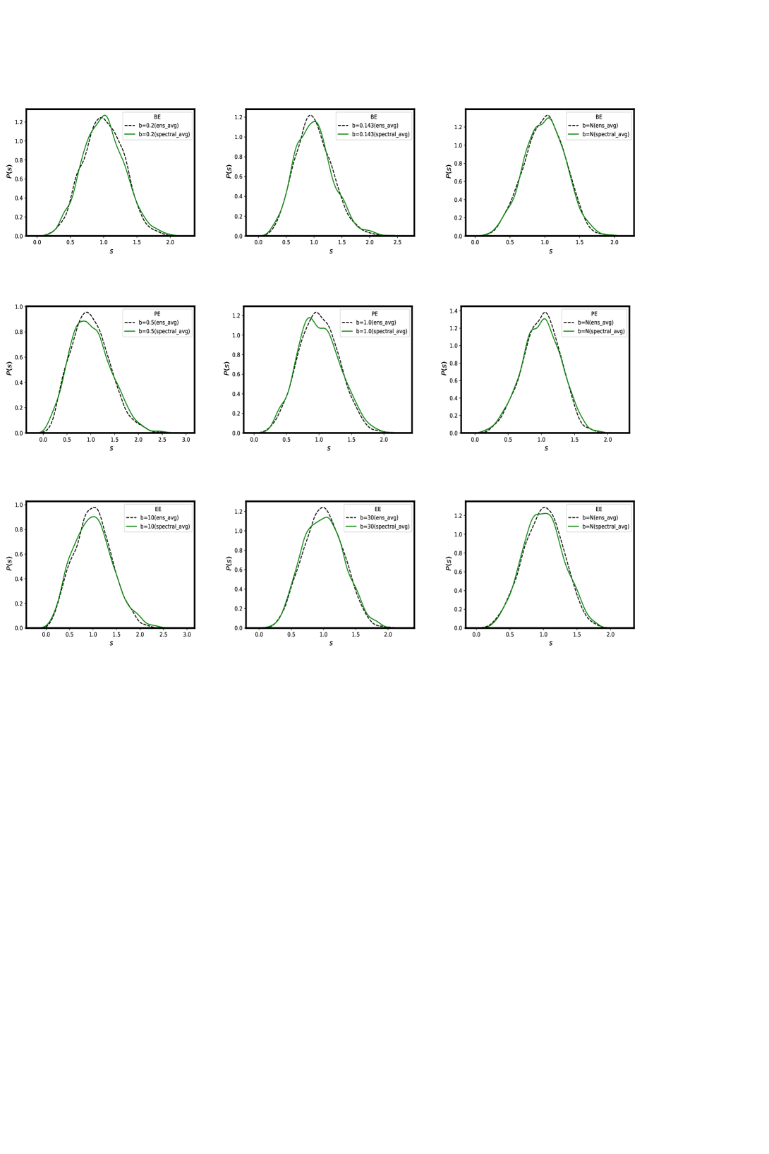
Figure 2: Non-Ergodicity of the spectral fluctuations on the complex plane: The figure displays a comparison of $P(S)$ obtained by ensemble averaging with that of spectral-ensemble averaging for three different $b$-values for each ensemble (i.e BE, PE and EE). The ensemble averaging is obtained by choosing a single spacing (equivalently at a single spectral point) near $z\sim 0$ and averaging over an ensemble of many matrices. The spectral-ensemble averaging is carried out by averaging over a few spacings from each matrix as well as over the ensemble. As the visuals indicate, the two averages are almost analogous as $b\sim N$.

Figure 1 displays a comparison of the $P(S,\Lambda_{e})$ distribution for $e\sim 0$ and three $b$-values (equivalently for three $\Lambda_{e}$ ), obtained by two different averaging approaches for each of the three ensembles. The first averaging route, referred as the ensemble averaging, is as follows: we first choose a single spacing from a matrix from the neighbourhood of $e=0$ and then study its distribution over an ensemble of ten matrices ($M=10$). The second route, based on both spectral as well as ensemble averaging and referred here as ”spectral-ensemble averaging” is as follows: we consider $10\%$ spacings around $e=0$ for each matrix in the ensemble, obtain their distribution for the matrix and then average it over the ensemble. The number of levels used in each case are also kept same to avoid non-physical deviations arising from e.g. finite size sample errors. While a slight deviation between the two averaging types is clearly visible from figure 1 for each of the three ensembles for $b\ll N$, it survives, albeit rather weakly, even for Ginibre limit ($b=N$ case) of each ensemble too. Theoretically however the Ginibre ensemble as well as its local fluctuations are expected to be stationary. This motivates us to attribute it to the observed deviation to finite sample error and interpret the illustrations in figure 1 as follows: the two types of averaging are almost in agreement for each ensemble, thereby suggesting the local ergodicity of the fluctuations. But the latter does not imply stationarity of the spectrum. This can further be illustrated by consideration of the Ginibre ensemble; as the latter’s spectrum is stationary, the distribution of $P(S,\infty)$ is expected to be independent of the location $"e"$ and is indeed confirmed in figure 2. In contrast, as indicated by our numerics, the deviation for BE, PE and EE are sensitive to the spectral location of the single spacing thus indicating non-stationarity of the spectrum (corresponding figure not included here).

III.3 Lack of Sensitivity to Multiple System Parameters: Emergence of Complexity Parameter

Contrary to stationary spectrum, the local correlations in our case are not translational or rotational invariant i.e vary on the complex spectral plane from one point to another for a fixed set of system conditions. A variation of the latter can change them even at a given spectral point ”$e$” too but, as discussed in section II, the change is governed by $\Lambda_{e}$, describing a collective influence of the system conditions and not their individual details.

Our previous study indicated an almost constant average level density in the bulk of the spectrum for each of the above ensembles. As this implies local stationarity of the fluctuations, one can consider levels within an optimized spectral range without mixing the statistics. We analyze 10${\%}$ of the total eigenvalues taken from a range $\Delta e$ centred at $e\sim 0$; his gives approximately $10^{5}$ eigenvalues for each ensemble which are unfolded by $R_{1,local}$ given by eq.(15). As the non-stationarity of the spectrum renders a definition of the long range spectral measure not very clear, here we consider two fluctuation measures, both indicators of short range spectral behavior.

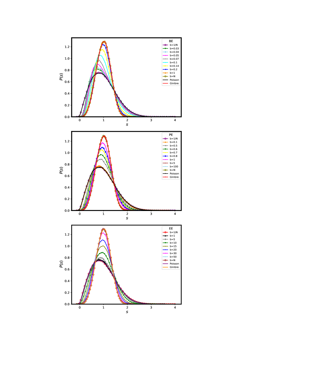
Figure 3: $P(S)$ for non-Hermitian ensembles: crossover from Poisson $\to$ Ginibre universality class: The figure displays the spectral-ensemble averaged nearest neighbour spacing distribution $P(s)$ of the eigenvalues on the complex plane for many $b$ values while $N$ is kept fixed ($N=1024)$ for the three ensembles., each consisting of 5000 matrices. As can be seen from the figure, a smooth crossover from Poisson to GInibre limit occurs for each case as $b$ varies. A good agreement of $P(S)$ for finite $\Lambda_{e}$ with eq.(16) is displayed in figure 4 (the comparison displayed in a separate figure for the purpose of clarity).

Spacing Distribution: Although at present no theoretical formulation is available for the $P(S,\Lambda_{e})$ intermediate between the above two extremes, its approximation by $R_{2}$ suggest, from eq.(8), a smooth crossover governed by the single parameter $\Lambda_{e}$. Thus the form of $P(S,\Lambda_{e})$ is expected to be intermediate between Poisson and Ginibre universality class (discussed in appendix A, eq.(18) and eq.(19)) if $\Lambda_{e}$ is a finite and non-zero. Figure 3 displays the $P(s,\Lambda_{e})$ behavior for each of the three ensembles for many $b$-values, equivalently many $\Lambda_{e}$ values obtained from eq.(7) along with eq.(14) and eq.(15). (We recall that the off-diagonal variances in PE and EE depend on additional system conditions manifesting through the difference of their decay types, mentioned in the beginning of section III.A). As clear from these figures, the statistics undergoes a crossover from Poisson to Ginibre statistics as $\Lambda_{e}$ varies. Although the mathematical form for $\Lambda_{e}$ is different for the three ensembles, and, its variation effectively implies variation of more than one system parameter for PE and EE (as clear from eq.(14), $P(S,\Lambda_{e})$ seems to evolve between two stationary limits in an analogous way for the three ensemble. This encourages us to conjecture

$$P(S,\Lambda_{e})=A\;S^{B}\;{\rm e}^{-C\;S^{2}}$$ (16)

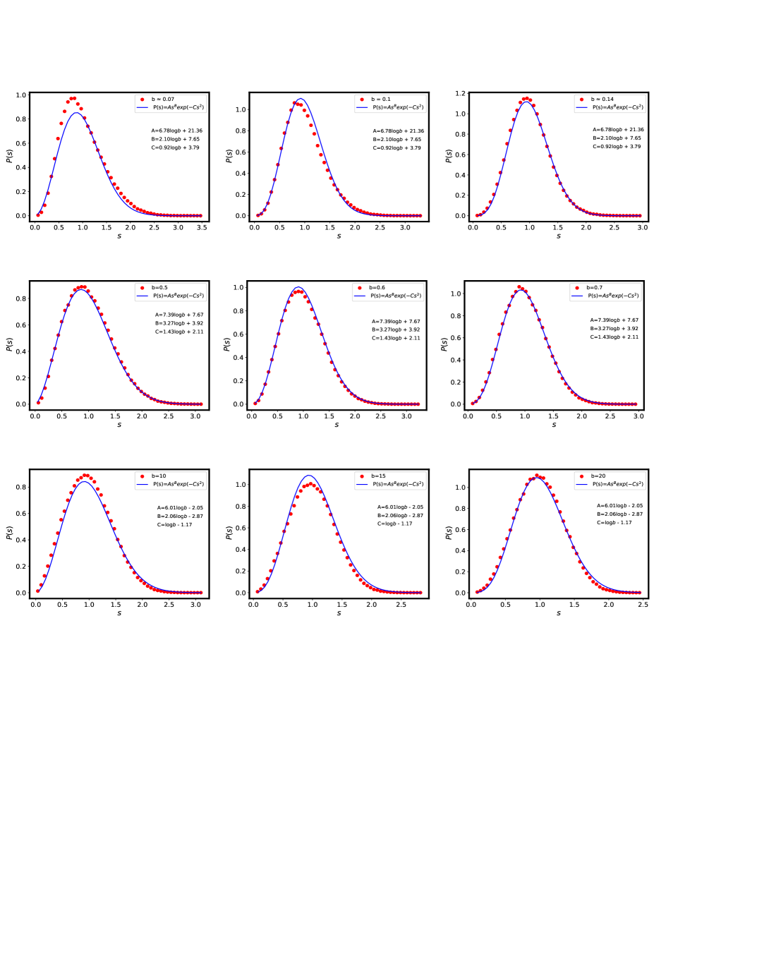
Figure 4: $P(S)$ for finite $\Lambda_{e}$: comparison with theoretical conjecture eq.(16): The figure displays a comparison with eq.(16) of the $P(S)$ many $b$ values and a fixed $N=1024$ for the three ensembles., each consisting of 5000 matrices. A lack of theoretical formulation of $P(S)$ in the intermediate regime motivates us to conjecture it by $P(S;\Lambda_{e})=AS^{B}\;{\rm exp}(-CS^{2})$ with $A,B,C$ as functions of $\Lambda_{e}.$ only Here again the definition $\Lambda_{e}=\log b-C$ as the crossover parameter seemingly apply quite well.

As displayed in figure 4, the good agreement of our numerical results with eq.(16) indeed supports the above conjecture. The numerical fit for the BE case, based on $N=1024$ and of an ensemble of $2500$ matrices, gives $A=6.78(\log b+3.15)$, $B=2.1(\log b+3.79)-0.31$, $C=0.92\log b+3.79$; this can be recast in the suggestive form $A\sim 6.78\Lambda_{e},B\sim 2.1\Lambda_{e},C\sim\Lambda_{e}$ using $\Lambda_{e}=\log b+3.79$. For PE case, the numerical fit gives $A=7.39(\log b+1.03)$, $B=3.27(\log b+1.2)$, $C=1.43(\log b+1.48)$, thereby suggesting $A\sim 7.39\Lambda_{e},B\sim 3.27\Lambda_{e},C\sim 1.43\Lambda_{e}$ with $\Lambda_{e}=\log b+1.48$. Simialrly for EE, we obtain $A=6.01(\log b-1.88)$, $B=2.06(\log b-1.17)-0.46$, $C=\log b-1.17$ thus suggesting $A\sim 6.01\Lambda_{e},B\sim 2.06\Lambda_{e},C=\Lambda_{e}$ with $\Lambda_{e}=\log b-1.17$.

Spacing Ratio Distribution:

As briefly discussed in appendix B, the unfolding related technical issues and errors can be avoided by consideration of the nearest neighbour spacing ratio, a dimensionless measure. With eigenvalues of a complex matrices distributed on a complex plane, a generalization of the spacing ratio measure, referred as the distribution of the complex spacing ratios, was introduced in [12] for non-Hermitian ensembles. A complex spacing ratio $Z_{k}$, defined as the ratio of the nearest neighbour spacing and next nearest neighbour spacing of a given eigenvalue $z_{k}$ on the complex plane $Z_{k}={z_{k}^{NN}-z_{k}\over z_{k}^{NNN}-z_{k}}$. The probability density $P(Z)$ of finding a spacing ratio $Z$ over an ensemble for a specific spectral range is then again free of unfolding issues and contains information not only about the radial correlations but the angular ones too. The latter can also be seen directly from the distribution of the radial and angular parts of the spacing ratio; writing $Z=r\;{\rm e}^{i\theta}$, we have $\rho_{\theta}(r)=\int{\rm d}\theta\;r\;P(Z)$ and $\rho_{r}(\theta)=\int{\rm d}r\;r\;P(Z)$.

For uncorrelated eigenvalues distributed on a complex plane, the spacing ratios are isotropic and consequently $\rho_{poi}(r)\propto\;r\;\Theta(1-r)$ [12]. No closed form expression for lage $N$ is however known for Ginibre ensemble of complex matrices (referred as GinUE in [12]). Although an exact result is obtained for $N=3$ in [12] but, contrary to Hermitian case, it is not a good approximation in large $N$ limit; (we recall that exact for $N=2$ for Hermitian matrices well approximates large $N$ behavior too). As discussed in [12], the leading order expansion in powers of $r$ in large $N$-limit yields $\rho_{gin}(r)\propto\;r^{3}$ valid only for spectral range around $r=0$. In the regime intermediate to Poisson and Ginibre ensemble, however, no theoretical results are currently available for $P(Z),\rho_{\theta}(r)$ or $\rho_{r}(\theta)$.

Figure 4 displays the behavior for $\rho_{\theta}(r)$ and $\rho_{r}(\theta)$ for the three ensembles in the bulk of the spectrum near $e\sim 0$ . Besides reconfirming the information contained in figure 3, i.e a smooth crossover from Poisson to Ginibre with increasing $b$ and thereby $\Lambda_{e}$ for each ensemble, it also indicates (i) an almost power law variation of $\rho(r)$ with $r$ for a fixed $\Lambda_{e}$, (ii) each ensemble has the same value of $\rho_{\theta}(r)$ at $r=0.5$ irrespective of $\Lambda_{e}$, thereby indicating $\Lambda_{e}$-insensitivity of $\rho_{\theta}(r)$ at $r=0.5$, (iii) rapid drop of $\rho_{r}(\theta)$ near $\theta=0$ as $\Lambda_{e}$ increases; clearly the drop occurs due to increasing level repulsion as $\Lambda$ increases. But, in comparison to $\rho_{\theta}(r)$, the variation is $\rho_{r}(\theta)$ with $\Lambda_{e}$ is more conspicuous; this indicates the important role played by angular correlations in the statistics. We also note that the case $\Lambda_{e}=0$ is indeed almost constant and is therefore in agreement with theoretical prediction for Poisson universality class (on complex plane).

III.4 Universality and Criticality in Spectral Statistics

Based on eq.(3), our theoretical claim is the following: different ensembles subjected to same global constraints are expected not only to undergo similar evolution of the spectral statistics but also to display same statistics if their $\Lambda_{e}$ values are same. It will be instructive to verify the claim for BE, PE and EE where, due to different variance structures, it is not at all obvious as to why their statistics be analogous for some specific set of system parameters. The theoretical predictions for the analogues for BE, PE and EE can be determined by invoking the condition $\Lambda_{e,BE}=\Lambda_{e,PE}=\Lambda_{e,EE}$, with $\Lambda_{e}$ given by eq.(14) and $R_{1,local}(e)$ for each case determined numerically from eq.(15). Here however we consider a more general route. To rule out that the analogy is not a mere coincidence and exist for other $\Lambda_{e}$ values too, we compare the three ensembles for full crossover of a fluctuation measure from $\Lambda_{e}=0\to\infty$. One traditionally used measure in this context is the cumulative nearest neighbour distribution $I(e,\Lambda_{e})=\int_{0}^{x}P(S,e;\Lambda_{e})\;{\rm d}s$ with $x$ as an arbitrary point. Alternatively, a related measure, particularly useful for phase transition studies, is the relative behavior of the tail of the nearest-neighbour spacing distribution $P(s)$, defined as

$$\gamma(x;\Lambda_{e})=\frac{I(x,\Lambda_{e})-I(x;\infty)}{I(x,0)-I(x,\infty)}$$ (17)

We choose $x$ as one of the two crossing points $x_{1},x_{2}$ of $P(S,\infty)=P_{g}(s)$ and $P(S,0)=P_{p}(s)$ (here the subscripts $g$ and $p$ refer to the Ginibre and Poisson cases respectively): $x_{1}=0.656978$ and $x_{2}=1.446259$. As obvious, $\gamma=0$ and $1$ for Ginibre and Poisson limit respectively and a fractional value of $\gamma$ indicates the probability of small-spacings different from the two limits. In limit $N\to\infty$, a $\gamma$ value different from the two end points is an indicator of a new universality class of statistics and therefore a critical point.

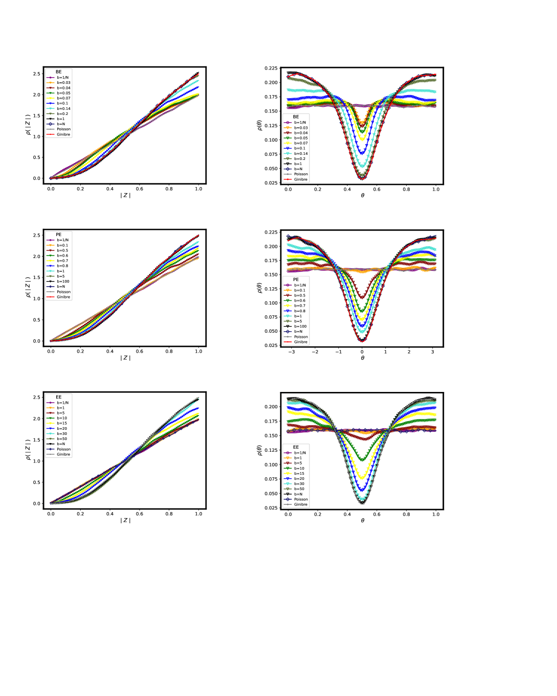
Figure 5: Radial and angular dependence of spacing ratios: Figure illustrates the radial $\rho(|z|)$ and angular parts $\rho(\theta)$ of the spectral-ensemble averaged nearest neighbour spacing distribution $P_{z}(z)$ with $z=|z|{\rm e}^{i\theta}$ on the complex plane for many $b$ values for fixed system size $N=1024$ and ensembles size $M=5000$. As shown in left panels of figure, $\rho(|z|)$ is almost independent of the ensemble parameter $b$, with $\rho(|z|)\approx 1$ at $|z|\approx 0.5$, for each ensemble. An increasing $\rho(|z|)$ with $|z|$ indicates level repulsion. The display in right panel confirm the almost homogeneous $\rho(\theta)$ distribution in Poisson limit for each ensemble but it rapidly changes with increasing $b$. Indeed $\rho(\theta)$ approaches a minimum for $\theta=0$ as $b$ approaches Ginibre limit. This indicates that increasing level repulsion among consecutive eigenvalues with increasing $b$ causes them to lie at large angular separations.

As $\Lambda_{e}$ determination for full range $0\to\infty$ requires a prior knowledge of analytical form of $R_{1,local}(e)$, here we consider the $\gamma$ behavior with respect to another parameter, namely, $\tau\equiv\log(b)-C$ with $C=0,1.8,4.6$ for BE, PE and EE respectively. We note that, from eq.(14), $\tau$ is directly related to $\Lambda_{e}$. Figure 5 shows a comparison of the variation of $\gamma_{1}$ and $\gamma_{2}$ with $\tau$, for two $x$-values and three ensembles for a fixed $N$; here $\gamma_{1}=\gamma(x_{1};\tau)$ and $\gamma_{2}=\gamma(x_{2};\tau)$, at the spectral point $e\sim 0$. The collapse of the $\gamma(x;\tau)$ behavior for each of the three ensemble onto a single curve confirms our theoretical claim regarding one parameter based universality of the local fluctuations. Figure 5 also shows a comparison, for three ensembles, of the variation of (i) $\langle\rho_{\theta}(r)\rangle_{r}$ and (ii) $\langle\rho_{r}(\theta)\rangle_{\theta}$. The good agreement for the three ensembles, of the two measures for entire crossover, once again confirms our theoretical claim regarding the single parameter dependence of the fluctuations. Further as the collapse of each fluctuation measure for the three ensembles occurs when plotted with respect to $\log(b)-c$; this again strongly suggests $\Lambda_{e}\propto\log(b)-c$. An important point worth emphasizing here is the following: while the three ensembles have different variance structures of the matrix elements, the point of inflection seems to be same in terms of $\log b-c$; this is again a confirmation of our claim about the existence of a single parametric formulation of the spectral statistics for Gaussian non hermitian ensembles.

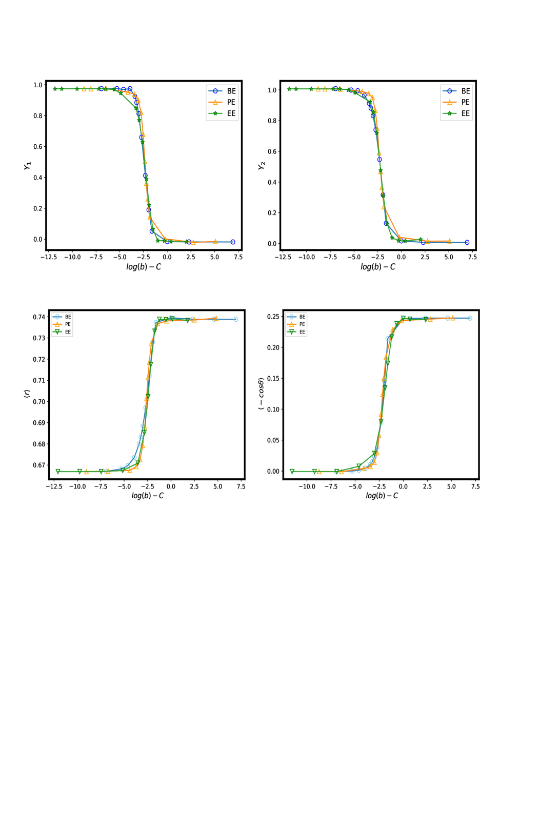
Figure 6: Universality of local fluctuations in non-stationary non hermitian ensembles: The figure displays the behavior of four different fluctuation measures, namely, $\gamma(x_{1}),\gamma(x_{2}),\rho_{\theta}(r),\rho_{r}(\theta)$ on the complex spectral plane, with $x_{1}=0.490658$ and $x_{2}=1.06205$. As can be seen from the figure, the behavior of each measure vs $\log b-c$ for three ensembles collapses onto same curve, with $c=0,1.8,4.6$ for BE, PE and EE respectively. An important point worth noting is the rapid transition of each measure from one extreme limit to another, indicating a critical statistics near $\log b-c\approx-2$.

The illustrations in figure 5 suggest another important aspect of the fluctuations, namely, the existence of a critical statistics: as $\log(b)$ increases, $\gamma_{1},\gamma_{2},\langle\rho_{\theta}(r)\rangle_{r}$ and $\langle\rho_{r}(\theta)\rangle_{\theta}$ undergo a rapid transition from Ginibre ($\gamma_{1,2}=1$) to Poisson limit ($\gamma_{1,2}=0$); this in turn suggests the existence of a critical statistics near $\log(b)-c\approx-2.5$. As mentioned in previous section, the spectral statistics at the critical point is, by definition, size-independent and is characterized by a size-independent $\Lambda_{e}$. To confirm the existence of a critical point, it is therefore necessary to analyze the size-dependence of the spectral measures at the critical $b$-values resulting in size-independent $\Lambda_{e}$. As displayed in figure 6, $P(S,\Lambda_{e})$ behavior for the BE case, with a $b$-value, arbitrarily chosen intermediate between Poisson and Ginibre limits, seems to be almost insensitive to system size $N$. This motivates us to consider the mesaures $\gamma_{1},\gamma_{2},\langle r\rangle,\langle\cos\theta\rangle$ for BE for many $b$-and $N$-values. As displayed in figure 6, the measures turn out to be size-independent for almost entire $b$-range, thus indicating the statistics as critical for arbitrary $b$ value, thereby implying ensemble in eq.(9) itself to be critical. We note that a similar criticality of the Brownian ensemble has already been reported for Hermitian cases [46].

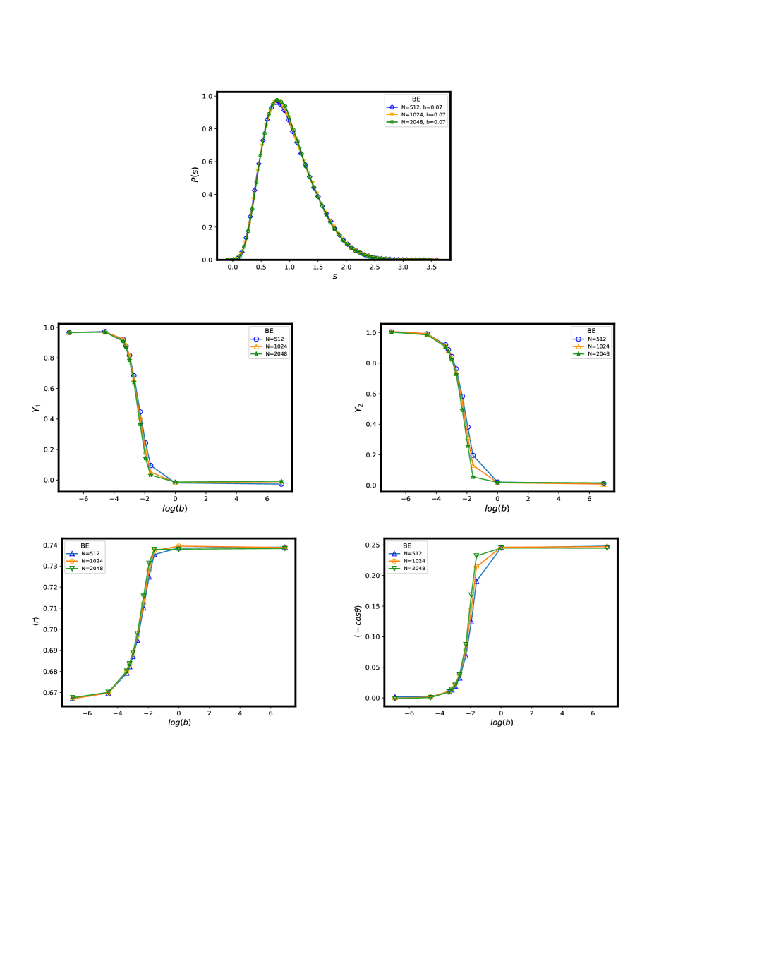
Figure 7: Critical BE Statistics The figure displays the statistical behavior for BE at critical values of the ensemble parameters (given in eq.(9)) based on following fluctuation measures: (i) $P(S)$, (ii) $\gamma_{1}$, (iii) $\gamma_{2}$, (iv) $\langle r\rangle$, (v) $\langle\cos\theta\rangle$. As can be seen from each parts of the figure, the statistics for each measure remains invariant with changing $N$ for entire range of $b$. This indicates the criticality of the ensemble for chosen set of the ensemble parameters. More clearly the spectral statistics near $e\sim 0$ is critical irrespective of the $b$ and $N$ values if the variances of the diagonal are taken in a specific combination described in eq.(9).

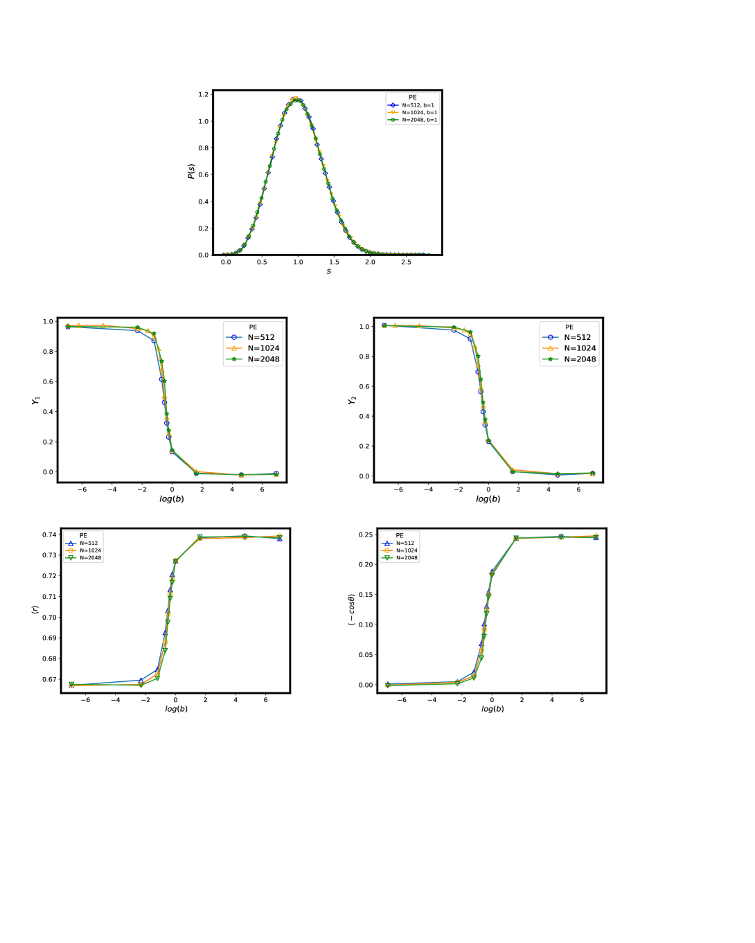
Figure 8: Critical PE Statistics: the details here are same as in figure 7 except now the critical PE ensemble is described by eq.(10).

Figures 7 and 8 display the corresponding behavior of the above measures for PE and EE case too. As in the BE case, here again the collapse of the curves for almost entire $b$-range and different $N$ values, for each of the measure, namely, $P(S,\Lambda_{e}),\gamma_{1},\gamma_{2},\langle r\rangle,\langle\cos\theta\rangle$, indicates the criticality of PE and EE with their distribution parameters given by eq.(10) and eq.(11). The results in figures 6-8 also reconfirm $\log b$ as the parameter governing the spectral statistics; this in turn strongly suggests $\Lambda_{e}$ as a function of $\log b-C$. A comparison with non-zero $C$ values in figure 5 thus suggest $C$ as a ensemble specific constant, independent of size $N$.

IV Conclusion

We numerically analyze various physical aspects e.g. ergodicity vs non-ergodicity, universality and criticality of the local spectral fluctuations for non-stationary complex random matrix ensembles representing non-Hermitian many body/ disordered Hamiltonians subjected to perturbation and away from equilibrium. Based on analysis of three prototypical, basis-dependent ensembles, subjected to same global connstraints but with their variance structure representing three different types of quantum correlations in underlying basis space, our results clearly reveal non-ergodic as well as non-stationary aspect of the correlations. This information is relevant not only for fundamental interests in such ensembles but also in context of quantum information, neural networks as well as the non-Hermitian many body localization e.g. whether or not a non-Hermitian system can achieve thermalization?

The most important insight of our analysis is as follows: notwithstanding different variance structures, we find that the spectral statistics for each ensemble undergoes an analogous crossover from Poisson to Ginibre universality class in terms of a single parameter $\Lambda_{e}$ and also numerically identify the latter. This indicates a universality in bulk spectral statistics underlying in non-equilibrium regime of non-Hermitian systems and is consistent with theoretical claims based on complexity parametric approach reported in [1]. A lack of theoretical formulations of measures handicaps us from a comparison of our numerical results with theory but indirect verification is given by analogy of evolving statistics, between two stationary limits, for each ensemble in terms of $\Lambda_{e}$ .

An important aspect of complexity parameter formulation for both Hermitian as well non-Hermitian ensembles is its role as the criteria to determine the critical spectral statistics. The present analysis confirms the validity of the criteria for complex matrix ensembles with critical spectral statistics appearing between Poisson and Ginibre universality classes at the system conditions that keep rescaled complexity parameter $\Lambda$ size-independent. As this occurs for specific combinations of system parameters, it existence is not always gauranteed for all ensemble types.

For a deeper insight in the complexity parameter based formulation of the complex systems, it is relevant to compare present results with those already known in the domain of conservative systems. In case of the latter undergoing localized to delocalized transition with changing system conditions e.g. disorder or many body interactions, the Hermitian ensembles representing them undergo a crossover/abrupt transition of spectral statistics from Poisson to one of the ten stationary universality classes. As confirmed by previous studies, the transition can be well-described by $\Lambda_{e}$, the spectral complexity parameter [41, 46]. Similar studies on Hermitian ensembles with additonal constraints e.g positive definiteness or column constraint have also indicated the existence of non-equilibrium universality classes of spectral statistics, characterized by $\Lambda_{e}$ [42, 47]. While the basic idea remains same as in Hermitian case, the nature of the universality classes in non-Hermitian cases is expected to be different. While we do have a clear understanding of the ensemble complexity parameter $Y$ for non-Hermitian cases, a theoretical formulation of $\Lambda_{e}$ is still missing. As in the Hermitian case, its technical definition is again expected to be dependent on eigenfunction correlation and therefore requires a detailed analysis of the latter.

Besides questions of eigenfunction fluctuations, our study gives rise to many other queries e.g. can the complexity parameter formulation be extended to non-Gaussian ensembles as well as to structured ensembles with correlated matrix elements? The information is relevant in order to model more generalized class of non-Hermitian systems e.g. neural networks where existence of additional matrix constraints can lead to many types of matrix elements correlations. For application to many body non-Hermitian systems it is relevant to analyze as to how the behavior of spectral correlations in the edge differ from the bulk? Another very important question, especially in context of toplogical mateials is the existence of exceptional points and their effect on the statistical behavior of the left and right eigenfunctions. The information is needed to understand e.g. the non-Hermitian skin effect [54] and the absence of conventional bulk-boundary correspondence in topological and localization transitions in non-Hermitian systems and also for applications to biological neural networks. We intend to answer some of the above queries in near future.

Appendix A Ergodicity of Ginbre ensemble

The ergodicity in a random matrix ensemble, consisting of replicas of some linear operator, implies an analogy of the spectral averages for one of its replica with those over the ensemble e.g as in the case of Ginibre ensemble. Indeed the ergodicity of the ensemble is a manifestation of its stationarity i.e basis invariance which permits the eigenfunctions to be ergodic. The stationarity of the spectrum however corresponds to an analogy of the local fluctuations at any two arbitrary spectral points equivalently, translational invariance in case of spectrum along a real line and both translational as well as rotational invariance in case of complex plane. This can further be illustrated by consideration of the Ginibre ensemble; as the latter’s spectrum is stationary, the distribution of $P(S,\infty)$ is expected to be independent of the location $"e"$ and is indeed confirmed in figure 1. The numerical study in [49] has already confirmed the ergodicity of the average spectral density in Ginibre limit.

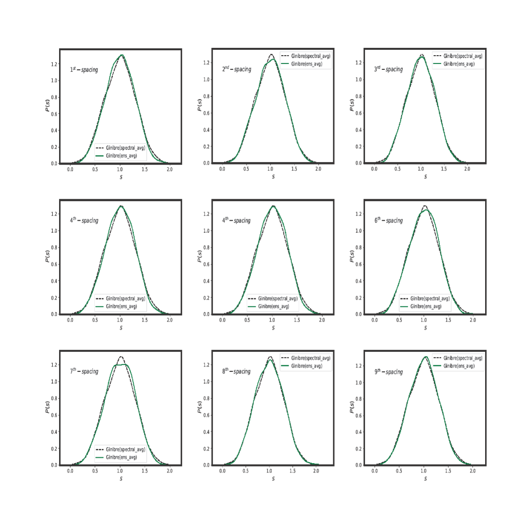
Figure 1: Ergodicity of the spectral fluctuations on the complex plane for Ginibre ensemble : The figure displays a comparison, for different choice of single spacings, of $P(s)$ obtained by ensemble averaging with that of spectral averaging. Contrary to the display in figure 1, here the two averages almost overlap in each case, irrespective of the choice of the single spacing used for the ensemble averaging.

Appendix B Nearest Neighbor Spacing Distribution (NNSD)

A nearest neighbor spacing $S_{1,k}$ for an unfolded eigenvalue $e_{k}$ is defined as $|e_{k}-e_{\alpha}|$ with $e_{\alpha}$ as the nearest eigenvalue to $e_{k}$ on the complex plane: $S_{1,k}=min_{\alpha}|e_{k}-e_{\alpha}|$. Due to ease of measurement, the spectral analysis through experimental as well as numerical route is often based on the distribution $P(S,e)$ of unfolded nearest neighbor spacings $S$ at spectral point $e$ and thus a measure for short range correlations. While $R_{2}(S;e)$ in general depends on the eigenvalue spacings $S$ of all orders, it is approximately same as $P(S;e)$ for small $S$. (Indeed, as in case of a real spectrum, ${\mathcal{R}}_{2}$ can be expressed as a sum over $k^{th}$ order spacing distributions $P_{k}(S;e)$: ${\mathcal{R}}_{2}(S,e)=\sum_{k=0}^{\infty}P_{k}(S,e)$ with $P_{0}\equiv P$ as the nearest neighbor spacing distribution [51]). Using the above relation in eq.(8) then implies that the evolution of $P_{k}(S,e)$ with changing system conditions and from an arbitrary initial condition is governed by $\Lambda_{e}$ too for all $k$ including $k=0$.

With changing system conditions, the eigenvalues distribution on a complex plane for many non-Hermitian systems undergoes a variation between two extremes, namely, uncorrelated eigenvalues (Poisson universality class) and correlated eigenvalues through mutual repulsion (Ginibre universality class). For the former, $P(S;e)$ is the 2-dimensional Poisson distribution, independent of $e$:

$$P(S)=2c_{p}S\;{\rm e}^{-\alpha_{p}\;S^{2}}$$ (18)

with $c_{p}$ and $\alpha_{p}$ determined from the normalization condition $\int_{0}^{\infty}P(S)\;{\rm d}S=1$ and the unit mean level spacing condition $\int_{0}^{\infty}S\,P(S)\;{\rm d}S=1$. For the Ginibre ensemble of complex matrices, the spacing distribution $P(S;e)$ (independent of $e$) is [13]:

$$P(S)=c_{g}\;P_{g}(c_{g}S)$$ (19)

with

$$P_{g}(S)=\lim_{N\to\infty}\left[\prod_{n=1}^{N-1}f_{n}(S^{2})\;{\rm e}^{-S^{2}}\right]\;\left[\sum_{n=1}^{N-1}\frac{2S^{2n+1}}{n!\;f_{n}(S^{2})}\right]$$ (20)

and

$$f_{n}(x)=\sum_{m=0}^{n}\frac{x^{m}}{m!}={\rm e}^{x}-\sum_{m=n+1}^{\infty}\frac{x^{m}}{m!}$$ (21)

and with $c_{g}$ as the mean level spacing $\int_{0}^{\infty}\;S\;P_{g}(S)\;{\rm d}S\approx 1.1429$.

From eq.(21), $f_{n}(x)$ for $S<1$ limit can be approximated as $f_{n}(x)\sim 1$. This in turn gives, for small-$S$, $P(S)=(1/2)\;c_{g}^{3}\;S^{3}\;{\rm e}^{-c_{g}^{2}\;S^{2}}$. For large $S(>1)$, $f_{n}(x)$ can be approximated by its dominant term $f_{n}(x)\sim\frac{x^{n}}{n!}$. This in turn gives the dominant contribution from the second bracket in eq.(20) as $S$ and from the first bracket as $\left(\prod_{n=1}^{N-1}\frac{S^{2n}}{n!}\right)\;{\rm e}^{-S^{2}}$. For $S>1$, eq.(20) can then be approximated as $P(S)\sim S\;\left(\prod_{n=1}^{N-1}\frac{c_{g}^{2n}\;S^{2n}}{n!}\right)\;{\rm e}^{-c_{g}^{2}\;S^{2}}$ or simply as $P(S)\sim\;{\rm e}^{-c_{g}^{2}\;S^{2}}$ (with exponential term domunating over powers of $S$).

Appendix C Spacing Ratio Distribution

For a meaningful comparison of the statistics of two different ensembles or even those for a same ensemble at two different spectral locations, it is necessary to rescale the spectrum by $R_{1,local}(e)$. This however requires a prior knowledge of $R_{1,local}(e)$ which is often not known for non-stationary ensembles and the standard route is to determine it through numerical calculation. Besides, in case $R_{1}(e)$ is not a smooth function of energy, the unfolding procedure becomes non-trivial even if $R_{1}(e)$ is analytically known and the spectrum is locally stationary. Indeed as almost all standard spectral fluctuation measures e.g nearest neighbour spacing distribution and number variance are sensitive to unfolding issues, it is preferable to consider a dimensionless measure e.g. the nearest neighbour spacing ratio. For real spectrum, the measure is defined as [55] $P(r)=\sum_{i=1}^{N-1}\langle\delta(r-r_{i})\rangle$ with $r$ defined as the ratio of consecutive spacings between nearest neighbour levels: $r_{i}=S_{i+1}/S_{i}$ where $S_{i}=e_{i+1}-e_{i}$ is the distance between two nearest neighbour eigenvalues. As the ratio $r$ does not depend on the local density of states, an unfolding of the spectrum for $P(r)$ is not required. Further $P(r)$ being a short range fluctuation measure, the probability of error due to mixing spectral statistics is reduced.

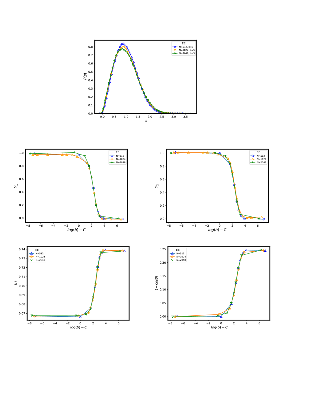
Figure 9: Critical EE Statistics: The details here are same as in figure 7 except now the critical EE ensemble is described by eq.(11).

References

- [1] P. Shukla, Phys. Rev. Lett. 87, 19, 194102, (2001).
- [2] M. V. Berry, Czechoslovak J.Phys. 54, 1039, (2004).
- [3] F.Haake et al., Z.Phys. B, 88, 359, (1992).
- [4] Y. Ashida, Z. Gong, and M. Ueda, Advances in Physics 69, 249 (2020).
- [5] Z. Gong, Y. Ashida, K. Kawabata, K. Takasan, S. Hi-gashikawa, and M. Ueda, Phys. Rev. X8, 031079 (2018).
- [6] A. amir, N. Hatano and D. R. Nelson, Phys. Rev. E 93, 042310, (2016).
- [7] Y. Ahmadian, F. Mumarola and K. D. Miller, Phys. Rev. E 91, 012820, (2015).
- [8] N.Moiseyev, Non-Hermitian Quantum Mechanics (Cambridge University Press, 2011).
- [9] Y. C. Hu and T. L. Hughes, Phys. Rev. B84, 153101 (2011).
- [10] H. Schomerus, Opt. Lett.38, 1912 (2013).
- [11] K. Ranjan and L. F. Abbott, Phys. Rev. Lett., 97, 188104, (2006).
- [12] L. Sa, P. Ribciro and T. Prosen, Phys. Rev. X, 10, 021019, (2020).
- [13] R. Hamazaki, K. Kawabata, N. Kura and M. Ueda, Phys. Rev. Res., 2, 023286, (2020).
- [14] O. Bohigas and M. P. Pato, J. Phys. A: Math. Theor. 46, 115001, (2013).
- [15] A. M. Garcia-Garicia, S. M. Nishigaki and J.J.M. Verbaarschot, Phys. Rev. E 66, 016132, (2002).
- [16] G.De Tomasi and I. Khaymovich, Phys. Rev. B, 106, 094204 (2022).
- [17] J. Feinberg and A. Zee, Phys. Rev. E59, 6433 (1999).
- [18] L. G. Molinari, Journal of Physics A: Mathematical and Theoretical 42, 265204 (2009).
- [19] Y. Huang and B. I. Shklovskii, Phys. Rev. B 101, 014204 (2020).
- [20] G. L. Celardo, M. Angeli, and R. Kaiser, arXiv preprint arXiv:1702.04506 (2017).
- [21] F. Cottier, A. Cipris, R. Bachelard, and R. Kaiser, Phys. Rev. Lett.123, 083401 (2019).
- [22] C. E. Maximo, N. A. Moreira, R. Kaiser, and R. Bachelard, Phys. Rev. A100, 063845 (2019).
- [23] C.M. Bender, N. Hassanpour, D.W.Hook, S.P.Klevansky, C. Sunderhauf and Z. Wen, Phys. Rev. A 95, (2017).
- [24] C.M. Bender and S. Boettcher, Phys. Rev. Lett. 80, 5243, (1998).
- [25] C.M. Bender, D.C. Brody and H.F.Jones, Phys. Rev. Lett. 89, (2002).
- [26] J. Feinberg and A.Zee, Phys. Rev. E 59, 6433, (1999)
- [27] Y.V.Fyodorov and H.-J. Sommers, J. Math. Physics (N.Y.), 38, 1918, (1997).
- [28] H.J.Sommers et al., Phys. Rev. Lett., 60, 1895 (1988).
- [29] N.Hatano and D.R.Nelson, Phys. Rev. Lett. 77, 570 (1996).
- [30] K.B.Efetov, Phys Rev. B 56, 9630 (1997).
- [31] I.Y.Glodsheild and B.A.Khoruzhenko, Phys. Rev. Lett., 80,2897 (1998).
- [32] C.Mudry, B.D.Simons and A.Altland, Phys. Rev. Lett., 80,4257 (1998).
- [33] J.T.Chalker and Z.J.Wang, Phys. Rev. Lett. 79, 1797, (1997).
- [34] D.R.Nelson and N.M.Shnerb, Cond-mat/9708071.
- [35] J.T.Chalker and B.Mehlig, Phys. Rev. Lett. 81, 3367, (1998).
- [36] Y.V.Fyodorov, B.A.Khoruzhenko and H.-J. Sommers, Phys. Rev. Lett., 79, 557, (1997).
- [37] Nils Lehmann and H-j Sommers, Phys. Rev. Lett. 67, 941, (1991).
- [38] Y.V.Fyodorov and B.A.Khoruzhenko, Ann. Inst. Henri Poincare (Physique Theorique), 68, 449, (1998).
- [39] F. Haake, Quantum Signatures of Chaos (Springer-Verlag, Berlin, 1991).
- [40] A.Pandey and P.Shukla, J. Phys. A: Math. Gen. , 24, 3907, (1991).
- [41] P.Shukla, Phys. Rev. E 62, 2098, (2000); J. Phys. A 41, 304023 (2008); Phys. Rev. E 71, 026266 (2005); Phys. Rev. E 75, 051113, (2007); J. Phys. A: Math. Theor 50, 435003 (2017); Phys. Rev. B, 98, 054206 (2018).
- [42] M. V. Berry and P.Shukla, J. Phys. A 42, 485102 (2009).
- [43] R. Dutta and P. Shukla,ibid. 76, 051124 (2007); 78, 031115 (2008).
- [44] Pragya Shukla, J. Phys. A: Math. Theor. 54 275001, (2021).
- [45] S. Sadhukhan and P. Shukla, Phys. Rev. E 96, 012109 (2017).
- [46] P. Shukla, New J. Phys. 18, 021004 (2016). .
- [47] T. Mondal and P.Shukla, Phys Rev. E 102, 032131 (2020)
- [48] P. shukla, Int. Jou. of Mod.Phys B (WSPC), 26, 12300008, (2012).
- [49] M. Gayas and P. Shukla, arXiv: (2023).
- [50] P. Shukla, J. Phys.: Condens. Matter 17, 1653 (2005).
- [51] J.B. French, V.K.B. Kota, A. Pandey and S. Tomsovic, Annals of Physics, 181, 198 (1988).
- [52] O. Bohigas and M. J. Giannoni, Ann. Phys. 89 422 (1975).
- [53] T A Brody, J Flores, J B French, P A Mello, A Pandey and S S M Wong Rev. Mod. Phys. 53 385 (1981).
- [54] N. Okuma, K. Kawabata, K. Shiozaki, and M. Sato, Phys.Rev. Lett.124, 086801 (2020).
- [55] Y Atas, E Bogomolny, O Giraud and G Roux, Phys. Rev. Lett. 110, 084101 (2013); V Oganesyan, A Pal and D A Huse, Phys. Rev. B 80, 115104 (2009); A Pal and D A Huse, Phys. Rev. B 82, 174411 (2010).