SPD-DDPM: Denoising Diffusion Probabilistic Models in the
Symmetric Positive Definite Space

Abstract

Symmetric positive definite (SPD) matrices have shown important value and applications in statistics and machine learning, such as FMRI analysis and traffic prediction. Previous works on SPD matrices mostly focus on discriminative models, where predictions are made directly on $E(X|y)$, where $y$ is a vector and $X$ is an SPD matrix. However, these methods are challenging to handle for large-scale data, as they need to access and process the whole data. In this paper, inspired by denoising diffusion probabilistic model (DDPM), we propose a novel generative model, termed SPD-DDPM, by introducing Gaussian distribution in the SPD space to estimate $E(X|y)$. Moreover, our model is able to estimate $p(X)$ unconditionally and flexibly without giving $y$. On the one hand, the model conditionally learns $p(X|y)$ and utilizes the mean of samples to obtain $E(X|y)$ as a prediction. On the other hand, the model unconditionally learns the probability distribution of the data $p(X)$ and generates samples that conform to this distribution. Furthermore, we propose a new SPD net which is much deeper than the previous networks and allows for the inclusion of conditional factors. Experiment results on toy data and real taxi data demonstrate that our models effectively fit the data distribution both unconditionally and unconditionally and provide accurate predictions.

Introduction

Symmetric positive definite (SPD) matrices hold significant importance within the domains of machine learning and multivariate statistical analysis. They play a pervasive role across a diverse range of applications, including FMRI analysis [33], hand gesture recognition  [25], facial recognition [28], traffic prediction [40], brain-computer interfaces [2], video classification [42; 15; 41], interaction recognition [24], and many more.

There are two main tasks for SPD matrices: classification and SPD matrix estimation. The first one involves using SPD matrices as inputs to predict the classes of matrices. They often involve transforming SPD matrices into Euclidean space vectors via a Log mapping and then employ SPDNet accompanied by convolution with activation [11] and batch normalization [3] for classification. Recently, several works have been proposed to modify SPD Net via multi-scale features, UNet structure, and local convolution [4; 41; 46]. The second one aims to estimate the SPD matrix as the predicted variable $X$. Previous methods often use traditional statistical modeling frameworks as discriminative models by estimating $E(X|y)$ given the conditional variables $y$. For example, they define an additive model in a reproducing kernel Hilbert space using kernel functions [20] or define a regression model in a metric space upon Fréchet mean [33; 34]. However, these models often face challenges when dealing with high-dimensional SPD matrices or predictor $y$. In addition, these methods primarily focus on predicting $E(X|y)$ and currently lack approaches for estimating the probability density in the SPD space. This motivates the construction of generative models for the SPD space. Such models not only benefit from predicting $p(X)$ but also utilize maximum likelihood estimation to make predictions for $X$ given conditional variables $y$.

Denoising diffusion probabilistic model (DDPM) [12] is one of the most popular and effective generative models. Several researchers have extended DDPM to Riemannian manifolds, including SO(3) [18], SE(3) [45], spheres [14], and more [6]. These extensions have proven to be of practical value in fields such as protein generation [5], molecular docking [5], and others. However, few works have discussed and studied the SPD space. Meanwhile, the classical DDPM has poor performance when estimating probability distribution in the SPD space. When real data resides on a low-dimensional manifold, estimating in a high-dimensional Euclidean space is inefficient, and the distribution on the manifold may not exhibit favorable characteristics in the Euclidean space where it is embedded.

To address the SPD space distribution estimation problem, we propose a novel denoising diffusion probabilistic model in the SPD space, termed SPD-DDPM. The key components of SPD-DDPM lie in the equation of the backward process and the network to generate SPD matrices. Firstly, by introducing Gaussian distribution, addition and multiplication operations in the SPD space, we extend the DDPM in the Eucidean space to the SPD space, including the forward and backward process. Secondly, we introduce a novel SPD net that takes an SPD matrix as input using double convolutions and allowing for the incorporation of conditions $y$ into the network.

Our contributions are summarized as follows:

• We propose a novel SPD-DDPM to accurately estimate the SPD matrix $X$, which provides two versions: conditional and unconditional generation.

• We introduce the Gaussian distribution in the SPD space, the addition and multiplication operations in the SPD space to extend the DDPM theory.

• A new SPD U-Net is proposed to effectively incorporate the conditions during the generative process.

Experiment results on toy data and real taxi data demonstrate that our models effectively fit the data distribution both unconditionally and unconditionally and provide accurate predictions.

Preliminary

Denoising Diffusion Probabilistic Model (DDPM)

Assume the source data $X$ is a distribution $X\sim q(X)$. DDPM defines a forward process of $T$ steps that gradually adds noise to transform the source data into a standard Gaussian distribution by:

$$q(X_{t}|X_{t-1})=N(\sqrt{1-\beta_{t}}X_{t-1},\beta_{t}I),$$ (1)

where $X_{t}$ is the forward output at the $t$-th step, and $\beta_{t}$ is a hyperparameter. Eq. 1 can be reparameterized as:

$$X_{t}=\sqrt{1-\beta_{t}}X_{t-1}+\sqrt{\beta_{t}}\epsilon_{t},\;\epsilon_{t}\sim N(0,I).$$ (2)

After that, we build the distribution of $q(X_{t}|X_{0})$ as:

$$\begin{split}q(X_{t}|X_{0})&=N(\sqrt{\bar{\alpha}_{t}}X_{0},(1-\sqrt{\bar{\alpha}_{t}})I),\\ \alpha_{t}&=1-\beta_{t},\,\bar{\alpha}_{t}=\prod_{i=0}^{t}\alpha_{i}.\end{split}$$ (3)

Note that the forward process does not require training. After $T$ forward steps, the source data $X$, a.k.a. $X_{0}$, is transformed into a normal distribution.

In the backward process, DDPM attempts to solve $q(X_{t-1}|X_{t},X_{0})$ based on Bayes theorem:

$$\begin{split}&q(X_{t-1}|X_{t},X_{0})=q(X_{t}|X_{t-1})\frac{q(X_{t-1}|X_{0})}{q(X_{t}|X_{0})}\\ &\qquad\qquad\qquad\quad=N(\mu_{t}(X_{t},X_{0}),\sigma^{2}_{t}I),\\ &\mu_{t}(X_{t},X_{0})=\frac{1}{\sqrt{\alpha_{t}}}(X_{t}-\frac{1-\alpha_{t}}{\sqrt{1-\bar{\alpha}_{t}}}\epsilon),\,\sigma_{t}^{2}=\frac{1-\bar{\alpha}_{t-1}}{1-\bar{\alpha}_{t}}\beta_{t}.\end{split}$$ (4)

where $\epsilon\sim N(0,I)$ represents the noise added to $X_{t}$, but we do not known its exact value when given $X_{t}$. Thus, a neural network $\epsilon_{\theta}$ is used to approximate it. The loss function can be formulated as:

$$\|\epsilon-\epsilon_{\theta}(X_{t},t)\|^{2}$$ (5)

According to Eq. 4, the reverse process is constructed to obtain $p(X_{t-1}|X_{t})$:

$$\begin{split}p(X_{t-1}|X_{t})&=N\big{(}\frac{1}{\sqrt{\alpha_{t}}}X_{t}-\frac{1-\alpha_{t}}{\sqrt{\alpha_{t}(1-\bar{\alpha}_{t})}}\epsilon_{\theta},\Sigma_{t}\big{)},\end{split}$$ (6)

where $\Sigma_{t}=\sigma_{t}^{2}I$.

During inference, the data $X_{T}$ is sampled from the standard Gaussian distribution and then employ Eq. 6 to gradually remove noise to generate the desired output of $\hat{X}$.

Symmetric Positive Definite (SPD) Space

Various real data (e.g., FRMI) are satisfied with the SPD condition to form SPD matrices, which is significantly different from the data in the Euclidean space. In the SPD space (denoted by $Sym^{+}$), symmetry and positive definiteness are held:

$$\begin{split}&Symmetry:\forall X\in Sym^{+},X^{{}^{\prime}}=X,\\ &Positive:\forall X\in Sym^{+},\forall a\in R^{m},a^{{}^{\prime}}Xa>0.\end{split}$$ (7)

Following [36], Gaussian distribution in the SPD space is defined as:

$$p(X|\bar{X},\sigma^{2})=\frac{1}{\zeta(\sigma)}\exp[-\frac{d(X,\bar{X})^{2}}{2\sigma^{2}}],$$ (8)

where $\zeta(\sigma)$ is the regularization coefficient. The distance $d$ in Eq. 8 is affine-invariant metric [23], which is defined as:

$$d(X_{1},X_{2})^{2}=tr[\log(X_{1}^{-0.5}X_{2}X_{1}^{-0.5})]^{2}.$$ (9)

Based on the above definition of affine-invariant metric, the exponent and logarithm mappings are formulated by following the work [11]:

$$\begin{split}\operatorname{Exp}_{X_{1}}(X_{2})&=X_{1}^{\frac{1}{2}}\exp(X_{1}^{-\frac{1}{2}}X_{2}X_{1}^{-\frac{1}{2}})X_{1}^{\frac{1}{2}},\\ \operatorname{Log}_{X_{1}}(X_{2})&=X_{1}^{\frac{1}{2}}\log(X_{1}^{-\frac{1}{2}}X_{2}X_{1}^{-\frac{1}{2}})X_{1}^{\frac{1}{2}}.\end{split}$$ (10)

In the SPD space, we can employ the exponent and logarithm mappings in Eq. 10 to further define the addition and multiplication operations in SPD space for computation:

In the SPD space, the base matrix we select is identity matrix $I$, and the addition operation $\oplus$ and multiplication operation $\odot$ can be defined as:

Definition 1

$$\begin{split}X_{1}\oplus X_{2}&=\operatorname{Exp}_{I}(\operatorname{Log}_{I}(X_{1})+\operatorname{Log}_{I}(X_{2})).\\ r\odot X&=\operatorname{Exp}_{I}(r\cdot\operatorname{Log}_{I}(X)).\end{split}$$ (11)

Since the base matrix $I$ used in Eq. 10, the exponent and logarithm mappings are equal to $\exp$ and $\log$ function. Thus, addition and multiplication operations in Definition  11 are reformulated as:

$$\begin{split}X_{1}\oplus X_{2}&=\exp(\log(X_{1})+\log(X_{2}))\\ &=\exp(\frac{1}{2}\log(X_{1})+\log(X_{2})+\frac{1}{2}\log(X_{1}))\\ &=\exp(\log(X_{1}^{\frac{1}{2}})+\log(X_{2})+\log(X_{1}^{\frac{1}{2}}))\\ &=\exp(\log(X_{1}^{\frac{1}{2}}X_{2}X_{1}^{\frac{1}{2}}))=X_{1}^{\frac{1}{2}}X_{2}X_{1}^{\frac{1}{2}},\end{split}$$ (12)

$$r\odot X=\exp(r\cdot\log(X))=\exp(\log(X^{r}))=X^{r}.$$ (13)

In the work [39], SPD space with affine-invariant metric is a homogeneous space under the action of the linear group $GL(m)$, where the group action is defined as:

$$(X,A)\rightarrow X\cdot A\overset{\underset{def}{}}{=}A^{{}^{\prime}}XA.$$ (14)

Therefore, the affine-invariant metric remains invariant under group actions:

$$d(X_{1},X_{2})^{2}=d(X_{1}\cdot A,X_{2}\cdot A)^{2}.$$ (15)

Based on Eqs.  15, 8, and  9, we have the following proposition:

Proposition 1

$X\sim G(\bar{X},\sigma^{2})\implies X\cdot A\sim G(\bar{X}\cdot A,\sigma^{2}).$

Proof:

For any function $f:P_{m}\rightarrow R$ ($P_{m}$ is SPD space), and any $A\in GL(m)$, according to Eq.14, we have:

$$\int_{P_{m}}f(X)dv(X)=\int_{P_{m}}f(X\cdot A)dv(X).$$

where $dv(X)$ is the Riemannian volume element defined as:

$$dv(X)=det(X)^{-\frac{m+1}{2}}\prod_{i\leq j}dX_{ij}.$$

Intuitively, $dv(X)$ is the Riemannian volume element of $ds^{2}(X)$, and $ds^{2}(X)$ is invariant under congruence transformations and inversion:

$$ds^{2}(X)=tr[X^{-1}dX]^{2}.$$

Let $X$ be a random variable in $P_{m}$, let $\phi:P_{m}\rightarrow R$ be a test function. If $X\sim G(\bar{X},\sigma^{2})$ and $Z=X\cdot A$, then the expection of $\phi(Z)$is given by:

$$\begin{split}&\int_{P_{m}}\phi(X\cdot A)p(X|\bar{X},\sigma^{2})dv(X)\\ &=\int_{P_{m}}\phi(Z)p(Z\cdot A^{-1}|\bar{X},\sigma^{2})dv(Z)\\ &=\int_{P_{m}}\phi(Z)p(Z|\bar{X}\cdot A,\sigma^{2})dv(Z).\end{split}$$

Method

Symmetric Positive Definite Denoising Diffusion Probabilistic Model (SDP-DDPM)

DDPM is computed under the Euclidean space, which can not directly be applied to the SPD space. To this end, we propose SDP-DDPM based on the operational rules (i.e., Eq. 12 and Eq. 13) and Proposition 1 in the SPD space.

In the forward process, following DDPM, we can formulate $q(X_{t}|X_{t-1})$ in the SPD space as:

$$q(X_{t}|X_{t-1})\sim G(\alpha_{t}\odot X_{t-1},\beta_{t}^{2}),$$ (16)

where $\alpha_{t}^{2}+\beta_{t}^{2}=1,$ and $G(\cdot,\cdot)$ is gaussian distribution in the SPD space defined in Eq. 8. By using Eq. 12, Eq. 13) and Proposition 1, we have:

$$\begin{split}X_{t}&=\alpha_{t}\odot X_{t-1}\oplus\beta_{t}\odot\epsilon_{t},\quad\epsilon_{t}\sim G(I,1)\\ &=X_{t-1}^{\frac{\alpha_{t}}{2}}\;\epsilon_{t}^{\beta_{t}}\;X_{t-1}^{\frac{\alpha_{t}}{2}}\\ &\sim G(\alpha_{t}\odot X_{t-1},\beta_{t}^{2}).\end{split}$$ (17)

By using Eq. 17, we can obtain the relationship between $X_{t}$ and $X_{0}$ as below:

$$\begin{split}X_{t}&=\alpha_{t}\odot X_{t-1}\oplus\beta_{t}\odot\epsilon_{t}\\ &=\alpha_{t}\odot(\alpha_{t-1}\odot X_{t-2}\oplus\beta_{t-1}\odot\epsilon_{t-1})\oplus\beta_{t}\odot\epsilon_{t}\\ &=\alpha_{t}\alpha_{t-1}\odot X_{t-2}\oplus\alpha_{t}\beta_{t-1}\odot\epsilon_{t-1}\oplus\beta_{t}\odot\epsilon_{t}\\ &=(\alpha_{t}\dots\alpha_{1})\odot X_{0}\oplus(\alpha_{t}\dots\alpha_{2})\beta_{1}\epsilon_{1}\oplus\dots\oplus\beta_{t}\epsilon_{t}\\ &=\bar{\alpha}_{t}\odot X_{0}\oplus\sqrt{1-\bar{\alpha}_{t}^{2}}\odot\epsilon,\;\epsilon\sim G(I,1)\\ &\sim G(\bar{\alpha}_{t}\odot X_{0},1-\bar{\alpha}_{t}^{2}),\;\bar{\alpha}_{t}=\prod_{i=0}^{t}\alpha_{i}.\end{split}$$ (18)

The detailed proof of Eq. 36 in the SPD space is provided in the supplementary materials.

By defining $\bar{\beta}_{t}$ to be $\sqrt{1-\bar{\alpha}_{t}^{2}}$, $X_{t}$ can be further formulated as:

$${X_{t}=\bar{\alpha}_{t}\odot X_{0}\oplus\bar{\beta}_{t}\odot\epsilon.}$$ (19)

Based on Eq. 19, we only set $\bar{\alpha}_{t}$ to approach 0, $X_{t}$ will be transformed to the standard Gaussian distribution in the SPD space. Empirically, $\alpha_{t}$ is set to $\sqrt{1-\frac{0.08t}{T}}$ in our experiments, such that $\bar{\alpha}_{t}\rightarrow{0}$ when $t\rightarrow\infty$. Therefore, we can randomly sample the noise from the standard Gaussian distribution in the SPD space, and use the following backward process to generate the desired output.

In the backward process, we also compute $q(X_{t-1}|X_{t},X_{0})$ using the Bayesian technique as:

$$\begin{split}&q(X_{t-1}|X_{t},X_{0})=q(X_{t}|X_{t-1})\frac{q(X_{t-1}|X_{0})}{q(X_{t}|X_{0})}\\ &\propto\exp(-\frac{d(X_{t},X_{t-1}^{\alpha_{t}})^{2}}{2\beta_{t}^{2}}-\frac{d(X_{t-1},X_{0}^{\bar{\alpha}_{t-1}})}{2\bar{\beta}_{t-1}^{2}})\\ &\propto\exp[-\frac{tr(\bar{\beta}_{t-1}^{2}\alpha_{t}^{2}+\beta_{t}^{2})(\log\tilde{\mu}^{-\frac{1}{2}}\,X_{0}\,\tilde{\mu}^{-\frac{1}{2}})^{2}}{2\bar{\beta}_{t-1}^{2}\beta_{t}^{2}}]\\ &\sim G(\tilde{\mu}(X_{0},\epsilon),\tilde{\sigma}_{t}^{2}),\\ &\mathrm{with}\quad\tilde{\mu}(x_{0},\epsilon)=\frac{1}{\alpha_{t}}\odot X_{t}\ominus\frac{\beta_{t}^{2}}{\alpha_{t}\bar{\beta}_{t}}\odot\epsilon,\tilde{\sigma}_{t}=\frac{\bar{\beta}_{t-1}\beta_{t}}{\bar{\beta}_{t}}.\end{split}$$ (20)

Note that the final computation expression of $q(X_{t-1}|X_{t},X_{0})$ is similar to DDPM (i.e., Eq. 4), while their difference is that our addition and scalar multiplication are defined through exponential and logarithmic mappings. In Euclidean space, the exponential and logarithmic mappings can be regarded as addition and subtraction operations.

Further, we also formulate $p(X_{t-1}|X_{t})$ as:

$${p(X_{t-1}|X_{t})\sim G(\mu_{\theta}(X_{t},t),\Sigma_{t}^{2})},$$ (21)

where $\Sigma_{t}^{2}=\beta_{t}^{2}$. $\mu_{\theta}(X_{t},t)$ can be computed according to $q(X_{t-1}|X_{t},X_{0})$:

$$\begin{split}\mu_{\theta}(X_{t},t)=\frac{1}{\alpha_{t}}\odot X_{t}\ominus\frac{\beta_{t}^{2}}{\alpha_{t}\bar{\beta}_{t}}\odot\epsilon_{\theta}.\end{split}$$ (22)

During training, we aim to minimize the KL divergence between $p(X_{t-1}|X_{t})$ and $q(X_{t-1}|X_{t},X_{0})$. We also found that $\operatorname{KL}(q(X_{t-1}|X_{t},X_{0})\parallel p(X_{t-1}|X_{t}))$ is bounded by $d(\mu_{X_{0},\epsilon},\mu_{\theta})^{2}$, i.e.,

$$\begin{split}&KL(q(X_{t-1}|X_{t},X_{0})\parallel p(X_{t-1}|X_{t}))\\ &\propto\frac{2\beta_{t}^{2}d(\mu_{\theta},X)^{2}-2\tilde{\sigma}_{t}^{2}d(\mu_{X_{0},\epsilon},X)}{2\beta_{t}^{2}\tilde{\sigma}_{t}^{2}}\\ &\propto\frac{2\beta_{t}^{2}[d(\mu_{\theta},X)^{2}-d(\mu_{x_{0},\epsilon},X)^{2}]}{2\beta_{t}^{2}\tilde{\sigma}_{t}^{2}}\\ &\leq\kappa\,d(\mu_{X_{0},\epsilon},\mu_{\theta})^{2},\end{split}$$ (23)

where $\kappa$ is a constant, and $d(\mu_{X_{0},\epsilon},\mu_{\theta})^{2}$ is further simplified as:

$$\begin{split}&d(\mu_{X_{0},\epsilon},\mu_{\theta})^{2}\\ &=d(\frac{1}{\alpha_{t}}\odot X_{t}\ominus\frac{\beta_{t}^{2}}{\alpha_{t}\bar{\beta}_{t}}\odot\epsilon,\,\frac{1}{\alpha_{t}}\odot X_{t}\ominus\frac{\beta_{t}^{2}}{\alpha_{t}\bar{\beta}_{t}}\odot\epsilon_{\theta})^{2}\\ &=d(X_{t}^{-\frac{1}{2\alpha_{t}}}\epsilon^{\frac{\beta_{t}^{2}}{\alpha_{t}\bar{\beta}_{t}}}X_{t}^{-\frac{1}{2\alpha_{t}}},X_{t}^{-\frac{1}{2\alpha_{t}}}\epsilon_{\theta}^{\frac{\beta_{t}^{2}}{\alpha_{t}\bar{\beta}_{t}}}X_{t}^{-\frac{1}{2\alpha_{t}}})^{2}\\ &=d(\epsilon^{\frac{\beta_{t}^{2}}{\alpha_{t}\bar{\beta}_{t}}},\epsilon_{\theta}^{\frac{\beta_{t}^{2}}{\alpha_{t}\bar{\beta}_{t}}})^{2}\\ &=(\frac{\beta_{t}^{2}}{\alpha_{t}\bar{\beta}_{t}})^{2}d(\epsilon,\epsilon_{\theta})^{2}.\end{split}$$ (24)

For computational simplicity, we use $d(\epsilon,\epsilon_{\theta})^{2}$ as the training objective function. If we degenerate it to the Euclidean space, it will be $L_{2}$ distance to train DDPM. The detailed training process of SPD-DDPM is presented in Alg. 1.

For inference, we start from the standard Gaussian distribution in SPD space and gradually denoise the sample to generate $\hat{X}_{0}$, whose process is presented in Alg. 2. $\gamma$ is used to balance the diversity and robustness. A smaller $\gamma$ leads to greater diversity in the generated matrix, but it may result in low quality. On the other hand, a larger $\gamma$ produces higher quality outputs, but with reduced diversity.

Alg. 1, and  2 present the unconditional training of SPD-DDPM, while our SPD-DDPM also works well under the conditional generation. In the following, we will first describe the Symmetric Positive Definite U-Net to fit $\epsilon$ and then propose the conditional process of SPD-DDPM.

Algorithm 1 Unconditional Training of SPD-DDPM.

1:  repeat

2:     $t\sim\text{Uniform}({1,\cdots,T})$

3:     $X_{0}\sim q(X_{0})$

4:     $\epsilon\sim G(I,1)$

5:     $X_{t}=\bar{\alpha}_{t}\odot X_{0}\oplus\bar{\beta}_{t}\odot\epsilon$

6:     Take gradient descent step on$\nabla_{\theta}\parallel\epsilon-\epsilon_{\theta}(X_{t},t)\parallel$

7:  until convergence

Algorithm 2 Unconditional Sampling of SPD-DDPM.

1:  $X_{T}\sim G(I,1)$

2:  for $t=T,\dots 1$ do

3:     $z\sim G(I,1)$

4:     $X_{t-1}=\frac{1}{\alpha_{t}}\odot(X_{t}\ominus\frac{\beta_{t}^{2}}{\bar{\beta}_{t}}\epsilon_{\theta})\oplus\tilde{\sigma_{t}}/\gamma\odot z$, where $\ominus$ is defined by using $-$ to replace $+$ in Eq. 11.

5:  end for

6:  return  $X_{0}$

The detailed proofs presented in this section can be found in the supplement.

Symmetric Positive Definite U-Net

In SPD-DDPM, a neural network $\epsilon_{\theta}$ takes an SPD matrix and time $t$ as the inputs to output an SPD matrix. Traditional U-Net in DDPM can not guarantee the symmetry and positive definiteness of the output.Huang et al. [15] proposed a simple SPD Net by defining the convolution and activation layers. However, the objective of this network framework is to transform the SPD matrix into a vector in Euclidean space, and this network has a limited capacity to fit $\epsilon$. Moreover, the above SPD Net can not incorporate the conditional factors $t$. It fails to adapt to the different distributions of $X_{t}$ at different moments.

In this paper, we propose a novel high-capacity SPD U-Net framework to estimate the SPD matrix.

$$X_{k}=f_{b}^{(k)}(X_{k-1};W_{k})=W_{k}X_{k-1}W_{k}^{{}^{\prime}},$$ (25)

$$X_{k}=f_{r}^{(k)}(X_{k-1})=U_{k-1}\max(\epsilon I,\Sigma_{k-1})U^{{}^{\prime}}_{k-1}.$$ (26)

Furthermore, we add the time factor $t$ by first putting it through an embedding layer following a shallow neural network to generate a matrix $E_{t}$. As shown in Fig. 1, we incorporate the time factor $t$ into the neural network using the following equation:

$$X_{k}=E_{t}X_{k-1}E_{t}^{{}^{\prime}}.$$ (27)

To better estimate the distribution of source data, we increase the network depth by adding double convolution as shown in Fig. 1. The SPD matrix passes through a convolution layer using 25 and then adds condition $t$ by 27. After that, we do activation using 26. We repeat the above computation operation once more as a basic unit, termed double convolution, which increases the network depth and enhances its fitting capability.

The overall framework of our network is shown in Fig. 2. The down convolution is defined as $W_{k}\in R^{d_{k}\times d_{k-1}}(d_{k}<d_{k-1})$. The up convolution is defined as filling the diagonal of the input matrix with $1$ to match the output size, and then performing convolution (25). The concatenation layer is defined as computing the mean of two layers.

Different from Wang et al. [42], our neural network is deeper and allows for conditional additions. Additionally, the objective of our network is not to reconstruct the input SPD matrix but to fit other SPD matrices instead. We will conduct ablation experiments to evaluate the effectiveness of each component.

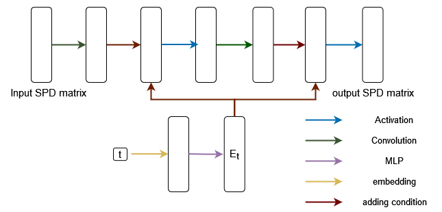
Figure 1: Double Convolution in SPD U-Net. Input matrix passes through convolution layers, followed by adding the condition of time factor $t$, and then activation layers. Repeat the above process making the double convolution block.

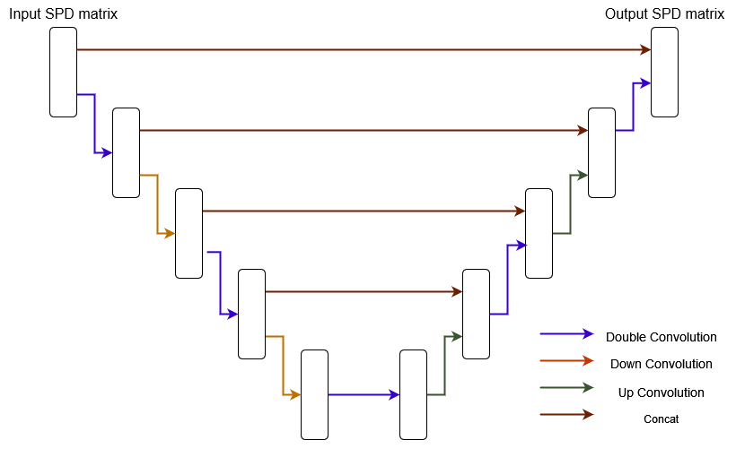
Figure 2: Architecture of SPD U-Net. SPD U-Net contains five double convolutions, two down convolution and two up convolution layers.

Conditional Symmetric Positive Definite Denoising Diffusion Probabilistic Model

We employ the classifier-free framework in the conditional generation, which additionally adds the conditional vector $y$ in the SPD net. Similar to the incorporation process of the time factor $t$, the conditional vector $t$ is transformed into a matrix via an embedding layer with a shallow network. Thus, the training loss function in the conditional SPD-DDPM can be formulated as:

$$\parallel\epsilon-\epsilon_{\theta}(X_{t},t,y)\parallel.$$ (28)

As presented in Alg. 3, the training process is similar to the unconditional SPD-DDPM.

In conditional generation, we aim to incorporate conditional generation as a novel approach for regression modeling. In regression models, it is common to assume that $X$ given $y$ follows a certain distribution and use $E(X|y)$ as the prediction of $X$ given $y$. In this work, we assume $X|y\sim G(\mu_{y},\sigma^{2})$ with $\mu_{y}$ being $E(X|y)$. Said et al. [36] have deduced that the maximum likelihood estimation of $E(X|y)$ is the empirical Riemannian centre of samples from $P(X|y)$, where the Riemannian centre $\hat{X}_{N}$ is defined as:

$$\hat{X}_{N}=\arg\min\limits_{X}\frac{1}{N}\mathop{\sum}\limits_{n=1}^{N}d(X,X^{n})^{2}.$$ (29)

$\hat{X}_{N}$ under the affine-invariant metric in Eq. 29 can be obtained using a gradient descent algorithm [8; 30; 32]. Therefore, we train the model to fit $p(X|y)$. During inference, given a specific $y$, we first generate $N$ samples from $p(X|y)$. We then compute $\hat{X}_{N}$ by minimizing Eq. (29) as the prediction of $E(X|y)$. The detailed inference process is presented in Alg. 4.

Algorithm 3 Conditional Training of SDP-DDPM.

1:  repeat

2:     $t\sim\text{Uniform}({1,\cdots,T})$

3:     $X_{0}\sim q(X_{0})$

4:     $\epsilon\sim G(I,1)$

5:     $X_{t}=\bar{\alpha}_{t}\odot X_{0}\oplus\bar{\beta}_{t}\odot\epsilon$

6:     Take gradient descent step on$\nabla_{\theta}\parallel\epsilon-\epsilon_{\theta}(X_{t},t,y)\parallel$

7:  until convergence

Algorithm 4 Conditional Inference of SDP-DDPM.

1:  for $i=1,\dots,N$ do

2:     $X_{T}^{i}\sim G(I,1)$

3:     for $t=T,\dots 1$ do

4:        $z\sim G(I,1)$

5:        $X_{t-1}^{i}=\frac{1}{\alpha_{t}}\odot(X_{t}^{i}\ominus\frac{\beta_{t}^{2}}{\bar{\beta}_{t}}\epsilon_{\theta})\oplus\tilde{\sigma_{t}}/\gamma\odot z$

6:     end for

7:  end for

8:  $\hat{X}=\arg\min\limits_{X}\frac{1}{N}\mathop{\sum}\limits_{n=1}^{N}d^{2}(X,X^{n})$

9:  return  $\hat{X}$

Experiments

Experimental Setups

Datasets. We use the simulation or toy data to test the performance of unconditional SPD-DDPM. We first randomly select a matrix $A$ as the center point of the distribution, and then sample total $15,000$ SPD matrices from $G(A,\sigma^{2})$ as the training data.

In the conditional generation, taxi data from the New York City Taxi and Limousine Commission is selected, which is available in Data preprocessing is following [40]. New York City is divided into $10$ boroughs (Detail refers to the supplementary materials). Each element of the SPD matrix $X_{ij}$ represents the passenger flow between the $i$-th borough and the $j$-th borough. We obtain $8,700$ weighted adjacency matrices by collecting data from 2019.1 to 2019.12 and also collect the $13$ predictors following [40]. We select $7,600$ samples as the training set and $1,100$ samples as the testing set.

Evaluation metric. In the unconditional generation, the Affine-invariant metric is widely used to test performance:

$$d(A,B)^{2}=tr[\operatorname{log}(A^{-0.5}BA^{-0.5})]^{2}.$$

In the condition generation, there is no previous method that optimizes under the Affine-invariant metric, so we select both Frobenius and Affine-invariant metric as the evaluation protocol, where Frobenius distance is defined as:

$$d(A,B)^{2}=\sqrt{\sum_{i=1}^{m}\sum_{j=1}^{m}(A_{ij}-B_{ij})^{2}}.$$

Implementation details. We implement our method using PyTorch 2.0.1 [29] with one NVIDIA A6000 GPU. The models are trained using Adam optimizer [17] with default parameters to DDPM. The learning rate is initialized by 0.0015 decaying by each iteration with the cosine function. The batch size is set to 150 and 100, and the total epochs are set to 50 and 20 in the unconditional and conditional generation, respectively. We set $\alpha_{t}$ and $T$ to $\sqrt{1-\frac{0.08t}{T}}$ and 200, respectively. $\gamma$ in Alg. 2 and  4 is both default set to 10 unless the specific discuss. Code is available at https://github.com/li-yun-chen/SPD-DDPM.

Unconditional Generation

We generate $300$ SPD matrices and use a heatmap to visualize the training samples and generated samples. Each heatplot shows the value of one SPD matrix. To evaluate the effectiveness of our unconditional SPD-DDPM, we compare our model with DDPM.

We first calculate the mean distance between the generated samples and the real distribution as a measure of evaluating the quality of generation. The results are summarized in Tab. 1. compared to DDPM, our unconditional SPD-DDPM achieves a lower mean distance. Furthermore, we visualize the generated samples in Fig. 3. Obviously, our models are better to fit the data, compared to DDPM. In this experiment, our data in the SPD space is a low-dimensional manifold, directly using DDPM to generate samples cannot be effective for the generation. In contrast, our unconditional SPD-DDPM fully considers the SPD information for better generation.

Table 1: Mean distance between the generated samples and the real distribution in the unconditional generation. $a\pm b$ means the mean and std in all tables by running the model 5 times, respectively.

Method	Mean Distance$\downarrow$
DDPM	813.75$\pm$ 187.92
SPD-DDPM	23.17$\pm$ 3.00

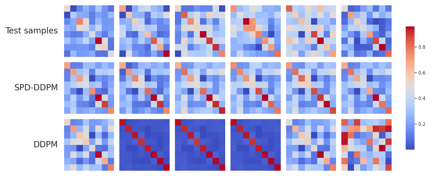
Figure 3: Visualization of SPD samples. We randomly select six samples from test samples, generated by SPD-DDPM and DDPM. Each column presents one sample.

Conditional Generation

Our goal is to use predictor variables $y$ to generate responding SPD matrices, achieving generative predictive modeling. Practically, we generate $n=20$ samples for each predictor $y$. We compare our method with the discriminative method Frechet Regression [33] and DDPM. Our method is optimized under the Affine-invariant metric, while Frechet Regression is optimized under the Forbinus metric. The results are summarized in Tab. 2. Our method outperforms Frechet Regression in both Frobenius and Affine-invariant metrics. In the Frobenius metric, our method slightly outperforms Frechet Regression because it is optimized under the Frobenius norm. In the Affine-invariant metric, our method significantly outperforms Frechet Regression. Our conditional SPD-DDPM also achieves significantly lower Frobenius metric, compared to DDPM.

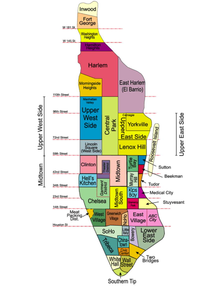
Figure 5: Towns in Manhattan, New York.

To further evaluate the effectiveness of our method, we visualize the SPD matrices in the Manhattan map Fig. 5. The left visualization represents the Frechet Regression, followed by the visualizations for our method and real data. We found that the predictions of Frechet Regression are overestimated and fail to capture the differences between each edge effectively. While our method shows a closer approximation to the real matrix.

Actually, discriminative methods require inputting all the data into the model simultaneously, rather than training in batches. When dealing with large-scale data, it will exceed memory limitations. Furthermore, their approach lacks the capability to retain intermediate model parameters, necessitating retraining the model when new samples need estimation. Our approach is based on the neural network, allowing us to circumvent the issues mentioned above.

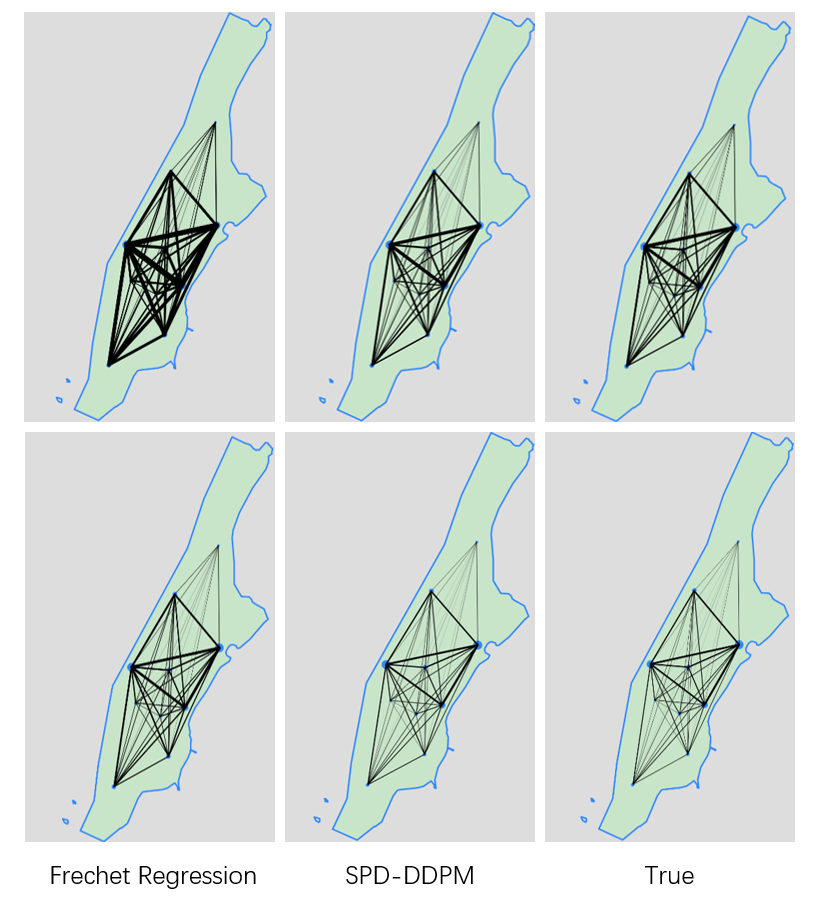
Figure 4: Visualization of taxi data. On the left is the data predicted by Frechet Regression, in the middle is the data predicted by our method, and on the right is the real data. Each node represents a region, and the thickness of the line segments represents the number of taxis.

Table 2: Comparsion among Frechet Regression, DDPM and SPD-DDPM for conditional generation.

Method	Frobenius $\downarrow$	Affine-invariant $\downarrow$
Frechet Regression	6.6448	8.0099
DDPM	62.97	1203.10
SPD-DDPM	6.4684	0.6123

Ablation Study

In this ablation study, we mainly evaluate the effects of hyperparameter $\gamma$ and SPD U-Net, which are very important to SPD-DDPM.

Effect of $\gamma$. We evaluate the effect of $\gamma$ in unconditional generation. As shown in Tab. 3, larger $\gamma$ generates a lower mean distance to better estimate the inputs. In addition, the std is also reduced by increasing $\gamma$.

Table 3: Effect of $\gamma$ for unconditional generation.

Method	Mean Distance$\downarrow$
SPD-DDPM($\gamma$ = 2)	65.81$\pm$ 17.86
SPD-DDPM($\gamma$ = 4)	35.99$\pm$ 7.58
SPD-DDPM($\gamma$ = 10)	23.17$\pm$ 3.00

Effect of SPD U-Net. In this paper, we propose a high-capacity SPD U-Net. Compared to the traditional SPD net, the network proposed in this paper is deeper and incorporates a double convolution, down and up convolution, and concatenation structure. We further demonstrate the effectiveness of these modifications through ablation experiments in unconditional generation by comparing the mean distance between samples and the distribution mean under $\gamma=10$.

Table 4: Ablation Study of SPD U-Net.

Method	Mean distance$\downarrow$
Without double convolution	26.17$\pm$ 3.75
Without concatenation	–
Without down&up convolution	42.75$\pm$ 3.25
SPD-DDPM with SPD U-Net	23.17$\pm$ 3.00

If we replace the double convolution with a single layer, reducing the number of convolutional layers by half, the performance of model generation decreases 3 mean distance. It indicates the effectiveness of double convolution for network’s fitting capability. The generation will fails when removing the concatenation structure. Thus, concatenation operations play a vital role in our SPD U-Net. Removing the down and up convolutions, each layer uses the matrices with the same dimensions, and the distance will increase to $42.75$, which significantly affects the model’s generalization ability.

Related Work

Denoising diffusion probabilistic model

DDPM is a generative model proposed by Ho et al. [12]. Nichol et al. [27] and Song et al. [37] further made improvements to it. Dhariwal et al. [7] proposed the classifier-guidance version, while Ho et al. [13] proposed the classifier-free version. The diffusion model is first applied in computer vision and found numerous applications in conditional image generation [26; 35], image restoration [43; 22], 3D image generation [44], and other fields. Song et al. [38] introduced the score-based generation method to accelerate the generation speed of the diffusion model from the perspective of stochastic differential equations [21]. Different with these methods, our SPD-DDPM is constructed on the SPD space, rather than Euclidean space. By introducing Gaussian distribution, the addition and multiplication operations in the SPD space, we effectively generate the forward and backward processes in the SPD space for better estimating the SPD matrix unconditionally and conditionally.

Symmetric positive definite metric

SPD space is a nonlinear metric space. Depending on the metric, SPD forms a Riemannian manifold. Different matrices have been proposed, such as affine-invariant metric [23; 31; 9], log-Euclidean metric [1], log-Cholesky metric [19] and scaling rotation distance [16]. Some work studied regression with SPD matrix valued responses. Using Frechet mean [10], Petersen et al. [33] proposed Frechet Regression under different matric. Based on this, Tucker et al. [40] proposed a method for variable selection. Lin et al. [20] proposed an adaptive model in SPD space. Qiu et al. [34] propose random forest with SPD matrix response. Different from these methods, our SPD-DDPM is the first generation model in SPD space, which can fit probability distribution in SPD space.

Conclusion

This paper proposes a novel denoising diffusion probabilistic model in the SPD space, termed SDP-DDPM. The proposed SDP-DDPM is applied for both unconditional and conditional generation. In the unconditional version, SDP-DDPM fits the probability distribution and generates samples in SPD space. In the conditional version, the model generates the distribution of SPD given a specific condition and calculates the expectation $E(X|y)$ as the prediction. A high-capacity SPD U-Net structure is further introduced to improve the data fitting performance. Experimental results demonstrate the strong capability of the proposed method in the fitting probability distributions.

Operations in the SPD Space

In this section, we will derive some operational properties in the SPD space, which will help us deduce properties of SPD-DDPM.

Distributive Law of Multiplication

Suppose $a$ is a scale, $X,Y$ are SPD matrices. Then

$$a\odot(X\oplus Y)=a\odot X\oplus a\odot Y.$$ (30)

Proof:

$$\begin{split}a\odot(X\oplus Y)&=a\odot\exp(\log X+\log Y)\\ &=\exp[a\cdot\log(\exp(\log X+\log Y))]\\ &=\exp[a\cdot(\log X+\log Y)]\\ &=\exp[a\log X+a\log Y]\\ &=\exp\{\log[\exp(a\log X)]+\log[\exp(a\log Y)]\}\\ &=\exp(a\log X)\oplus\exp(a\log Y)\\ &=a\odot X\oplus a\odot Y.\end{split}$$

Combining Similar Terms

Suppose $a,b$ is a scale, $X$ is an SPD matrix. Then

$$a\odot X\oplus b\odot X=(a+b)\odot X.$$ (31)

Proof:

$$\begin{split}&a\odot X\oplus b\odot X\\ &=\exp(a\log X)\oplus\exp(b\log X)\\ &=\exp\{\log[\exp(a\log X)]+\log[\exp(b\log X)]\}\\ &=\exp[a\log X+b\log X]\\ &=\exp[(a+b)\log X]\\ &=(a+b)\odot X.\end{split}$$

Multiplication of Gaussian Distribution in the SPD Space

Suppose $a$ is a scale, $\epsilon\sim G(I,\sigma^{2})$, Then

$$a\odot\epsilon\sim G(I,a^{2}\sigma^{2}).$$ (32)

Proof:

$d(\epsilon^{a},I)^{2}=tr[\log\epsilon^{a}]^{2}=tr[a\log\epsilon]^{2}=a^{2}tr[\log\epsilon]^{2}$

$$\begin{split}P(d(\epsilon^{a},I)^{2}<a^{2})&=P(d(\epsilon,I)^{2}<(\frac{r}{a})^{2})\\ &=\frac{\int_{0}^{\frac{r^{2}}{a^{2}}}e^{-\frac{u}{\sigma_{t}^{2}}}\,du}{\int_{0}^{\inf}e^{-\frac{u}{\sigma^{2}}}\,dz}\\ &=\frac{\int_{0}^{r^{2}}e^{-\frac{j}{\sigma^{2}a^{2}}}\,dj}{\int_{0}^{\inf}e^{-\frac{z}{\sigma^{2}a^{2}}}\,dz}\\ &\sim G(I,a^{2}\sigma^{2}).\end{split}$$

Constant Plus of Gaussian Distribution in the SPD Space

Suppose $Y$ is a constant SPD matrix, $\epsilon\sim G(I,\sigma^{2})$. Then

$$smallY\oplus\epsilon\sim G(Y,\sigma^{2}).$$ (33)

Proof:

$$\begin{split}Y\oplus\epsilon&=\exp[\log Y+\log\epsilon]\\ &=\exp[\frac{1}{2}\log Y+\log\epsilon+\frac{1}{2}\log Y]\\ &=\exp[\log(Y^{\frac{1}{2}}\,\epsilon\,Y^{\frac{1}{2}})]\\ &=Y^{\frac{1}{2}}\,\epsilon\,Y^{\frac{1}{2}}\\ &\sim G(Y,\sigma^{2}).\end{split}$$

Plus of Gaussian Distribution in the SPD Space

Suppose $\epsilon_{1}\sim G(I,\sigma_{1}^{2})$, $\epsilon_{2}\sim G(I,\sigma_{2}^{2})$. Then

$$small\epsilon_{1}\oplus\epsilon_{2}\sim G(I,\sigma_{1}^{2}+\sigma_{2}^{2}).$$ (34)

Proof:

Define $Z=\epsilon_{1}\oplus\epsilon_{2}$

$$\begin{split}&P(Z=a)\\ &=\int_{P_{m}}p(\epsilon_{1}=b)p(\epsilon_{2}=a\ominus b)\,dv(b)\\ &=\int_{P_{m}}\frac{1}{\zeta(\sigma_{1})}\frac{1}{\zeta(\sigma_{2})}\exp[-\frac{d(I,b)^{2}}{2\sigma_{1}^{2}}-\frac{d(I,a\ominus b)^{2}}{2\sigma_{2}^{2}}]\,dv(b)\\ &=\int_{P_{m}}\frac{1}{\zeta(\sigma_{1})}\frac{1}{\zeta({\sigma_{2}})}\exp[\\ &\qquad-\frac{(\sigma_{1}^{2}+\sigma_{2}^{2})tr[\log B]^{2}}{2\sigma_{1}^{2}\sigma_{2}^{2}}\\ &\qquad+\frac{2\sigma_{1}^{2}tr[\log a\log b]-\sigma_{1}^{2}tr[\log a]^{2}}{2\sigma_{1}^{2}\sigma_{2}^{2}}]\,dv(b)\\ &=\int_{P_{m}}\frac{1}{\zeta(\sigma_{1})}\frac{1}{\zeta({\sigma_{2}})}\exp[\\ &\qquad-\frac{tr[\sqrt{\sigma_{1}^{2}+\sigma_{2}^{2}}\log b-\frac{\sigma_{1}^{2}}{\sqrt{\sigma_{1}^{2}+\sigma_{2}^{2}}}\log a]^{2}}{2\sigma_{1}^{2}\sigma_{2}^{2}}\\ &\qquad+\frac{[\sigma_{1}^{2}-\frac{\sigma_{1}^{4}}{\sigma_{1}^{2}+\sigma_{1}^{2}}]tr[\log a]^{2}}{2\sigma_{1}^{2}\sigma_{2}^{2}}]\,dv(b)\\ &=\exp[-\frac{1-\frac{\sigma_{1}^{2}}{\sigma_{1}^{2}+\sigma_{2}^{2}}}{2\sigma_{2}^{2}}tr[\log a]^{2}]\frac{1}{\zeta(\sigma_{1})}\frac{1}{\zeta(\sigma_{2})}\\ &\qquad\int_{P_{m}}\exp[-\frac{tr[\sqrt{\sigma_{1}^{2}+\sigma_{2}^{2}}\log b-\frac{\sigma_{1}}{\sqrt{\sigma_{1}^{2}+\sigma_{2}^{2}}}\log a]^{2}}{2\sigma_{1}^{2}\sigma_{2}^{2}}]dv(b)\\ &\propto\,\exp[-\frac{d(I,a)^{2}}{2(\sigma_{1}^{2}+\sigma_{2}^{2})}].\end{split}$$

Distance of matrix power

Suppose $a$ is a scale, $X$ and $Y$ are SPD matrices. Then

$$d(X^{a},Y^{a})^{2}=a^{2}\,d(X,Y)^{2}.$$ (35)

Proof:

$$\begin{split}d(X^{a},Y^{a})^{2}&=tr[\log X^{-\frac{a}{2}}B^{a}Y^{-\frac{a}{2}}]^{2}\\ &=tr[-\frac{a}{2}\log X\oplus a\log Y\oplus-\frac{a}{2}\log X]^{2}\\ &=a^{2}tr[-\frac{1}{2}\log X\oplus\log Y\oplus-\frac{1}{2}\log X]^{2}\\ &=a^{2}tr[\log X^{-\frac{1}{2}}YX^{-\frac{1a}{2}}]^{2}\\ &=a^{2}\,d(X,Y)^{2}.\end{split}$$

Reparameterization of $q(X_{t}|X_{0})$

If $q(X_{t}|X_{t-1})\sim G(\alpha_{t}\odot X_{t-1},\beta_{t}^{2})$, $X_{t}$ can be written as:

$$small\begin{split}X_{t}=\alpha_{t}\odot X_{t-1}\oplus\beta_{t}\odot\epsilon_{t},\;\epsilon_{t}\sim G(I,1).\end{split}$$

This is further promoted as:

$$\begin{split}X_{t}&=\alpha_{t}\odot X_{t-1}\oplus\beta_{t}\odot\epsilon_{t}\\ &=\alpha_{t}\odot(\alpha_{t-1}\odot X_{t-2}\oplus\beta_{t-1}\epsilon_{t-1})\oplus\beta_{t}\odot\epsilon_{t}\\ &=\alpha_{t}\alpha_{t-1}\odot X_{t-2}\oplus\alpha_{t}\beta_{t-1}\odot\epsilon_{t-1}\oplus\beta_{t}\odot\epsilon_{t}\quad\mathrm{follow}\;\eqref{distribute law}\\ &=(\alpha_{t}\dots\alpha_{1})\odot X_{0}\oplus(\alpha_{t}\dots\alpha_{2})\beta_{1}\epsilon_{1}\oplus\dots\oplus\beta_{t}\epsilon_{t}\\ &=\bar{\alpha}_{t}\odot X_{0}\oplus\sqrt{1-\bar{\alpha}_{t}^{2}}\odot\bar{\epsilon}_{t},\,\bar{\epsilon}_{t}\sim G(I,1)\quad\mathrm{follow}\;\eqref{plus of gussian distribution}\\ &\sim G(\bar{\alpha}_{t}\odot X_{0},1-\bar{\alpha}_{t}^{2}).\quad\mathrm{follow}\;\eqref{constant plus}\eqref{multiplication}\end{split}$$ (36)

Computation of $q(X_{t-1}|X_{t},X_{0})$

$$\begin{split}&q(X_{t}|X_{t-1},X_{0})\\ &=q(X_{t}|X_{t-1})\frac{q(X_{t-1}|X_{0})}{q(X_{t}|X_{0})}\\ &=G(\alpha_{t}\odot X_{t-1},\beta_{t})\frac{G(\bar{\alpha}_{t-1}\odot X_{0},\bar{\beta}_{t-1})}{G(\bar{\alpha}_{t}\odot x_{0},\bar{\beta}_{t})}\\ &=\frac{\zeta(\bar{\beta}_{t})}{\zeta(\beta_{t})\zeta(\bar{\beta}_{t-1})}\exp(-\frac{d(X_{t},X_{t-1}^{\alpha_{t}})^{2}}{2\beta_{t}^{2}}\\ &\qquad-\frac{d(X_{t-1},x_{0}^{\bar{\alpha}_{t-1}})}{2\bar{\beta}_{t-1}^{2}}+\frac{d(X_{t},x_{0}^{\bar{\alpha}_{t}})}{2\bar{\beta}_{t^{2}}})\\ &\propto\exp(-\frac{d(X_{t},X_{t-1}^{\alpha_{t}})^{2}}{2\beta_{t}^{2}}-\frac{d(X_{t-1},X_{0}^{\bar{\alpha}_{t-1}})}{2\bar{\beta}_{t-1}^{2}})\\ &=\exp(-\frac{\bar{\beta}_{t-1}^{2}d(X_{t},X_{t-1}^{\alpha_{t}})^{2}+\beta_{t}^{2}d(X_{t-1},X_{0}^{\bar{\alpha}_{t-1}})}{2\beta_{t}^{2}\bar{\beta}_{t-1}^{2}})\\ &=\exp(-\frac{\bar{\beta}_{t-1}tr[\log(X_{t}^{-\frac{1}{2}}X_{t-1}^{\alpha_{t}}X_{t}^{-\frac{1}{2}})]^{2}}{2\beta_{t}^{2}\bar{\beta}_{t-1}^{2}}-\\ &\qquad\frac{\beta_{t}^{2}tr[\log(X_{0}^{-\frac{\bar{\alpha}_{t-1}}{2}}X_{t-1}X_{0}^{-\frac{\bar{\alpha}_{t-1}}{2}})]^{2}}{2\beta_{t}^{2}\bar{\beta}_{t-1}^{2}})\\ &=\exp(\frac{tr[\bar{\beta}_{t-1}^{2}\log(X_{t}^{-\frac{1}{2}}X_{t-1}^{\alpha_{t}}X_{t}^{-\frac{1}{2}})}{2\beta_{t}^{2}\bar{\beta}_{t-1}^{2}}-\\ &\qquad\frac{\beta_{t}^{2}\log(X_{0}^{-\frac{\bar{\alpha}_{t-1}}{2}}X_{t-1}X_{0}^{-\frac{\bar{\alpha}_{t-1}}{2}})]^{2}}{2\beta_{t}^{2}\bar{\beta}_{t-1}^{2}}).\end{split}$$

Translate $A=X_{t}^{-\frac{1}{2}}$ ,$B=X_{t-1}$, $C=X_{0}^{-\frac{\bar{\alpha}_{t-1}}{2}}$, $a=\bar{\beta}_{t-1}$, $b=\beta_{t}$, $r=\alpha_{t}$.

Then the numerator is written as:

$$\begin{split}&a^{2}(\log AB^{r}A)^{2}+b^{2}(\log CBC)^{2}\\ &=a^{2}(\log A+\log B^{r}+\log A)^{2}\\ &\qquad+b^{2}(\log C+\log B+\log C)^{2}\\ &=4a^{2}(\log A)^{2}+a^{2}(\log B^{r})^{2}+2a^{2}\log A\log B^{r}\\ &\qquad+2a^{2}\log B^{r}\log A+4b^{2}(\log C)^{2}+b^{2}(\log B)^{2}\\ &\qquad+2b^{2}\log C\log B+2b^{2}\log B\log C\\ &=(a^{2}r^{2}+b^{2})(\log B)^{2}+2(a^{2}r\log A+b^{2}\log C)\log B\\ &\quad+2\log B(a^{2}r\log A+b^{2}\log C)+4a^{2}(\log A)^{2}+4b^{2}(\log C)^{2}\\ &=(a^{2}r^{2}+b^{2})[(\log B)^{2}+2\frac{a^{2}r\log A+b^{2}\log C}{a^{2}r^{2}+b^{2}}\log B\\ &\quad+2\log B\frac{a^{2}r\log A+b^{2}\log C}{a^{2}r^{2}+b^{2}}]+4a^{2}(\log A)^{2}+4b^{2}(\log C)^{2}\\ &\propto(a^{2}r^{2}+b^{2})(\log D+\log B+\log D)^{2},\\ &\qquad\log D=\frac{a^{2}r\log A+b^{2}\log C}{a^{2}r^{2}+b^{2}}\\ &=(a^{2}r^{2}+b^{2})(\log DBD)^{2},\\ &\qquad D=A^{\frac{a^{2}r}{2(a^{2}r^{2}+b^{2})}}C^{\frac{b^{2}}{a^{2}r^{2}+b^{2}}}A^{\frac{a^{2}r}{2(a^{2}r^{2}+b^{2})}}.\end{split}$$ (37)

Thus $q(X_{t-1}|X_{t},X_{0})$ is written as:

$$\begin{split}&q(X_{t-1}|X_{t},X_{0})\\ &\propto\exp[-\frac{tr(a^{2}r^{2}+b^{2})(\log DBD)^{2}}{2\bar{\beta}_{t-1}^{2}\beta_{t}^{2}}]\\ &=\exp[-\frac{tr[\log DBD]^{2}}{2\frac{\bar{\beta}_{t-1}^{2}\beta_{t}^{2}}{a^{2}r^{2}+b^{2}}}]\\ &\sim G(\mu_{t},\tilde{\sigma}_{t-1}^{2}),\\ &\tilde{\sigma}_{t-1}^{2}=\frac{\bar{\beta}_{t-1}^{2}\beta_{t}^{2}}{a^{2}r^{2}+b^{2}}=\frac{\bar{\beta}_{t-1}^{2}\beta_{t}^{2}}{\bar{\beta}_{t-1}^{2}\alpha_{t}^{2}+\beta_{t}^{2}}=\frac{\bar{\beta}_{t-1}^{2}\beta_{t}^{2}}{\bar{\beta}_{t}^{2}},\end{split}$$ (38)

$$\begin{split}\mu_{t}&=D^{-2}\\ &=A^{-\frac{a^{2}r}{2(a^{2}r^{2}+b)}}C^{-\frac{b}{2^{2}(a^{2}r^{2}+b)}}A^{-\frac{a^{2}r}{2(a^{2}r^{2}+b)}}\\ &\quad C^{-\frac{b}{2^{2}(a^{2}r^{2}+b)}}A^{-\frac{a^{2}r}{2(a^{2}r^{2}+b)}}\\ &=X_{t}^{\frac{\bar{\beta}_{t-1}^{2}\alpha_{t}}{4(\alpha_{t}^{2}\bar{\beta}^{2}_{t-1}+\beta_{t}^{2})}}X_{0}^{\frac{\bar{\alpha}_{t-1}\beta_{t}^{2}}{2(\alpha_{t}^{2}\bar{\beta}^{2}_{t-1}+\beta_{t}^{2})}}X_{t}^{\frac{\bar{\beta}_{t-1}^{2}\alpha_{t}}{4(\alpha_{t}^{2}\bar{\beta}^{2}_{t-1}+\beta_{t}^{2})}}\\ &\quad X_{0}^{\frac{\bar{\alpha}_{t-1}\beta_{t}^{2}}{2(\alpha_{t}^{2}\bar{\beta}^{2}_{t-1}+\beta_{t}^{2})}}X_{t}^{\frac{\bar{\beta}_{t-1}^{2}\alpha_{t}}{4(\alpha_{t}^{2}\bar{\beta}^{2}_{t-1}+\beta_{t}^{2})}}\\ &=\frac{\bar{\beta}_{t-1}^{2}\alpha_{t}}{(\alpha_{t}^{2}\bar{\beta}^{2}_{t-1}+\beta_{t}^{2})}\odot X_{t}\oplus\frac{\bar{\alpha}_{t-1}\beta_{t}^{2}}{(\alpha_{t}^{2}\bar{\beta}^{2}_{t-1}+\beta_{t}^{2})}\odot X_{0}\\ &=\frac{\bar{\beta}_{t-1}^{2}\alpha_{t}}{(\alpha_{t}^{2}\bar{\beta}^{2}_{t-1}+\beta_{t}^{2})}\odot X_{t}\\ &\quad\oplus\frac{\bar{\alpha}_{t-1}\beta_{t}^{2}}{(\alpha_{t}^{2}\bar{\beta}^{2}_{t-1}+\beta_{t}^{2})}\odot[\frac{1}{\bar{\alpha}_{t}}(X_{t}\ominus\sqrt{\alpha_{t}^{2}\bar{\beta}^{2}_{t-1}+\beta_{t}^{2}}\epsilon_{t}]\\ &=\frac{\beta_{t}^{2}+\alpha_{t}^{2}\bar{\beta}^{2}_{t-1}}{\alpha_{t}(\alpha_{t}^{2}\bar{\beta}_{t-1}^{2}+\beta_{t}^{2})}\odot X_{t}\ominus\frac{\beta_{t}^{2}}{\alpha_{t}\sqrt{\alpha_{t}^{2}\bar{\beta}_{t-1}^{2}+\beta_{t}^{2}}}\odot\epsilon_{t}\\ &=\frac{1}{\alpha_{t}}\odot X_{t}\ominus\frac{\beta_{t}^{2}}{\alpha_{t}\bar{\beta}_{t}}\odot\epsilon_{t}.\end{split}$$

Upper Bound of KL divergence

Suppose

$$\begin{split}&q(X)\sim G(\mu_{1},\sigma_{1}^{2})\\ &p(X)\sim G(\mu_{2},\sigma_{2}^{2}).\end{split}$$

Then their KL divergence is bounded by:

$$\begin{split}&KL(q(X)\parallel p(X))\\ &\propto\frac{2\sigma_{1}^{2}d(\mu_{2},X)^{2}-2\sigma_{2}^{2}d(\mu_{1},X)}{2\sigma_{1}^{2}\sigma_{2}^{2}}\\ &\propto\frac{2\sigma_{1}^{2}[d(\mu_{2},X)^{2}-d(\mu_{1},X)^{2}]}{2\sigma_{1}^{2}\sigma_{2}^{2}}\\ &\leq\kappa\,d(\mu_{1},\mu_{2})^{2},\end{split}$$ (39)

where $\kappa$ is a constant.

Addition material for taxi data

Predictor

The predictior in experiment condition SPD-DDPM are as follows.

• Distance: Mean distance traveled, standardized

• Fare: Mean fare, standardized

• Passengers: Mean number of passengers, standardized

• Cash: Sum of cash indicators for type of payment, standardized

• Credit: Sum of credit indicators for type of payment, standardized

• Dispute: Sum of dispute indicators for type of payment, standardized

• Free: Sum of free indicators for type of payment, standardized

• Late Hour: Indicator for the hour being between 11pm and 5am, standardized

• average temperature

• average humidity

• average windspeed

• average pressure

• precipitation

Division of NewYork

In condition generation, Manhattan is divided into 10 zones, the division is described in Tab. 5

Table 5: 10 zones in Manhattan defined for the New York taxi data analysis

Zone	Town
1	Inwood, Fort George, Washington Heights,
	Hamilton Heights, Harlem, East Harlem
2	Upper West Side, Morningside Heights, Central Park
3	Yorkville, Lenox Hill, Upper East Side
4	Lincoln Square, Clinton, Chelsea, Hell’s Kitchen
5	Garment District, Theatre District
6	Midtown
7	Midtown South
8	Turtle Bay, Murray Hill, Kips Bay, Gramercy Park,
	Sutton, Tudor, Medical City, Stuy Town
9	Meat packing district, Greenwich Village,
	West Village, Soho, Little Italy, China Town,
	Civic Center, Noho
10	Lower East Side, East Village, ABD Park,
	Bowery, Two Bridges, Southern tip, White Hall,
	Tribecca, Wall Street

References

- Arsigny et al. [2007] Arsigny, V.; Fillard, P.; Pennec, X.; and Ayache, N. 2007. Geometric means in a novel vector space structure on symmetric positive-definite matrices. SIAM journal on matrix analysis and applications, 29(1): 328–347.
- Barachant et al. [2013] Barachant, A.; Bonnet, S.; Congedo, M.; and Jutten, C. 2013. Classification of covariance matrices using a Riemannian-based kernel for BCI applications. Neurocomputing, 112: 172–178.
- Brooks et al. [2019] Brooks, D.; Schwander, O.; Barbaresco, F.; Schneider, J.-Y.; and Cord, M. 2019. Riemannian batch normalization for SPD neural networks. Advances in Neural Information Processing Systems, 32.
- Chen et al. [2023] Chen, Z.; Xu, T.; Wu, X.-J.; Wang, R.; Huang, Z.; and Kittler, J. 2023. Riemannian Local Mechanism for SPD Neural Networks. In Proceedings of the AAAI Conference on Artificial Intelligence, volume 37, 7104–7112.
- Corso et al. [2022] Corso, G.; Stärk, H.; Jing, B.; Barzilay, R.; and Jaakkola, T. 2022. Diffdock: Diffusion steps, twists, and turns for molecular docking. arXiv preprint arXiv:2210.01776.
- De Bortoli et al. [2022] De Bortoli, V.; Mathieu, E.; Hutchinson, M.; Thornton, J.; Teh, Y. W.; and Doucet, A. 2022. Riemannian score-based generative modelling. Advances in Neural Information Processing Systems, 35: 2406–2422.
- Dhariwal and Nichol [2021] Dhariwal, P.; and Nichol, A. 2021. Diffusion models beat gans on image synthesis. Advances in neural information processing systems, 34: 8780–8794.
- Dryden, Koloydenko, and Zhou [2009] Dryden, I. L.; Koloydenko, A.; and Zhou, D. 2009. Non-Euclidean statistics for covariance matrices, with applications to diffusion tensor imaging.
- Fletcher and Joshi [2007] Fletcher, P. T.; and Joshi, S. 2007. Riemannian geometry for the statistical analysis of diffusion tensor data. Signal Processing, 87(2): 250–262.
- Fréchet [1948] Fréchet, M. 1948. Les éléments aléatoires de nature quelconque dans un espace distancié. In Annales de l’institut Henri Poincaré, volume 10, 215–310.
- Higham [2008] Higham, N. J. 2008. Functions of matrices: theory and computation. SIAM.
- Ho, Jain, and Abbeel [2020] Ho, J.; Jain, A.; and Abbeel, P. 2020. Denoising diffusion probabilistic models. Advances in neural information processing systems, 33: 6840–6851.
- Ho and Salimans [2022] Ho, J.; and Salimans, T. 2022. Classifier-free diffusion guidance. arXiv preprint arXiv:2207.12598.
- Huang et al. [2022] Huang, C.-W.; Aghajohari, M.; Bose, J.; Panangaden, P.; and Courville, A. C. 2022. Riemannian diffusion models. Advances in Neural Information Processing Systems, 35: 2750–2761.
- Huang and Van Gool [2017] Huang, Z.; and Van Gool, L. 2017. A riemannian network for spd matrix learning. In Proceedings of the AAAI conference on artificial intelligence, volume 31.
- Jung, Schwartzman, and Groisser [2015] Jung, S.; Schwartzman, A.; and Groisser, D. 2015. Scaling-rotation distance and interpolation of symmetric positive-definite matrices. SIAM Journal on Matrix Analysis and Applications, 36(3): 1180–1201.
- Kingma and Ba [2014] Kingma, D. P.; and Ba, J. 2014. Adam: A method for stochastic optimization. arXiv preprint arXiv:1412.6980.
- Leach et al. [2022] Leach, A.; Schmon, S. M.; Degiacomi, M. T.; and Willcocks, C. G. 2022. Denoising diffusion probabilistic models on so (3) for rotational alignment. In ICLR 2022 Workshop on Geometrical and Topological Representation Learning.
- Lin [2019] Lin, Z. 2019. Riemannian geometry of symmetric positive definite matrices via Cholesky decomposition. SIAM Journal on Matrix Analysis and Applications, 40(4): 1353–1370.
- Lin, Müller, and Park [2023] Lin, Z.; Müller, H.-G.; and Park, B. 2023. Additive models for symmetric positive-definite matrices and Lie groups. Biometrika, 110(2): 361–379.
- Lu et al. [2022] Lu, C.; Zhou, Y.; Bao, F.; Chen, J.; Li, C.; and Zhu, J. 2022. Dpm-solver: A fast ode solver for diffusion probabilistic model sampling in around 10 steps. Advances in Neural Information Processing Systems, 35: 5775–5787.
- Lugmayr et al. [2022] Lugmayr, A.; Danelljan, M.; Romero, A.; Yu, F.; Timofte, R.; and Van Gool, L. 2022. Repaint: Inpainting using denoising diffusion probabilistic models. In Proceedings of the IEEE/CVF Conference on Computer Vision and Pattern Recognition, 11461–11471.
- Moakher [2005] Moakher, M. 2005. A differential geometric approach to the geometric mean of symmetric positive-definite matrices. SIAM journal on matrix analysis and applications, 26(3): 735–747.
- Nguyen [2021] Nguyen, X. S. 2021. Geomnet: A neural network based on riemannian geometries of spd matrix space and cholesky space for 3d skeleton-based interaction recognition. In Proceedings of the IEEE/CVF International Conference on Computer Vision, 13379–13389.
- Nguyen et al. [2019] Nguyen, X. S.; Brun, L.; Lézoray, O.; and Bougleux, S. 2019. A neural network based on SPD manifold learning for skeleton-based hand gesture recognition. In Proceedings of the IEEE/CVF Conference on Computer Vision and Pattern Recognition, 12036–12045.
- Nichol et al. [2021] Nichol, A.; Dhariwal, P.; Ramesh, A.; Shyam, P.; Mishkin, P.; McGrew, B.; Sutskever, I.; and Chen, M. 2021. Glide: Towards photorealistic image generation and editing with text-guided diffusion models. arXiv preprint arXiv:2112.10741.
- Nichol and Dhariwal [2021] Nichol, A. Q.; and Dhariwal, P. 2021. Improved denoising diffusion probabilistic models. In International Conference on Machine Learning, 8162–8171. PMLR.
- Otberdout et al. [2019] Otberdout, N.; Kacem, A.; Daoudi, M.; Ballihi, L.; and Berretti, S. 2019. Automatic analysis of facial expressions based on deep covariance trajectories. IEEE transactions on neural networks and learning systems, 31(10): 3892–3905.
- Paszke et al. [2017] Paszke, A.; Gross, S.; Chintala, S.; Chanan, G.; Yang, E.; DeVito, Z.; Lin, Z.; Desmaison, A.; Antiga, L.; and Lerer, A. 2017. Automatic differentiation in pytorch.
- Pennec [1999] Pennec, X. 1999. Probabilities and statistics on Riemannian manifolds: Basic tools for geometric measurements. In NSIP, volume 3, 194–198.
- Pennec [2006] Pennec, X. 2006. Intrinsic statistics on Riemannian manifolds: Basic tools for geometric measurements. Journal of Mathematical Imaging and Vision, 25: 127–154.
- Pennec, Fillard, and Ayache [2006] Pennec, X.; Fillard, P.; and Ayache, N. 2006. A Riemannian framework for tensor computing. International Journal of computer vision, 66: 41–66.
- Petersen and Müller [2019] Petersen, A.; and Müller, H.-G. 2019. Fréchet regression for random objects with Euclidean predictors.
- Qiu, Yu, and Zhu [2022] Qiu, R.; Yu, Z.; and Zhu, R. 2022. Random Forests Weighted Local Fr’echet Regression with Theoretical Guarantee. arXiv preprint arXiv:2202.04912.
- Rombach et al. [2022] Rombach, R.; Blattmann, A.; Lorenz, D.; Esser, P.; and Ommer, B. 2022. High-resolution image synthesis with latent diffusion models. In Proceedings of the IEEE/CVF conference on computer vision and pattern recognition, 10684–10695.
- Said et al. [2017] Said, S.; Bombrun, L.; Berthoumieu, Y.; and Manton, J. H. 2017. Riemannian Gaussian distributions on the space of symmetric positive definite matrices. IEEE Transactions on Information Theory, 63(4): 2153–2170.
- Song, Meng, and Ermon [2020] Song, J.; Meng, C.; and Ermon, S. 2020. Denoising diffusion implicit models. arXiv preprint arXiv:2010.02502.
- Song et al. [2020] Song, Y.; Sohl-Dickstein, J.; Kingma, D. P.; Kumar, A.; Ermon, S.; and Poole, B. 2020. Score-based generative modeling through stochastic differential equations. arXiv preprint arXiv:2011.13456.
- Terras [2012] Terras, A. 2012. Harmonic analysis on symmetric spaces and applications II. Springer Science & Business Media.
- Tucker, Wu, and Müller [2023] Tucker, D. C.; Wu, Y.; and Müller, H.-G. 2023. Variable selection for global Fréchet regression. Journal of the American Statistical Association, 118(542): 1023–1037.
- Wang et al. [2022] Wang, R.; Wu, X.-J.; Chen, Z.; Xu, T.; and Kittler, J. 2022. DreamNet: A Deep Riemannian Manifold Network for SPD Matrix Learning. In Proceedings of the Asian Conference on Computer Vision, 3241–3257.
- Wang et al. [2023a] Wang, R.; Wu, X.-J.; Xu, T.; Hu, C.; and Kittler, J. 2023a. U-SPDNet: An SPD manifold learning-based neural network for visual classification. Neural networks, 161: 382–396.
- Wang, Yu, and Zhang [2022] Wang, Y.; Yu, J.; and Zhang, J. 2022. Zero-shot image restoration using denoising diffusion null-space model. arXiv preprint arXiv:2212.00490.
- Wang et al. [2023b] Wang, Z.; Lu, C.; Wang, Y.; Bao, F.; Li, C.; Su, H.; and Zhu, J. 2023b. ProlificDreamer: High-Fidelity and Diverse Text-to-3D Generation with Variational Score Distillation. arXiv preprint arXiv:2305.16213.
- Yim et al. [2023] Yim, J.; Trippe, B. L.; De Bortoli, V.; Mathieu, E.; Doucet, A.; Barzilay, R.; and Jaakkola, T. 2023. SE (3) diffusion model with application to protein backbone generation. arXiv preprint arXiv:2302.02277.
- Zhang et al. [2020] Zhang, T.; Zheng, W.; Cui, Z.; Zong, Y.; Li, C.; Zhou, X.; and Yang, J. 2020. Deep manifold-to-manifold transforming network for skeleton-based action recognition. IEEE Transactions on Multimedia, 22(11): 2926–2937.