SVInvNet: A Densely Connected Encoder-Decoder Architecture for Seismic Velocity Inversion

Abstract

This study presents a deep learning-based approach to seismic velocity inversion problem, focusing on both noisy and noiseless training datasets of varying sizes. Our Seismic Velocity Inversion Network (SVInvNet) introduces a novel architecture that contains a multi-connection encoder-decoder structure enhanced with dense blocks. This design is specifically tuned to effectively process complex information, crucial for addressing the challenges of non-linear seismic velocity inversion. For training and testing, we created diverse seismic velocity models, including multi-layered, faulty, and salt dome categories. We also investigated how different kinds of ambient noise, both coherent and stochastic, and the size of the training dataset affect learning outcomes. SVInvNet is trained on datasets ranging from 750 to 6,000 samples and is tested using a large benchmark dataset of 12,000 samples. Despite its fewer parameters compared to the baseline, SVInvNet achieves superior performance with this dataset. The outcomes of the SVInvNet are additionally compared to those of the Full Waveform Inversion (FWI) method. The comparative analysis clearly reveals the effectiveness of the proposed model.

I Introduction

The seismic reflection method is widely utilized to mapping subsurface structures, and it plays a crucial role in the exploration of hydrocarbon reservoirs and geothermal energy sources. In the surface-to-surface seismic data acquisition technique, an artificial source on the surface generates seismic energy that is transmitted underground. As this seismic wavefield propagates beneath the surface, it undergoes reflection, refraction, and diffraction at interfaces with varying seismic velocity values, causing it to return to the surface. The returning waves are captured by receivers placed on the surface and recorded as a time series. These recordings, known as seismic traces, are aligned next to one another and create seismic shot gather. This assembly of seismic shot gathers is instrumental in probing and understanding the properties beneath the Earth’s surface.

To extract depth-related information from time series seismic data, it’s essential to have a subsurface velocity distribution that can accurately predict the observed seismic data. The effectiveness of various seismic imaging techniques, including migration as detailed by Baysal et al. [1] and Berkhout[2] and also inversion methods as noted by Scales [3] and Schuster[4] depends on the precision of the velocity model. Although seismic data are crucial for developing the velocity model, their relationship is governed by the hyperbolic wave propagation equation, which is a nonlinear one. This complexity is compounded by the fact that different velocity models can yield identical seismic data, leading to an ill-posed inversion problem. This situation highlights the challenge of identifying a unique velocity model that aligns with the observed seismic data.

One common approach to addressing the challenges of subsurface velocity modeling and seismic data interpretation is through derivative-based inversion methods. These methods involve iteratively adjusting the parameters of an initial model to develop a velocity model that predict seismic data with a heightened resemblance to the observed data. This process includes overlaying synthetic and observed seismic data to determine the direction and magnitude of each adjustment. Among these methods, full waveform inversion (FWI) stands out as particularly effective, as noted in studies by Tarantola [5], Gautheir et al.[6], Pan et al. [7], and Virieux and Operto[8]. FWI is distinguished by its use of both kinematic (arrival time) and dynamic (phase and amplitude) information from seismic data. However, it requires an initial velocity model that closely predicts the observed data, with differences less than half of the seismic wavelengths. If this condition isn’t met, the method risks converging on local minimums due to cyclic-skipping problems, a challenge highlighted in research by Bunk et al.[9] and Sirgue and Pratt[10].

In conjunction with ongoing investigations to address challenges associated with derivative-based methods, the effectiveness of innovative approaches is extensively examined. Significantly, within the realm of artificial intelligence advancements, deep neural networks stand out as a powerful tool for the mapping of seismic data to velocity model. The deep cascaded structure of these networks help learning complex non-linear functions from data. Through an iterative training process, the deep model adjusts the connections to capture the complex relationship between the seismic data and the velocity model. This approach allows the trained deep model to predict the velocity model accurately from seismic data, even if that data wasn’t part of the training set. This advancement reduces the reliance on initial velocity models, representing a major advancement in the efficiency and accuracy of seismic data interpretation.

Due to the size and dimensional differences between seismic data and velocity model, the training process with deep models involves converting data from one domain to another. The encoder-decoder framework, which is good at deriving features from the input domain and predicting target in another domain, has demonstrated promising results in seismic data interpretation. In one of the earliest works, Wu et al.[11] used this architecture and designed an end-to-end convolutional neural network (CNN) called InversionNet. InversionNet was able to predict velocity models with four-layer horizontal interface and fault with certain success. Within the encoder segment of the InversionNet, the dimensions of the features undergo reduction to 1$\times$1, at the same time increasing the number of channels to 1024 progressively. Subsequently, the decoding segment tries to closely estimate the velocity model through the utilization of these 1$\times$1 features. The dimensions of the features in the penultimate layers are 112$\times$112, and the output layer constructs a 100$\times$100 velocity model via the interpolation method. The substantial incorporation of channel quantities, such as 512 and 1024, coupled with a feature size of 112$\times$112 in the latest layers, contributes to an elevation in the deep model’s parameter count to 44 million. Moreover, each layer is limited to utilize features exclusively from its immediate preceding layer.

Later, Li et al.[12] proposed SeisInvNet model using seismic data to construct velocity model. In SeisInvNet, which generally employs the encoder-decoder principle, each seismic trace is transformed into the features equivalent in size to the velocity model before entering the decoder section of the deep model. During this reshaping process, the initial step involves the conversion of input traces into embedding vectors. Subsequently, multiple fully connected layers operate to transfer this embedding vector into features matching the size of the velocity model. According to their approach, replacing the seismic trace with the embedding vector is beneficial in mitigating the spatial correspondence challenges between seismic data and the velocity model. The embedding vector is generated through the compilation of neighborhood information of the trace, extracted by a shallow CNN network. Additionally, the position of the receiver and source is integrated through the addition of a one-hot vector, and global context is derived via an encoder network.

The improved version of SeisInvNet [13] were successful to predict multilayer velocity models including geologic structures such as fault and salt dome with inclined and undulating interfaces. In this study, receiver gathers are employed in addition to shot gathers as input data.

Our improved deep model, which we refer to as the Seismic Velocity Inversion Network (SVInvNet), features an end-to-end encoder-decoder design. Thanks to the multiple connections among its layers, the distance between input and ground truth is much shorter than in earlier designs. The topology of SVInvNet is based on learning the amplitude magnitude, the trajectory of the reflection/refraction/diffraction lined up near each others, and the arrival times of the seismic data, by CNN kernels, rather than increasing the number of channels. We utilize raw seismic traces within a simple and straightforward architecture, without applying complex transformations to the input.

To effectively train deep networks for learning the complex nonlinear functions we’ve discussed, it’s crucial to have sufficient depth in the network. This depth is typically achieved by stacking multiple layers. However, increasing the depth introduces a challenge; vanishing gradient problem [14]. To tackle this problem, which is often encountered in deep CNN structures, we implement a variant of the DenseNet architecture, as introduced by Huang et al.[15]. Unlike traditional CNN architectures, DenseNet uniquely features multiple connections between each layer and its subsequent layers in a series of dense blocks, which effectively prevents the fading of derivatives and accelerates information flow. We propose a novel encoder-decoder type architecture where both the encoder and the decoder parts are designed using dense blocks. Furthermore, inspired from the UNet architecture, outputs from specific dense blocks in the encoder segment are connected to corresponding blocks in the decoder to support the information flow.

In order to use in our research, we manually prepared a novel dataset with 18,000 labeled data, pairing seismic shot gathers with velocity models. To mimic real data more closely, we introduced both coherent and stochastic noise to the synthetic data, resulting in an additional 18,000 noisy labeled data. We experimented with five training datasets, each distinguished by variances in sample quantities from 750 to 6,000 samples. We assessed the impact of the data volume on our deep model’s learning capacity using a consistent test benchmark that we created for fair evaluations of the generalization capabilities of the models. The size of our test benchmark, comprising 12,000 pairs, is much larger in sample size than the training datasets.

Our contribution to the existing literature can be summarized as follows:

$\bullet$ We propose a novel end-to-end CNN-based encoder-decoder neural network architecture (SVInvNet) specifically designed for seismic velocity inversion task. SVInvNet is distinguished by its significantly reduced parameter count, thereby enhancing computational efficiency while maintaining high performance levels.

$\bullet$ We present two distinct large scale datasets, differentiated by the presence and absence of noise. In this context 18,000 paired seismic data and velocity models and 18,000 noisy pairs are prepared and used in this research. We will make this dataset publicly available soon.

$\bullet$ We establish a comprehensive benchmarking procedure for precise assessment and comparison of the trained deep learning models. Our approach uses a benchmark test set considerably larger than the training dataset, enhancing the evaluation of the model’s generalization capabilities in diverse scenarios.

$\bullet$ We provide a comprehensive analysis of the impact of varying training dataset sizes on the learning process for the seismic velocity inversion problem. To the best of our knowledge, this is the first time such an analysis has been presented in this domain.

The remainder of this paper is organized as follows: Section II covers the Related Work, providing a background and context for our study by reviewing relevant literature and previous studies in the field. In Section III, we present our Methodology and Implementation details. This section is further divided into subsections, where we discuss the preparation of the dataset, describe the velocity models and seismic data, and elaborate on the proposed deep model architecture, including specifics of the dense block, encoder and decoder networks. Following this, Section IV is dedicated to Experiments and Results, where we analyze the performance of our proposed method, presenting comprehensive experimental findings and interpretations. Finally, we conclude our work in Section V.

II Related Work

Numerous studies across various disciplines have demonstrated the effectiveness of CNNs in extracting features from an input and converting it into a different format or dimension [16]. This technique has been applied in various areas of exploration seismic, including seismic wave propagation simulation [17], geological unit classification [18], reservoir study [19], low-frequency component recovery [20], and random noise suppression [21].

For the first time in the field of seismic inversion, Roethe and Tarantola[22] were able to estimate a one-dimensional velocity model from seismic data by training neural networks. In their study, the arrival time of the reflected seismic wave at the receivers were used as input data and the depth and velocity values of the single layer velocity model as the target. In their paper, Tarantola, a pioneer of the FWI method, and his colleague suggested that neural networks could serve as an alternative to traditional inverse methods.

However, due to the limited computational facilities and insufficient development of the neural network method, this method has been ignored in seismic studies for many years. Recently, as advancements in computer technology and machine learning algorithms continue, especially in deep learning methodologies, we are witnessing a growing trend of deep network applications in the seismic exploration domain, consistent with developments observed in other scientific fields.

Lewis et al. [23] created a good initial velocity model for the FWI method to visualize the region under the salt dome using deep learning. For the training of the salt dome structure, they used real data (boreholes, well logs, and seismic data collected over many years) containing the salt dome structure in the hydrocarbon exploration region in the Gulf of Mexico. In this local study, post-stacking seismic gathers were used as the input.

In their 2018 study, Araya-Polo et al. [24]. employed a deep neural network, GeoDNN, to predict 2D synthetic velocity models. They generated artificial seismic gathers using the acoustic seismic wave equation within these 2D synthetic models. For each model, a common midpoint (CMP) velocity cube was created through traditional velocity analysis. This cube is then utilized as the input, with the velocity model being the target during training. GeoDNN approximately identified the number of layers in stratified velocity models. However, the predicted interfaces are smoother than the actual velocity contrasts. For models with fault or salt body, the faults appeared less distinct and the salt bodies are predicted with lower velocity value compared to the ground truth and do not fully correspond to the desired salt bodies in shape.

Wu et al. [11] developed InversionNet using an encoder-decoder architecture and implemented a comprehensive end-to-end training process. In contrast to Araya-Polo et al. [24] who incorporated velocity analysis, Wu and his team directly employed seismic shot gathers in their approach. InversionNet was able to predict velocity models with four-layer, horizontal interfaces, and fault with certain success. They use 50,000 pairs of seismic shot gathers and velocity models as training dataset and 10,000 pairs for testing. Seismic shot gathers are calculated for 3 sources and 32 receivers which are evenly distributed along the top boundary of the velocity models.

Yang and Ma [25] presented seismic shot gathers as input to the deep model to train velocity models with smooth interface curvatures containing salt body using the UNet design. They employed 1600 synthetic velocity models for the pretraining of deep model. Subsequently, the SEG dataset was utilized to extract 130 velocity modes, and establish the transfer learning [26]. The dimensions of their velocity models is 201$\times$301 grids. For the computation of seismic shot gathers, the researchers utilized 29 sources and 301 receivers. In this study, the trained deep model demonstrates a superior capability in predicting velocity models incorporating a salt body with arbitrary shape and position, surpassing the performance of the FWI method. They used seismic shot gathers without any preprocessing.

Li et al. [12] introduced SeisInvNet, a new deep neural network design. This network predicted velocity models with curved (wavy) interfaces. However, their models did not feature fault and salt dome structures. They categorized their velocity models into four groups, ranging from 2 to 5 layers, with 3,000 models in each group. For their training dataset, they used 2,750 models from each group, totaling 11,000 models, alongside 20 shot gathers with 32 receivers each. They employed 1000 models for testing.

Liu et al. [13] enhanced the input component of SeisInvNet to train velocity models with curved interfaces, encompassing geological features like faults and salt domes. In addition to shot gathers, they incorporated receiver gathers as input. Their velocity models span five categories (5-9 layers), with each category further classified into three types: dense layer, faulty, and those containing salt body. For every velocity model, they generated 20 shot gathers using 32 receivers. Their training dataset comprises 1,100 models for each type, totaling 16,500 models; they employed 1500 models for testing.

III Methodology and Implementation

Using the seismic wavefield propagation equation the seismic data can be calculated in a velocity model. As shown in Fig. 1(a) we can write this process with an operator such as $\mathcal{L}$.

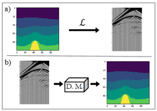
Figure 1: Diagram illustrating (a) forward modeling and (b) inversion processes in seismic velocity studies utilizing deep learning-based models. The seismic propagation equation, $\mathcal{L}$, facilitates the computation of seismic data; however, no explicit equation is available for deriving velocity based on existing seismic data.

$$D=\mathcal{L}(m_{v})$$ (1)

In (1), $D$ is seismic data, and $m_{v}$ is velocity model parameters. In this study the $\mathcal{L}$ is 2D acoustic wave equation (see Eq. 7). It can be solved by different numerical methods but there is no equation or straight way to reverse the direction of $\mathcal{L}$ in Fig. 1(a). Mathematically the inverse of $\mathcal{L}$ gives $m_{v}$ as shown in Eq. (2).

$$m_{v}=\mathcal{L}^{-1}(D)$$ (2)

The inverse operator (represented as $\mathcal{L}^{-1}$) is crucial for predicting the velocity model parameters that best fit the empirical seismic data. This process represents a complex nonlinear inversion problem, where adjustments to the velocity parameters do not manifest in a directly proportional response within the seismic data observations. Furthermore, the issue is inherently ill-posed, as it permits the existence of several sets of velocity parameters that can produce equivalent seismic data, thereby complicating the solution’s uniqueness and stability.

Addressing this nonlinear ill-posed problem, researchers have explored a diverse range of methodologies. These span from global methods, which utilize Eq.(1) to identify an optimal $m_{v}$ by investigation in velocity model domain [27], to derivative-based approaches. The latter initiate with an initial model $\bar{m}_{v}$, subsequently compute the corresponding seismic data $\bar{D}$, and adjust the $\bar{m}_{v}$ parameters to minimize the local gradient of $L(D-\bar{D})$ [28], [5] (L is the loss function). More recent advancements have seen the emergence of deep learning-based techniques, providing innovative solutions to this long-standing problem [24], [11], [25], [12], [13].

The deep learning model can be mathematically represented as shown in Eq. (3):

$$\mathcal{F}(D^{n},\mathcal{W})\rightarrow m^{n}_{v}$$ (3)

Here, $\mathcal{F}$ denotes the deep learning function responsible for transforming the seismic data, $D^{n}$, into a velocity model, $m^{n}_{v}$. $\mathcal{W}$ represents the set of learnable parameters or weights within the model. If N is the total number of training dataset, then each individual training sample can be denoted by n, such that n $\in$ N. The function $\mathcal{F}$ is composed of multiple neural network layers, each with varying depth and connection patterns, extending from the input to the output layer. The input data propagates through these layers to produce an output. This output is then compared to the ground truth or target and the distinction between them is quantified through the utilization of the loss function. The success rate of the deep model is influenced by both the quantity and comprehensiveness of the training dataset.

In this study, seismic sources were evenly distributed above the velocity models and scanned at various angles to produce seismic shot gathers. A total of 20 shot points were utilized, resulting in 20 distinct seismic shot gathers. These shot gathers are presented to the deep neural networks as input, with the corresponding velocity model serving as the ground truth.

In our research, we employed Convolutional Neural Networks (CNNs) based deep model to establish a clear link between the seismic data’s characteristics, such as direct arrivals, reflections, scattering, and potential refractions, and the underlying velocity model parameters (Fig. 1(b)) such as inter-layer velocity value, number of layers, layers interface shape, salt dome, and fault properties. To achieve this, we designed a neural network with a layered structure that is deep enough to maintain the integrity of the gradient flow during training. We introduced an encoder-decoder framework in our neural network, which allows us to train on complex models directly, bypassing the need for initial data manipulation or pre-processing. Furthermore, by integrating a Dense network structure, we were able to construct more robust neural network layers while ensuring that the gradient signal does not weaken significantly as it travels through the network. The details of this neural network design are elaborated in Section III-B.

III-A Dataset Preparation

To establish the training and test datasets, we first generated velocity models, followed by seismic shot gathers. In all, we prepared 18,000 velocity models. These models are categorized into five groups, with the number of layers ranging from 4 to 8. Each group is further divided into three subgroups: stratified, faulty, and salt dome, with each subgroup containing 1,200 models. For every velocity model, we calculated 20 shot gathers. Each seismic data has a time dimension of 1 second and encompasses 34 receivers. All computations are carried out in a constant density acoustic environment, with velocity values increasing in correlation with depth.

III-A1 Velocity Models

In order to prepare realistic velocity models, we closely examined published stratigraphic examples and incorporated geological principles into our approach. Consequently, inclined, undulating interfaces, normal and reverse faults with varying angles and fault throw, and salt bodies with arbitrary size, shape and horizontal positions are used.

To prepare interfaces resembling subsurface stratigraphic formations, we generated 116 distinct interface curves using various mathematical functions, including trigonometric, polynomial, and logarithmic. Eq. (4) through (6) display three examples of these functions.

$$l_{1}=\sqrt{x}+5\log(15x+1)\sin(0.14x)\cos(0.3x+20)$$ (4)

$$l_{2}=0.09x^{2}-3.6\sin(0.6x+2)+5(x+1.5)-0.8x$$ (5)

$$l_{3}=e^{(0.1x-0.11)}-1.5\sin(x-6)+2.1\frac{x}{x+3}$$ (6)

The interfaces are saved as integer values. The velocity model is created by randomly selecting the depth, interface shape, and velocity value for each layer, with the process commencing from the top layer and continuing downwards. This process for each velocity layer is illustrated in Alg. 1.

Two principles are considered in this process. First, the velocity value increases with depth, meaning that the lower layer always has a higher velocity than the upper one. Second, to partially maintain the geological sediment deposition logic between the layers, the shape of the interfaces above is influenced by those below. Consequently, the stochastically chosen interfaces merge with the ones below. The inter layer velocity value varies between [1500, 4000] m/s.

Algorithm 1 Layer Filling Algorithm

0:  Stochastic selection of parameters

  Initialize $d_{prev}\leftarrow 0$

  Initialize $L_{prev}\leftarrow 0$

  $V_{i}\leftarrow$ Choose velocity value for the layer

  $d_{i}\leftarrow$ Choose depth of the layer

  $L_{i}\leftarrow$ Choose interface of the layer

  $spaceStart\leftarrow d_{prev}+L_{prev}$

  $spaceEnd\leftarrow d_{prev}+L_{prev}+d_{i}+L_{i}$

  Fill the space between $spaceStart$ and $spaceEnd$ with $V_{i}$

  Update $d_{prev}\leftarrow d_{prev}+d_{i}$

  Update $L_{prev}\leftarrow L_{prev}+L_{i}$

The minimum velocity difference between layers is 200 m/s. In a medium characterized by constant density, the velocity contrast across layer boundaries plays a crucial role in determining the reflection coefficient. Particularly, within layers with higher velocity values, a small contrast results in a significant decrease in the amplitude of the reflected wave. The size of the velocity models is 100$\times$100 grid points.

We created fault models by incorporating fault line code into the prepared layered models algorithms. The angle of line, fault type (normal and reverse), and fault throw value is chosen stochastically. According to the type of fault the hanging wall part of the model moved up or downward across the fault line.

To construct the models with a salt dome at least four different Gaussian functions are generated stochastically and their combinations are utilized. This approach enables the creation of salt domes with diverse sizes and shapes. The dome’s velocity values change between [4350, 4550] m/s. The intrusion of a salt dome into the overlying sediments deform the shape of the upper layers. For inducing this deformation in the upper layers of the salt domes, we employed wider Gaussian functions. Some sample velocity models are depicted in Fig. 2.

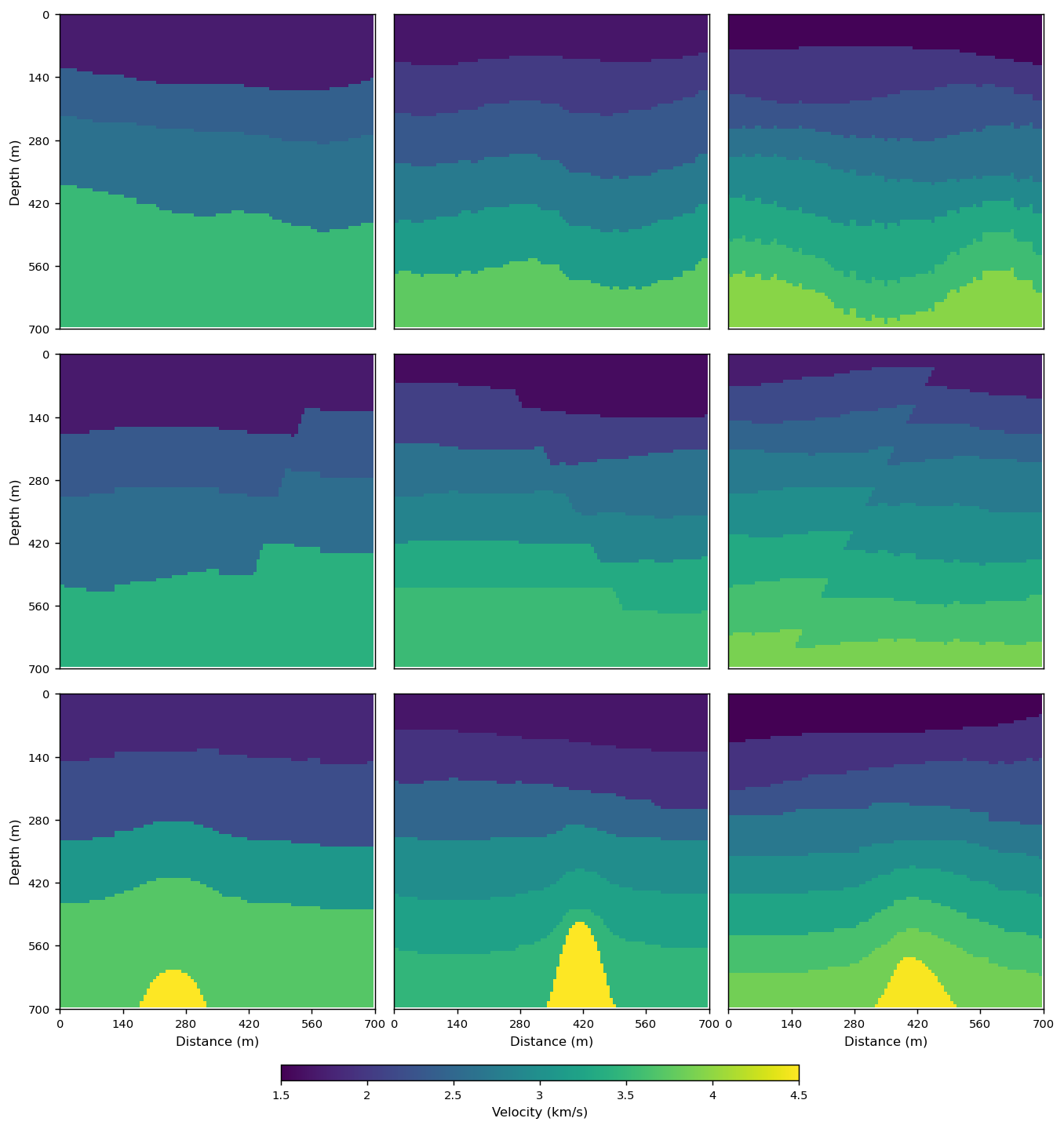
Figure 2: Samples from our dataset; top: layered, middle: fault, bottom: salt dome velocity model samples. The samples are selected from 4, 6, and 8 layered models. The model’s spatial resolution is $700\times 700$ m.

III-A2 Seismic Data

In order to calculate the seismic shot gathers presented to the deep model as input, 34 receivers and 20 sources are distributed uniformly along the upper boundary of the velocity models. To capture data from the lateral portion of the velocity models, we positioned the receiver at both the initial and final grid points. Given a receiver interval of 3 grids with an evenly distributed setup, the total number of receivers is determined to be 34. The source locations are initiated from the third grid point and proceeded with intervals of 5 grids, reaching the 98th grid. The time progression of the seismic wavefield in a 2D acoustic environment is calculated by Eq. (7).

$$\frac{\partial^{P}}{\partial t^{2}}-v^{2}(\frac{\partial^{2}P}{\partial x^{2}}+\frac{\partial^{2}P}{\partial z^{2}})=\mathcal{S}(t,x,z)$$ (7)

Where P is the acoustic wavefield, $v$ is the seismic velocity of the medium, $x$ and $z$ are spatial coordinates, $\mathcal{S}$ is the source function and $t$ is time. The numerical solution of Eq. (7) is implemented in the time domain by 2D finite difference method [29]. Seismic data is computed for a duration of 1 second at each individual receiver location. The Ricker wavelet with a dominant frequency of 20 Hz is used as the seismic source. To mitigate dispersion in the numerical computation, the spatial environment is sampled at intervals of 7 meters, adhering to the Alford et al. [30] condition and considering $v_{min}=1500$ m/s alongside the source frequency (20 Hz), in other words $\Delta x=7$m. To simplify the calculation $\Delta z=\Delta x$. Considering the $\Delta x$ value and $v_{max}=4550$ m/s, to ensure the accuracy of numerical computations, we set the time sampling intervals to 1ms (Lines et al.[31] condition), in total 1000 time samples. In order to minimize the effect of boundaries, 20 grid points are added on the right, left and bottom of each velocity model and Clayton and Engquist [32] absorbing boundary conditions are used. Consequently, seismic data of dimensions [20, 1000, 34] are acquired for each velocity model. Fig. 3 illustrates 1th, 10th, and 20th shot gathers corresponding to the randomly chosen velocity model.

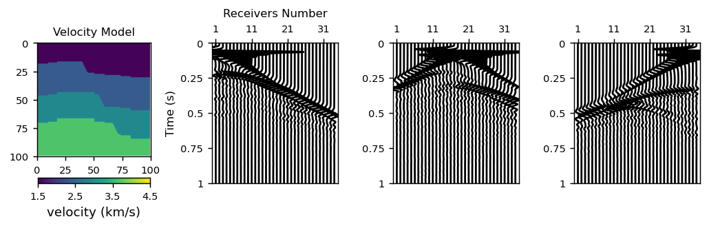
Figure 3: The velocity model and its associated synthetic shot gathers at the first (a), tenth (b), and twentieth (c) source locations.

To partially reduce the disparity between the synthetic and real seismic data, both coherent and random noise are added to the prepared dataset. Coherent noise is derived from the characteristics of surface waves. Hence, spike patterns, characterized by velocity values ranging from 250 to 450 m/s, are generated in such a way that the maximum amplitude is observed at the proximal receiver. These patterns exhibited a progressive attenuation with temporal advancement. Subsequently, a Ricker wavelet with a central frequency randomly chosen between 8-17 Hz as the source of the surface waves is convolved with the spikes gather. Through the application of this stochastic algorithm to each velocity model, 18,000 coherent noise gathers are produced, demonstrating the impact of surface waves.

To generate random noises, initially, white noise with a randomly selected standard distribution, and zero mean is created. In the subsequent phase, certain randomly chosen segments of the produced noise are assigned a value of zero, and it is convolved with a sine function characterized by a randomly selected frequency value falling within the range of 13 to 17 Hz. The computed noisy data is then added to the seismic shot gathers, resulting in the acquisition of a noisy dataset. One sample of the stochastic, coherent, noiseless and noisy shot gather is shown in Fig. 4.

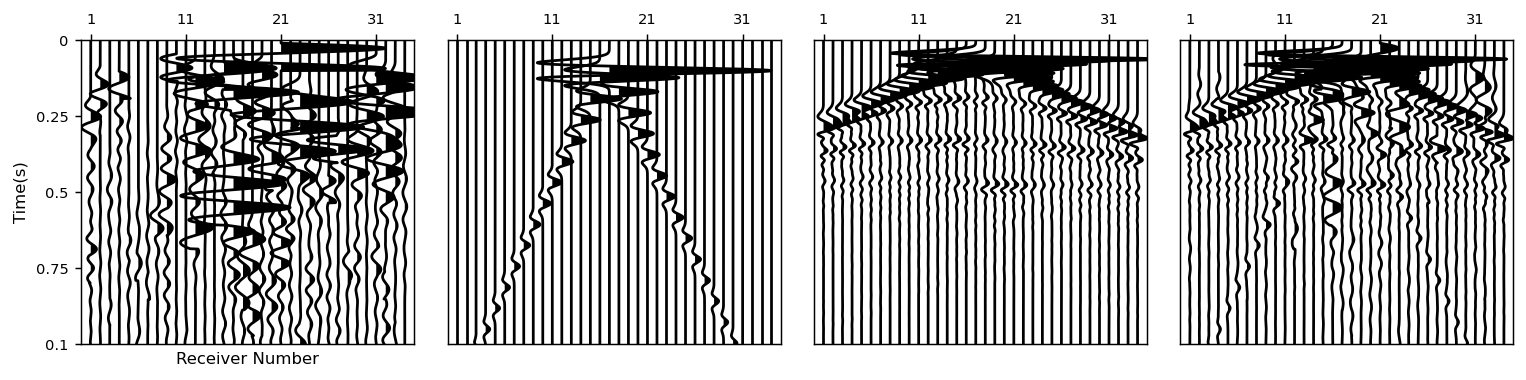
Figure 4: The samples of stochastic, coherent, noiseless and noisy gather are arranged from left to right, respectively. The gathers are plotted on the same scale.

III-B Architecture of the Deep Model

In this study, we take the design of the InversionNet [11] deep model as the baseline. Similar to InversionNet, we employ one-dimensional (1D) CNN kernels to reduce the time axis of the input data to the number of receivers within the initial four layers. However, unlike InversionNet, we do not reduce the size of the features below 6$\times$6. This decision is based on the understanding that the amplitude of adjacent traces contains crucial information pertaining to the structure of the velocity model interfaces.

In our deep model architecture (Fig. 6), both the encoder part and the decoder part consist of different dense blocks (depicted as blue blocks in the figure) with fixed feature size and transition layers in order to speed up the information flow and prevent the fading of the gradients during backpropagation. Furthermore, certain outputs from the dense blocks in the encoder segment are concatenated with features of the same size in the decoder part. To avoid excessive layer addition, the experimentation commenced with a shallow CNN model. Based on the findings, subsequent improvements are implemented by incorporating new layers and dense blocks into the model structure. Owing to the structured design of the dense blocks in our architecture, we can expand the number of layers and concatenate their output features without the need for a progressive increase in channel size.

III-B1 Dense Block Structure

Within each dense block, there are 3 CNN layers, with the feature size matching that of the initial layer. Fig. 5 illustrates the schematic representation of the i-th dense block, and the connections between its layers. Equations (8)-(12) describe i-th dense block mathematically.

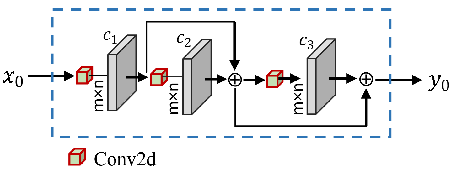
Figure 5: A dense block with 3 layers.

$$x^{i}_{1}=L^{i}_{1}(x_{0})\hskip 5.78172pt;\hskip 5.78172ptC_{out}=c_{1}$$ (8)

$$x^{i}_{2}=L^{i}_{2}(x_{1})\hskip 5.78172pt;\hskip 5.78172ptC_{out}=c_{2}$$ (9)

$$x^{i}_{1,2}=concatenate(x^{i}_{1},x^{i}_{2})$$ (10)

$$x^{i}_{3}=L^{i}_{3}(x^{i}_{1,2})\hskip 5.78172pt;\hskip 5.78172ptC_{out}=c_{3}$$ (11)

$$y_{0}=concatenate(x^{i}_{1},x^{i}_{2},x^{i}_{3})$$ (12)

Here, $L^{i}_{j}$ is the j-th layer of a dense block i, $x_{0}$ is input to the dense block and $y_{0}$ is the output of i-th dense block; $x^{i}_{j}$ is the output of the j-th layer. $c_{j}$ shows the channel size (i.e. number of feature maps generated), which determines the depth of the output volume, in each layer. In our architecture $c_{j}$= 64 and $y_{0}$ has 192 feature maps, and $L_{j}$ contain a 3$\times$3 convolution (Conv), batch normalization (BN) [33] layers, and rectified linear unit (ReLU)[34] activation function. For the sake of convenience, this combination, conv2d+BN+ReLU, will be referred to as the Con2D in our discussion from this on. In the transition layers between the dense blocks with identical feature sizes the channel size of the output is typically reduced (as shown with purple cubes in Fig. 6).

III-B2 Encoder Network

Through the utilization of 1D-CNNs for the initial four layers (depicted with orange arrows in Fig.6), the time dimension of the input data is reduced based on the number of receivers. In other words, the output dimension of the fourth layer is 34$\times$34. Subsequently, the data dimensions are progressively reduced to 18$\times$18, 9$\times$9, and 6$\times$6 through the application of 2D-CNNs. For the 34$\times$34 dimension, there are three dense blocks, whereas for the other dimensions, there exist 2, 1, and 1 dense blocks, respectively. There are three Conv2d layers within each dense block. Each layer’s input comprises the outputs of the preceding layers. Therefore, the CNN kernels are able to utilize the features extracted in the preceding layers to access low level features.

The outputs of the dense blocks with identical feature sizes are concatenated and subsequently fed into the Conv2d layer where their size can be reduced via stride values exceeding one. As a result, the size of output channels decreases during the transition from these layers and the output from these layers is used as the input to a new dense block. In Fig. 6, these layers are depicted using small red-green cubes.

III-B3 Decoder Network

The features extracted within the layers of the encoder model are progressively scaled to dimensions of 9$\times$9, 18$\times$18, 34$\times$34, 51$\times$51, and 100$\times$100 in order to construct the output corresponding to the velocity model. For sizes 34$\times$34 and 51$\times$51, two dense blocks are utilized for each, whereas a single dense block is employed for size 100$\times$100. The process of scaling up takes place within the layers, which comprise upsampling and Conv2D operations. (The small blue-yellow cubes in Fig.6 depict these layers.) In order to facilitate the information transfer process and consolidate the decoder part features, the outputs of the dense blocks with a size of 18$\times$18 and 34$\times$34 in the encoder part are also concatenated with their corresponding counterparts in the decoder part. Due to the incorporation of dense blocks, this architecture enables an increase in the channel size, allowing for the processing of larger feature sizes without a rise in the number of parameters. The inclusion of a 100$\times$100 dimensional dense block before the output layer proves to be instrumental in the efficacy of the deep model. The output of this dense block undergoes a Conv$1\times 1$ + Sigmoid activation function, yielding the deep model output (depicted with a green arrow in Fig.6).

In this proposed architecture, on the one hand, features are extracted from seismic data and aligned with the size and dimensions of the velocity model, while on the other hand, the essential information required for this alignment can be easily transferred between the input and ground truth. The number of parameters of SVInvNet is about 4 million.

The output of this architecture is compared with the ground truth, and the disparity between them is computed using the loss function. The loss function should be capable of capturing the disparity among the velocity values as well as the shapes of the interfaces and geological structures between two velocity models. Hence, in this section of the architecture, we employ both mean absolute error (L1) and structural similarity index measure (SSIM) as loss functions, and we assign weights to each of them using two coefficients ($\lambda_{L1}$ and $\lambda_{SSIM}$ ) to enhance the derivatives of the loss functions.

IV Experiment and Results

We generate 18,000 data samples in total, with 3,600 models for each group. For instance, in a model with seven layers there are 3 different subgroups: dense layered, faulty and salt dome; 1,200 models for each subgroup.

Since the layer count in the dataset range from 4 to 8, the total number of models can be computed as 5$\times$3$\times$1200. From each of the 15 different types of data, 800 models are randomly selected as part of the test benchmark. Hence, the total number of test dataset size is 12,000. The remaining models in the dataset (i.e. 6,000 models) are used as the training dataset. To investigate the impacts of varying the quantity of training data on the mapping or seismic inversion process, we prepared five different training datasets. Accordingly, we selected various quantities of subgroups, as 50, 100, 200, 300, and 400 models from each subgroup. Consequently, we undertook five separate training processes with 750 (15$\times$50), 1,500, 3,000, 4,500, and 6,000 training dataset sizes and evaluated the trained deep models using the same test benchmark that we prepared using 12,000 models. For the purposes of clarity and convenience, we introduce a nomenclature to denote the various training datasets. Specifically, we assign Roman numerals I-V to represent training datasets corresponding to sample sizes of 750, 1500, 3000, 4500, and 6000, respectively. Hence, these datasets will be referred to as TD-I, TD-II, TD-III, TD-IV, and TD-V, respectively.

The number of test data is at least twice that of the training datasets, enabling an investigation into the generalization ability of the trained deep model. For example, TD-IV contains 300 models of each velocity subgroups, in terms of number of samples, it corresponds to 37.5% of the test benchmark size. The training conditions remained identical across all five training processes. Employing a consistent nomenclature for the trained models, we extend the use of Roman numerals I-V to the designation of our train models. For instance Model-I will be corresponding to the model that is trained with TD-I and so on.

TABLE I: Training Hyperparameters

Hyperparameter	Value
Optimizer	Adam
Initial learning rate	5.0 e-3
Epoch	500
Batch size	32

For every velocity model, 20 shot gathers with 34 receivers are computed for a 1-second duration with a 1ms temporal sampling interval. The source interval is 35 m and the receiver interval is 21 m. Consequently, the size of the input data is [20, 1000, 34], while the size of the ground truth data (velocity model) is [1, 100, 100]. We established the network hyperparameters based on the results of various experiments. For optimization, the Adam optimizer [35] is utilized with a batch size of 32, and the initial learning rate is set to 5e-3. During the training, the learning rate is adjusted by gradually decreasing it in accordance with the optimization process. The number of epochs for all training processes is set to 500. The training hyper parameters of the deep model are depicted in Table I.

To compute the misfit and similarity between deep model predictions and the ground truths in the test stage, we utilize mean absolute error (L1) and mean square error (L2), structural similarity index measure (SSIM), and multi-structural similarity index measure (MSSIM). A successful estimation of velocity model or velocity inversion is characterized by lower L1 and L2 values, as well as higher SSIM and MSSIM values. These values are computed for the normalized dataset. All training and testing procedures are executed on GPUs, on an NVIDIA RTX A4500 graphics card, using PyTorch library.

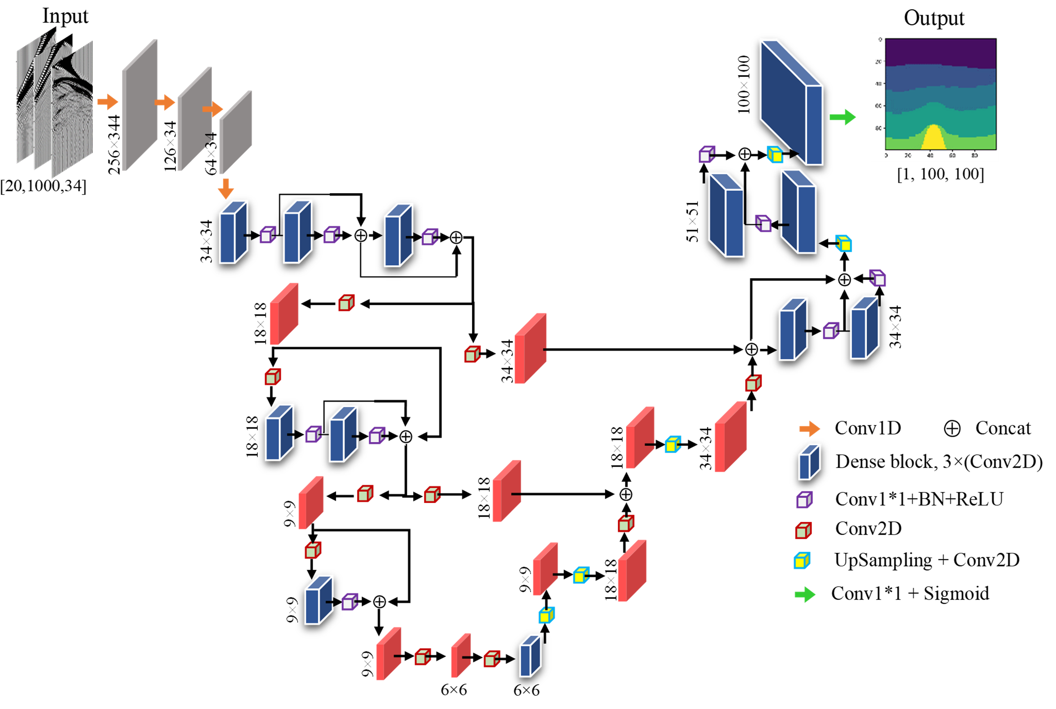
Figure 6: Proposed SVInvNet architecture for seismic velocity inversion.

TABLE II: The Performances of the Three Versions of InversionNet on the Test Dataset, trained using Noiseless TD-V.

	InversionNet($\alpha$)		InversionNet($\beta$)		InversionNet($\gamma$)
Metric	L1	L1 + SSIM	L1	L1 + SSIM	L1	L1 + SSIM
L1	0.008797	0.008828	0.008574	0.008385	0.007249	0.007316
L2	0.000497	0.000499	0.000485	0.000471	0.000407	0.000401
SSIM	0.999970	0.999970	0.999972	0.999973	0.999977	0.999978
MSSIM	0.999997	0.999997	0.999997	0.999997	0.999997	0.999997

IV-A Baseline Model

To compare the performance of SVInvNet, we employed the InversionNet model, proposed by Wu et al. [11], as the baseline. Li et al.[12] also used the InversionNet as the baseline, with certain modifications made to its architecture. Despite slight disparity, the architecture introduced by Li et al. [12] yields better results than Wu et al. version in our experiments. The parameter count for both versions of InversionNet is around 44 million.

We also made certain modifications to the InversionNet, resulting in a new version that outperforms the previous iterations (Table II). For convenience, we use $\alpha$, $\beta$, and $\gamma$ to denote Wu et al. [11], Li et al. [12], and our variant of InversionNet models, respectively. The tabulated data in Table III shows the parameter counts for each of the three iterations of both the baseline and SVInvNet.

As for the modifications, we replaced the MaxPooling function with a Convolution function in the fourth layer of the InversionNet($\alpha$) and decreased the feature size until it reached 4$\times$4 instead of 1$\times$1. Furthermore, by substituting each deconvolution layer with an upsample + convolution approach in the decoder segment of the model, the parameter count decreased to 20 million, leading to an enhancement in the prediction capabilities of the new version.

TABLE III: Model Sizes

Deep Model	Parameter Count(M)
InversionNet($\alpha$)	44
InversionNet($\beta$)	44
InversionNet($\gamma$)	20
SVInvNet	4

IV-B Results and Discussion

The three variants of InversionNet are trained with the TD-V separately and tested with our test benchmark. In order to examine the implications of the loss function, the training stage is conducted twice, once incorporating the L1 loss function and once integrating both the L1 and (1-SSIM) loss function depicted as L1+SSIM. The statistics of misfit and similarity metrics in the test stage are presented in the Table II.

As per the findings depicted in Table II, InversionNet($\gamma$) demonstrates superior capability in acquiring the mapping of seismic data to the velocity model in quantitative comparison to versions $\alpha$ and $\beta$. Additionally, the L1+SSIM loss function effectively captures disparity between the output of the deep model and the ground truth, surpassing the performance of the sole L1 loss function in this aspect.

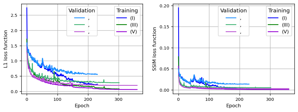
Figure 7: The L1 (Left) and SSIM (Right) loss curves on the training and validation datasets obtained during the training of Model-I-III-V.

Additional experiments are carried out on the noisy dataset utilizing the L1+SSIM loss function. In this context, we utilized the noisy TD-V to train three versions of the InversionNet separately. Subsequently, we employed the noisy test benchmark to establish the testing process. The performances of the models using four metrics for the noisy test set are presented in Table IV. As can be seen, our improved version of InversionNet demonstrates better performance over InversionNet($\alpha$) and similar performance to InversionNet($\beta$). Consequently, we utilized the InversionNet($\gamma$) as the baseline for our benchmark model evaluations for the upcoming experiments.

TABLE IV: The Performances of the Three Versions of InversionNet on the Test Dataset, trained using Noisy TD-V.

InversionNet	($\alpha$)	($\beta$)	($\gamma$)
L1	0.014378	0.013028	0.013142
L2	0.000765	0.000706	0.000713
SSIM	0.999943	0.999950	0.999949
MSSIM	0.999994	0.999995	0.999995

Utilizing the noiseless and noisy versions of our TD-I to TD-V, we independently trained SVInvNet and subsequently evaluated each of the resultant five trained deep models (Model-I to Model-V) using our test benchmark, which is identical for all models with 12,000 data pairs. The misfit and similarity values of the test phases for the noiseless dataset are shown in the Table V. As anticipated, increasing the volume of the trained dataset corresponded to a decrease in the values of L1 and L2, alongside an increase in the values of SSIM and MSSIM. The L1 and SSIM loss function curves on the training and validation datasets during the training are depicted for three selected models aggregated in Fig. 7. From the plots, it is evident that Model-I exhibits overfitting behavior. However, as the training dataset size increases (refer to Model-V), this issue is significantly reduced.

Increasing the number of samples in the training dataset resulted in a decrease in loss function values, an improvement in similarity measures, and an extension of the training phase duration. Based on the results presented in Tables II and V, it is evident that the performance of our proposed deep model surpasses that of the InversionNet. Even the loss values of SVInvNet, trained with TD-III, indicate a superior performance compared to the values of the InversionNet($\gamma$), trained with TD-V. In other words, our deep model can map seismic shot gathers to velocity models better with lower loss function than the baseline model.

Qualitative evaluations of our trained models are depicted for randomly selected test samples in Fig. 8. Each sample is purposefully selected from 8-layer group to showcase the visuals from more challenging group with respect to the inversion for layered, fault, and salt dome categories. The ground truth and the predicted result of Model-I, Model-III, and Model-V of these samples are depicted in Fig. 8. For qualitative assessments, we pay attention to the velocity value and the interface shape of the layers, the fault line continuity, and throw value as well as the shape, position, and velocity value of the salt dome. As can be seen from the samples, the velocity values within the layers remain constant. With an increase in the size of the training dataset, the discrepancies in the approximation of this value diminish, gradually converging towards a stable and unvarying value. Evident from the velocity profile depicted in the same figure on the right column, the blue line, associated to Model-I, exhibits more pronounced oscillations compared to the green line (corresponding to Model-III), while the green line displays greater oscillatory behavior than the red line (Model-V). Notably, minimal oscillation is observable in the red line.

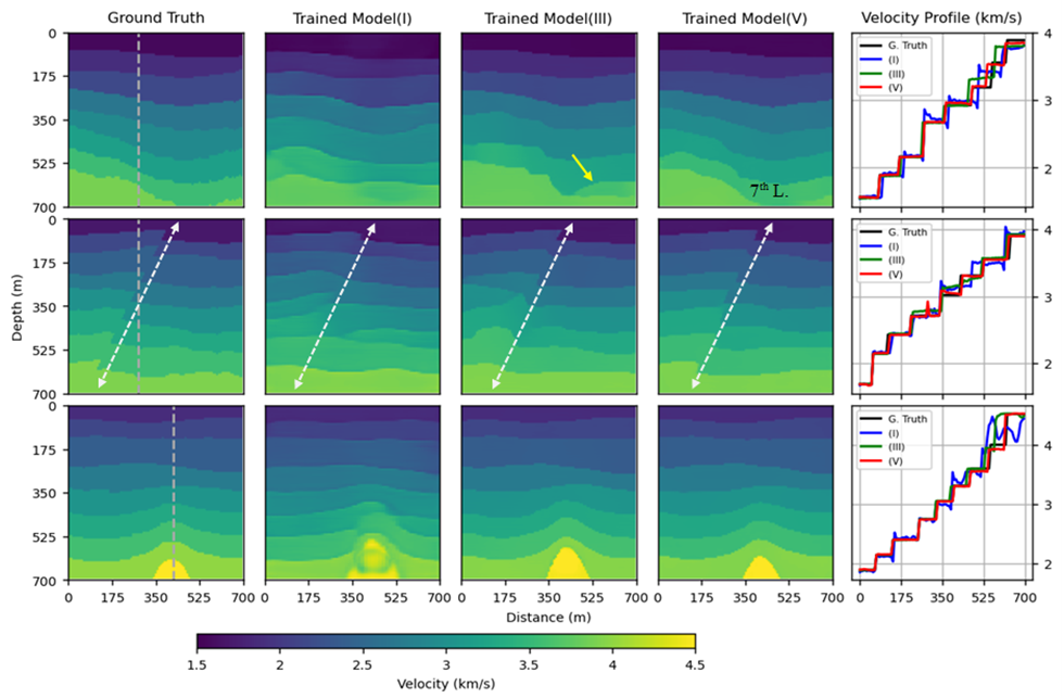
Figure 8: Ground truth velocity model and the prediction results of our Model-I (the second column), Model-III (the third column), and Model-V (the fourth column). The rightmost column shows a vertical velocity profile at the gray line depicted in the ground truth model for four velocity models.

TABLE V: The Performance of Our Deep Models on the Test Set. Models I-V are trained using Noiseless TD I-V, respectively.

	Model-I	Model-II	Model-III	Model-IV	Model-V
L1	0.013680	0.009833	0.006844	0.005301	0.004944
L2	0.000737	0.000509	0.000356	0.000272	0.000253
SSIM	0.9999436	0.9999674	0.9999810	0.9999870	0.9999884
MSSIM	0.99999491	0.99999692	0.99999812	0.99999870	0.99999882

As the depth increases, predicting the shape of the layer interfaces and velocity values becomes increasingly challenging. From a geophysical standpoint, as the seismic wave propagates through various subsurface layers, a portion of its amplitude and thus its energy is lost due to reflection back to the Earth’s surface. The decrease of energy gives rise to reduction in the amplitude of seismic data reflected from deeper interfaces, particularly in cases characterized by a lower reflection coefficient. Thereby, as the number of layers increases, seismic data originating from deep interfaces exhibit decreased amplitudes and insufficient information. Hence, the amplitude of the data recorded by receivers diminishes over time, posing a challenge for CNN kernels in the extraction of features from seismic data. In Fig. 8, in the first-row, Model-I encountered challenges in constructing the 7th layer of the velocity model and resorted to distributing this layer between the 6th and 8th layers. Conversely, Model-III modified the shapes of the 6th and 8th layers, and constructed a portion of the 7th layer, as indicated by the yellow arrow. Model-V, in contrast, could successfully constructed the 7th layer.

In fault models, the presence of abrupt angles along the fault lines perturbs the trajectory of the reflective hyperbola. Concurrently, diffractions arising at proximal surface interfaces result in the attenuation of reflections and diffractions from deeper strata, a phenomenon that becomes particularly evident when the displacement of the fault, or fault throw, is relatively short.

This complexity is amplified particularly in the case of faults located in close proximity to the edges. As the quantity of training dataset samples increased, the deep model demonstrated an enhanced ability to successfully construct the shapes of fault lines and faulty interfaces. The white arrows delineate the actual position of the fault line in the velocity models, facilitating ease of comparison.

The salt dome has distinctive properties in both velocity value and shape, different from the surrounding layers. Seismic waves encountering the apex of a salt dome undergo scattering, thereby creating a noticeable scattering pattern. However, due to its placement in the lower layer, the amplitude of these scatterings is considerably smaller when compared to the reflection data. As observed in the third row of Fig. 8, the deep model trained with a lower number of training data identified the scatterings originating from the layers above the salt dome as belonging to a large salt body; with an increased number of training samples, the other two models exhibits an improved capability to discern the structural characteristics of the salt dome and differentiate the scattering caused by it from the surrounding layers.

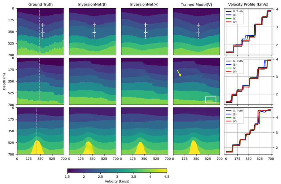
Figure 9: Ground truth velocity model and prediction results of InversionNet $\beta$ and $\gamma$ version and our Model-V. The rightmost column shows a vertical velocity profile at the gray line depicted in the ground truth model for four velocity models. The white dashed lines in the models of the first row are employed to illustrate the local position of the second and third interfaces. The yellow arrow and white rectangular within the faulty velocity model of Model-V are employed to highlight the alteration of the third interface and the estimation of impact of the fault on the sixth interface, respectively.

TABLE VI: The Performance of Our Deep Models on the Test Set. Models I-V are trained using Noisy TD I-V, respectively.

	Model-I	Model-II	Model-III	Model-IV	Model-V
L1	0.024961	0.018942	0.014189	0.010378	0.008034
L2	0.001548	0.001044	0.000736	0.000489	0.000399
SSIM	0.999856	0.999911	0.999945	0.999967	0.999977
MSSIM	0.999988	0.999992	0.999995	0.999997	0.999997

For visual comparison of the performance between InversionNet $\beta$ and $\gamma$ version and our Model-V, three samples selected randomly from seven layered models are illustrated in Fig. 9. The deep models are trained with noiseless TD-V. In the layered velocity model depicted in the first row of Fig. 9, the second and third interfaces display curvature, and the velocity contrast between the third and fourth layers is relatively minimal. As a result, the amplitude and trajectory of the reflected hyperbolas from the second and third interfaces are weakened and demonstrate greater complexity compared to the other interfaces. The white dashed line delineates the locations of the second and third interfaces at a specific point. The results from our developed model surpass those of InversionNet($\gamma$), and InversionNet($\gamma$)’s results, in turn, outperform those of InversionNet($\beta$). This superior performance is also maintained in samples featuring fault or salt dome.

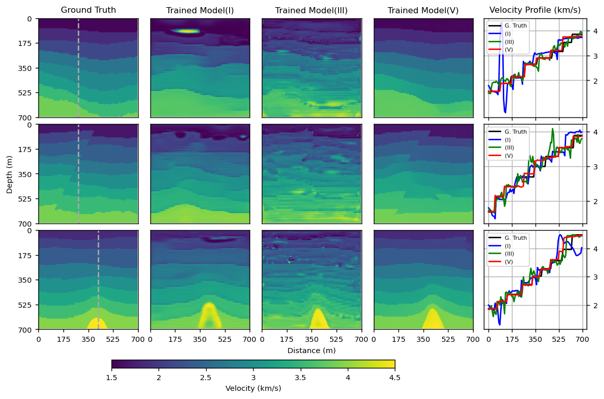
Figure 10: Prediction outcomes of our models for the noisy dataset. The first column corresponds to the ground truth (target) velocity model, while the rightmost column displays a vertical velocity profile along the gray line depicted in the target model for four velocity models. The velocity models are the same as Fig. 8.

The introduction of noise to the data exacerbates this situation, causing distortion in the amplitude of the signal emanating from the interfaces and deforming the trajectory of the scattering or reflection hyperbola. This further complicates the process of extracting features from the seismic gathers performed by CNN kernels. The adverse impact of noise in the velocity mapping process is evident based on the performances presented in Tables VI and V. Upon examining the results in Table IV and VI, it is evident that SVInvNet demonstrates superior performance, even in the presence of noise, when compared to the InversionNet different versions.

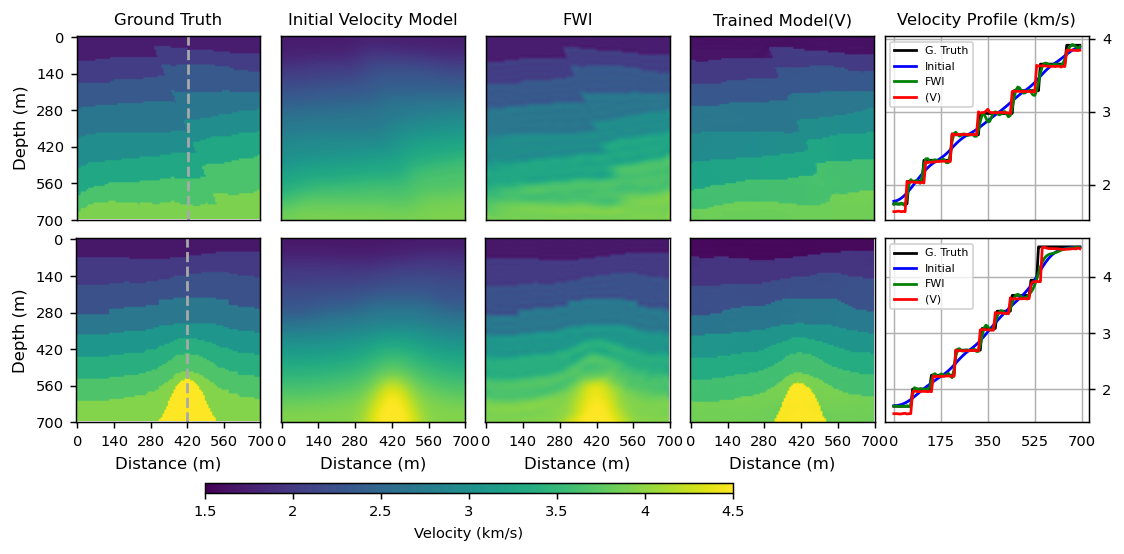
Figure 11: Comparison of FWI and Model-V results. The columns corresponds to the ground truth, initial, FWI result, and Model-V estimation velocity model respectively, while the rightmost column displays a vertical velocity profile along the gray line depicted in the ground truth model for four velocity models.

Fig. 10, depicts the predicted velocity values of SVInvNet trained with noisy TD-I, TD-III, and TD-V. The performances of Model-I and Model-III show significantly inferior results compared to the corresponding noiseless cases. The prediction results presented in Table VI substantiate this, especially when compared with similar items in Table V. To successfully construct the velocity model by capturing the signal within noisy data and discerning its pattern, the deep model requires a greater number of samples for supervision. In other words, an increased sample size is imperative for the model to effectively filter out noise and accurately learn the desired signal.

IV-B1 Comparison with FWI Method

In this section, a comparison was conducted between the outcomes of the Model-V and the derivative-based FWI method using examples of velocity models featuring fault and salt dome. Fig. 11 illustrates that the velocity models derived by Model-V exhibit a closer alignment with the ground truth when contrasted with the FWI method.

Due to the high sensitivity of the FWI method to noise, noise-free datasets are used. Initial velocity model is acquired through Gaussian smoothing with a standard deviation of $5$ applied to the ground truth model. To minimize the cyclic skipping effect [9], we executed the process with the selection of five cutoff frequencies within [10, 15, 20, 25, 30] Hz. Furthermore, a condition was introduced by limiting the velocity parameters between 1000 and 5000 m/s to enhance the efficacy of the FWI method. The entire process is performed for a total of 50 iterations. The computational configuration employed for seismic shot gathers in the trained data segment remains consistent with the setup utilized in the FWI procedure. To implement FWI, the DeepWave[36] package is employed.

As illustrated in Fig. 11, FWI encounters challenges in estimating the shape of deeper layer interfaces, despite having a strong initial model. Furthermore, the velocity models between layers in the FWI estimation exhibit non-constant behavior and display oscillatory patterns. The profile section, green line representing FWI results, reveals heightened instability compared to the red line representing Model-V result.

Concerning the salt dome, while the initial velocity model provides a somewhat clear indication of the salt dome’s location and distribution, Model-V demonstrates superior performance in inverting both the shape and velocity values of the salt mass in compare with FWI method.

V Conclusion

In this study, we introduce a novel end-to-end deep model, SVInvNet, for seismic velocity inversion. In order to enhance the capacity of SVInvNet in learning and estimating more complex velocity models, we abstained from merely increasing the channel number of CNN layers (i.e. number of feature planes), which cause an excessive increase in the number of parameters. Instead, we devised a network architecture characterized by the multiple connections among its layers with only 4M parameters. This design facilitated the efficient flow of information between the input and the corresponding ground truth. Based on the outcomes derived from both noisy and noiseless datasets, SVInvNet demonstrates proficiency in accurately estimating velocity models characterized by multilayer structures, fault, and salt dome. Furthermore, it is observed that increasing the quantity of training dataset correlates with a reduction in loss function in the testing phase. The utilization of a test dataset size at least twice that of the training datasets reveals the comprehensiveness of the results produced by the trained SVInvNet.

The results obtained from the dataset containing both random and coherent noise emphasize the capability of SVInvNet to effectively filter such noise types and map seismic data to velocity models. However, attaining an equivalent loss function value as observed in the noise-free dataset necessitates a larger training dataset in the presence of noise.

Mojtaba Najafi Khatounabad received the bachelor’s degree in Nuclear Physics and the master’s degree in Geophysics from Urmia University, Urmia, Iran, in 2010, and 2014 respectively. In 2017, he was awarded a full Ph.D. scholarship by Türkiye Scholarships. He is currently pursuing the Ph.D. degree in Engineering Geophysics with Institute of Science and Technology, Ankara University, Ankara, Türkiye, under the supervision of Prof. Dr. Selma Kadioglu and Assoc. Prof. Dr. Hacer Yalim Keles. His research interest includes seismic modeling, full-waveform inversion, and deep-learning-based geophysical data processing and inversion.

Dr. Hacer Yalim Keles completed her B.Sc., M.Sc., and Ph.D. in Computer Engineering at Middle East Technical University, Turkey, in 2002, 2005, and 2010, respectively. Her distinguished Ph.D. thesis was honored with the Thesis of the Year award by the Prof. Dr. Mustafa Parlar Education and Research Foundation in 2010. Between 2000 and 2007, she contributed as a researcher at The Scientific and Technological Research Council of Turkey (TUBITAK), focusing on pattern recognition using multimedia data, including audio and video. In 2010, she founded her own R&D company with a grant from the Ministry of Industry and Trade of Turkey. Her project SOYA, funded by TUBITAK in 2011, was later recognized as one of the best venture projects, leading to an opportunity in Silicon Valley for potential investments. Dr. Keles was an Assistant Professor at the Department of Computer Engineering, Ankara University, from 2013 to 2021, and is currently an Associate Professor at the Department of Computer Engineering, Hacettepe University. Her research primarily spans computer vision and machine learning, with a focus on learning algorithms for limited data and deep generative models. She has contributed to sign and gesture recognition, generative adversarial networks, image inpainting, and image segmentation domains. Moreover, she collaborates on diverse projects involving aerial and medical images, speech signals, textual, geophysical, and hyperspectral data analysis with her graduate students.

Prof. Selma Kadioglu completed her B.Sc. in Geophysical Engineering at Black Sea Technical University, Trabzon-Turkey, M.Sc. and Ph.D. in Geophysical Engineering at Ankara University, supervised by Prof. Turan KAYIRAN, Ankara-Turkey, in 1990, 1993, and 2000, respectively. During her undergraduate studies, she was awarded as a high honours student and graduated as the second runner-up of the university. She focused on seismic wavefield computation methods during M.Sc. and Ph.D. and developed a series approximation of the Kirchhoff integral method for the rough subsurface models. While doing her Ph.D., she received the Scientific and Technological Research Council of Turkey (TUBITAK) Münir Birsel Foundation doctoral research fellowship between 1996-1998. At the same time, she received the Council of Higher Education of Turkey (YOK) funded overseas doctoral research fellowship between 1997-1999 and she studied with Prof. Dan Kosloff about seismic modeling and tomography of depth migrated gathers for transversely isotropic medium, in Department of Geophysics and Planetary Sciences of Tel Aviv University, Tel-Aviv-Israel. Then she studied with Prof. Jeffrey J. Daniels in School of Earth Sciences of the Ohio-State University, Ohio-USA, about ground penetrating radar (GPR) during 10 months in 2001 and developed a new 3D visualisation of integrated GPR data and EM-61 data to determine buried objects and their characteristics with him. Prof. Kadioglu is currently a Professor at the Department of Geophysical Engineering, Ankara University. Her research interests include transparent/semi-transparent half bird’s eye view visualisation of 3D GPR data volume, seismic and GPR forward and inverse wavefield scattering modeling, tomography and data processing, archaeogeophysics, determining geological structures such as fractures, faults, cavities, buried infrastructures, stability problems of cultural constructions and mining geophysics.

References

- [1] E. Baysal, D. D. Kosloff, and J. W. C. Sherwood, “Reverse time migration.” in Geophysics, vol. 48, no. 11, 1983, pp. 1514–1524.
- [2] A. Berkhout, Seismic Migration, ser. Developments in solid earth geophysics. Elsevier, 1982. [Online]. Available: https://books.google.com.tr/books?id=HWD9wQEACAAJ
- [3] J. A. Scales, Theory of seismic imaging. Springer-Verlag Berlin, 1995, vol. 2.
- [4] G. Schuster, Seismic Inversion, ser. Investigations in Geophysics. Society of Exploration Geophysicists, 2017. [Online]. Available: https://books.google.com.tr/books?id=isAtDwAAQBAJ
- [5] A. Tarantola, “Inversion of seismic reflection data in the acoustic approximation.” in Geophysics, vol. 48, no. 8, 1984, pp. 1259–1266.
- [6] O. Gauthier, J. Virieux, and A. Tarantola, “Two-dimensional nonlinear inversion of seismic waveforms:numerical results.” in Geophysics, vol. 51, no. 7, 1986, pp. 1387–1403.
- [7] G. S. Pan, R. A. Phinney, and R. I. Odom, “Full-waveform inversion of plane-wave seismograms in stratified acoustic media:theory and feasibility.” in Geophysics, vol. 53, no. 1, 1988, pp. 21–31.
- [8] J. Virieux and S. Operto, “An overview of full-waveform inversion in exploration geophysics.” in Geophysics, vol. 47, no. 6, 2009, pp. WCC127–WCC152.
- [9] C. Bunks, F. M. Saleck, S. Zaleski, and G. Chavent, “Multiscale seismic waveform inversion.” in Geophysics, vol. 60, no. 5, 1995, p. 1457–1473.
- [10] L. Sirgue and R. G. Pratt, “Efficient waveform inversion and imaging. astrategy for selecting temporal frequencies.” in Geophysics, vol. 69, no. 1, 2004, p. 231–248.
- [11] Y. Wu, Y. Lin, and Z. Zhou, “Inversionnet: Accurate and efficient seismic waveform inversion with convolutional neural networks.” in In Proc. SEG Tech. Program Expanded Abstr, 2018, p. 2096–2100.
- [12] S. Li, B. Liu, Y. Ren, Y. Chen, S. Yang, Y. Wange, and P. Jiang, “Deep-learning inversion of seismic data.” in IEEE Transactions on Geoscience and Remote Sensing, vol. 58, no. 3, 2020, pp. 2135–2149.
- [13] B. Liu, S. Yang, Y. Ren, X. Xu, P. Jiang, and Y. Chen, “Deep-learning seismic full-waveform inversion for realistic structural models.” in Geophysics, vol. 86, no. 1, 2021, pp. R31–R44.
- [14] X. Glorot and Y. Bengio, “Understanding the difficulty of training deep feedforward neural networks.” in AISTATS, ser. JMLR Proceedings, Y. W. Teh and D. M. Titterington, Eds., vol. 9. JMLR.org, 2010, pp. 249–256. [Online]. Available: http://dblp.uni-trier.de/db/journals/jmlr/jmlrp9.html#GlorotB10
- [15] G. Huang, Z. Liu, L. van der Maaten, and K. Q. Weinberger, “Densely connected convolutional networks,” in Proceedings of the IEEE Conference on Computer Vision and Pattern Recognition (CVPR), 2017, pp. 4700–4708.
- [16] S. Minaee, Y. Boykov, F. Porikli, A. Plaza, N. Kehtarnavaz, and D. Terzopoulos, “Image segmentation using deep learning: A survey,” IEEE Transactions on Pattern Analysis and Machine Intelligence, vol. 44, no. 7, pp. 3523–3542, 2022.
- [17] B. Moseley, A. Markham, and T. Nissen-Meyer, “Fast approximate simulation of seismic waves with deep learning,” 2018.
- [18] B. Hall, “Facies classification using machine learning,” The Leading Edge, vol. 37, no. 10, pp. 58–66, 2016.
- [19] J.-S. Lim, “Reservoir properties determination using fuzzy logic and neural networks from well data in offshore korea,” Journal of Petroleum Science and Engineering, vol. 49, no. 3, pp. 182–192, 2005, an Introduction to Artificial Intelligence Applications in Petroleum Exploration and Production. [Online]. Available: https://www.sciencedirect.com/science/article/pii/S0920410505001403
- [20] O. Ovcharenko, V. Kazei, M. Kalita, D. Peter, and T. Alkhalifah, “Deep learning for low-frequency extrapolation from multioffset seismic data.” Geophysics, vol. 84, no. 6, pp. R989–R1001, 2019.
- [21] O. M. Saad and Y. Chen, “Deep denoising autoencoder for seismic random noise attenuation,” Geophysics, vol. 85, no. 4, pp. V367–V376, 06 2020. [Online]. Available: https://doi.org/10.1190/geo2019-0468.1
- [22] G. Roethe and A. Tarantola, “Use of neural networks for inversion of seismic data,” SEG Tech. Program Expanded Abstr., pp. 302–305, 1991.
- [23] W. Lewis and D. Vigh, “Deep learning prior models from seismic images for full-waveform inversion,” vol. All Days, pp. SEG–2017–17 627 643, 09 2017.
- [24] M. Araya-Polo, J. Jennings, A. Adler, and T. Dahlke, “Deep-learning tomography.” in Leading Edge, vol. 37, no. 1, 2018, pp. 58–66.
- [25] F. Yang and J. Ma, “Deep-learning inversion: A next-generation seismic velocity model building method,” Geophysics, vol. 84, no. 4, pp. R583–R599, 06 2019. [Online]. Available: https://doi.org/10.1190/geo2018-0249.1
- [26] S. J. Pan and Q. Yang, “A survey on transfer learning,” IEEE Transactions on Knowledge and Data Engineering, vol. 22, no. 10, pp. 1345–1359, 2010.
- [27] M. K. Sen and P. L. Stoffa, “Rapid sampling of model space using genetic algorithms: examples from seismic waveform inversion,” Geophysical Journal International, vol. 108, no. 1, pp. 281–292, 01 1992. [Online]. Available: https://doi.org/10.1111/j.1365-246X.1992.tb00857.x
- [28] P. Lailly, “The seismic inverse problem as a sequence of before stack migrations..” in Conference on Inverse Scattering. Theory and Application, J. B. Bednar, R. Render, E. Robinson, and A. Weglein, Eds. SIAM, 1983, pp. 206–220.
- [29] K. R. Kelly, R. W. Ward, S. Treitel, and R. M. Alford, “Synthetic seismograms: A finite-difference approach,” Geophysics, vol. 41, no. 1, pp. 2–27, 1976.
- [30] R. M. Alford, K. R. Kelly, and D. M. Boore, “Accuracy of finite-difference modeling of the acoustic wave equation.” Geophysics, vol. 39, no. 6, pp. 834–842, 1974.
- [31] L. R. Lines, R. Slawinski, and R. P. Bording, “A recipe for stability of finite-difference wave-equation computations,” Geophysics, vol. 64, no. 3, pp. 967–969, 06 1999. [Online]. Available: https://doi.org/10.1190/1.1444605
- [32] R. W. Clayton and B. Engquist, “Absorbing boundary conditions for wave-equation migration,” Geophysics, vol. 45, no. 5, pp. 895–904, 05 1980. [Online]. Available: https://doi.org/10.1190/1.1441094
- [33] S. Ioffe and C. Szegedy, “Batch normalization: Accelerating deep network training by reducing internal covariate shift,” in Proceedings of the 32nd International Conference on Machine Learning, ser. Proceedings of Machine Learning Research, F. Bach and D. Blei, Eds., vol. 37. Lille, France: PMLR, 07–09 Jul 2015, pp. 448–456. [Online]. Available: https://proceedings.mlr.press/v37/ioffe15.html
- [34] X. Glorot, A. Bordes, and Y. Bengio, “Deep sparse rectifier neural networks,” in Proceedings of the Fourteenth International Conference on Artificial Intelligence and Statistics, ser. Proceedings of Machine Learning Research, G. Gordon, D. Dunson, and M. Dudík, Eds., vol. 15. Fort Lauderdale, FL, USA: PMLR, 11–13 Apr 2011, pp. 315–323. [Online]. Available: https://proceedings.mlr.press/v15/glorot11a.html
- [35] D. P. Kingma and J. Ba, “Adam: A method for stochastic optimization,” arXiv preprint arXiv:1412.6980, 2014.
- [36] A. Richardson, “Deepwave,” Sep. 2023. [Online]. Available: https://github.com/ar4/deepwave