Ruin Theory Problems in Simple SDE Models with Large Deviation Asymptotics

Abstract

We examine hitting probability problems for Ornstein-Uhlenbeck (OU) processes and Geometric Brownian motions (GBM) with respect to exponential boundaries related to problems arising in risk theory and asset and liability models in pension funds. In Section 2 we consider the OU process described by the Stochastic Differential Equation (SDE) $dX_{t}=\mu X_{t}dt+\sigma dW_{t}$ with $X_{0}=x_{0}$ evolving between a lower and an upper deterministic exponential boundary. Both the finite horizon “ruin probability” problem and the corresponding infinite horizon problem is examined in the low noise case, using the Wentzell-Freidlin approach in order to obtain logarithmic asymptotics for the probability of hitting either the lower or the upper boundary. The resulting variational problems are studied in detail. The exponential rate characterizing the ruin probability and the “path to ruin” are obtained by their solution. Logarithmic asymptotics for the meeting probability in a pair of OU processes with different positive drift coefficients, driven by independent Brownian motions is also obtained using Wentzell-Freidlin techniques. The optimal paths followed by the two processes and the meeting time $T$ are determined by solving a variational problem with transversality conditions. In Section 3 a corresponding problem involving a Geometric Brownian motion is considered. Since in this case, an exact, closed form solution is also available and we take advantage of this situation in order to explore numerically the quality of the Large Deviations results obtained using the Wentzell-Freidlin approach.

Keywords: Ornstein-Uhlenbeck process, Ruin Probability, Wentzell-Freidlin method Geometric Brownian Motion.

1 Introduction

We examine simple linear Stochastic Differential Equations (SDE) describing Ornstein-Uhlenbeck (OU) and Geometric Brownian motion (GBM) processes with positive drift and consider the “ruin problem” of hitting an upper or lower exponential boundary. This problem is not analytically tractable for the OU process in the general case and we use the Wentzel-Freidlin approach in order to obtain Large Deviations estimates for the ruin probability. More specifically, if the OU process describing the free reserves process $\{X_{t}\}$ is the solution of the SDE $dX_{t}=\mu X_{t}dt+\sigma dW_{t}$ with $X_{0}=x_{0}$ given, where $\mu>0$ and $\{W_{t}\}$ is standard Brownian motion and if $V(t):=v_{0}e^{\beta t}$ and $U(t):=u_{0}e^{\alpha t}$ are two exponential (deterministic) boundary curves, assuming that initially the free reserves lie between these values, i.e. $0<v_{0}<x_{0}<u_{0}$ and that $0<\beta<\mu<\alpha$. Both the finite horizon ruin probability problem and the infinite horizon problem are examined. These problems may of course be formulated in terms of a second order PDE with curved (exponential) boundaries in the plane and solved numerically. (An alternative approach, involving a time change argument is also discussed briefly.) The main thrust of the analysis however involves Large Deviations techniques and in particular the Wentzell-Freidlin approach in order to obtain logarithmic asymptotics for the probability of hitting either the lower or the upper boundary. These low-noise asymptotics are valid when the variance $\sigma$ is small and hence the event of hitting either boundary is rare. The exponential rate characterizing this probability is obtained by solving a variational problem which also gives the “path to ruin”. We begin with a careful and detailed analysis of the finite horizon problem of hitting a lower boundary. The infinite horizon problem both for hitting the lower and the upper exponential boundary is treated using the transversality conditions approach of the calculus of variations. In addition, for the OU process with a more general linear drift resulting from the SDE $dX_{t}=(\mu X_{t}+r)dt+\sigma dW_{t}$, the probability of hitting an upper exponential boundary $u_{0}e^{\alpha t}$ is examined (with $0<\mu<\alpha$).

We also consider the problem of two independent OU processes, $\{X_{t}\}$, $\{Y_{t}\}$, with initial values $x_{0}>y_{0}$ and average growth rates $\alpha$ and $\beta$ respectively such that $\alpha>\beta$ so that, in the absence of noise, it would hold that $X_{t}>Y_{t}$ for all $t>0$. We examine, again using the Wentzell-Freidlin approach, the probability that the two processes meet. The optimal paths followed by the two processes and the meeting time $T$ is determined by solving a variational problem with trasversality conditions.

In section 4 a corresponding problem involving a Geometric Brownian motion described by the SDE $dX_{t}=\mu X_{t}dt+\sigma X_{t}dW_{t}$ with $X_{0}=x_{0}$ is examined, together with an upper and a lower exponential boundary. Again the Wentzell-Freidlin theory is used. In this case however, an exact solution is also possible, and therefore we are able to obtain an idea of the accuracy of the logarithmic asymptotics we propose. As expected, when the variance constant $\sigma$ becomes smaller, the quality of the approximation improves. The case of two correlated Geometric Brownian motions is also discussed. These models are inspired by the Gerber and Shiu model of assets and liabilities in pension funds.

Such models arise naturally when analyzing systems with compounding assets. Consider the following collective risk model: Claims are i.i.d. random variables $\{Y_{i}\}$, with distribution $F$ on $\mathbb{R}^{+}$, and they occur according to an independent Poisson process with points $\{T_{n}\}$ and rate $\lambda$. We denote by $N(t):=\sum_{i=1}^{\infty}{\bf 1}(T_{i}\leq t)$ the corresponding counting process. Income from premiums comes at a constant rate $c$ and the initial value of the free reserves is $x_{0}$. We assume further that free reserves accrue interest at a fixed rate $\beta$. If we denote by $Z_{t}:=ct-\sum_{i=1}^{N(t)}Y_{i}$, $t\geq 0$, the process describing net income (i.e. premium income minus liabilities due to claims), then the free reserves process is described by the stochastic differential equation

$$dX_{t}\;=\;\beta X_{t}dt-dZ_{t},\;\;\;X_{0}=x_{0}.$$ (1.1)

Along the above lines, [6] considered a generalization of the classical model of collective risk theory in which the net income process of a firm, $\{Z_{t}\}$, has stationary independent increments and finite variance. Then the assets of the firm at time $t$, $X(t)$, can be represented by a simple path-wise integral with respect to the income process $Z$ as

$$X(t)=e^{\beta t}x_{0}+\int_{0}^{t}e^{\beta(t-s)}dZ(s),\quad t\geq 0,$$ (1.2)

with $x_{0}$ positive level of initial assets and $\beta$ positive interest rate. Harrison demonstrated that the Riemann-Stieltjes integral on the right side of (1.2) exists and is finite for all $t\geq 0$ and almost every sample path of $Z$. Thus the process $X$ is defined as a path-wise functional of the income process $Z(t)$.

Typically $Z(t)$ may be a Lévy process with finite variation so that the stochastic integral in (1.2) may be defined pathwise. A model with $Z(t)$ being Brownian motion with drift would be natural as a diffusion approximation of such a model and this leads to the Ornstein-Uhlenbeck model we examine in detail in this paper.

Models with compounding assets occur naturally in the study of pension funds as well. Gerber and Shiu [4] have studied such models involving a pair of Geometric Brownian Motion processes with positive drift representing assets and liabilities over time and in this context ruin problems become relevant. With the notable exception of some Geometric Brownian Motion problems, analytic solutions in closed form are not possible in general and thus we will study ruin problems related to these systems using Large Deviations techniques.

1.1 Large Deviation Results for the Paths of the Wiener Process

Recall that a function $f$ is lower semicontinuous iff, for ever sequence $\{x_{n}\}$ such that $\lim_{n\rightarrow\infty}x_{n}=x$, $\liminf_{n\rightarrow\infty}f(x_{n})\geq f(x)$. A rate function $I:\mathcal{X}\rightarrow[0,\infty]$ is a lower semicontinuous function which implies that the level sets $\Psi_{I}(y):=\{x\in\mathcal{X}:I(x)\leq y\}$ are closed subsets of $\mathcal{X}$. A good rate function is one for which all the level sets $\Psi_{I}(y)$ are compact subsets of $\mathcal{X}$. The effective domain of the rate function $I$ is the subset of $\mathcal{X}$, $\mathcal{D}_{I}:=\{x:I(x)<\infty$ for which the rate function is finite. As usual, for any $\Gamma\subset\mathcal{X}$, $\bar{\Gamma}$ denotes the closure and $\Gamma^{o}$ the interior of $\Gamma$. With the above definitions one may give the following precise statement of the Large Deviation Principle (LDP):

Definition 1.

The family of measures on $\{\mu_{\epsilon}\}$ satisfies an LDP with rate function $I$ if for all $\Gamma\in\mathcal{B}$,

$$-\inf_{x\in\Gamma^{o}}I(x)\leq\liminf_{\epsilon\rightarrow 0}\epsilon\log\mu_{\epsilon}(\Gamma)\leq\limsup_{\epsilon\rightarrow 0}\epsilon\log\mu_{\epsilon}(\Gamma)\leq-\inf_{x\in\bar{\Gamma}}I(x).$$ (1.3)

Recall that a function $f:[0,T]\rightarrow\mathbb{R}$ is absolutely continuous if for all $\epsilon>0$ there exists $\delta>0$ such that, for all $n\in\mathbb{N}$, $0<s_{1}<t_{1}<s_{2}<t_{2}<\cdots<s_{n}<t_{n}<T$ such that $\sum_{i=1}^{n}(t_{i}-s_{i})<\delta$ implies $\sum_{i=1}^{n}|f(t_{i})-f(s_{i})|<\epsilon$. Clearly, an absolutely continuous function is continuous but the converse is not true. The set of all real, absolutely continuous functions on $[0,T]$ is denoted by $\mathcal{AC}[0,T]$.

A fundamental result in sample path Large Deviations theory is the following theorem due to Schilder [19]. Suppose that $\{W(t);t\in[0,1]\}$ is a Standard Brownian motion in $\mathbb{R}$ and define a family of processes $\{W_{\epsilon}(t);t\in[0,1]\}$ via $W_{\epsilon}(t):=\sqrt{\epsilon}\,W(t)$ where $\epsilon>0$.

Theorem 2 (Schilder).

The family of measures $\{\mu_{\epsilon}\}$ induced by the family of processes $\{W_{\epsilon}(t);t\in[0,1]\}$ satisfies an LDP with good rate function

$$I\;=\;\left\{\begin{array}[]{cl}\displaystyle\frac{1}{2}\int_{0}^{1}f^{\prime}(s)^{2}ds&\mbox{if }f\in\mathcal{H}^{1}\\ &\\ +\infty&\mbox{otherwise}\end{array}\right.$$

where $\mathcal{H}^{1}$ is the Cameron-Martin space $\{f\in\mathcal{AC}[0,T]:\;f(0)=0,\;\int_{0}^{1}f^{\prime 2}(s)ds<\infty\}$ of absolutely continuous functions with square integrable derivatives.

2 Low Noise Asymptotics for the Ornstein-Uhlenbeck Process

In this section we examine an Ornstein-Uhlenbeck (OU) process with positive infinitesimal drift and consider the probability of hitting an upper or a lower exponential boundary. The problem is approached using the Wentzell-Freidlin theory for obtaining logarithmic asymptotics both for the finite and the infinite horizon problem. An OU process with an additional constant term in the drift is also examined. Interestingly, depending on the value of the constant drift, the variational problem from which the rate function is obtained, may or may not have a unique solution.

2.1 The Ornstein-Uhlenbeck SDE and the time to exit from a deterministic boundary

Consider the Ornstein-Uhlenbeck Stochastic Differential Equation (SDE)

$$dX_{t}=\mu X_{t}dt+\sigma dW_{t},\hskip 14.45377ptX_{0}=x_{0}$$ (2.1)

where $\mu>0$. Note that its expectation increases exponentially with time according to $\mathbb{E}X_{t}=x_{0}e^{\mu t}$, $t\geq 0$. Consider also the deterministic exponential function given by

$$V(t)=v_{0}e^{\beta t}\;\;\mbox{ where }\;\;0\leq\beta<\mu\;\;\mbox{ and }\;\;0<v_{0}<x_{0}.$$ (2.2)

Let

$$p(x_{0},T)\;=\;\mathbb{P}(X_{t}>V(t);\;0\leq t\leq T)$$ (2.3)

denote the probability that the process $\{X_{t}\}$ stays above the exponential boundary $V(t)$. In this model $1-p(x_{0},T)$ may be thought of as a type of ruin probability. We are interested in evaluating $p(x_{0},T)$ and the limiting probability $p(x_{0}):=\lim_{T\rightarrow\infty}p(x_{0},T)$ for the process given in (2.1) with boundary given by (2.2). Due to the Markovian property of $\{X_{t}\}$, the “non-ruin probability” defined in (2.3) satisfies the PDE

$$\frac{1}{2}\sigma^{2}f_{xx}+\mu xf_{x}+f_{t}\;=\;0,\;\;\mbox{ in }D:=\{(x,t):0<t<T,\,x>v_{0}e^{\beta t}\}$$ (2.4)

with boundary conditions $$f(v_{0}e^{\beta t},t)=0 t\in[0,T] f(x,T)=1 x>v_{0}e^{\beta T}$$ for and for .

We will not attempt to obtain an expression for the solution of (2.4) due to the difficulties that arise as a result of the shape of the domain $D$. One may obtain numerical results for the ruin probability based on the above formulation. We will instead use Wentzell-Freidlin “low noise asymptotics” [5] in order to obtain a large deviations estimate for the probability that $X_{t}$ crosses the path of $V(t)$ for some $t\in[0,T]$.

2.2 The Wentzell-Freidlin Framework - Finite Horizon Problem

Wentzell-Freidlin theory generalizes the ideas in Schilder’s Theorem to the paths of Stochastic Differential Equations. To express the problem discussed in the previous section in the Wentzell-Freidlin framework we consider the family of processes $\{X_{t}^{\epsilon}\}$

$$dX_{t}^{\epsilon} = \mu X_{t}^{\epsilon}dt+\sqrt{\epsilon}\,\sigma\,dW_{t},\hskip 10.84006ptX_{0}^{\epsilon}=x_{0}$$ (2.5)

together with the deterministic process

$$\dot{x}(t) = \mu x(t),\hskip 10.84006ptx(0)=x_{0}.$$

Denote by $C[0,T]$ the set of continuous functions on $[0,T]$, and by $C_{x_{0}}[0,T]$ the set of all continuous functions $f:[0,T]\rightarrow\mathbb{R}$ with $f(0)=x_{0}$. Consider the transformation $F:C[0,T]\rightarrow C_{x_{0}}[0,T]$ defined by

$$f\;=\;F(g)\hskip 7.22743pt\mbox{ with }\hskip 7.22743ptf(t)\;:=\;\int_{0}^{t}\mu f(s)ds\;+\;\sigma g(t),\hskip 7.22743ptt\in[0,T].$$ (2.6)

Let $f_{i}$, denote the solution of (2.6) when the driving function is $g_{i}$, $i=1,2$. We may then establish the continuity of the map $F$ by means of a Gronwall argument which shows that

$$\|f_{1}-f_{2}\|\;\leq\;\sigma\,e^{\mu T}\|g_{1}-g_{2}\|$$

where $\|f\|:=\sup\{|f(t)|:t\in[0,T]\}$ denotes the sup norm. Theorem 5.6.7 of [3, p. 214] applies and therefore the solution of (2.5) satisfies a Large Deviation Principle with good rate function

$$I(f,T)\;:=\;\left\{\begin{array}[]{cll}\displaystyle\frac{1}{2}\,\int_{0}^{T}\left(f^{\prime}(t)-\mu f(t)\right)^{2}\sigma^{-2}dt&&\mbox{ if }f\in{\cal H}^{1}_{x_{0}}\\ &&\\ +\infty&&\mbox{ otherwise }\end{array}\right.$$ (2.7)

where ${\cal H}_{x_{0}}^{1}(T):=\{f:[0,T]\rightarrow\mathbb{R}\,,\;f(t)=x_{0}+\int_{0}^{t}\phi(s)ds\;,\;t\in[0,T],\phi\in L^{2}[0,T]\}$ is the Cameron-Martin space of absolutely continuous functions with square integrable derivative and initial value $f(0)=x_{0}$.

Theorem 3.

In the above framework, if the lower boundary curve is $V(t)=v_{0}e^{\beta t}$,

$$\lim_{\epsilon\rightarrow 0}\epsilon\,\log\mathbb{P}\left(\min_{t\in[0,T]}X_{t}^{\epsilon}-V(t)\leq 0\right)\;=\;-I_{V}(T).$$ (2.8)

The rate function $I_{V}(T)$ is given by

$$I_{V}(T)\;=\;\frac{\mu}{\sigma^{2}}\,\frac{\left(v_{0}e^{\beta(T\wedge t_{V}^{o})}-x_{0}e^{\mu(T\wedge t_{V}^{o})}\right)^{2}}{e^{2\mu(T\wedge t_{V}^{o})}-1}$$ (2.9)

where $t^{o}_{V}$ is the unique positive solution of the equation

$$\phi_{V}(t)\;:=\;\left(1-\frac{\beta}{\mu}\right)e^{(\mu+\beta)t}+\frac{\beta}{\mu}e^{(\beta-\mu)t}\;=\;\frac{x_{0}}{v_{0}}.$$ (2.10)

Similarly, for the upper boundary curve $U(t)=u_{0}e^{\alpha t}$,

$$\lim_{\epsilon\rightarrow 0}\epsilon\,\log\mathbb{P}\left(\max_{t\in[0,T]}X_{t}^{\epsilon}-U(t)\geq 0\right)\;=\;-I_{U}(T)$$ (2.11)

with

$$I_{U}(T)\;=\;\frac{\mu}{\sigma^{2}}\,\frac{\left(u_{0}e^{\alpha(T\wedge t_{U}^{o})}-x_{0}e^{\mu(T\wedge t_{U}^{o})}\right)^{2}}{e^{2\mu(T\wedge t_{U}^{o})}-1}$$ (2.12)

where $t^{o}_{U}$ is the unique positive solution of the equation

$$\phi_{U}(t)\;:=\;\frac{\alpha}{\mu}e^{(\alpha-\mu)t}-\left(\frac{\alpha}{\mu}-1\right)e^{(\mu+\alpha)t}\;=\;\frac{x_{0}}{u_{0}}.$$ (2.13)

Proof.

The proof is long and will be divided into three parts for clarity of exposition.

Part 1.

We begin by fixing $t>0$ and considering paths that start at $x_{0}$ at time $0$ and end at $V(t):=v_{0}e^{\beta t}$ at time $t$: Consider the set

$$\mathcal{H}_{x_{0},V(t)}^{1}\;:=\;\left\{h:[0,t]\rightarrow\mathbb{R}:h(s)=x_{0}+\int_{0}^{s}\phi(u)du\;,\;s\in[0,t],\;h(t)=V(t),\phi\in L^{2}[0,t]\right\}.$$

Then, for $\eta>0$,

$$\lim_{\epsilon\rightarrow 0}\epsilon\log\mathbb{P}\left(\sup_{0\leq s\leq t}\left|X_{s}^{\epsilon}-h(s)\right|<\eta\right)\;=\;-J_{*}(t).$$ (2.14)

where $J_{*}(t)$ is the solution of the variational problem

$$J_{*}(t):=\inf\left\{J(x;t):x\in\mathcal{H}_{x_{0},V(t)}^{1}\right\}$$ (2.15)

with

$$J(x;t)=\int_{0}^{t}F(x,x^{\prime},s)ds,\hskip 14.45377pt\mbox{ and }\;\;F(x,x^{\prime},s)=\frac{1}{2\sigma^{2}}\left(x^{\prime}-\mu x\right)^{2}.$$ (2.16)

$J(x;t)$ gives the rate function for a path $x(\cdot)$ that starts at $x_{0}$ and meets the lower boundary at the point $(t,v_{0}e^{\beta t})$ i.e. satisfies the boundary conditions

$$x(0)=x_{0},\hskip 21.68121ptx(t)=v_{0}e^{\beta t}.$$ (2.17)

The infimum in (2.15) is taken over all absolutely continuous functions on $[0,t]$ with derivative in $L^{2}$. The function $x\in{\cal H}_{x_{0},V_{t})}^{1}[0,t]$ that minimizes the integral defining the rate function is the solution of the Euler-Lagrange equation (e.g. see [18], [2])

$$F_{x}-\frac{d}{ds}F_{x^{\prime}}=0$$ (2.18)

and the boundary conditions (2.17). With the given form of $F$ in (2.16) the Euler-Lagrange equation becomes

$$x^{\prime\prime}(s)=\mu^{2}x(s)$$ (2.19)

which has the general solution

$$x(s)=c_{1}e^{\mu s}+c_{2}e^{-\mu s}.$$ (2.20)

The values of $c_{1}$, $c_{2}$ for which $x$ satisfies the boundary conditions are given by

$$c_{1}=\frac{v_{0}e^{\beta t}-x_{0}e^{-\mu t}}{e^{\mu t}-e^{-\mu t}},\hskip 21.68121ptc_{2}=\frac{x_{0}e^{\mu t}-v_{0}e^{\beta t}}{e^{\mu t}-e^{-\mu t}}.$$ (2.21)

Thus (2.20) with the constants $c_{1},c_{2}$ given by (2.21) gives the optimal path

$$x(s) = \frac{v_{0}e^{\beta t}\left(e^{\mu s}-e^{-\mu s}\right)+x_{0}\left(e^{\mu(t-s)}-e^{-\mu(t-s)}\right)}{e^{\mu t}-e^{-\mu t}}\;=\;\frac{v_{0}e^{\beta t}\sinh(\mu s)+x_{0}\sinh(\mu(t-s))}{\sinh(\mu t)}.\;\;\;\;\;\;$$ (2.22)

From (2.20) $x^{\prime}(s)-\mu x(s)=-2\mu c_{2}e^{-\mu s}$ and, taking into account (2.16),

$$J_{*}(t)\;=\;\frac{4\mu^{2}c_{2}^{2}}{2\sigma^{2}}\,\int_{0}^{t}e^{-2\mu s}ds\;=\;\frac{\mu c_{2}^{2}}{\sigma^{2}}\left(1-e^{-2\mu t}\right).$$

Using the expression for $c_{2}$ we have

$$J_{*}(t)\;=\;\frac{\mu}{\sigma^{2}}\,\frac{\left(v_{0}e^{\beta t}-x_{0}e^{\mu t}\right)^{2}}{e^{2\mu t}-1}.$$ (2.23)

There remains to show that there is no path $x(s)$ with piecewise continuous derivative which achieves a smaller value of the criterion, i.e. that the optimal solution does not have corners. To this end we consider the Erdeman corner conditions [2, p.33]. The first condition requires that $F_{x^{\prime}}$ evaluated at the critical path be a continuous function of $s$. Since $F_{x^{\prime}}=\frac{1}{\sigma^{2}}\left(x^{\prime}-\mu x\right)$ and $x(s)$ is necessarily continuous, the first Erdeman condition implies the continuity of $x^{\prime}(s)$ as well. Therefore, by virtue of the first Erdeman condition alone we may conclude that the optimal solution cannot have discontinuities in its derivative. For the sake of completeness we mention that the second Erdeman condition requires that $F-x^{\prime}F_{x^{\prime}}$ evaluated at the critical path be also a continuous function of $u$. Since $F-x^{\prime}F_{x^{\prime}}=-\frac{1}{2\sigma^{2}}\left((x^{\prime})^{2}-\mu^{2}x^{2}\right)$ and because of the continuity of $x(s)$, this second condition by itself would allow the existence of corners at which the first derivative changes sign. (Such corners are of course precluded by the first condition.)

The solution we have found corresponds to a global minimum. To see this we appeal to Theorem 3.16 of [2, p.45] according to which it suffices to show that $F(x,x^{\prime}):=\frac{1}{2\sigma^{2}}(x^{\prime}-\mu x)^{2}$ (abusing slightly the notation) is a convex on $\mathbb{R}^{2}$. Indeed, we can show that, for any $(x_{0},x_{0}^{\prime})\in\mathbb{R}^{2}$,

$$F(x,x^{\prime})\geq F(x_{0},x^{\prime}_{0})+F_{x}(x_{0},x_{0}^{\prime})\,(x-x_{0})+F_{x^{\prime}}(x_{0},x_{0}^{\prime})\,(x^{\prime}-x^{\prime}_{0})$$

or

$$\frac{1}{2}\left(x^{\prime}-\mu x\right)^{2}\geq\frac{1}{2}\left(x_{0}^{\prime}-\mu x_{0}\right)^{2}-\mu\left(x_{0}^{\prime}-\mu x_{0}\right)\,(x-x_{0})+\left(x_{0}^{\prime}-\mu x_{0}\right)\,(x^{\prime}-x^{\prime}_{0}).$$

This last inequality can be seen to be equivalent to

$$\left(x^{\prime}-\mu x\right)^{2}+\left(x_{0}^{\prime}-\mu x_{0}\right)^{2}\;-\;2\left(x^{\prime}-\mu x\right)\left(x_{0}^{\prime}-\mu x_{0}\right)\geq 0$$

which is clearly true and thus the convexity of $F$ and therefore the global optimality of $x$ is established.

Part 2.

In the first part we obtained the fixed time optimal solution under the boundary conditions (2.17). In this part however we will solve the optimization problem

$$I(T):=\inf\{J(x,t):0\leq t\leq T,x\in\mathcal{H}^{1}_{x_{0},V(t)},\mbox{ i.e. $x$ satisfies the conditions (\ref{boundary-g}) }\}$$ (2.24)

with finite time horizon $t\in[0,T]$, still ignoring the inequality path constraints (2.28). Clearly $I(T)\;=\;\inf_{t\in[0,T]}J_{*}(t)$. From (2.23) we see that $J_{*}(t)$ is a continuously differentiable function for $t>0$. We will establish that it is strictly convex on $[0,T]$. Indeed

$$J_{*}^{\prime}(t)\;=\;\frac{2v_{0}\mu^{2}e^{\mu t}\left(x_{0}e^{\mu t}-v_{0}e^{\beta t}\right)}{\sigma^{2}(e^{2\mu t}-1)^{2}}\,\left[\left(1-\frac{\beta}{\mu}\right)e^{(\beta+\mu)t}+\frac{\beta}{\mu}e^{(\beta-\mu)t}-\frac{x_{0}}{v_{0}}\right].$$ (2.25)

Given the definition of $\phi_{V}$ in (2.10) we note that the quantity inside the brackets above is $\phi_{V}(t)-\frac{x_{0}}{v_{0}}$ Since $0<\beta<\mu$ and $0<v_{0}<x_{0}$, $x_{0}e^{\mu t}-v_{0}e^{\beta t}>0$ for all $t\geq 0$ and thus the sign of $J_{*}^{\prime}(t)$ is that of $\phi_{1}(t)-\frac{x_{0}}{v_{0}}$. Note that $\phi^{\prime}_{V}(t)=\frac{\mu-\beta}{\mu}e^{(\beta+\mu)t}\left[\mu+\beta(1-e^{-2\mu t})\right]>0$ for all $t\geq 0$ and thus $\phi_{1}$ is strictly increasing. Also, given the definition of $\phi_{V}$ we have $\lim_{t\rightarrow\infty}\phi_{V}(t)=+\infty$, $\phi_{V}(0)=1$, and $\frac{x_{0}}{v_{0}}>1$, hence there exists a unique $t^{o}_{V}>0$ such that

$$\phi_{V}(t^{o}_{V})\;=\;\frac{x_{0}}{v_{0}}>1.$$ (2.26)

In view of the expression (2.25), $J_{*}^{\prime}(t)<0$ for $0\leq t<t^{o}_{V}$, $J_{*}(t^{o}_{V})=0$ and $J_{*}^{\prime}(t)>0$ for $t>t^{o}_{V}$. Thus $t^{o}_{V}$, the unique solution of (2.10), is a point of global minimum for $J_{*}$.

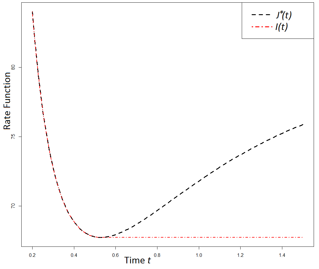
Figure 1: The dotted black line denotes the function $J_{*}(t)$. The dotted red line denotes the rate function $I(t)$. Here $\mu=2.5$, $\beta=1.0$, $x_{0}=4$, $v_{0}=1$ and $t^{o}_{V}\approxeq 0.529$.

Then

$$I(T)\;=\;\inf_{t\in[0,T]}J_{*}(t)\;=\;\left\{\begin{array}[]{ccc}J_{*}(T)&\mbox{ if }&T\leq t^{o}_{V}\\ J_{*}(t^{o})&\mbox{ if }&T>t^{o}_{V}\end{array}\right.\;.$$ (2.27)

Figure 1 illustrates the behavior of the function $J_{*}(t)$ and that of $I(t)$.

Part 3.

We complete the proof by showing that the optimal rate given by (2.27) remains valid even after taking into account the additional path inequality constraint

$$x(s)\geq V(s)\;\;\;\mbox{ for all }s\in[0,t].$$ (2.28)

Define

$$J_{**}(t):=\inf\left\{J(x;t):x\in\mathcal{H}_{x_{0},V(t)}^{1},x(s)\geq V(s)\mbox{ for }s\in[0,t].\right\}$$ (2.29)

Consider the optimal path $x(s)$ of Part 1 given in (2.21) , (2.20), (2.22), for all $s\geq 0$. Note that $c_{2}>0$ (since $\mu>\beta$ and $x_{0}>v_{0}$). The sign of $c_{1}$ depends on $t$: $c_{1}>0\Leftrightarrow v_{0}e^{(\mu+\beta)t}-x_{0}>0$ and this is equivalent to

$$t>t_{1}:=\frac{1}{\mu+\beta}\,\log\frac{x_{0}}{v_{0}}.$$ (2.30)

We also point out that

$$t_{1}<t^{o}_{V}.$$ (2.31)

This follows by the fact that $\phi_{V}$ is a strictly increasing function and

$$\phi_{V}(t_{1})\;=\;\left(1-\frac{\beta}{\mu}\right)e^{(\beta+\mu)t_{1}}+e^{-2\mu t}\frac{\beta}{\mu}e^{(\beta+\mu)t_{1}}\;=\;\frac{x_{0}}{v_{0}}\left(1-\frac{\beta}{\mu}(1-e^{-2\mu t})\right)\;<\;\frac{x_{0}}{v_{0}}=\phi_{V}(t^{o}_{V}).$$

We distinguish three cases according to the relationship between $t$ and $t_{1}$.

Case 1: $t<t_{1}$. This implies that $c_{1}<0$. Because $x(0)>V(0)$, $x^{\prime}(s)=\mu c_{1}e^{\mu s}-\mu c_{2}e^{-\mu s}<0$ for all $s\geq 0$, and $\lim_{s\rightarrow\infty}x(s)=-\infty$, $t$ is the unique intersection point of the paths $x(\cdot)$ and $V(\cdot)$ and the inequality constraint (2.28) is satisfied.

Case 2: $t=t_{1}$. Then, from (2.21) $c_{1}=0$ and $c_{2}=x_{0}$ and hence $x(s)=x_{0}e^{-\mu s}$. Again, the paths $x(\cdot)$ and $V(\cdot)$ intersect only once, at $t$, $x(s)>V(s)$ for $s\in[0,t)$, and the path inequality constraint is satisfied.

Case 3: $t>t_{1}$. Here both $c_{1}>0$ and $c_{2}>0$ and thus $x(s)>0$ for all $s>0$. Therefore, as a result of (2.19), $x^{\prime\prime}(s)>0$ and the function $x$ is strictly convex for all $s\geq 0$. In this case, as is shown in the Appendix, the paths $x(\cdot)$ and $V(\cdot)$ intersect at precisely two points, one of which is of course $t$ while the other will be denoted by $\tau(t)$.

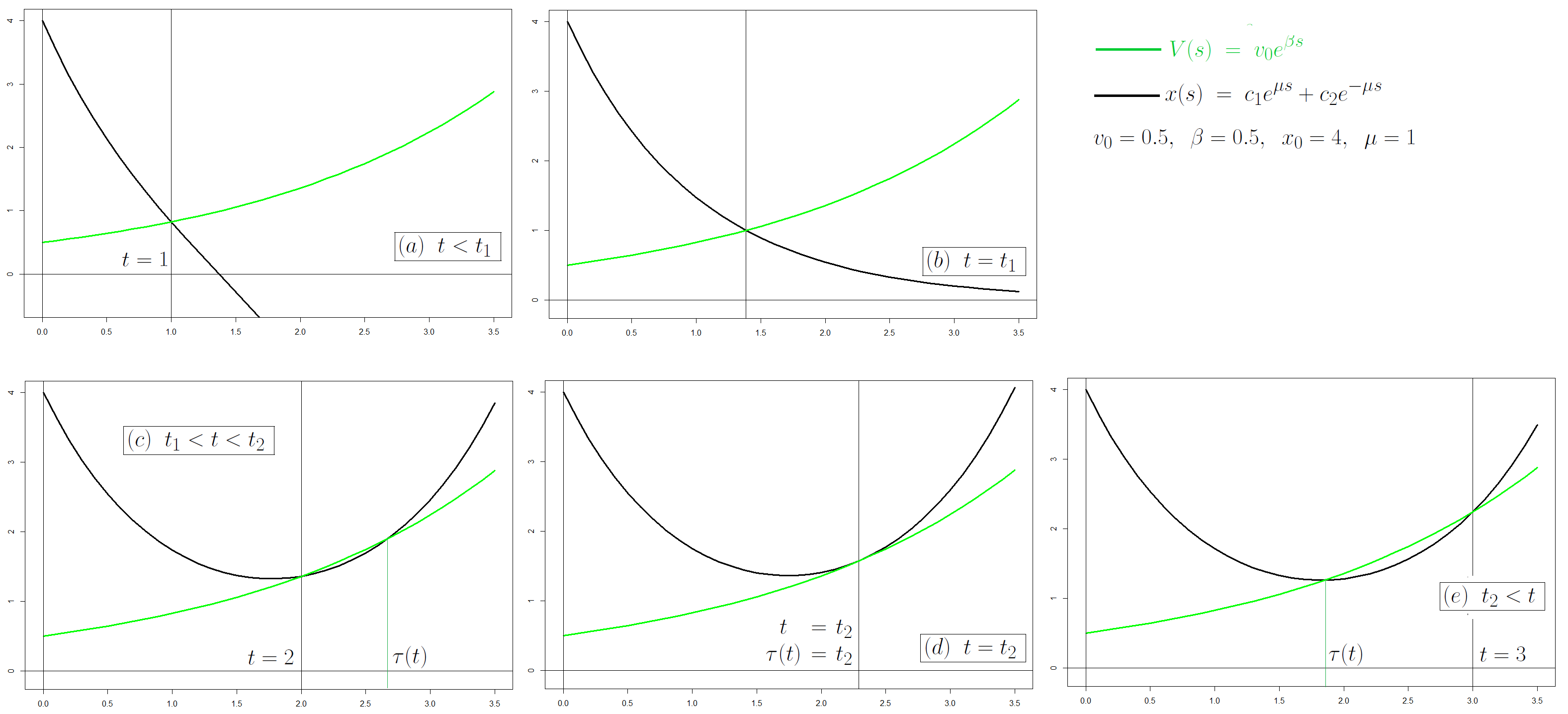
Figure 2: The Three cases. In this example $\mu=1$, $\beta=0.5$, $x_{0}=4$, $v_{0}=0.5$. These give $t_{1}\approx 1.39$ and $t_{2}\approx 2.29$. (a) shows the behavior when $t=1<t_{1}$. This is case 1 and $x(\cdot)$ decreases monotonically. The inequality constraints are satisfied. In (b) $t=t_{1}$. This is case 2 and again the inequality conditions are satisfied. The remaining tree plots illustrate case 3. In (c) and (d) $t\leq t_{2}$ and $\tau(t)\geq t$. Again the inequality constraints are satisfied. In (e) however, when $t>t_{2}$, $\tau(t)<t$ and (2.28) is not satisfied.

Figure 2 shows that for specific values of the parameters $\mu$, $\beta$, $x_{0}$, $v_{0}$. For the values of the parameters in Figure 2 $t_{0}=\frac{1}{2}\log 8\approx 1.04$. Hence in the figure in the left the path $x(s)$ is decreasing and eventually becomes negative. There is a single intersection between the curves $x(s)$ and $V(s)$. On the other hand in the figure in the middle ($t=2$) and in the right ($t=3$) the path $x(s)$ is strictly convex, as is $V(s)$, and thus the two curves intersect in two points. For $t=2$ the path $x(s)$ satisfies (5.9) and therefore (5.6) and (2.28) while for $t=3$ it does not.

The key remark is the following: If $x^{\prime}(t)<V^{\prime}(t)$ then the path $x(\cdot)$ intersects $V(\cdot)$ from above at $t$, then again from below at $\tau(t)>t$. If, conversely, $x^{\prime}(t)>V^{\prime}(t)$ then $x(\cdot)$ intersects $V(\cdot)$ from below at $t$. Since $x(0)>V(0)$ this necessarily implies that there was an earlier crossing from above at $\tau(t)<t$. (The case $x^{\prime}(t)=V^{\prime}(t)$ corresponds to $t=\tau(t)$. The path $x(\cdot)$ is tangent to $V(\cdot)$ at $t$ and $x(s)>V(s)$ for all $s\neq t$.)

The situation in Case 3 is examined in more detailed in Section 5.2 of the Appendix where it is established that there exists a time $t_{2}$ such that $t_{1}<t_{2}$ and the relationship between $t$ and $t_{2}$ determines whether the path $x(\cdot)$ satisfies the inequality constraints (2.28) or not. Specifically

• If $t_{1}<t<t_{2}$ then $x(\cdot)$ intersects $V(\cdot)$ from above at $t$ and hence it satisfies the inequality constraint $x(s)>V(s)$ for $s\in[0,t)$. It crosses $V(t)$ once again at $\tau(t)>t$, this time from below.

• If $t=t_{2}$ then $x(t)$ is tangent to $V(t)$ at $t$. It satisfies the inequality constraint $x(s)>V(s)$ for $s\in[0,t)$ (and in fact even beyond $t$ though this is of no interest for our purposes).

• If $t>t_{2}$ then $x(t)$ crosses $V(t)$ from below. This means that there was a first crossing from above at $\tau(t)<t$. As a result $x(s)<V(s)$ when $s\in(\tau(t),t]$ and the inequality constraint (2.28) is not satisfied in this case.

Figure 3: Here $\mu=1$, $\beta=0.6$, $x_{0}=2$, $v_{0}=0.5$. Thus $t^{o}=0.8664$. The hitting times range from $t=0.25$ to $t=1.50$. Note that, for $t=0.25,\,0.50,$ and $0.75$ the path $x(s)$ eventually becomes negative, after hitting $V(s)$, the thick green line. When the hitting times are greater than $t^{o}$, (i.e. $t=1,\,1.25,\,$ and $1.5$) the path $x(s)$ is a convex function and has two intersection points with the dotted green line.

Figure 3 illustrates these cases. For $t=0.25$, $0.5$, and $0.75$ (black, red, and green paths) the paths eventually become negative and intersect the dotted green line (i.e. the function $V(\cdot)$) once. In the rest of the cases the paths remain positive and intersect the dotted green line twice.

Thus the optimal path of Part 1 also satisfies the constraint (2.28) iff $t\leq t_{2}$. In that case the path given by (2.22) minimizes the functional $J(x,t)$ in (2.16) under the boundary conditions (2.17) and the path inequality constraints (2.28). Then

$$J_{**}(t)=J_{*}(t)\hskip 7.22743pt\mbox{ when }\;t<t_{2}.$$ (2.32)

If $t>t_{2}$ then $t$ is the second point of intersection of $x(s)$ with $V(s)$ and (2.28) is not satisfied. This means that the path $x(s)$ is not feasible under the additional constraint $x(s)>V(s)$ and therefore that the optimal value $J_{*}(t)$ obtained without taking into account the inequality constraint is smaller than $J_{**}(t)$. Thus we have

$$\begin{array}[]{ccc}J_{**}(t)&=&J_{*}(t)\;\mbox{ if }t\leq t_{2}\\ J_{**}(t)&<&J_{*}(t)\;\mbox{ if }t>t_{2}\end{array}$$ (2.33)

Then, the rate function in (2.8), defined as

$$I_{V}(T)\;:=\;\inf\left\{J(x;t):x\in\mathcal{H}_{x_{0},V(t)}^{1},x(s)\geq V(s)\mbox{ for }0<s<t,\;\;0<t\leq T.\right\}$$ (2.34)

can be obtained as

$$I_{V}(T)\;:=\;\min_{t\in(0,T]}J_{**}(t).$$ (2.35)

If $T\leq t_{2}$ then $J_{**}(t)=J_{*}(t)$ and hence $I_{V}(T)=\min_{t\in(0,T]}J_{*}(t)=J_{*}(t^{o}\wedge T)$ due to the fact that $J_{*}$ is strictly decreasing in $(0,t^{o}_{V})$ and strictly increasing in $(t^{o}_{V},\infty)$.

Therefore we conclude that $I_{V}(T)$ is also given by (2.23). This concludes the proof of the first part of Theorem 3. The proof of the second part, pertaining to the upper boundary curve, is similar and will be omitted. ∎

2.3 The infinite horizon problem – lower and upper bound

We now turn to the infinite horizon problem of obtaining a large deviations estimate for the probability $\mathbb{P}(\inf_{t\geq 0}X_{t}-v_{0}e^{\beta t}\leq 0)$ and $\mathbb{P}(\inf_{t\geq 0}X_{t}-u_{0}e^{\alpha t}\geq 0)$ in the same context as that of the previous section. It is of course possible to solve first the corresponding finite horizon problem as we saw in the previous section and then minimize this probability over $T$. Instead of this, we will use here the standard transversality conditions approach of the Calculus of Variations in order to tackle in one step the infinite horizon problem. These are necessary conditions for optimality in variational problems with variable end-points.

Theorem 4.

Suppose $\{X_{t}^{\epsilon}\}$, $\epsilon>0$, is the family of diffusions described by the solution of the SDE (2.5). Suppose also that the upper bounding curve $U(t)=u_{0}e^{\alpha t}$ and lower bounding curve $V(t)=v_{0}e^{\beta t}$ satisfy the inequalities $v_{0}<x_{0}<u_{0}$ and $\beta<\mu<\alpha$. Then

• The probability of ever hitting the lower boundary satisfies

  $$-\lim_{\epsilon\rightarrow 0}\epsilon\log\mathbb{P}\left(\inf_{t\geq 0}X_{t}^{\epsilon}-v_{0}e^{\beta t}\leq 0\right)\;=:\;I_{V}(\infty)\;=\;\frac{x_{0}^{2}\mu}{\sigma^{2}}\,\,\frac{1-e^{-2\mu T_{V}}}{\left(1+\frac{\beta}{\mu-\beta}\,e^{-2\mu T_{V}}\right)^{2}}$$ (2.36)

  and $T_{V}$ is the unique root of equation (2.10). The optimal path $x_{*}$ hitting the lower bound is given by

  $$x_{*}(t)\;=\;x_{0}\frac{e^{-\mu(T_{V}-t)}+\left(\frac{\mu}{\beta}-1\right)e^{\mu(T_{V}-t)}}{e^{-\mu T_{V}}+\left(\frac{\mu}{\beta}-1\right)e^{\mu T_{V}}}.$$ (2.37)

• The probability of ever hitting the upper boundary satisfies

  $$-\lim_{\epsilon\rightarrow 0}\epsilon\log\mathbb{P}\left(\inf_{t\geq 0}X_{t}^{\epsilon}-u_{0}e^{\alpha t}\geq 0\right)\;=\;I_{U}(\infty)\;=\;\frac{x_{0}^{2}\mu}{\sigma^{2}}\,\,\frac{1-e^{-2\mu T_{U}}}{\left(1+\frac{\alpha}{\mu-\alpha}\,e^{-2\mu T_{U}}\right)^{2}}$$ (2.38)

  and $T_{U}$ is the unique root of the equation (2.13). The optimal path hitting the upper bound is given by

  $$x(t)\;=\;x_{0}\,\frac{e^{-\mu(T_{U}-t)}-\left(1-\frac{\mu}{\alpha}\right)e^{\mu(T_{U}-t)}}{e^{-\mu T_{U}}-\left(1-\frac{\mu}{\alpha}\right)e^{\mu T_{U}}}.$$ (2.39)

Proof.

Consider first the problem of hitting the upper boundary at some time $T_{U}$ before hitting the lower boundary. We will obtain low noise logarithmic asymptotics for the probability of hitting the upper boundary (without having first hit the lower). Because in the limit, as $\epsilon\rightarrow 0$, the probability of ever hitting either the upper or the lower boundary goes to 0 exponentially (in $\frac{1}{\epsilon}$) we expect that the presence of the lower boundary (and the stipulation to avoid it) does not affect the probability of hitting the upper boundary.

The optimization problem for the action functional becomes

$$\min\int_{0}^{T_{U}}F(x,x^{\prime},t)dt,\hskip 7.22743pt\mbox{with }F(x,x^{\prime},t)=\frac{1}{2\sigma^{2}}\left(x^{\prime}-\mu x\right)^{2},\hskip 14.45377pt$$ (2.40)

subject to the constraints

$$x(0)=x_{0},\;\;\mbox{ and }x(T_{U})=U(T_{U})$$ (2.41)

$$V(t)<x(t)<U(t)\;\mbox{ for }0\leq t<T_{U},\;\;$$ (2.42)

In the above, both the optimal path $x$ and the horizon $T_{U}$ are unknowns to be determined. Our approach to dealing with the inequality path constraint, (2.42) $x(t)>V(t)$ for all $t\in[0,T)$ will be to initially ignore it and obtain an optimal hitting time $T_{U}$ and an optimal path $x_{*}$ minimizing the criterion (2.40) and satisfying the boundary conditions (2.41). We will then show that this optimal path satisfies the constraints (2.42).

The necessary conditions for a minimum in the problem without the path inequality constraint are

Euler-Lagrange Equation: $$\;\;F_{x}-\frac{d}{dt}F_{x^{\prime}}=0,$$ (2.43)

Boundary Conditions: $$\;\;x(0)=x_{0},\;\;\;x(T_{U})=U(T_{U}),\$$ (2.44)

Transversality Condition: $$\;\;F+(U^{\prime}-x^{\prime})F_{x^{\prime}}=0\;\;\mbox{ at }T_{U}.$$ (2.45)

Taking into account that $F_{x}=-\mu\sigma^{-2}\left(x^{\prime}-\mu x\right)$, $F_{x^{\prime}}=\sigma^{-2}\left(x^{\prime}-\mu x\right)$, $\frac{d}{dt}F_{x^{\prime}}=\sigma^{-2}\left(x^{\prime\prime}-\mu x^{\prime}\right)$, the Euler-Lagrange equation becomes

$$F_{x}-\frac{d}{dt}F_{x^{\prime}}=-\sigma^{-2}\left(x^{\prime\prime}-\mu^{2}x\right)=0$$

and thus

$$x^{\prime\prime}-\mu^{2}x\;=\;0.$$ (2.46)

This has the general solution

$$x(t)=C_{1}e^{\mu t}+C_{2}e^{-\mu t}.$$ (2.47)

Taking into account the boundary conditions (2.44), we obtain

$$x(0) = C_{1}+C_{2}\;=\;x_{0},$$ (2.48)

$$x(T) = C_{1}e^{\mu T_{U}}+C_{2}e^{-\mu T_{U}}\;=\;u_{0}e^{\alpha T_{U}}.$$ (2.49)

The transversality condition (2.45) gives

$$\frac{1}{2\sigma^{2}}\left(x^{\prime}(T_{U})-\mu x(T_{U})\right)^{2}+\left(u_{0}\alpha e^{\alpha T_{U}}-x^{\prime}(T_{U})\right)\frac{1}{\sigma^{2}}\left(x^{\prime}(T_{U})-\mu x(T_{U})\right)\;=\;0$$

or

$$\left(x^{\prime}(T_{U})-\mu x(T_{U})\right)\,\left(-x^{\prime}(T_{U})-\mu x(T_{U})+2u_{0}\alpha e^{\alpha T_{U}}\right)\;=\;0.$$ (2.50)

Taking into account (2.47), it follows that $x^{\prime}(T_{U})-\mu x(T_{U})=-2\mu C_{2}e^{-\mu T_{U}}$ and hence, if the first factor of (2.50) were to vanish, this would imply that $C_{2}=0$. This in turn implies, in view of (2.47), (2.48), and (2.49), that $x(T)=x_{0}e^{\mu T_{U}}=u_{0}e^{\alpha T_{U}}$ which is impossible since $x_{0}<u_{0}$ and $\mu<\alpha$. Hence (2.50) implies

$$u_{0}e^{\alpha T_{U}}\;=\;\frac{\mu}{\alpha}\,C_{1}e^{\mu T_{U}}.$$ (2.51)

From (2.44) and (2.51) we obtain

$$C_{1}+C_{2} = x_{0}$$

$$C_{1}\left(1-\frac{\mu}{\alpha}\right)\,e^{\mu T_{U}}+C_{2}e^{-\mu T_{U}} = 0$$

whence it follows that

$$C_{1}\;=\;\frac{x_{0}e^{-\mu T_{U}}}{\left(\frac{\mu}{\alpha}-1\right)\,e^{\mu T_{U}}+e^{-\mu T_{U}}},\hskip 21.68121ptC_{2}\;=\;\frac{x_{0}\left(\frac{\mu}{\alpha}-1\right)\,e^{\mu T_{U}}}{\left(\frac{\mu}{\alpha}-1\right)\,e^{\mu T_{U}}+e^{-\mu T_{U}}}.$$ (2.52)

From (2.47) and (2.51) we obtain the following equation

$$\left(\frac{\alpha}{\mu}-1\right)\,e^{(\mu+\alpha)T_{U}}\,-\,\frac{\alpha}{\mu}\,e^{(\alpha-\mu)T_{U}}+\frac{x_{0}}{u_{0}}\;=\;0.$$ (2.53)

which must be satisfied by the optimal hitting time $T_{U}$. In fact we will show that this equation has a unique solution, i.e.  $T_{U}$ is the unique solution of (2.13): Indeed, with $\phi_{U}(t)$ as defined in (2.13) we have $\phi_{U}(0)=1$, $\lim_{t\rightarrow\infty}\phi_{U}(t)=-\infty$, and $\phi_{U}^{\prime}(t)=-\frac{\alpha-\mu}{\mu}e^{(\mu+\alpha)t}\left(\mu+\alpha(1-e^{-2\mu t})\right)<0$ for all $t\geq 0$.

An alternative expression for $C_{1}$, $C_{2}$, taking into account (2.53) is

$$C_{1}\;=\;u_{0}\frac{\alpha}{\mu}e^{(\alpha-\mu)T_{U}},\hskip 21.68121ptC_{2}\;=\;u_{0}\left(1-\frac{\alpha}{\mu}\right)e^{(\alpha+\mu)T_{U}}.$$ (2.54)

Using (2.47) and (2.52) we obtain the expression (2.39). If instead we use (2.54) we obtain the alternative expression for the optimal path

$$x(t)\;=\;u_{0}e^{\alpha T_{U}}\left[\frac{\alpha}{\mu}e^{-\mu(T_{U}-t)}-\left(\frac{\alpha}{\mu}-1\right)e^{\mu(T_{U}-t)}\right].$$ (2.55)

From the above we obtain the rate function $I_{U}$ given in (2.38). and hence, on a practical note, the probability that the OU process reaches the upper boundary satisfies approximately

$$\log\mathbb{P}(\sup_{t\geq 0}X_{t}-u_{0}e^{\alpha t}\geq 0)\approx-I_{U}.$$

The quality of this approximation improves as $\sigma$ becomes smaller. Note in particular that the value of $T_{U}$ does not depend on $\sigma$ as is clear from (2.53). Alternative expressions for the rate $I_{U}$, using (2.53) are, of course, possible. For instance,

$$I_{U}\;=\;\frac{\mu}{\sigma^{2}}\frac{\left(u_{0}e^{(\alpha-\mu)T_{U}}-x_{0}\right)^{2}}{1-e^{-2\mu T_{U}}}\;\;=\;\;\frac{\mu}{\sigma^{2}}u_{0}^{2}\left(1-\frac{\mu}{\alpha}\right)^{2}e^{2\alpha T_{U}}\left(e^{2\mu T_{U}}-1\right).$$ (2.56)

There remains to show that the optimal path obtained in (2.55) also satisfies the inequality constraints $v_{0}e^{\beta t}<x(t)<u_{0}e^{\alpha t}$ for $t\in[0,T_{U})$. Indeed

$$x(t)-x_{0}e^{\mu t} = x_{0}\,\frac{e^{-\mu(T_{U}-t)}-\left(1-\frac{\mu}{\alpha}\right)e^{\mu(T_{U}-t)}}{e^{-\mu T_{U}}-\left(1-\frac{\mu}{\alpha}\right)e^{\mu T_{U}}}-x_{0}e^{\mu t}\;=\;\frac{2\left(1-\frac{\mu}{\alpha}\right)e^{\mu T_{U}}\sinh\mu t}{e^{-\mu T_{U}}-\left(1-\frac{\mu}{\alpha}\right)e^{\mu T_{U}}}$$

$$= 2u_{0}\left(\frac{\alpha}{\mu}-1\right)e^{(\mu+\alpha)t}\sinh\mu t\;>\;0\;\;\mbox{ for }t>0.$$

Since $v_{0}e^{\beta t}<x_{0}e^{\mu t}$ for all $t>0$ the above inequality implies $x(t)>v_{0}e^{\beta t}=V(t)$ for $t\in[0,T_{U})$.

Next, define the function $f(t):=u_{0}e^{\alpha t}-x(t)$ for $t\in[0,T_{U}]$. Note that $f(0)=u_{0}-x_{0}>0$ and $f(T_{U})=0$. Also $f^{\prime}(0)=\alpha\left(e^{-\alpha T_{U}}-e^{-\mu T_{U}}\right)-(\alpha-\mu)e^{\mu T_{U}}<0$ (since $\mu<\alpha$). Finally, $f^{\prime\prime}(t)=-\alpha\mu e^{\mu(t-T_{U})}+\alpha^{2}e^{\alpha(t-T_{U})}+\mu(\alpha-\mu)e^{\mu(T_{U}-t)}>0$ for all $t\in[0,T_{U}]$. Thus $f$ is convex on $[0,T_{U}]$ and hence, since $f(T_{U})=0$, the inequality constraint $f(t)>0$ holds on $[0,T_{U}]$ provided that $f^{\prime}(T)<0$. Indeed $f^{\prime}(t)=-\alpha e^{-\mu(t-T_{U})}+\alpha e^{\alpha(t-T_{U})}-(\alpha-\mu)e^{(T_{U}-t)}$ and hence $f^{\prime}(T_{U})=-\alpha+\mu<0$. Therefore the critical path $x(t)$ satisfies the inequality $x(t)<U(t)$ as well, for all $t\in[0,T)$.

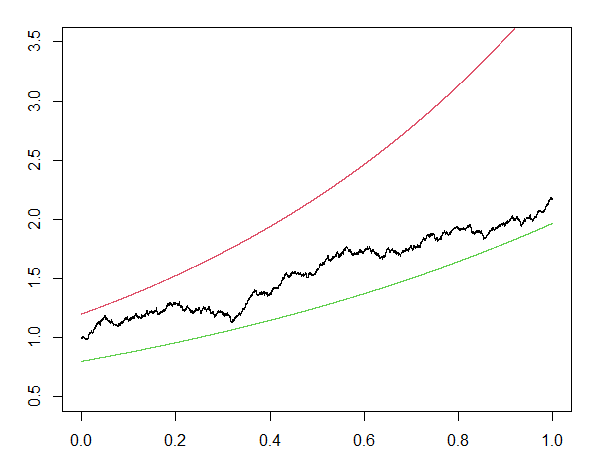
Figure 4: An Ornstein-Uhlenbeck process evolving between an upper and a lower exponential bound.

Intuitively, the uniqueness of the solution of (2.53) makes sense. If $T_{U}$ is very small the noise factor $W_{t}$ must exhibit an extremely unlikely behavior in order for the OU process to rise to the level of the upper curve $U(t)$. So having more time available makes the rare event of hitting the upper boundary more likely. But if $T_{U}$ is too large, because of the difference in the rates of the two processes, again hitting the upper boundary becomes extremely unlikely. Also, in some cases, in the infinite horizon problem, an infimum may exist but no minimum. The rate function $I$ is not ”good” and compactness fails. In practical terms, the more time available the more likely it is that the noise term will cause the diffusion path to hit the deterministic boundary curve.

∎

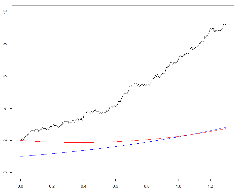
Figure 5: The black line is a typical path of an OU process with $\mu=1$, $\sigma=1$ and starting point $x_{0}=2$. The blue curve is the lower exponential bound $v_{0}e^{\beta t}$ with $v_{0}=1$ and $\beta=0.8$. The meeting $T$ obtained by solving numerically (2.10) is equal to 1.0621. Finally the red optimal (large deviation) path is obtained from (2.37)

In Figures 6, 7, we consider the OU process $dX_{t}=X_{t}+dW_{t}$, with $X_{0}=x_{0}$, (with the value of the parameters $\mu=1$, $\sigma=1$) and the lower and upper bounds $v(t)=0.5e^{0.5t}$, $u(t)=2e^{1.3t}$. (Thus $\alpha=1.3$, $u_{0}=2$, $\beta=0.5$ and $v_{0}=0.5$.) In Figure 5 the optimal value of $T$ that corresponds to the solution of the optimization problems of section 2.3 (equations (2.10) and (2.13)).

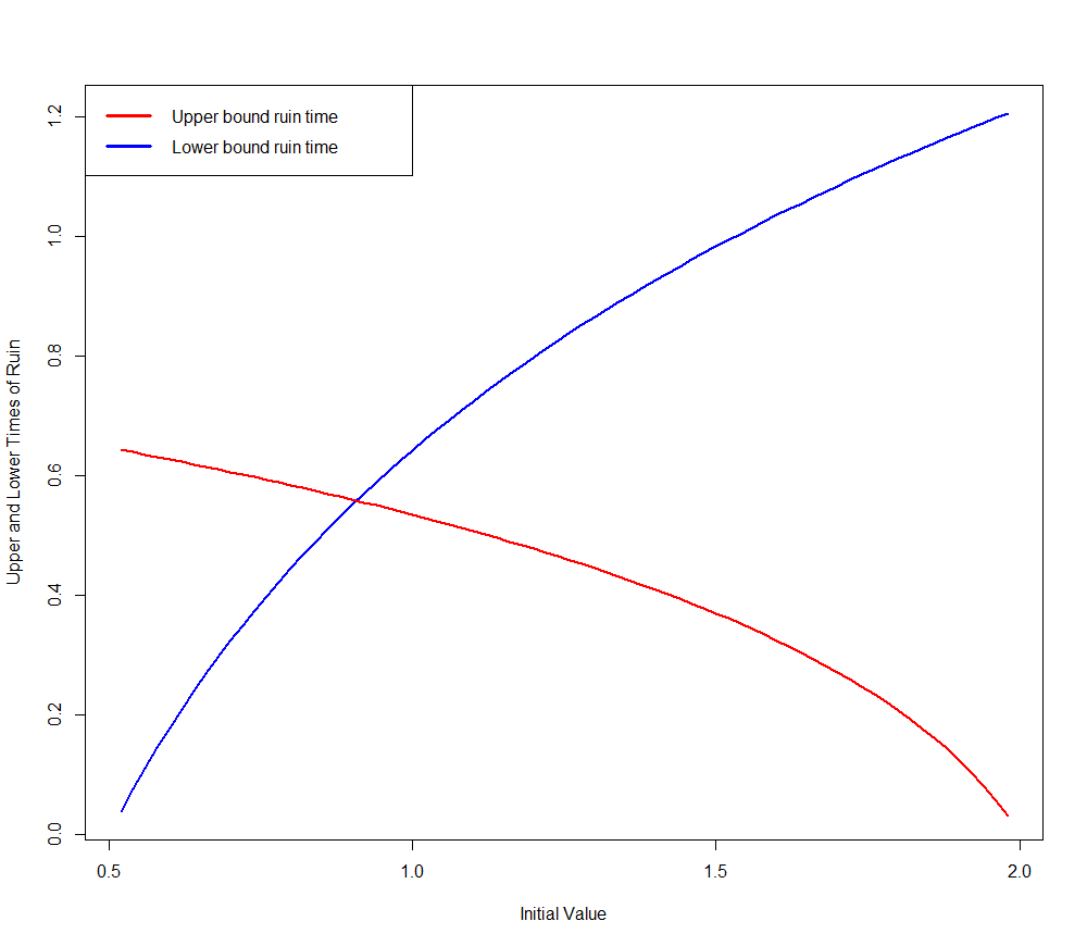
Figure 6: The system under consideration is an OU process with $\mu=1$, $\sigma=1$ and initial position $x_{0}$. The red line is the “optimal hitting time” for the upper curve $u_{0}e^{\alpha t}$ with $u_{0}=2$, $\alpha=1.3$, i.e. the solution of (2.13). Note that this optimal time decreases to zero as $x_{0}$ increases to $u_{0}=2$. Respectively, the blue line is the corresponding ”optimal hitting time” for the lower curve $v_{0}e^{\beta t}$, $\beta=0.5$, $v_{0}=0.5$, i.e. the solution of (2.10). In this case the optimal time increases as the distance of $x_{0}$ from $v_{0}$ increases.

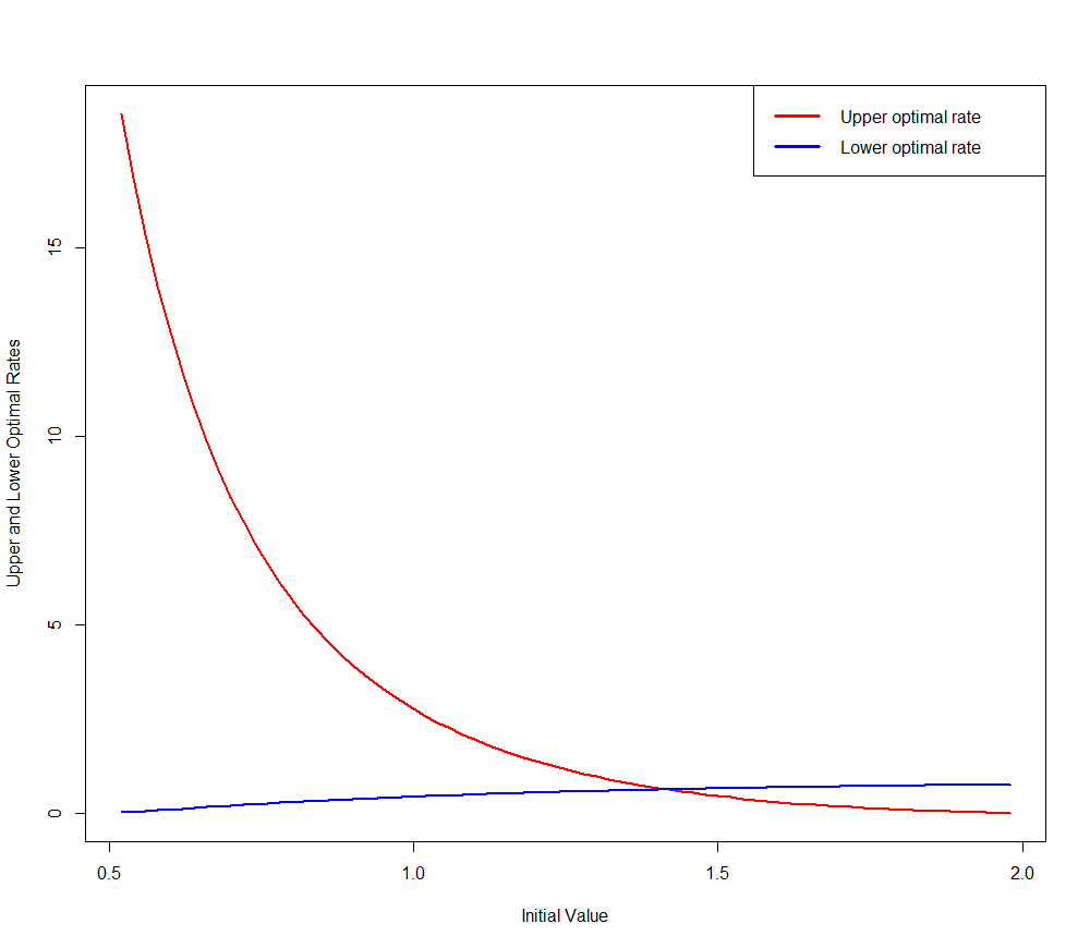
Figure 7: The OU process and the upper and lower curves are as in Figure 6. The red line is a plot of the optimal rate $I_{U}$ for hitting the upper curve in the infinite horizon problem given by (2.38). Correspondingly, the blue line gives the plot of the optimal rate for hitting the lower curve, $I_{V}$, given by (2.36). The point of intersection of the two curves corresponds to the initial condition $x_{0}$ for which the exponential rate for the probability of hitting the upper curve is equal to that for the lower curve.

3 More general models

3.1 Ornstein-Uhlenbeck with a general linear drift

Here we consider the Ornstein-Uhlenbeck process with a more general drift. This is important since it arises as a diffusion approximation in the risk models with interest rates considered in the Introduction. Consider the SDE

$$dX_{t}=(\mu X_{t}+r)dt+\sigma dW_{t},\;\;\;X_{0}=x_{0}.$$

The upper limit is $U(t)=u_{0}e^{\alpha t}$. We assume that $u_{0}>x_{0}$ and $\mu<\alpha$. In the deterministic limit, when $\sigma\rightarrow 0$, one obtains the Ordrinary Differential Equation $\frac{d}{dt}x(t)=\mu x(t)+r$ which has the solution $x(t)=x_{0}e^{\mu t}+\frac{r}{\mu}(e^{\mu t}-1)$. To ensure that we remain in range of applicability of Large Deviation results we will need to ensure that the deterministic solution remains strictly below the upper bound, $U(t)$ for all $t\geq 0$. Let

$$\phi(t)\;:=\;U(t)-x(t)\;=\;u_{0}e^{\alpha t}-\left(x_{0}+\frac{r}{\mu}\right)e^{\mu t}+\frac{r}{\mu}.$$ (3.1)

Then we must have

$$\inf_{t\geq 0}\phi(t)>0.$$ (3.2)

We will make the additional assumption that

$$r\;<\;u_{0}(\alpha-\mu).$$ (3.3)

This assumption ensures that (3.2) holds. Indeed, $\phi(0)=u_{0}-x_{0}>0$ and

$$\phi^{\prime}(t)=e^{\mu t}\left[u_{0}\alpha e^{(\alpha-\mu)t}-x_{0}\mu-r\right].$$

Then,

$$u_{0}\alpha e^{(\alpha-\mu)t}-x_{0}\mu-r\geq u_{0}\alpha-x_{0}\mu-r>u_{0}\alpha-x_{0}\alpha-r>0$$

and hence (3.2) holds.

The action functional is

$$\frac{1}{2\sigma^{2}}\int_{0}^{T}\left(x^{\prime}-\mu x-r\right)^{2}du.$$

The Euler-Lagrange differential equation $F_{x}-\frac{d}{dt}F_{x^{\prime}}=0$ reduces to

$$x^{\prime\prime}-\mu^{2}x-\mu r=0.$$

Its general solution is

$$x(t)=C_{1}e^{\mu t}+C_{2}e^{-\mu t}-\frac{r}{\mu}.$$ (3.4)

The boundary conditions are

$$x_{0} = C_{1}+C_{2}-\frac{r}{\mu}$$ (3.5)

$$u_{0}e^{\alpha T} = C_{1}e^{\mu T}+C_{2}e^{-\mu T}-\frac{r}{\mu}.$$ (3.6)

The transversality condition that must be satisfied by a critical path meeting the curve $U(t):=u_{0}e^{\alpha t}$ at $T$ is

$$F+(U^{\prime}(T)-x^{\prime}(T))F_{x^{\prime}}=0\;\;\mbox{ or }\;\;(x^{\prime}-r-\mu x)\left(-x^{\prime}-r-\mu x+2u_{0}e^{\alpha T}\right)=0$$

which, using (3.4), reduces to

$$C_{2}\left(u_{0}\alpha e^{\alpha T}-\mu C_{1}e^{\mu T}\right)\;=\;0.$$ (3.7)

The above equation leads to the examination of two cases:

Case 1. $C_{2}=0$.

Using this value in (3.5), (3.6), and eliminating $C_{1}$ among them gives

$$u_{0}e^{\alpha T}-\left(x_{0}+\frac{r}{\mu}\right)e^{\mu T}+\frac{r}{\mu}\;=\;0.$$ (3.8)

This equation corresponds to the requirement $\phi(T)=0$ for the function defined in (3.1) which is impossible. Hence $C_{2}=0$ is impossible.

Case 2. $u_{0}\alpha e^{\alpha T}-\mu C_{1}e^{\mu T}=0$.

This, together with (3.6) gives

$$u_{0}\left(1-\frac{\alpha}{\mu}\right)e^{\alpha T}=C_{2}e^{-\mu T}-\frac{r}{\mu}.$$ (3.9)

Using this, (3.5), (3.6), give

$$C_{1}+C_{2} = x_{0}+\frac{r}{\mu}$$ (3.10)

$$C_{1}e^{\mu T}+C_{2}e^{-\mu T} = u_{0}e^{\alpha T}+\frac{r}{\mu}.$$ (3.11)

The above system has the solution

$$C_{1}\;=\;\frac{e^{-\mu T}\left(x_{0}+\frac{r}{\mu}\right)-\left(u_{0}e^{\alpha T}+\frac{r}{\mu}\right)}{e^{-\mu T}-e^{\mu T}},\;\;\;\;C_{2}\;=\;\frac{u_{0}e^{\alpha T}+\frac{r}{\mu}-e^{\mu T}\left(x_{0}+\frac{r}{\mu}\right)}{e^{-\mu T}-e^{\mu T}},$$

Using this, (3.9) reduces to

$$u_{0}\left(\frac{\alpha}{\mu}-1\right)e^{(\alpha+\mu)T}-u_{0}\frac{\alpha}{\mu}e^{(\alpha-\mu)T}-\frac{r}{\mu}e^{\mu T}+x_{0}+\frac{r}{\mu}=0.$$ (3.12)

Under Assumption (3.3) i.e. if the drift term $r$ is either negative or, if positive, not too large the above equation has a unique solution which determines $T$.

Define

$$f(t)=u_{0}\left(\frac{\alpha}{\mu}-1\right)e^{t(\alpha+\mu)}-u_{0}\frac{\alpha}{\mu}e^{(\alpha-\mu)t}-\frac{r}{\mu}e^{\mu t}+x_{0}+\frac{r}{\mu}$$

$$f(0)=x_{0}-u_{0}<0.$$

Also $\lim_{t\rightarrow\infty}f(t)=+\infty$.

$$f^{\prime}(t)=(\alpha+\mu)u_{0}\left(\frac{\alpha}{\mu}-1\right)e^{t(\alpha+\mu)}-u_{0}\frac{\alpha}{\mu}(\alpha-\mu)e^{(\alpha-\mu)t}-re^{\mu t}.$$

$$f^{\prime}(0)=u_{0}(\alpha-\mu)-r.$$

Under the assumption $f^{\prime}(0)>0$. We will show that the condition implies $f^{\prime}(t)>0$ for all $t>0$.

$$e^{-\mu t}f^{\prime}(t)=:g(t)=(\alpha+\mu)u_{0}\left(\frac{\alpha}{\mu}-1\right)e^{\alpha t}-u_{0}\frac{\alpha}{\mu}(\alpha-\mu)e^{(\alpha-2\mu)t}-r$$

$g(0)=f^{\prime}(0)=u_{0}(\alpha-\mu)-r>0$.

$$g^{\prime}(t)=\frac{\alpha}{\mu}e^{\alpha t}(\alpha-\mu)u_{0}\left(\alpha+\mu-(\alpha-2\mu)e^{-2\mu t}\right)>0\;\;\;\mbox{ for all }t\geq 0.$$

This implies the uniqueness of the solution of (3.12).

Then

$$x^{\prime}(T)\;=\;\mu\,\frac{-2(x_{0}+\frac{r}{\mu})+\left(u_{0}e^{\alpha T}+\frac{r}{\mu}\right)\left(e^{\mu T}+e^{-\mu T}\right)}{e^{\mu T}-e^{-\mu T}}.$$ (3.13)

The condition for this solution to satisfy the inequality constraints as well is

$$x^{\prime}(T)>u_{0}\alpha e^{\alpha T}.$$

This is written as

$$\mu\frac{\left(u_{0}e^{\alpha T}+\frac{r}{\mu}\right)\left(e^{\mu T}+e^{-\mu T}\right)-2(x_{0}+\frac{r}{\mu})}{e^{\mu T}-e^{-\mu T}}>\alpha u_{0}e^{\alpha T}.$$

This is equivalent to

$$\frac{r}{\mu}\left(e^{\mu T}+e^{-\mu T}\right)+u_{0}e^{T(\alpha-\mu)}-2(x_{0}+\frac{r}{\mu})>u_{0}e^{\alpha T}\left[\left(\frac{\alpha}{\mu}-1\right)e^{\mu T}-\frac{\alpha}{\mu}e^{-\mu T}\right]\;=\;\frac{r}{\mu}(e^{\mu T}-1)-x_{0}$$

the last equation following from (3.12). Hence

$$\frac{r}{\mu}e^{-\mu T}+u_{0}e^{(\alpha-\mu)T}>x_{0}+\frac{r}{\mu}.$$

This inequality however is true because it is equivalent to $\phi(T)>0$ for the function $\phi$ defined in (3.1), which is true.

The optimal path is in this case

$$x(t)\;=\;\frac{\left(x_{0}+\frac{r}{\mu}\right)\sinh(\mu(T-t))+\left(u_{0}e^{\alpha T}+\frac{r}{\mu}\right)\sinh(\mu t)}{\sinh(\mu T)}-\frac{r}{\mu}.$$

The optimal rate can be obtained from the fact that $x^{\prime}(t)-\mu x(t)-r=2C_{2}e^{\mu t}$ and hence

$$I\;=\;\frac{\mu}{\sigma^{2}}\,\int_{0}^{T}4C_{2}^{2}e^{\mu t}dt\;=\;\frac{\mu}{\sigma^{2}}\,\frac{\left(u_{0}e^{(\alpha-\mu)T}-\frac{r}{\mu}\left(1-e^{-\mu T}\right)-x_{0}\right)^{2}}{1-e^{-2\mu T}}.$$

Note, of course, that when $r\rightarrow 0$ the above reduces to the value of $I$ given in (2.56).

3.2 A Ruin Problem Involving Two Independent OU Processes

Here we generalize the problem examined in the previous section. The lower (or upper) deterministic exponential boundary now is also considered to be stochastic - in fact another, independent, OU process. We may thus study the following pair of SDE’s

$$dX_{t} = \alpha X_{t}dt+\sigma dW_{t},\hskip 21.68121ptX_{0}=x_{0}$$ (3.14)

$$dY_{t} = \beta Y_{t}dt+bdB_{t},\hskip 21.68121ptY_{0}=y_{0}.$$ (3.15)

where $\beta<\alpha$ and $y_{0}<x_{0}$. As a result of these inequalities, in the absence of noise, ($\sigma=b=0$) we would have $Y_{t}<X_{t}$ for all $t$. The presence of noise may cause the two curves to meet however. Again, an exact analysis does not give results in closed form and we obtain low noise logarithmic asymptotics in the Wentzell-Freidlin framework. Using again Theorem 5.6.7 of [3, p. 214] we obtain a two dimensional version of (2.7) for the action functional to be minimized:

$$I\;=\;\int_{0}^{T}F(x,x^{\prime},y,y^{\prime})dt,\hskip 21.68121ptF\;=\;\frac{1}{2}\left[\frac{1}{\sigma^{2}}(x^{\prime}-\alpha x)^{2}+\frac{1}{b^{2}}(y^{\prime}-\beta y)^{2}\right],$$ (3.16)

The boundary conditions $x(0)=x_{0}$, $y(0)=y_{0}$, and $x(T)=y(T)$.

We will again tackle the infinite horizon problem directly and solve the moving boundary variational problem using the appropriate transversality conditions. Thus the first order necessary conditions for an extremum are

$$F_{x}-\frac{d}{dt}F_{x^{\prime}}=0,\hskip 14.45377ptF_{y}-\frac{d}{dt}F_{y^{\prime}}=0$$ (3.17)

$$x(T)=y(T)$$ (3.20)

$$F_{x^{\prime}}+F_{y^{\prime}}=0\;\;\mbox{ at }T,$$

$$F-x^{\prime}F_{x^{\prime}}-y^{\prime}F_{y^{\prime}}=0\;\;\mbox{ at }T.$$

The Euler-Lagrange equations (3.17) give $x^{\prime\prime}-\alpha^{2}x=0$ and $y^{\prime\prime}-\beta^{2}y=0$ and thus, $x(t)=C_{1}e^{\alpha t}+C_{2}e^{-\alpha t}$ and $y(t)=C_{3}e^{\beta t}+C_{4}e^{-\beta t}$ with boundary conditions

$$C_{1}+C_{2}=x_{0},\hskip 14.45377ptC_{3}+C_{4}=y_{0},\hskip 7.22743pt\mbox{and}\hskip 7.22743ptC_{1}e^{\alpha T}+C_{2}e^{-\alpha T}=C_{3}e^{\beta T}+C_{4}e^{-\beta T}.$$ (3.21)

The first transversality condition, (3.20) gives

$$\frac{1}{\sigma^{2}}(x^{\prime}(T)-\alpha x(T))+\frac{1}{b^{2}}(y^{\prime}(T)-\beta y(T))=0$$ (3.22)

or

$$\frac{\alpha}{\sigma^{2}}C_{2}e^{-\alpha T}+\frac{\beta}{b^{2}}C_{4}e^{-\beta T}=0.$$ (3.23)

The second transversality condition (3.20), after routine algebraic manipulations, gives

$$x^{\prime}F_{x^{\prime}}+y^{\prime}F_{y^{\prime}}-F = \frac{1}{2\sigma^{2}}(x^{\prime}-\alpha x)(x^{\prime}+\alpha x)+\frac{1}{2b^{2}}(y^{\prime}-\beta y)(y^{\prime}+\beta y)\;=\;0.$$

The above, in view of (3.22), becomes

$$\left(x^{\prime}(T)-\alpha x(T)\right)\,\left(x^{\prime}(T)+\alpha x(T)-y^{\prime}(T)-\beta y(T)\right)=0.$$

If the first factor is zero then, in view of (3.22), we obtain

$$x^{\prime}(T)-\alpha x(T)=0,\;\;\;y^{\prime}(T)-\beta y(T)=0.$$

In view of the fact that $x^{\prime}(T)-\alpha x(T)=-2\alpha C_{2}e^{-\alpha T}$ this translates into $C_{2}=0$ and similarly $y^{\prime}(T)-\beta y(T)=-2\beta C_{4}e^{-\beta T}=0$ implies $C_{4}=0$. Hence $x(t)=x_{0}e^{\alpha T}$, $y(t)=y_{0}e^{\beta T}$, and $x(T)=y(T)$ implies that $x_{0}e^{\alpha T}=y_{0}e^{\beta T}$ or $e^{(\alpha-\beta)T}=\frac{y_{0}}{x_{0}}$. Since $\alpha-\beta>0$ and $y_{0}/x_{0}<1$ it is impossible to find $T>0$ which satisfies this last equation.

The alternative solution is

$$x^{\prime}(T)+\alpha x(T)\;=\;y^{\prime}(T)+\beta y(T).$$ (3.24)

Note that

$$x^{\prime}(T)+\alpha x(T)=2\alpha C_{1}e^{\alpha T},\;\;\;y^{\prime}(T)+\beta y(T)=2\beta C_{3}e^{\beta T}$$

and hence (3.24) gives

$$\alpha C_{1}e^{\alpha T}\;=\;\beta C_{3}e^{\beta T}.$$ (3.25)

Determination of the optimal path.

Displays (3.21), (3.23), and (3.25) provide the following five equations to determine the five unknown quantities, $C_{i}$, $i=1,\ldots,4$, and $T$:

$$C_{1}+C_{2} = x_{0}$$ (3.26)

$$\frac{\alpha}{\beta}e^{(\alpha-\beta)T}\,C_{1}-\frac{\alpha}{\beta}\,\frac{b^{2}}{\sigma^{2}}e^{-(\alpha-\beta)T}\,C_{2} = y_{0}$$ (3.27)

$$C_{1}e^{\alpha T}+C_{2}e^{-\alpha T} = \frac{\alpha}{\beta}e^{\alpha T}\,C_{1}-\frac{\alpha}{\beta}\,\frac{b^{2}}{\sigma^{2}}e^{-\alpha T}\,C_{2}$$ (3.28)

$$C_{3} = \frac{\alpha}{\beta}e^{(\alpha-\beta)T}\,C_{1}$$ (3.29)

$$C_{4} = -\frac{\alpha}{\beta}\,\frac{b^{2}}{\sigma^{2}}e^{-(\alpha-\beta)T}\,C_{2}$$ (3.30)

From the above we may obtain the values of $C_{i}$, $i=1,\ldots,4$ in terms of $T$:

$$C_{1} = x_{0}\,\frac{\left(1+\frac{\alpha}{\beta}\,\frac{b^{2}}{\sigma^{2}}\right)\,e^{-\alpha T}}{\left(1+\frac{\alpha}{\beta}\,\frac{b^{2}}{\sigma^{2}}\right)\,e^{-\alpha T}+\left(\frac{\alpha}{\beta}-1\right)\,e^{\alpha T}},\;\;\;C_{2}\;=\;x_{0}\,\frac{\left(\frac{\alpha}{\beta}-1\right)\,e^{\alpha T}}{\left(1+\frac{\alpha}{\beta}\,\frac{b^{2}}{\sigma^{2}}\right)\,e^{-\alpha T}+\left(\frac{\alpha}{\beta}-1\right)\,e^{\alpha T}},$$

$$C_{3} = y_{0}\,\frac{\left(1+\frac{\beta}{\alpha}\,\frac{\sigma^{2}}{b^{2}}\right)\,e^{-\beta T}}{\left(1+\frac{\beta}{\alpha}\,\frac{\sigma^{2}}{b^{2}}\right)\,e^{-\beta T}+\left(\frac{\beta}{\alpha}-1\right)\,e^{\beta T}},\;\;\;C_{4}\;=\;y_{0}\,\frac{\left(\frac{\beta}{\alpha}-1\right)\,e^{\beta T}}{\left(1+\frac{\beta}{\alpha}\,\frac{\sigma^{2}}{b^{2}}\right)\,e^{-\beta T}+\left(\frac{\beta}{\alpha}-1\right)\,e^{\beta T}}.$$

From these we obtain the following expression for the critical path

$$x(t) = x_{0}\,\frac{\left(1+\frac{\alpha}{\beta}\,\frac{b^{2}}{\sigma^{2}}\right)\,e^{\alpha(t-T)}\;+\;\left(\frac{\alpha}{\beta}-1\right)\,e^{\alpha(T-t)}}{\left(1+\frac{\alpha}{\beta}\,\frac{b^{2}}{\sigma^{2}}\right)\,e^{-\alpha T}+\left(\frac{\alpha}{\beta}-1\right)\,e^{\alpha T}}$$

$$y(t) = y_{0}\,\frac{\left(1+\frac{\beta}{\alpha}\,\frac{\sigma^{2}}{b^{2}}\right)\,e^{\beta(t-T)}\;+\;\left(\frac{\beta}{\alpha}-1\right)\,e^{\beta(T-t)}}{\left(1+\frac{\beta}{\alpha}\,\frac{\sigma^{2}}{b^{2}}\right)\,e^{-\beta T}+\left(\frac{\beta}{\alpha}-1\right)\,e^{\beta T}}$$

Of course, there remains the task to determine the optimal meeting time $T$. From the above, when $t=T$ we have

$$x(T) = x_{0}\,\frac{\alpha(b^{2}+\sigma^{2})}{(\alpha-\beta)\sigma^{2}e^{\alpha T}+(\beta\sigma^{2}+\alpha b^{2})e^{-\alpha T}},$$

$$y(T) = y_{0}\,\frac{\beta(b^{2}+\sigma^{2})}{(\beta-\alpha)b^{2}e^{\beta T}+(\beta\sigma^{2}+\alpha b^{2})e^{-\beta T}}.$$

At the meeting time $T$, $x(T)=y(T)$ and therefore

$$x_{0}\alpha\left[(\beta-\alpha)b^{2}e^{\beta T}+(\beta\sigma^{2}+\alpha b^{2})e^{-\beta T}\right]\;=\;y_{0}\beta\left[(\alpha-\beta)\sigma^{2}e^{\alpha T}+(\beta\sigma^{2}+\alpha b^{2})e^{-\alpha T}\right]$$ (3.33)

Determination of the meeting time $T$.

We will show that the above equation determines uniquely $T$. To this end, define the function

$$f(t)\;:=\;(\alpha-\beta)\left[y_{0}\beta\sigma^{2}e^{\alpha t}+x_{0}\alpha b^{2}e^{\beta t}\right]+(\beta\sigma^{2}+\alpha b^{2})\left[y_{0}\beta e^{-\alpha t}-x_{0}\alpha e^{-\beta t}\right],\hskip 21.68121ptt\geq 0.$$

It holds that

$$f(0) = (\alpha-\beta)\left[y_{0}\beta\sigma^{2}+x_{0}\alpha b^{2}\right]+(\beta\sigma^{2}+\alpha b^{2})\left[y_{0}\beta-x_{0}\alpha\right]$$

$$= \alpha\beta(\sigma^{2}+b^{2})(y_{0}\beta-x_{0}\alpha)\;<\;0$$

and also $\lim_{t\rightarrow\infty}f(t)=+\infty$. Furthermore

$$f^{\prime}(t)\;=\;(\alpha-\beta)\alpha\beta\left[y_{0}\sigma^{2}e^{\alpha t}+x_{0}b^{2}e^{\beta t}\right]+(\beta\sigma^{2}+\alpha b^{2})\alpha\beta\left[-y_{0}e^{-\alpha t}+x_{0}e^{-\beta t}\right]$$

Clearly $f^{\prime}(t)>0$ for all $t\geq 0$ since $\left[-y_{0}e^{-\alpha t}+x_{0}e^{-\beta t}\right]=e^{-\alpha t}\left[-y_{0}+x_{0}e^{(\alpha-\beta)t}\right]>0$ because $\alpha>\beta$ and $x_{0}>y_{0}$.

$x(t)>y(t)$ when $t\in[0,T)$.

A straight-forward computation (taking into account (LABEL:xt-second), (3.33)) gives

$$x^{\prime}(T)-y^{\prime}(T)\;=\;-\;\frac{x_{0}\alpha(\alpha-\beta)(\sigma^{2}+b^{2})}{(\alpha b^{2}+\beta\sigma^{2})e^{-\alpha T}+\sigma^{2}(\alpha-\beta)e^{\alpha T}}\;<\;0$$ (3.34)

Thus it can be seen that the path $x(\cdot)$ starts above $y(\cdot)$ at 0, crosses it from above at $T$ and (since $\alpha>\beta$) crosses it again once more at some $T^{*}>T$. In particular we note that $x(t)>y(t)$ for $t\in[0,T)$, i.e. $x$ crosses $y$ at $T$ for the first time.

Determination of the rate $I$.

Taking into account that $x^{\prime}(t)-\alpha x(t)=-2\alpha C_{2}e^{-\alpha t}$ and similarly $y^{\prime}(t)-\beta y(t)=-2\beta C_{4}e^{-\beta t}$ the rate function becomes

$$I = \frac{1}{2\sigma^{2}}\int_{0}^{T}4\alpha^{2}C_{2}^{2}e^{-2\alpha t}dt+\frac{1}{2b^{2}}\int_{0}^{T}4\beta^{2}C_{4}^{2}e^{-2\beta t}dt\;=\;\frac{\alpha C_{2}^{2}}{\sigma^{2}}\left(1-e^{-2\alpha T}\right)+\frac{\beta C_{4}^{2}}{b^{2}}\left(1-e^{-2\beta T}\right)$$

$$= \frac{\frac{\alpha}{\sigma^{2}}\left(1-e^{-2\alpha T}\right)x_{0}^{2}\,\left(\frac{\alpha}{\beta}-1\right)^{2}\,e^{2\alpha T}}{\left[\left(1+\frac{\alpha}{\beta}\,\frac{b^{2}}{\sigma^{2}}\right)\,e^{-\alpha T}+\left(\frac{\alpha}{\beta}-1\right)\,e^{\alpha T}\right]^{2}}\;+\;\frac{\frac{\beta}{b^{2}}\left(1-e^{-2\beta T}\right)y_{0}^{2}\left(\frac{\beta}{\alpha}-1\right)^{2}\,e^{2\beta T}}{\left[\left(1+\frac{\beta}{\alpha}\,\frac{\sigma^{2}}{b^{2}}\right)\,e^{-\beta T}+\left(\frac{\beta}{\alpha}-1\right)\,e^{\beta T}\right]^{2}}$$

or equivalently

$$I\;=\;\frac{\alpha(\alpha-\beta)^{2}\sigma^{2}x_{0}^{2}\left(e^{2\alpha T}-1\right)}{\left[(\alpha-\beta)\sigma^{2}e^{\alpha T}+(\beta\sigma^{2}+\alpha b^{2})e^{-\alpha T}\right]^{2}}\;+\;\frac{\beta y_{0}^{2}b^{2}\left(e^{2\beta T}-1\right)\left(\alpha-\beta\right)^{2}}{\left[\left(\alpha b^{2}+\beta\sigma^{2}\right)\,e^{-\beta T}+\left(\beta-\alpha\right)b^{2}\,e^{\beta T}\right]^{2}}.$$ (3.35)

In particular, when $b=0$ and $\alpha=\mu$ then the lower OU process becomes a deterministic lower bound and (3.35) reduces indeed to the right hand side of (2.38), as it should.

Again, as in the proof of Theorem 3 we will show that the solution obtained corresponds to a global minimum using the fact that $F:\mathbb{R}^{4}\rightarrow\mathbb{R}$ is convex and appealing to Theorem 3.16 [2, p.45]. To establish the convexity of $F(x,x^{\prime},y,y^{\prime}):=\frac{1}{2\sigma^{2}}(x^{\prime}-\alpha x)^{2}+\frac{1}{2b^{2}}(y^{\prime}-\beta y)^{2}$ we note that, for any $(x_{0},x_{0}^{\prime},y_{0},y_{0}^{\prime})\in\mathbb{R}^{4}$,

$$F(x,x^{\prime},y,y^{\prime})-F(x_{0},x^{\prime}_{0},y_{0},y^{\prime}_{0})\geq F_{x}^{0}\,(x-x_{0})+F_{x^{\prime}}^{0}\,(x^{\prime}-x^{\prime}_{0})+F_{y}^{0}\,(y-y_{0})+F_{y^{\prime}}^{0}\,(y^{\prime}-y^{\prime}_{0})$$ (3.36)

where $F^{0}_{x}$ is shorthand for $F_{x}(x_{0},x^{\prime}_{0},y_{0},y_{0}^{\prime})$ and similarly for the other three such quantities. The above inequality is equivalent to

$$\frac{1}{2\sigma^{2}}\left(x^{\prime}-\alpha x\right)^{2}+\frac{1}{2b^{2}}\left(x^{\prime}-\beta x\right)^{2}-\frac{1}{2\sigma^{2}}\left(x^{\prime}_{0}-\alpha x_{0}\right)^{2}-\frac{1}{2b^{2}}\left(x^{\prime}_{0}-\beta x_{0}\right)^{2}$$

$$\hskip 72.26999pt\;\geq\;-\frac{\alpha}{\sigma^{2}}\left(x_{0}^{\prime}-\alpha x_{0}\right)\,(x-x_{0})+\frac{1}{\sigma^{2}}\left(x_{0}^{\prime}-\alpha x_{0}\right)\,(x^{\prime}-x^{\prime}_{0})$$

$$\hskip 72.26999pt\;\;\;\;-\frac{\beta}{b^{2}}\left(y_{0}^{\prime}-\beta y_{0}\right)\,(y-y_{0})+\frac{1}{b^{2}}\left(y_{0}^{\prime}-\beta y_{0}\right)\,(y^{\prime}-y^{\prime}_{0}).$$

Elementary algebraic manipulations can show the above inequality to be true and therefore establish inequality (3.36) which implies the convexity of $F$.

We may thus summarize the above long derivation as follows.

Theorem 5.

Consider the pair of Ornstein-Uhlenbeck SDE’s depending on a parameter $\epsilon>0$

$$dX_{t}^{\epsilon} = \alpha X_{t}^{\epsilon}dt+\sqrt{\epsilon}\sigma dW_{t},\hskip 21.68121ptX_{0}^{\epsilon}=x_{0},$$

$$dY_{t}^{\epsilon} = \beta Y_{t}^{\epsilon}dt+\sqrt{\epsilon}bdB_{t},\hskip 21.68121ptY_{0}^{\epsilon}=y_{0}.$$

Assume that $0<y_{0}<x_{0}$ and $0<\beta<\alpha$. Let $T^{\epsilon}:=\inf\{t\geq 0:X_{t}^{\epsilon}=Y_{t}^{\epsilon}\}$ (with the standard convention that $T^{\epsilon}=+\infty$ if the set is empty). Then

$$\lim_{\epsilon\rightarrow 0}\epsilon\log\mathbb{P}(T^{\epsilon}<\infty)\;=\;-I$$

where $I$ is given by (3.35). If this rare event occurs then the meeting path followed by the two processes is given by (LABEL:xt-second) and the meeting time $T$ is the unique solution of (3.33).

4 Geometric Brownian Motion

In this section, an analysis of the problems we examined for the Ornstein-Uhlenbeck process is repeated for the Geometric Brownian motion. The approach followed and the techniques used are analogous to those of section 2. The reason for treating the Geometric Brownian motion in some detail here is due to its great importance in applications but also to the fact that in this case an analytic solution for the types of ruin problems we consider can be obtained. As a result, the accuracy and merit of the large deviation estimates we obtain may be gauged. This is carried out in this section.

4.1 The Finite Horizon Problem

Suppose that $\{X_{t};t\geq 0\}$ is a Geometric Brownian motion satisfying the Stochastic Differential Equation

$$dX_{t}=\mu X_{t}dt+\sigma X_{t}dW_{t},\hskip 21.68121ptX_{0}=x_{0}\;\mbox{w.p. 1.}$$ (4.1)

As is well known this has the closed form solution

$$X_{t}=x_{0}e^{(\mu-\frac{1}{2}\sigma^{2})t+\sigma W_{t}}.$$ (4.2)

Let $u_{0}>x_{0}$ and $\alpha>\mu$. Then the event $\{X_{t}\geq u_{0}e^{at}\mbox{ for some }t\leq T\}$ is an event whose probability goes to 0 as $\sigma\rightarrow 0$. Our goal is to obtain low variance Wentzell-Freidlin asymptotics for this finite horizon hitting probability. For reasons of notational compatibility we introduce the parametrized process

$$dX_{t}^{\epsilon}=\mu X_{t}^{\epsilon}dt+\sqrt{\epsilon}\sigma X_{t}^{\epsilon}dW_{t},\hskip 21.68121ptX_{0}^{\epsilon}=x_{0}\;\mbox{w.p. 1.}$$ (4.3)

Theorem 6.

For the parametrized process $\{X_{t}^{\epsilon}\}$,

$$\lim_{\epsilon\rightarrow 0}\epsilon\log\mathbb{P}\left(\sup_{0\leq t\leq T}\left(X_{t}^{\epsilon}-u_{0}e^{\alpha t}\right)\geq 0\right)\;=\;-I(T).$$ (4.4)

The rate function $I(T)$ is given by

$$I(T):=\min_{0\leq t\leq T}J_{*}(t)$$ (4.5)

where $J_{*}(t)$ is solution to the minimization problem

$$J_{*}(t)\;=\;\min\left\{J(x,t)\;:\;x\in\mathcal{H},\;x(0)=x_{0},\;x(t)=u_{0}e^{\alpha t},\;x(s)<u_{0}e^{\alpha s},\;s\in[0,t)\right\}.$$ (4.6)

where $\mathcal{H}=\left\{h:[0,t]\rightarrow\mathbb{R}:h(s)=h(0)+\int_{0}^{s}\phi(\xi)d\xi\;,\;s\in[0,t],\;\phi\in L^{2}[0,t]\right\}$ and $J(x,t)$ is the action functional

$$J(x,t):=\frac{1}{2}\int_{0}^{t}\left(\frac{x^{\prime}(s)-\mu x(s)}{\sigma x(s)}\right)^{2}ds=\frac{1}{2\sigma^{2}}\int_{0}^{t}\left((\log x(s))^{\prime}-\mu\right)^{2}ds.$$ (4.7)

This theorem is of course a consequence of the Wentzell-Freidlin theory. The minimizing path $x(t)$ can be easily obtained in this case either using the full machinery of the Euler-Lagrange differential equations, or simply by observing that the functional $J(x,t)$ is minimized when $(\log x)^{\prime}$ is constant, say $c$, or equivalently when $\log x(s)=B+cs$ for some $B\in\mathbb{R}$ and $s\in[0,t]$. This in turn implies that $x(s)=Ke^{cs}$ with $x(0)=x_{0}=K$ and $x(t)=x_{0}e^{ct}=u_{0}e^{\alpha t}$ whence we conclude that the function that minimizes the action functional under the boundary conditions is

$$x(t)=x_{0}e^{ct}\hskip 14.45377pt\mbox{where}\;\;\;c=\alpha+\frac{1}{t}\log\frac{u_{0}}{x_{0}}.$$ (4.8)

It is easy to see that the above path satisfies the constraint $x(s)<u_{0}e^{\alpha s}$ for $s\in[0,t)$. The corresponding minimum action is then

$$J_{*}(t)\;=\;\frac{t}{2\sigma^{2}}\left(\alpha-\mu+\frac{1}{t}\log\frac{u_{0}}{x_{0}}\right)^{2}$$

or

$$J_{*}(t)\;=\;t\,\frac{(\alpha-\mu)^{2}}{2\sigma^{2}}+2\frac{(\alpha-\mu)\log\frac{u_{0}}{x_{0}}}{2\sigma^{2}}+\frac{1}{t}\,\frac{(\log\frac{u_{0}}{x_{0}})^{2}}{2\sigma^{2}}.$$

The value of $t$ that minimizes the above expression is

$$t_{\text{min}}=\frac{\log\frac{u_{0}}{x_{0}}}{\alpha-\mu}$$

and the corresponding minimum is

$$\frac{2(\alpha-\mu)\log\frac{u_{0}}{x_{0}}}{\sigma^{2}}.$$

Thus the rate function is

$$I(T)=\left\{\begin{array}[]{lll}\frac{2(\alpha-\mu)\log\frac{u_{0}}{x_{0}}}{\sigma^{2}}&\mbox{if}&t_{\text{min}}<T\\ &&\\ \frac{T}{2\sigma^{2}}\left(\alpha-\mu+\frac{1}{T}\log\frac{u_{0}}{x_{0}}\right)^{2}&\mbox{if}&t_{\text{min}}\geq T\end{array}\right.$$ (4.9)

and, based on Theorem 6, we conclude that

$$-\log\mathbb{P}\left(\sup_{0\leq t\leq T}(X_{t}-u_{0}e^{at})\geq 0\right)\approx I(T).$$ (4.10)

The above approximation is satisfactory provided that $\sigma$ is sufficiently small. We assess its quality in the next subsection taking advantage of the fact that an exact, closed form solution also exists in this situation.

4.2 The exact solution

Consider the GBM $X_{t}=x_{0}e^{(\mu-\frac{1}{2}\sigma^{2})t+\sigma W_{t}}$ and the corresponding finite horizon hitting probability

$$p_{T}\;:=\;\mathbb{P}\left(\sup_{0\leq t\leq T}(X_{t}-u_{0}e^{at})\geq 0\right)$$

where, as before $\alpha>\mu$ and $0<x_{0}<u_{0}$. Since the event $(X_{t}-u_{0}e^{\alpha t})\geq 0$ is the same as $X_{t}e^{-\alpha t}-u_{0}\geq 0$, we will determine, equivalently the probability

$$p_{T} = \mathbb{P}\left(\sup_{0\leq t\leq T}x_{0}e^{(\mu-\frac{1}{2}\sigma^{2}-a)t+\sigma W_{t}}\geq u_{0}\right)\;=\;\mathbb{P}\left(\sup_{0\leq t\leq T}(\mu-\frac{1}{2}\sigma^{2}-\alpha)t+\sigma W_{t}\geq\log\frac{u_{0}}{x_{0}}\right)$$ (4.11)

$$=1-\Phi\left(\frac{\log\left(\frac{u_{0}}{x_{0}}\right)-(\mu-\alpha-\frac{1}{2}\sigma^{2})T}{\sigma\sqrt{T}}\right)$$

$$\hskip 21.68121pt+e^{\frac{2}{\sigma^{2}}(\mu-\alpha-\frac{1}{2}\sigma^{2})\log\left(\frac{u_{0}}{x_{0}}\right)}\Phi\left(\frac{-\log\left(\frac{u_{0}}{x_{0}}\right)-(\mu-\alpha-\frac{1}{2}\sigma^{2})T}{\sigma\sqrt{T}}\right)$$

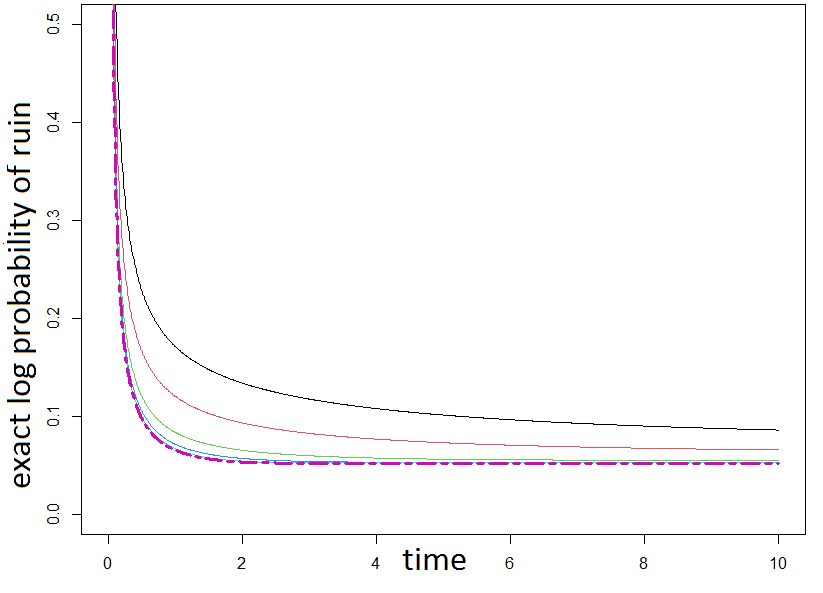
Figure 11: Logarithm of Hitting Probability and Comparison with the Wentzell-Freidlin low variance limit

Here, $\Phi(x):=\int_{-\infty}^{x}\frac{1}{\sqrt{2\pi}}\,e^{-\frac{1}{2}u^{2}}\,du$, the standard normal distribution function. The above exact formula for $p_{T}$ allows us to evaluate the accuracy of the approximation (4.10). Figure 11 shows again $-\sigma^{2}\log p_{T}$ together with the Wentzell-Freidlin asymptotic result when $\sigma\rightarrow 0$. One may see that approximation (4.10) may be considered satisfactory, provided that $\sigma$ is small.

4.3 The Infinite Horizon Problem

The exact value of the infinite horizon hitting probability can be obtained from (4.11) by letting $T\rightarrow\infty$. This gives

$$\lim_{T\rightarrow\infty}p_{T} =: p_{\infty}\;=\;\exp\left(\frac{2}{\sigma^{2}}(\mu-\frac{1}{2}\sigma^{2}-\alpha)\log\frac{u_{0}}{x_{0}}\right).$$

Returning to the parametrized version of the problem, concerning the family of processes $\{X_{t}^{\epsilon}\}$ defined in (4.3), the corresponding infinite horizon hitting probability is

$$p_{\infty}^{\epsilon}\;=\;\exp\left(\frac{2}{\epsilon\sigma^{2}}(\mu-\frac{1}{2}\epsilon\sigma^{2}-\alpha)\log\frac{u_{0}}{x_{0}}\right)$$

and therefore

$$\lim_{\epsilon\rightarrow 0}\epsilon\log p_{\infty}^{\epsilon}\;=\;-\frac{2}{\sigma^{2}}(\alpha-\mu)\log\frac{u_{0}}{x_{0}}.$$ (4.12)

This, as we will see, is the same as the result obtained from Wentzell-Freidlin theory.

Theorem 7.

For the parametrized process $\{X_{t}^{\epsilon}\}$,

$$\lim_{\epsilon\rightarrow 0}\epsilon\log\mathbb{P}\left(\sup_{t\geq 0}\left(X_{t}^{\epsilon}-u_{0}e^{\alpha t}\right)\geq 0\right)\;=\;-I(\infty)$$ (4.13)

where the rate function $I(\infty)$ is the solution to the infinite horizon variational problem

$$\inf\left\{J(x,T)\;:\;x\in\mathcal{H},\;x(s)<u_{0}e^{\alpha s},0\leq s<T,\;x(0)=x_{0},\;x(T)=u_{0}e^{\alpha T}\right\}$$ (4.14)

where $J(x,t):=\frac{1}{2}\int_{0}^{t}\left(\left(\log x(u)\right)^{\prime}-\mu\right)^{2}du$ and $\mathcal{H}$ is again the Cameron-Martin space of absolutely continuous functions with square-integrable derivatives. In fact, the rate function for the infinite horizon problem is

$$I(\infty)=2\frac{\alpha-\mu}{\sigma^{2}}\,\log\frac{u_{0}}{x_{0}},$$ (4.15)

the optimal time horizon is

$$T=\frac{\log\frac{u_{0}}{x_{0}}}{\alpha-\mu},$$ (4.16)

and the optimal path that achives the minimum is

$$x^{*}(t)=x_{0}e^{{2\alpha-\mu}t},\;\;\;t\in[0,T].$$ (4.17)

Figure 8 provides an illustration of the above result.

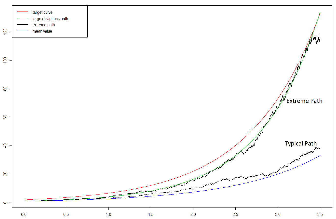
Figure 8: Simulated sample path for $\alpha=1,x_{0}=1,u_{0}=2$ and $\sigma=0.15$. The red curve is the exponential target curve $u_{0}e^{\alpha t}$. The green curve is optimal path predicted by Large Deviations theory and given by $x^{*}(t)=x_{0}e^{(2\alpha-\mu)t}t$. Both a typical path and an extreme path of the Geometric Brownian motion are displayed. The extreme path was generated by simulating a large number of paths ($\approx 10^{5}$) and selecting one that hit the target, i.e. reached the red curve. As expected it follows closely the green curve. The smaller the variance the smaller the probability of hitting the target and the closer the agreement with the theoretical path.

The optimization problem of Theorem 7 can of course be solved using the finite horizon analysis as a basis. However we prefer to use standard techniques of the calculus of variations for infinite horizon problems with the final value of the path constrained to lie on a prescribed curve using the transversality conditions

$$\min\int_{0}^{T}F(x,x^{\prime},t)dt,\hskip 14.45377pt\mbox{ with boundary conditions }x(0)=x_{0},\mbox{ and }x(T)=u(T)$$

$$\mbox{with }F(x,x^{\prime},t)=\frac{1}{2\sigma^{2}}\left(\frac{x^{\prime}}{x}-\mu\right)^{2}.$$ (4.18)

In the above $u(t)=u_{0}e^{\alpha t}$ is a given boundary curve with $x_{0}<u_{0}$ and $x$ is a $C^{1}[0,\infty)$ function which minimizes the “action” integral given the boundary conditions in (4.18). The conditions for a minimum is

$$F_{x}-\frac{d}{dt}F_{x^{\prime}}=0$$ (4.19)

$$x(0)=x_{0}\;\;\;\mbox{ and }\;\;\;x(T)=u(T)$$ (4.20)

$$F+(u^{\prime}-x^{\prime})F_{x^{\prime}}=0\;\;\mbox{ at }T.$$ (4.21)

The first equation is the Euler-Lagrange DE of the Calculus of Variations. Equation (4.21) is known as the transversality condition resulting from the fact that the end time $T$ is not fixed but is itself to be chosen optimally, under the restriction that $x(T)=u(T)$. Then the Euler-Lagrange equation (4.19) becomes

$$\frac{2}{x^{3}}\left((x^{\prime})^{2}-x^{\prime\prime}x\right)=0$$

or equivalently

$$\frac{x^{\prime}}{x}=\frac{x^{\prime\prime}}{x^{\prime}}\;\;\Leftrightarrow\;\;\left(\log x^{\prime}\right)^{\prime}-\left(\log x\right)^{\prime}=0\;\;\Leftrightarrow\;\;\log x^{\prime}-\log x=c_{1}\;\;\Leftrightarrow\;\;\frac{x^{\prime}}{x}=\gamma.$$

Hence

$$x(t)=x_{0}e^{\gamma t}.$$ (4.22)

The transversality condition (4.21) reduces to

$$\left(\frac{x^{\prime}(T)}{x(T)}-\mu\right)\,\left(\frac{x^{\prime}(T)}{x(T)}-\mu+\left(u_{0}\alpha e^{\alpha T}-x^{\prime}(T)\right)\frac{2}{x(T)}\right)=0$$

and taking into account (4.22) we obtain either $\mu=\gamma$ or

$$\gamma-\mu+2\alpha\frac{u_{0}}{x_{0}}e^{(\alpha-\gamma)T}-2\gamma=0$$

or

$$2\alpha\frac{u_{0}}{x_{0}}e^{(\alpha-\gamma)T}=\mu+\gamma.$$ (4.23)

Equation (4.20) gives $x_{0}e^{\gamma T}=u_{0}e^{\alpha T}$ and therefore

$$e^{(\alpha-\gamma)T}=\frac{x_{0}}{u_{0}}.$$ (4.24)

From (4.23) and (4.24) we have

$$\gamma=2\alpha-\mu$$ (4.25)

The solution of the variational process that minimizes the action functional $I$ and satisfies the boundary conditions yields the optimal path $x_{t}=x_{0}e^{(2\alpha-\mu)t}$ and the rate function

$$I=2\frac{\alpha-\mu}{\sigma^{2}}\,\log\frac{u_{0}}{x_{0}}\;\;\mbox{ and }\;\;T=\frac{\log\frac{u_{0}}{x_{0}}}{\alpha-\mu}.$$

It is worth pointing out that, in this case, a closed form analytic expression can also be obtained. The solution of the SDE is $X_{t}^{\epsilon}=x_{0}e^{(\mu-\frac{1}{2}\epsilon\sigma^{2})t+\sqrt{\epsilon}\sigma W_{t}}$ and one may show that

$$\lim_{\epsilon\rightarrow 0}\epsilon\log\mathbb{P}\left(\sup_{t\geq 0}(X_{t}^{\epsilon}-u_{0}e^{\alpha t})\geq 0\right)\\ =-\frac{2}{\sigma^{2}}(\alpha-\mu)\log\frac{u_{0}}{x_{0}}.$$

The exact solution agrees with the Wentzell-Freidlin asymptotic result. In Figure 8 the extreme path was selected by simulating a large number of paths and picking the largest among them.

4.4 Two Correlated Geometric Brownian Motions

Suppose that $W_{t}$, $V_{t}$, are independent standard Brownian motions and $\rho\in[-1,1]$. Set $B_{t}=\rho W_{t}+\sqrt{1-\rho^{2}}\,V_{t}$. Then $(W_{t},B_{t})$ are correlated Brownian motions with correlation $\rho$. Consider now the processes

$$dX_{t} = \alpha X_{t}dt+\sigma X_{t}dW_{t},\hskip 7.22743ptX_{0}=x_{0},$$

$$dY_{t} = \beta Y_{t}dt+bY_{t}dB_{t},\hskip 7.22743ptY_{0}=y_{0}.$$

We will assume that $\alpha>\beta$ and $x_{0}>y_{0}>0$. Thus, in the absence of noise one would have $X_{t}>Y_{t}$ for all $t>0$. In the presence of noise however the probability that $X_{T}=Y_{T}$ for some $T>0$ is non-zero. The second equation can be written equivalently as

$$dY_{t}=\beta Y_{t}dt+\rho bY_{t}dW_{t}+\sqrt{1-\rho^{2}}bY_{t}dV_{t}.$$

Using once more Theorem 5.6.7 of [3, p. 214] we obtain again a two dimensional version of (2.7) for the action functional to be minimized:

$$I=\frac{1}{2}\int_{0}^{T}\left(\frac{x^{\prime}-\alpha x}{x\sigma}\right)^{2}+\frac{1}{1-\rho^{2}}\left(\frac{y^{\prime}-\beta y}{yb}-\rho\frac{x^{\prime}-\alpha x}{x\sigma}\right)^{2}dt$$ (4.26)

This of course can be justified by appealing to the multidimensional version of (2.7) as we have already seen. Set

$$F=\frac{1}{2\sigma^{2}}\left(\frac{x^{\prime}}{x}-\alpha\right)^{2}+\frac{1}{2(1-\rho^{2})}\left(\frac{1}{b}\left(\frac{y^{\prime}}{y}-\beta\right)-\frac{\rho}{\sigma}\left(\frac{x^{\prime}}{x}-\alpha\right)\right)^{2}$$ (4.27)

The conditions for minimum are

$$F_{x}-\frac{d}{dt}F_{x^{\prime}}=0$$ (4.31)

$$F_{y}-\frac{d}{dt}F_{y^{\prime}}=0$$

$$x(T)=y(T)$$

$$F_{x^{\prime}}+F_{y^{\prime}}=0\;\;\mbox{ at }T,$$

$$F-x^{\prime}F_{x^{\prime}}-y^{\prime}F_{y^{\prime}}=0\;\;\mbox{ at }T.$$ (4.32)

Then, after some routine algebraic operations, (4.31) becomes

$$\frac{1}{x}\left[b^{2}\left(\frac{x^{\prime\prime}}{x}-\left(\frac{x^{\prime}}{x}\right)^{2}\right)-\rho b\sigma\left(\frac{y^{\prime\prime}}{y}-\left(\frac{y^{\prime}}{y}\right)^{2}\right)\right]=0$$

which gives $b^{2}(\log x)^{\prime\prime}-\rho b\sigma(\log y)^{\prime\prime}=0$. Similarly (4.31) gives $\sigma^{2}(\log y)^{\prime\prime}-\rho b\sigma(\log x)^{\prime\prime}=0$. These equations together imply that $(\log x)^{\prime\prime}=(\log y)^{\prime\prime}=0$ whence we obtain $\frac{x^{\prime}}{x}=c_{1}$ and $\frac{y^{\prime}}{y}=c_{2}$ for arbitrary $c_{1}$, $c_{2}$, and hence

$$x(t)=x_{0}e^{c_{1}t},\hskip 36.135pty(t)=y_{0}e^{c_{2}t}.$$ (4.33)

Condition (4.31) gives

$$x_{0}e^{c_{1}T}=y_{0}e^{c_{2}T}.$$ (4.34)

Taking into account that $\frac{x^{\prime}}{x}=c_{1}$ and similarly $\frac{y^{\prime}}{y}=c_{2}$, condition (4.31) gives

$$\frac{1}{x_{0}e^{c_{1}T}}\left[b^{2}\left(c_{1}-\alpha\right)-\rho b\sigma\left(c_{2}-\beta\right)\right]+\frac{1}{y_{0}e^{c_{2}T}}\left[\sigma^{2}(c_{2}-\beta)-\rho b\sigma(c_{1}-\alpha)\right]=0$$

Setting $u_{1}=c_{1}-\alpha$, $u_{2}=c_{2}-\beta$, we rewrite the above $b^{2}u_{1}-\rho b\sigma u_{2}+\sigma^{2}u_{2}-\rho b\sigma u_{1}=0$. This gives

$$u_{2}=\lambda u_{1}\;\;\;\mbox{with}\;\;\;\lambda=\frac{b}{\sigma}\frac{\rho\sigma-b}{\sigma-\rho b}$$ (4.35)

Finally, from (4.32),

$$b^{2}u_{1}^{2}+\sigma^{2}u_{2}^{2}-2\rho b\sigma u_{1}u_{2}-2c_{1}\left[b^{2}u_{1}-\rho b\sigma u_{2}\right]-2c_{2}\left[\sigma^{2}u_{2}-\rho b\sigma u_{1}\right]=0$$

or

$$-u_{1}^{2}\left[b^{2}+\sigma^{2}\lambda^{2}-2\rho b\sigma\lambda\right]+2u_{1}\left[-\alpha b^{2}+\beta\rho b\sigma-\lambda\beta\sigma^{2}+\lambda\alpha b\sigma\rho\right]=0.$$

Besides the solution $u_{1}=0$ which means ($c_{1}=\alpha$), we obtain

$$u_{1}=-\frac{2}{b^{2}+\sigma^{2}\lambda^{2}-2\rho b\sigma\lambda}\left(\alpha b^{2}+a\lambda\sigma^{2}-\rho b\sigma(a+\lambda\alpha)\right).$$

After routine algebraic manipulations we obtain

$$u_{1}=2(\beta-\alpha)\frac{\sigma(\sigma-\rho b)}{\sigma^{2}+b^{2}-2\rho b\sigma},\;\;\;\;\;\;\;u_{2}=2(\beta-\alpha)\frac{b(\rho\sigma-b)}{\sigma^{2}+b^{2}-2\rho b\sigma}.$$ (4.36)

From (4.27) and (4.36), together with the definition of $u_{1}$, $u_{2}$,

$$F = \frac{1}{2b^{2}\sigma^{2}(1-\rho^{2})}\left[b^{2}u_{1}^{2}+\sigma^{2}u_{2}^{2}-2\rho b\sigma u_{1}u_{2}\right]\;=\;\frac{2(\beta-\alpha)^{2}}{\sigma^{2}+b^{2}-2\rho b\sigma}.$$ (4.37)

Thus, since

$$T=\frac{1}{\alpha-\beta}\,\log\left(\frac{x_{0}}{y_{0}}\right),$$

the optimal rate is

$$I=\frac{2(\alpha-\beta)\log\left(\frac{x_{0}}{y_{0}}\right)}{\sigma^{2}+b^{2}-2\rho b\sigma}.$$ (4.38)

Figure 9: Two independent Geometric Brownian Motions.

Exact analysis for two correlated Brownian motions

An exact analysis is again possible here. Suppose

$$X_{t}^{\epsilon}\;=\;x_{0}e^{\left(\alpha-\frac{1}{2}\sigma_{\epsilon}^{2}\right)t+\sigma_{\epsilon}W_{t}},\hskip 14.45377ptY_{t}^{\epsilon}\;=\;y_{0}e^{\left(\beta-\frac{1}{2}b_{\epsilon}^{2}\right)t+b_{\epsilon}B_{t}},$$

are two families of Geometric Brownian Motions, indexed by a positive parameter $\epsilon$. We will assume that $\sigma_{\epsilon}=\sigma\sqrt{\epsilon}$ and, similarly, $b_{e}=b\sqrt{\epsilon}$. Assuming that $\alpha>\beta$ and $x_{0}>y_{0}$ and that $\{W_{t}\}$, $\{B_{t}\}$. are standard Brownian motions with correlation $\rho$ as in section 4.4, we are interested in obtaining an expression for the probability

$$\mathbb{P}(T_{\epsilon}<\infty)\;\;\mbox{ where }T_{\epsilon}=\inf\{t>0:Y^{\epsilon}_{t}\geq X^{\epsilon}_{t}\}.$$ (4.39)

The condition $Y^{\epsilon}_{t}\geq X^{\epsilon}_{t}$ is equivalent to

$$\left(\alpha-\beta+\frac{1}{2}(b_{\epsilon}^{2}-\sigma_{\epsilon}^{2})\right)t+\sigma_{\epsilon}W_{t}-b_{\epsilon}B_{t}\leq\log\frac{y_{0}}{x_{0}}.$$

Set $\log\frac{y_{0}}{x_{0}}=-u$, $\gamma_{\epsilon}:=\alpha-\beta+\frac{1}{2}(b_{\epsilon}^{2}-\sigma_{\epsilon}^{2})$ and $\theta_{\epsilon}:=\sqrt{\sigma^{2}_{\epsilon}+b^{2}_{\epsilon}-2\rho b_{\epsilon}\sigma_{\epsilon}}$. If $\{\tilde{W}_{t}\}$ is standard Brownian motion, then (4.39) becomes

$$\mathbb{P}(T_{\epsilon}<\infty)\;=\;\mathbb{P}\left(\inf_{t\geq 0}(\gamma_{\epsilon}t+\theta_{\epsilon}\tilde{W}_{t})<-u\right).$$ (4.40)

Since $\alpha>\beta$, when $\epsilon$ is sufficiently small, $\gamma_{\epsilon}>0$ regardless of the values of $\sigma$ and $b$. Therefore (see [16]) (4.40) becomes

$$\mathbb{P}(T_{\epsilon}<\infty)\;=\;e^{-u\frac{2\gamma_{\epsilon}}{\theta_{\epsilon}^{2}}}\;=\;e^{\log\frac{y_{0}}{x_{0}}\,\frac{2(\alpha-\beta)+(b_{\epsilon}^{2}-\sigma_{\epsilon}^{2})}{\sigma^{2}_{\epsilon}+b^{2}_{\epsilon}-2\rho b_{\epsilon}\sigma_{\epsilon}}}.$$

It therefore follows that

$$\lim_{\epsilon\rightarrow 0}\epsilon\log\mathbb{P}(T_{\epsilon}<\infty)\;=\;\log\frac{y_{0}}{x_{0}}\,\lim_{\epsilon\rightarrow 0}\frac{2(\alpha-\beta)+(b_{\epsilon}^{2}-\sigma_{\epsilon}^{2})}{\epsilon^{-1}\left(\sigma^{2}_{\epsilon}+b^{2}_{\epsilon}-2\rho b_{\epsilon}\sigma_{\epsilon}\right)}\;=\;\log\frac{y_{0}}{x_{0}}\,\frac{2(\alpha-\beta)}{\sigma^{2}+b^{2}-2\rho b\sigma}.$$

This result of course agrees with (4.38).

5 Appendix

5.1 A time-change approach to the Ornstein-Uhlenbeck ruin problem

Consider the two sided problem

$$dX_{t}\;=\;\mu X_{t}dt+\sigma dW_{t},\;\;\;X_{0}=x_{0}$$

with an upper boundary given by the curve $U(t):=u_{0}e^{\alpha t}$ and a lower boundary given by $V(t):=v_{0}e^{\beta t}$. We assume that $0<v_{0}<x_{0}<u_{0}$ and $0<\beta<\mu<\alpha$. We are interested in the hitting time $T=\inf\{t\geq 0:X_{T}\geq U(T)\mbox{ or }X_{T}\leq V(T)\}$. (Of course, if the set is empty, the hitting time is equal to $+\infty$ corresponding to the case where the process never exits from one of the two boundary curves.) The Ornstein-Uhlenbeck process has the solution

$$X_{0}\;=\;x_{0}e^{\mu t}+\sigma\int_{0}^{t}e^{\mu(t-s)}dW_{s}$$

The condition

$$V(t)<X_{t}<U(t)$$

is equivalent to $e^{-\mu t}V(t)<e^{-\mu t}X_{t}<e^{-\mu t}U(t)$ or

$$v_{0}e^{-(\mu-\beta)t}<x_{0}+\sigma\int_{0}^{t}e^{-s\mu}dW_{s}<u_{0}e^{(\alpha-\mu)t}.$$ (5.1)

The stochastic integral $\xi(t):=\sigma\int_{0}^{t}e^{-s\mu}dW_{s}$ is a Gaussian process with independent intervals and variance function

$${\sf Var}(\xi(t))=\sigma^{2}\int_{0}^{t}e^{-2\mu s}ds=\frac{\sigma^{2}}{2\mu}\left(1-e^{-2\mu t}\right).$$

Note that the limit $\lim_{t\rightarrow\infty}{\sf Var}(\xi(t))=\frac{\sigma^{2}}{2\mu}$ is finite. Consider the time change function $\tau(t)$ defined by

$$\tau(t)=\frac{\sigma^{2}}{2\mu}\left(1-e^{-2\mu t}\right),\hskip 21.68121ptt\in[0,\infty)$$ (5.2)

The inverse function (which necessarily exists since ${\sf Var}(\xi(t))$ is an increasing function) is

$$t(\tau)=\log\left(1-\frac{2\mu\tau}{\sigma^{2}}\right),\hskip 21.68121pt\tau\in\left[0,\frac{\sigma^{2}}{2\mu}\right)$$ (5.3)

Applying this change of time to the double inequality (5.1) we obtain

$$v_{0}e^{-(\mu-\beta)\log\left(1-\frac{2\mu\tau}{\sigma^{2}}\right)}<x_{0}+\sigma\int_{0}^{\log\left(1-\frac{2\mu\tau}{\sigma^{2}}\right)}e^{-s\mu}dW_{s}<u_{0}e^{(\alpha-\mu)\log\left(1-\frac{2\mu\tau}{\sigma^{2}}\right)},\hskip 21.68121pt\tau\in\left[0,\frac{\sigma^{2}}{2\mu}\right).$$

However, $\tilde{W}_{\tau}:=\sigma\int_{0}^{\log\left(1-\frac{2\mu\tau}{\sigma^{2}}\right)}e^{-s\mu}dW_{s}$ is standard Brownian motion. (It can easily be seen that it is a continuous martingale with quadratic variation function $\langle\tilde{W}\rangle_{\tau}=\tau$.) Thus we have the equivalent problem

$$v_{0}\left(1-\frac{2\mu\tau}{\sigma^{2}}\right)^{\frac{\mu-\beta}{2\mu}}\;<\;x_{0}\;+\;\tilde{W}_{\tau}\;<\;u_{0}\left(1-\frac{2\mu\tau}{\sigma^{2}}\right)^{-\frac{\alpha-\mu}{2\mu}}\;,\hskip 21.68121pt\tau\in\left[0,\frac{\sigma^{2}}{2\mu}\right).$$ (5.4)

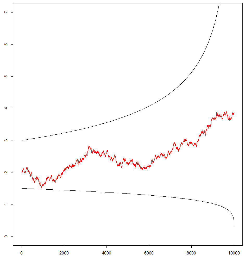
Figure 10: Time-change in an Ornstein-Uhlenbeck ruin problem.

In general, the passage time – hitting probability problem associated with (5.4) must be solved numerically. Of course the time change transformation may have computational advantages. There is a great deal of work, both theoretical and applied, regarding passage times and hitting probabilities of Brownian motion with curving boundaries. In the special case where $\alpha=\beta=\mu$ an exact solution exists. In general we have not been able to obtain closed form expressions even with a single boundary even in the few cases where exact solutions are known, such as for a parabolic boundary: When $\beta=0$ then the time-changed lower bound is $v_{0}\sqrt{1-\frac{2\mu\tau}{\sigma^{2}}}$. While this is a parabolic boundary, the results that have obtained for this case, [23], [24], apply when it acts as an upper and not a lower boundary. Therefore, the exact solution in this case is not known, to the best of our knowledge.

A two–boundary case: $\alpha=\beta=\mu$.

In that case (5.4) becomes

$$v_{0}-x_{0}\;<\;\tilde{W}_{\tau}\;<\;u_{0}-x_{0},\hskip 14.45377pt\tau\in\left[0,\frac{\sigma^{2}}{2\mu}\right).$$

The exact probability of never exiting either boundary, can be obtained from the well known expression for the density of standard Brownian motion (starting at zero) with absorbing boundaries at $a$, $b$, ($a,b>0$). If $p(x,t)dx:=\mathbb{P}\left(W_{t}\in(x,x+dx);\;-b<W_{s}<a,\;0\leq s\leq t\right)$, then, (see [16, p.222])

$$p(x,t) = \sum_{n=1}^{\infty}\frac{2}{a+b}\sin\left(\frac{n\pi b}{a+b}\right)e^{-\lambda_{n}t}\,\sin\left(n\pi\frac{x+b}{a+b}\right),$$

$$\hskip 14.45377pt\mbox{ where }\lambda_{n}=\frac{1}{2}\frac{n^{2}\pi^{2}}{(a+b)^{2}},\;\;n=1,2,\ldots.$$

Then

$$\mathbb{P}\left(-b<W_{s}<a,\;\mbox{ for }0\leq s\leq t\right)=\int_{-b}^{a}p(x,t)dx,$$

and in our case $-b=v_{0}-x_{0}$, $a=u_{0}-x_{0}$, $t=\frac{\sigma^{2}}{2\mu}$. Hence,

$$\mathbb{P}\left(-b<W_{s}<a,\;0\leq s\leq\frac{\sigma^{2}}{2\mu}\right)$$

$$\;=\;\sum_{k=0}^{\infty}\frac{4}{(2k+1)\pi}\exp\left({-\frac{(2k+1)^{2}\pi^{2}\sigma^{2}}{2(u_{0}-v_{0})^{2}\mu}}\right)\sin\frac{(2k+1)\pi(x_{0}-v_{0})}{u_{0}-v_{0}}.$$

5.2 The paths $x(\cdot)$ and $V(\cdot)$.

Here we refer to part 3 of the proof of Theorem 3. The comparison between the slope of the optimal path $x(\cdot)$ and $V(\cdot)$ at the intersection point $t$ is given by the following

Proposition 8.

$$\operatorname{sgn}(x^{\prime}(t)-V^{\prime}(t))=\left\{\begin{array}[]{rcc}-1&\mbox{if}&t<t_{2}\\ 0&\mbox{if}&t=t_{2}\\ +1&\mbox{if}&t>t_{2}\end{array}\right.$$ (5.6)

where $t_{2}$ is the unique solution of the equation $\phi_{2}(t)\;=\;2\frac{x_{0}}{v_{0}}$ with

$$\phi_{2}(s)\;:=\;\left(1-\frac{\beta}{\mu}\right)e^{(\beta+\mu)s}+\left(1+\frac{\beta}{\mu}\right)e^{(\beta-\mu)s}.$$ (5.7)

Also,

$$t_{1}<t^{o}_{V}<t_{2}$$ (5.8)

where $t_{1}$ is defined in (2.30) and $t^{o}_{V}$ in (2.26).

Proof.

Taking into account (2.22), $x^{\prime}(t)-V^{\prime}(t)\;=\;\mu\frac{v_{0}e^{\beta t}\left(e^{\mu t}+e^{-\mu t}\right)-2x_{0}}{e^{\mu t}-e^{-\mu t}}-\beta v_{0}e^{\beta t}$ and hence

$$x^{\prime}(t)-V^{\prime}(t)<0\;\Leftrightarrow\;\left(1-\frac{\beta}{\mu}\right)e^{(\beta+\mu)t}+\left(1+\frac{\beta}{\mu}\right)e^{(\beta-\mu)t}<2\frac{x_{0}}{v_{0}}.$$ (5.9)

Defining the function $\phi_{2}$ via (5.7) we note that $\phi^{\prime}_{2}(s)=(\mu^{2}-\beta^{2})\frac{2}{\mu}e^{\beta s}\sinh(\mu s)>0$ for all $s\geq 0$ and $\phi_{2}(0)=2$. Hence, the equation $\phi_{2}(s)\;=\;2\frac{x_{0}}{v_{0}}$ has a unique, positive solution, say $t_{2}$. Since the function $\phi_{2}(s)$ is continuous and strictly increasing this establishes (5.6).

Next we will show that

$$t^{o}_{V}\;<\;t_{2}.$$ (5.10)

Indeed, using the definition of $\phi_{1}$ and $t^{o}$,

$$\phi_{2}(t^{o}_{V}) = \left(1-\frac{\beta}{\mu}\right)e^{(\beta+\mu)t^{o}_{V}}+\left(1+\frac{\beta}{\mu}\right)e^{(\beta-\mu)t^{o}_{V}}$$

$$= \phi_{1}(t^{o}_{V})\;+\;e^{(\beta-\mu)t^{o}_{V}}<\frac{x_{0}}{v_{0}}+1\;<\;2\frac{x_{0}}{v_{0}}\;=\;\phi_{2}(t_{2}).$$

where we have used the fact that $\beta-\mu<0$ and that $x_{0}>v_{0}$. Then (5.10) follows from the fact that $\phi_{2}$ is increasing.

Finally note that $\phi_{2}(t_{1})=\frac{x_{0}}{v_{0}}\left(1-\frac{\beta}{\mu}+\left(1+\frac{\beta}{\mu}\right)e^{-2\mu t}\right)<2\frac{x_{0}}{v_{0}}$ which implies, since $\phi_{2}$ is strictly increasing, (5.8). ∎

Define the function $h(s):=x(s)-V(s)$. We have $h(0)=x(0)-V(0)=x_{0}-v_{0}>0$. Also $h(t)=x(t)-V(t)=0$. We will show that, when $t>t_{1}$, there are precisely two zeros of the function $h$ on $[0,\infty)$, $t$ and $\tau(t)$. When $t\in(t_{1},t_{2})$ $\tau(t)>t$ whereas when $t>t_{2}$, $\tau(t)<t$. In the special case $t=t_{2}$, $\tau(t_{2})=t_{2}$ is the single zero of $h$ at which $h^{\prime}$ also vanishes.

We have

$$h^{\prime}(s)\;=\;\mu c_{1}e^{\mu s}-\mu c_{2}e^{-\mu s}+\beta v_{0}e^{\beta s}.$$ (5.11)

The following proposition gives some qualitative properties of this function.

Proposition 9.

Suppose $t>t_{1}$. Then there exists $s_{1}(t)>0$ such that $h^{\prime}(s)<0$ when $s<s_{1}(t)$, $h^{\prime}(s_{1})=0$, and $h^{\prime}(s)>0$ when $s>s_{1}(t)$. Also $\lim_{s\rightarrow\infty}h^{\prime}(s)=+\infty$ and the following holds: There are precisely two values for which the function $h$ vanishes. One is $t$ while the second we denote by $\tau(t)$. If $t<s_{1}(t)$ then $\tau(t)>t$ while if $t>s_{1}(t)$ then $\tau(t)<t$. When $t=s_{1}(t)$ then $t=\tau(t)$ and $h(t)=h^{\prime}(t)=0$.

Proof.

First we will show that $h^{\prime}(0)<0$. Indeed,

$$h^{\prime}(0) = \mu(c_{1}-c_{2})-\beta v_{0}\;=\;\mu\;\frac{2v_{0}e^{\beta t}-x_{0}(e^{\mu t}+e^{-\mu t})}{e^{\mu t}-e^{-\mu t}}-\beta v_{0}$$

$$= \frac{2\mu}{e^{2\mu t}-1}\,v_{0}e^{(\beta+\mu)t}-v_{0}\beta-\mu x_{0}\,\frac{e^{2\mu t}+1}{e^{2\mu t}-1}$$

$$= \frac{2\mu}{e^{2\mu t}-1}\,v_{0}\left(e^{(\beta+\mu)t}-1\right)-v_{0}\beta+v_{0}\frac{2\mu}{e^{2\mu t}-1}-\mu x_{0}\,-x_{0}\frac{2\mu}{e^{2\mu t}-1}$$

$$= \frac{\int_{0}^{t}e^{(\beta+\mu)\xi}d\xi}{\int_{0}^{t}e^{2\mu\xi}d\xi}\,(\beta+\mu)v_{0}-v_{0}\beta+v_{0}\frac{2\mu}{e^{2\mu t}-1}-\mu x_{0}\,-x_{0}\frac{2\mu}{e^{2\mu t}-1}$$

The ratio of integrals above is seen to be less than one (since $\beta<\mu$) and hence

$$h^{\prime}(0) \leq (\beta+\mu)v_{0}-v_{0}\beta+v_{0}\frac{2\mu}{e^{2\mu t}-1}-\mu x_{0}\,-x_{0}\frac{2\mu}{e^{2\mu t}-1}$$

$$= (v_{0}-x_{0})\,\left(\mu+\frac{2\mu}{e^{2\mu t}-1}\right)<0.$$

From (5.11) we see that $h^{\prime}(s)=e^{\mu s}h_{1}(s)$ with $h_{1}(s):=\mu c_{1}-\mu c_{2}e^{-2\mu s}+\beta v_{0}e^{-(\mu-\beta)s}$. Clearly $h^{\prime}(s)$ and $h_{1}(s)$ have the same sign. Also, $h_{1}(0)=h^{\prime}(0)<0$ and since $c_{1}>0$, $c_{2}>0$, (the first because $t>t_{2}$) and $\mu>\beta$, it follows that $h_{1}(s)$ is strictly increasing in $s$ and satisfies $h_{1}(s)\uparrow\mu c_{1}>0$ as $s\uparrow\infty$. Therefore there exists a unique $s_{1}>0$ such that $h_{1}(s_{1})=0$.

We have course $h(t)=0$. Since the value of $s_{2}$ determined in Proposition 8 depends on $t$ we will use the notation $s_{2}(t)$. Then,

• If $t\in(t_{1},t_{2})$ then, from Proposition 8, $h^{\prime}(t)<0$ which implies, in view of the above analysis that $s_{2}(t)>t$. This in turn means that $\tau(t)>s_{2}(t)$ and hence that $t<\tau(t)$.

• If $t=t_{2}$ then $h^{\prime}(t_{2})=0$ which implies that $s_{2}(t_{2})=t_{2}$.

• If $t>t_{2}$ then $h^{\prime}(t)>0$ which implies that $s_{2}(t)<t$ and hence that $\tau(t)<s_{2}(t)$. Thus in this case $\tau(t)<t$.

This concludes the proof of the proposition. ∎

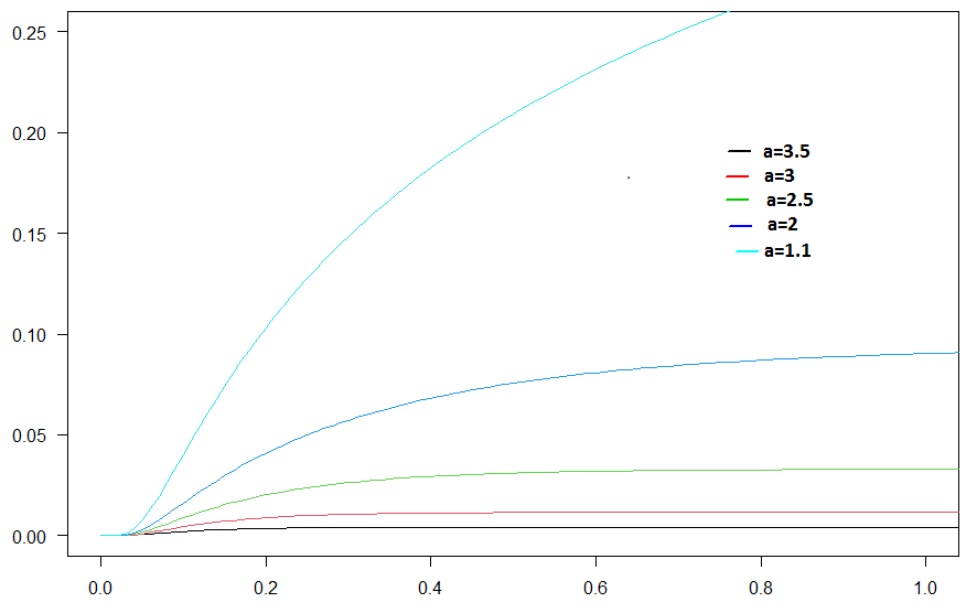
Figure 12: Probability of hitting the upper boundary as a function of time horizon based on the exact solution (4.11). Here $\sigma=0.5$, $x_{0}=1$, $u_{0}=1.3$, $\mu=1$. The function is plotted for $\alpha=1.1$, 2, 2.5, 3, 3.5.

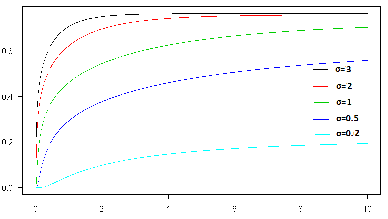
Figure 13: Probability of hitting the upper boundary as a function of time horizon based on the exact solution (4.11). Here $x_{0}=1$, $u_{0}=1.3$, $\mu=1$ $\alpha=1.1$. The function is plotted for $\sigma=0.2$, 0.5, 1, 2, 3.

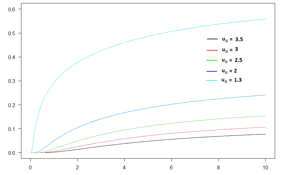
Figure 14: Probability of hitting the upper boundary as a function of time horizon based on the exact solution (4.11). Here $x_{0}=1$, $\alpha=1.1$, $\mu=1$ $\sigma=0.5$. The function is plotted for $u_{0}=1.3$, 2, 2.5, 3, 3.5.

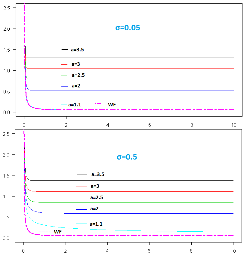
Figure 15: $-log$ Probability of hitting the upper boundary based on the exact solution (4.11). Here $x_{0}=1$, $u_{0}=1.3$, $\mu=1$. The upper graph was obtained for $\sigma=0.05$ while the lower for $\sigma=0.5$. The magenta dotted line gives the value of (the exponent of) the Wentzell-Freidlin approximation.

Figure 16: $-log$ Probability of hitting the upper boundary based on the exact solution (4.11). Here $x_{0}=1$, $\mu=1$, $\alpha=1.3$. The upper graph was obtained for $\sigma=0.05$ while the lower for $\sigma=0.5$. The magenta dotted line gives the value of (the exponent of) the Wentzell-Freidlin approximation.

Figure 17: $-log$ Probability of hitting the upper boundary based on the exact solution (4.11). Here $x_{0}=1$, $u_{0}=1.3$, $\mu=1$, $\alpha=1.1$. The magenta dotted line gives the value of (the exponent of) the Wentzell-Freidlin approximation.

References

- [1] Asmussen, S. and M. Steffensen. 2020. Risk and Insurance, A Graduate Text. Springer.
- [2] U. Brechtken-Manderscheid. 1994. Introduction to the Calculus of Variations. Chapman & Hall.
- [3] A. Dembo and O. Zeitouni. Large Deviations Techniques and Applications. Second Edition. Springer 2010.
- [4] H. U. Gerber and E.S.W. Shiu, “Geometric Brownian Motion Models for Assets and Liabilities: From Pension Funding to Optimal Dividends”, North American Actuarial Journal, 7(3), 37-51, 2003.
- [5] Mark I. Freidlin, Alexander D. Wentzell, Random Perturbations of Dynamical Systems, 3rd edition, Springer Science & Business Media, 2012.
- [6] J. Michael Harrison, “Ruin Problems with Compounding Assets,” Stochastic Processes and their Applications, 5, 67-79, 1977.
- [7] Morton I. Kamien and Nancy L. Schwartz. 1991. Dynamic optimization. The calculus of variations and optimal control in economics and management, 2nd ed. North-Holland.
- [8] Robert S. Maier, Daniel L. Stein, Limiting Exit Location Distributions in the Stochastic Exit Problem SIAM Journal on Applied Mathematics, Vol. 57, No. 3. (Jun., 1997), pp. 752-790.
- [9] P. Baldi, L. Caramellino. General Freidlin–Wentzell Large Deviations and positive diffusions. Statistics and Probability Letters, 81 (2011), 1218-1229.
- [10] Randal G. Williams. The Problem of Stochastic Exit. SIAM J. Appl. Math. 40, 2, 208-223. 1981.
- [11] Alain Simonian. “Asymptotic Distribution of Exit Times for Small-Noise Diffusion.” SIAM J. Appl. Math. 55, 3, 809-826. 1995.
- [12] R. J. Matkowsky and Z. Schuss. “The Exit Problem for Randomly Perturbed Dynamical Systems” SIAM J. Appl. Math. 33, 2, 365-382. 1977.
- [13] Marie Cottrell, Jean-Claude Fort, and Gérard Malgouyres. “Large Deviations and Rare Events in the Study of Stochastic Algorithms.” IEEE Transactions on Automatic Control, AC-28, 9, 907-920. 1983.
- [14] Paolo Baldi. “Exact Asymptotics for the Probability of Exit from a Domain and Applications to Simulation.” The Annals of Probability, 23, 4. 1644-1670, 1995.
- [15] Enzo Olivieri Large Deviations and Metastability. Cambridge University Press, 2005.
- [16] Cox, D.R. and H.D. Miller. The Theory of Stochastic Processes. Chapman and Hall/CRC, 1977.
- [17] Collamore, J.F. “Importance sampling techniques for the multidimensional ruin problem for general Markov additive sequences of random vectors.” The Annals of Applied Probability 12 (1), 382–421, 2002.
- [18] Enid R. Pinch. Optimal Control and the Calculus of Variations. Oxford Science Publications, 1993.
- [19] M. Schilder, Asymptotic formulas for Wiener integrals, Trans. Amer. Math. Soc. 125, 63–85, 1966.
- [20] F. Gao, J. Ren, Large deviations for stochastic flows and their applications, Sci. China Ser. A 44 (8) 1016–1033, 2001.
- [21] Paavo Salminen. On the First Hitting Time and the Last Exit Time for a Brownian Motion to/from a Moving Boundary. Advances in Applied Probability, Vol. 20, No. 2, 411-426, 1988.
- [22] S. Herrmann and E. Tanré. The First-Passage Time of the Brownian Motion to a Curved Boundary: An Algorithmic Approach. SIAM J. SCI. COMPUT. 38, 1, A196–A215. 2016.
- [23] J. Durbin and D. Williams. The First-Passage Density of the Brownian Motion Process to a Curved Boundary. Journal of Applied Probability, 29, 2, 291-304, 1992.
- [24] J. Durbin. The First-Passage Density of a Continuous Gaussian Process to a General Boundary. Journal of Applied Probability, 22, 1, 99-122, 1985.
- [25] Qinglai Dong and Lirong Cui. First Hitting Time Distributions for Brownian Motion and Regions with Piecewise Linear Boundaries. Methodol. Comput. Appl. Probab. 21:1–23, 2019.
- [26] Wendell H. Fleming and Panagiotis E. Souganidis. PDE-viscosity solution approach to some problems of large deviations, Annali della Scuola Normale Superiore di Pisa, Classe di Scienze 4e série, tome 13, no 2, p. 171-192, 1986.
- [27] W.H. Fleming and M.R. James. Asymptotic Series And Exit Time Probabilities. The Annals of Probability, Vol. 20, No. 3, 1369-1384, 1992.
- [28] W.H. Fleming. Exit Probabilities and Optimal Stochastic Control. Applied Mathematics and Optimization, 4. 329-346. 1978.
- [29] Wendell H. Fleming. Stochastic Control for Small Noise Intensities. SIAM J. Control, Vol. 9, No. 3, 473-517, 1971.
- [30] Shuenn-Jyi Sheu. Asymptotic Behavior Of The Invariant Density of a Diffusion Markov Process With Small Diffusion. SlAM J. MATH. ANAL. Vol. 17, No. 2, 451-460, 1986.
- [31] R. Azencott. Petites perturbations aléatoires des systèmes dynamiques: développements asymptotiques. Bulletin des sciences mathématiques, Vol 109, Num 3, pp 253-308, 1985.