A New Perspective On Denoising Based On Optimal Transport

Abstract

In the standard formulation of the classical denoising problem, one is given a probabilistic model relating a latent variable $\Theta\in\Omega\subset\mathbb{R}^{m}\;(m\geq 1)$ and an observation $Z\in\mathbb{R}^{d}$ according to: $Z\mid\Theta\sim p(\cdot\mid\Theta)$ and $\Theta\sim G^{*}$, and the goal is to construct a map to recover the latent variable from the observation. The posterior mean, which is a natural candidate for estimating $\Theta$ from $Z$, attains the minimum Bayes risk (under the squared error loss) but at the expense of over-shrinking the $Z$, and in general may fail to capture the geometric features of the prior distribution $G^{*}$ (e.g., low dimensionality, discreteness, sparsity, etc.). To rectify these drawbacks, in this paper we take a new perspective on this denoising problem that is inspired by optimal transport (OT) theory and use it to propose a new OT-based denoiser at the population level setting. We rigorously prove that, under general assumptions on the model, our OT-based denoiser is mathematically well-defined and unique, and is closely connected to solutions to a Monge OT problem. We then prove that, under appropriate identifiability assumptions on the model, our OT-based denoiser can be recovered solely from information of the marginal distribution of $Z$ and the posterior mean of the model, after solving a linear relaxation problem over a suitable space of couplings that is reminiscent of a standard multimarginal OT (MOT) problem. In particular, thanks to Tweedie’s formula, when the likelihood model $\{p(\cdot\mid\theta)\}_{\theta\in\Omega}$ is an exponential family of distributions, the OT based-denoiser can be recovered solely from the marginal distribution of $Z$. In general, our family of OT-like relaxations is of interest in its own right and for the denoising problem suggests alternative numerical methods inspired by the rich literature on computational OT.

1 Introduction

Consider the following simple latent variable model:

$$Z\mid\Theta=\theta\stackrel{{\scriptstyle}}{{\sim}}p(\cdot\mid\theta)\quad\mbox{and}\quad\Theta\stackrel{{\scriptstyle}}{{\sim}}G^{*},$$ (1.1)

where $\{p(\cdot\mid\theta)\}_{\theta\in\Omega}$ is a known parametric family of probability density functions (p.d.f.’s) on $\mathbb{R}^{d}$ ($d\geq 1$) with respect to (w.r.t.) the Lebesgue measure, and $G^{*}$ is a probability distribution whose support is contained in the set $\Omega$, a subset of $\mathbb{R}^{m}$ for $m\geq 1$. We only get to observe $Z$ from the above model and $\Theta$ is the unobserved latent variable of interest. We denote by $P_{Z,\Theta}$ the joint distribution of $(Z,\Theta)$ on ${\mathbb{R}^{d}}\times\Omega$. By defining a joint distribution over the observable $Z$ and the latent variable $\Theta$, the corresponding distribution of the observed variable is then obtained by marginalization; $Z$ has marginal distribution $\mu$ with density (w.r.t. the Lebesgue measure)

$$f_{G^{*}}(z):=\int p(z\mid\theta)\,dG^{*}(\theta),\qquad\mbox{for }z\in{\mathbb{R}^{d}}.$$ (1.2)

Such latent variable models allow relatively complex marginal distributions to be expressed in terms of more tractable joint distributions over the expanded variable space and thus they provide an important tool for the analysis of multivariate data. Note that (1.1) captures a conceptual framework within which many disparate methods can be unified, including mixture models, factor models, etc; see e.g., Bartholomew et al. (2011). In fact, (1.1) can be thought of as a simple Bayesian model where the prior distribution on $\Theta$ is $G^{*}$. A few important examples of such a setting are given below.

Example 1.1 (Normal location mixture).

Suppose that $p(z\mid\theta)=\varphi_{\sigma}(z-\theta)$ where $\varphi_{\sigma}(\cdot)$ is the p.d.f. of the multivariate normal distribution with mean $0$ and variance $\sigma^{2}I_{d}$ ($\sigma^{2}$ known), i.e., $\varphi_{\sigma}(z):=\frac{1}{(\sqrt{2\pi\sigma^{2}})^{d}}\exp(-\frac{z^{\top}z}{2\sigma^{2}})$, for $z\in\mathbb{R}^{d}$; here $m=d$. If $G^{*}$ is a discrete distribution with finitely many atoms, then $Z$ comes from a finite Gaussian mixture model. This model is ubiquitous in statistics and arises in many application domains including clustering; see e.g., Dempster et al. (1977), McLachlan and Peel (2000).

Example 1.2 (Normal scale mixture).

Suppose that $p(z\mid\theta)=\frac{1}{\theta}\varphi(\frac{z}{\theta})$ where $\varphi(\cdot)$ is the p.d.f. of the standard normal distribution on $\mathbb{R}$. Here $G^{*}$ is a probability distribution on the positive real line $(0,\infty)$. This corresponds to the Gaussian scale mixture model; see Andrews and Mallows (1974). This model has many applications including in Bayesian (linear) regression and multiple hypothesis testing, see e.g., West (1984), Park and Casella (2008), Stephens (2017).

Example 1.3 (Uniform scale mixture).

Suppose that $G^{*}$ is a distribution on $(0,\infty)$ and $p(\cdot\mid\theta)$ corresponds to the uniform density on the interval $[0,\theta]$ (for $\theta>0$). Thus, the marginal density of $Z$ is given by $f_{G^{*}}(z):=\int\frac{1}{\theta}\mathbb{I}_{[0,\theta]}(z)\,dG^{*}(\theta)=\int_{z}^{\infty}\frac{1}{\theta}\,dG^{*}(\theta),$ for $z>0$. It is well-known that any (upper semicontinuous) nonincreasing density on $(0,\infty)$ can be represented as $f_{G^{*}}$ for a suitable $G^{*}$ (Feller, 1971, p. 158). This class of distributions arises naturally via connections with renewal theory (see e.g., Woodroofe and Sun (1993)), multiple testing (see e.g., Langaas et al. (2005), Ignatiadis and Huber (2021)), etc.

We consider the goal of estimating the unobserved $\Theta$ in (1.1); we call this task that of denoising $Z$. Traditionally, this goal has been formulated as that of finding an estimator $\mathfrak{d}^{*}(\cdot)$ that minimizes the Bayes risk w.r.t. a loss function $\ell:\mathbb{R}^{m}\times\mathbb{R}^{m}\to[0,\infty)$, i.e.,

$$\mathbb{E}\left[\ell(\mathfrak{d}(Z),\Theta)\right]\equiv\int_{\Omega}\int_{\mathbb{R}^{d}}\ell(\mathfrak{d}(z),\theta)\,p(z\mid\theta)\,dz\,dG^{*}(\theta)$$ (1.3)

over all measurable functions $\mathfrak{d}:\mathbb{R}^{d}\to\mathbb{R}^{m}$, where $(Z,\Theta)\sim P_{Z,\Theta}$ (i.e., $\Theta\sim G^{*}$ and $Z\mid\Theta=\theta\sim p(\cdot\mid\theta)$). The best estimator $\mathfrak{d}^{*}(Z)$ of $\Theta$, in terms of minimizing (1.3), is called the Bayes estimator under the loss $\ell(\cdot,\cdot)$.

Example 1.4 (Bayes estimator under squared error loss).

When we use the loss function $\ell(a,\theta):=|a-\theta|^{2}$ (here $a,\theta\in\mathbb{R}^{m}$ and $|\cdot|$ denotes the usual Euclidean norm), the Bayes estimator $\overline{\theta}(\cdot)$ minimizing (1.3) turns out to be the posterior mean, i.e.,

$$\overline{\theta}(Z):=\mathbb{E}[\Theta\mid Z].$$ (1.4)

In this paper we take a new perspective on the denoising problem inspired by the theory of optimal transport (OT). To motivate our approach to estimating the unobserved $\Theta$ in (1.1), we first highlight a drawback of the Bayes estimator. Although the posterior mean $\overline{\theta}(Z)\equiv\mathbb{E}[\Theta\mid Z]$ in (1.4) attains the smallest Bayes risk (see (1.3)) among all estimators of $\Theta$ (under the squared error loss), its distribution is different from $G^{*}$ (recall that $\Theta\sim G^{*}$). In fact, in some cases the Bayes estimator $\overline{\theta}(Z)$ yields a ‘shrunken’ estimate of $\Theta$. The left panel of Figure 1 illustrates this with $n=60$ data points $Z_{1},\ldots,Z_{n}$ (denoted by the blue dots) drawn from the model $Z_{i}\mid\Theta_{i}=\theta\sim N(\theta,1)$ where $\Theta_{i}\stackrel{{\scriptstyle iid}}{{\sim}}G^{*}$ with $G^{*}=N(0,\tau^{2})$ and $\tau^{2}=1$. The latent $\Theta_{i}$’s are denoted by red dots, whereas the Bayes estimator $\overline{\theta}(Z_{i})$ is depicted by black dots. We can see that the Bayes estimator (excessively) shrinks the observations in order to achieve optimal denoising (compare the distributions of the red and the black dots). The resulting distribution of the Bayes estimators $\overline{\theta}(Z_{i})$ is $N(0,\frac{1}{2})$, which has a much smaller variance than $G^{*}\equiv N(0,{1})$.

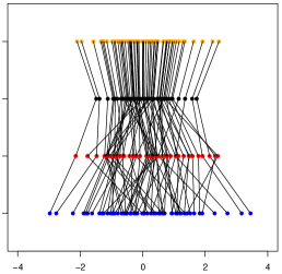
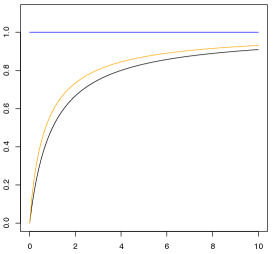
Figure 1: Toy example with $n=60$ in $d=1$ where $p(\cdot\mid\theta)$ is the density of $N(\theta,1)$ and $G^{*}=N(0,\tau^{2})$. Left: Observations $Z_{1},\ldots,Z_{n}$ (in blue) obtained from model (1.1) with $\tau^{2}=1$ are connected to their true unobserved latent variables $\{\Theta_{i}\}_{i=1}^{n}$ (in red); the Bayes estimator $\overline{\theta}(Z_{i})$ (in black) is connected to $\Theta_{i}$ (in red) and the corresponding OT-based denoiser $\delta^{*}(Z_{i})$ (in orange). Right: Plot of the risk curves of the three estimators of $\Theta$ — $Z$ (in blue), $\overline{\theta}(Z)$ (in black) and $\delta^{*}(Z)$ (in orange) — as $\tau^{2}$ varies from 0 to 10.

In contrast, we propose in this paper the OT-based denoiser $\delta^{*}(Z)$ (see (2.9)), shown in the left plot of Figure 1 by the orange dots, which corrects this drawback and produces estimates that have the distribution $G^{*}$; compare the distributions of the orange and the red dots. The plot of the risk functions for the three estimators — $Z$, $\overline{\theta}(Z)$ and $\delta^{*}(Z)$ — as $\tau^{2}$ varies show that the proposed OT-based denoiser $\delta^{*}(Z)$ achieves the distributional stability (i.e., $\delta^{*}(Z)\sim G^{*}$) at very little cost; compare the risk functions for $\delta^{*}(Z)$ (in orange) and $\overline{\theta}(Z)$ (in black). See Remark 2.3 for the detailed computations.

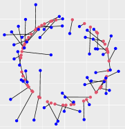
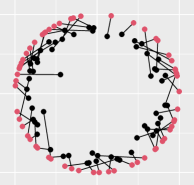
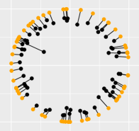
Figure 2: Toy example with $n=60$ in $d=2$ where $p(\cdot\mid\theta)$ is the density of $N(\theta,(0.3)^{2}\cdot I_{2})$ and $G^{*}$ is the uniform distribution on the unit circle. Left: Observations $Z_{1},\ldots,Z_{n}$ (in blue) obtained from model (1.1) are connected to the corresponding unobserved latent variables $\{\Theta_{i}\}_{i=1}^{n}$ (in red). Center: The Bayes estimator $\overline{\theta}(Z_{i})$ (in black) is connected to $\Theta_{i}$ (in red), for every $i=1,\ldots,n$. Right: The Bayes estimator $\overline{\theta}(Z_{i})$ (in black) is connected to its corresponding OT-based denoiser $\delta^{*}(Z_{i})$ (in orange) lying on the circle.

This (over)-shrinkage by the Bayes estimator $\overline{\theta}(Z)$ is more acute when $d\geq 2$. In general, the Bayes estimator $\overline{\theta}(Z)$ is not necessarily guaranteed to lie ‘close’ to $\text{spt}(G^{*})$, the support of $G^{*}$ (recall that $\Theta\sim G^{*}$). To illustrate this, in Figure 2 we consider another example, this time with $d=m=2$. Here we take $n=60$ data points $Z_{1},\ldots,Z_{n}\in\mathbb{R}^{2}$ (depicted by the blue dots in the left panel of Figure 2) drawn from the normal location mixture model (Example 1.1) with the latent variables $\Theta_{1},\ldots,\Theta_{n}$ drawn uniformly on the circle of radius 1 (shown by the red dots in the left panel of Figure 2). We connect $Z_{i}$ with $\Theta_{i}$ by a black line, for each $i=1,\ldots,n$, in the plot. The middle panel of Figure 2 shows the Bayes estimator at the observed data points $\overline{\theta}(Z_{i})$ (depicted by the black dots) connected to the corresponding $\Theta_{i}$’s (in red). As can be easily seen from this plot, the Bayes estimator shrinks most of the observations towards $0\in\mathbb{R}^{2}$. In contrast, our proposed OT-based denoiser corrects this drawback and maps the Bayes estimator $\overline{\theta}(Z_{i})$ to $\delta^{*}(Z_{i})$ (shown in the right panel of Figure 2 by orange dots) which lies on the circle. Note that $\delta^{*}(Z_{i})$, by definition, takes values in $\text{spt}(G^{*})$, the support of $G^{*}$.

In fact, if the goal is to estimate $\Theta\sim G^{*}$, it is reasonable to restrict $\mathfrak{d}(\cdot)$ in (1.3) to all estimators such that $\mathfrak{d}(Z)$ is distributed (approximately) as $G^{*}$. This requirement is particularly important when we believe that $G^{*}$ is discrete with a few atoms (which corresponds to the clustering problem) or when we believe that $G^{*}$ has ‘structure’ (e.g., supported on a lower dimensional manifold in $\mathbb{R}^{m}$). In light of this discussion, it is natural to seek solutions to

$$\inf_{\delta:\mathbb{R}^{d}\rightarrow\mathbb{R}^{m}}\mathbb{E}_{(Z,\Theta)\sim P_{Z,\Theta}}\left[|\delta(Z)-\Theta|^{2}\right]\qquad\mbox{subject to }\;\;\delta(Z)\sim G^{*},$$ (1.5)

among all measurable functions $\delta:{\mathbb{R}^{d}}\to\mathbb{R}^{m}$, where we consider $\ell(\cdot,\cdot)$ to be the squared error loss for simplicity; see Appendix D for a discussion on more general loss functions. The constraint $\delta(Z)\sim G^{*}$ ensures that the ‘estimator’ $\delta(Z)$ of $\Theta$ has the same distribution as $G^{*}$ (in particular, the same support as $\Theta\sim G^{*}$), thereby addressing the above drawbacks; cf. (1.3). This discussion leads to the following natural questions:

1. Under what conditions can it be guaranteed that there exist solutions to problem (1.5)? Are these solutions unique?

2. If there exists a solution, how can one find it? In particular, is it possible to obtain it solely from the marginal distribution of observations and knowledge of the likelihood model?

The purpose of this paper is to provide answers to the above questions in the population level setting that has been discussed up to this point. In this process, we lay down the needed mathematical foundations for future implementation of our ideas in finite data settings.

Our first main result, Theorem 2.4, states that, under certain assumptions on the model, problem (1.5) indeed possesses a unique solution $\delta^{*}(\cdot)$. What is more, this solution can be found by solving an OT problem (defined precisely in (2.10)) between the distribution of the Bayes estimator $\overline{\theta}(Z)$ and $G^{*}$. We refer to this $\delta^{*}(\cdot)$ as the OT-based denoiser associated to the model $(\{p(\cdot\mid\theta)\}_{\theta\in\Omega},G^{*})$. Problem (1.5) can also be interpreted as an extreme case in a family of problems with a soft penalty defined according to

$$\inf_{\delta:{\mathbb{R}^{d}}\rightarrow\mathbb{R}^{m}}\mathbb{E}_{(Z,\Theta)\sim P_{Z,\Theta}}\left[|\delta(Z)-\Theta|^{2}\right]+\frac{1}{2\tau}W_{2}^{2}(\delta_{\sharp}\mu,G^{*}),$$ (1.6)

where $\tau>0$ is a tuning parameter, $\delta_{\sharp}\mu$ is the pushforward of $\mu$ by $\delta$ (i.e., the distribution of $\delta(Z)$ if $Z\sim\mu$; see Definition 2.1) and $W_{2}(\cdot,\cdot)$ denotes the $2$-Wasserstein distance between probability distributions (see Definition 2.3). Formally, when $\tau\rightarrow\infty$ we recover the standard unconstrained risk minimiziation problem, whose solution is the Bayes estimator, whereas we recover problem (1.5) when $\tau\rightarrow 0$. For any other value of $\tau$ in between these two extremes, Theorem 2.5 guarantees that the solution to (1.6) is unique and can be explicitly written as a simple linear interpolation of the OT-based denoiser $\delta^{*}(\cdot)$ and the Bayes estimator $\overline{\theta}(\cdot)$. We will refer to (1.6) as a latent space penalization approach to denoising, given that the penalty term $W_{2}^{2}(\delta_{\sharp}\mu,G^{*})$ involves an explicit comparison of distributions in the latent space $\Omega\subset\mathbb{R}^{m}$.

Although the characterization of the OT-based denoiser $\delta^{*}(\cdot)$ as a solution to an OT problem is appealing, in many real applications $G^{*}$ may be unknown, making this characterization difficult to implement. One possible approach to go around this issue is to estimate $G^{*}$ using i.i.d. data from (1.1) using tools from what is usually referred to in statistics as deconvolution (see e.g., Carroll and Hall (1988), Zhang (1990), Fan (1991), Meister (2009)). This approach is also taken in the empirical Bayes literature; see e.g., Robbins (1956a), Jiang and Zhang (2009), Efron (2011a), Efron (2019), Soloff et al. (2021), as well as the brief discussion on this topic that we present in Appendix E. In this paper, however, we offer a different approach and study yet another formulation for the denoising problem that closely resembles (1.6) but where we directly work with $\mu$, the (marginal) distribution of the observed data (see (1.2)). Indeed, we consider the optimization problem:

$$\inf_{\delta:{\mathbb{R}^{d}}\to\mathbb{R}^{m}}\mathcal{E}_{\tau}(\delta):=\mathbb{E}_{(Z,\Theta)\sim P_{Z,\Theta}}[|\delta(Z)-\Theta|^{2}]+\frac{1}{2\tau}W_{2}^{2}(\mu_{\delta},\mu);$$ (1.7)

here, for a given map $\delta$ we define $\mu_{\delta}$ as the probability measure over $\mathbb{R}^{d}$ defined as

$$\mu_{\delta}(A):=\int_{A}\int_{{\mathbb{R}^{d}}}p(z^{\prime}\mid\delta(z))\,d\mu(z)\,dz^{\prime},\quad\forall A\subseteq\mathbb{R}^{d}\text{ Borel measurable}.$$ (1.8)

In words, $\mu_{\delta}$ is the marginal distribution of the variable $z$ assuming that the underlying distribution of the latent variable $\theta$ is given by $G=\delta_{\sharp}\mu$. We will refer to (1.7) as an observable space penalization approach to denoising, given that the penalty term $W_{2}^{2}(\mu_{\delta},\mu)$ involves an explicit comparison of distributions in the observable space $\mathbb{R}^{d}$. In Proposition 3.1 we show that, under suitable assumptions, the objective function $\mathcal{E}_{\tau}$ (in (1.7)) is Fréchet differentiable w.r.t. the target $\delta\in\mathbb{L}^{2}({\mathbb{R}^{d}}:\mathbb{R}^{m};\mu)$ and provide an explicit formula for its gradient (see (3.1)). The formula for the gradient, which can be easily adapted to the empirical setting, can be used to implement a first order optimization method seeking a solution for (1.7). Unfortunately, problem (1.7) is non-convex in $\delta$ and thus one cannot guarantee the convergence of a steepest descent scheme towards a global minimizer of $\mathcal{E}_{\tau}(\cdot)$. In fact, even the existence of global solutions to (1.7) is not guaranteed by straightforward arguments in the calculus of variations. The main technical difficulty for this is the lack of lower semicontinuity of the functional $\delta\mapsto W_{2}^{2}(\mu_{\delta},\mu)$ w.r.t. the weak topology in the Hilbert space $\mathbb{L}^{2}({\mathbb{R}^{d}}:\mathbb{R}^{m};\mu)$ (see Definition C.1), a natural topology where one can guarantee pre-compactness of minimizing sequences.

Despite the above discussion, we can prove that indeed there exist solutions to (1.7); see Theorem 3.4. This is achieved by considering a suitable relaxation argument where we “lift” the original problem (1.7) to a problem over couplings (see (3.4) for details) that, while not of a standard type in OT theory, does resemble multimarginal optimal transport (MOT) problems. Like MOT problems, our relaxation is linear, and its search space enjoys better compactness properties than the original problem (1.7) that in particular can be used to prove existence of solutions (see Theorem 3.3). This relaxation, which we show is exact under suitable assumptions, also motivates the use of computational tools in OT for constructing solutions of (1.7); this will be explored in future work. Finally, we highlight that this relaxation is the key mathematical construction that allows us to prove Theorem 3.6, which states that, under the identifiability assumptions on the probabilistic model that are written down precisely in Assumption 3.5, the solutions $\delta_{\tau}^{*}$ of (1.7) converge, as $\tau\rightarrow 0$, to the OT-based denoiser $\delta^{*}$; in Remark 3.7 we discuss the non-identifiable case.

As we discuss in Section 6, in order to use the relaxation problem (3.4) to approximate $\delta^{*}$ from finitely many observations, one would first need to estimate $\overline{\theta}(\cdot)$ from the available data. This is where Tweedie’s formula (see (B.5) in Appendix B) can be very useful. This formula expresses the posterior mean $\overline{\theta}(\cdot)$ in an exponential family model (see Appendix A.1) in terms of the marginal density $f_{G^{*}}$ of the observations (and its gradient) only, and can thus be estimated (nonparametrically) directly from observations $Z_{1},\ldots,Z_{n}$, say via kernel density estimation. We thus anticipate to be able to construct consistent estimators for $\delta^{*}$ without knowing $G^{*}$ explicitly or having to directly estimate it, at least in the case when the likelihood model is an exponential family of distributions.

1.1 Outline

The rest of the paper is organized as follows. In Section 2 we present our main results on problems (1.5) and (1.6). First, in Section 2.1 we introduce some necessary notation and background that we use in the rest of the paper. Then, in Section 2.2 we state our first main result, Theorem 2.4, which establishes the existence and uniqueness of solutions of (1.5). In Section 2.3 we state Theorem 2.5, which characterizes the solution of the soft penalty problem (1.6). Section 3 is devoted to the observable space penalization problem (1.7). First, we provide a characterization of the Frechét derivative of its objective under suitable differentiability assumptions on the likelihood model. Then we present Theorems 3.4 and 3.6, where, respectively, we state the existence of solutions to (1.7) and characterize the behavior of solutions to (1.7) as the parameter $\tau$ goes to zero. In particular, Theorem 3.6 states that, under suitable identifiability assumptions, the OT-based denoiser $\delta^{*}$ can be recovered as a limit of solutions to (1.7). Sections 4 and 5 are devoted to the proofs of our main results from Sections 2 and 3, respectively. In Section 6, the conclusions section, we discuss some future directions for research stemming from this work.

In Appendices A-E we provide various discussions connected to our main results. In particular, in Appendices A-B we introduce exponential families of distributions and describe Tweedie’s formula. In Appendix C we state and prove a few results from measure theory and functional analysis that are relevant to the proof of Theorem 3.6. Appendix D briefly describes OT formulations of (1.5) when using more general loss functions (beyond the squared error loss). In Appendix E we briefly review the (nonparametric) maximum likelihood estimator of $G^{*}$, which could potentially be used to implement (1.5) in practical settings.

2 Denoising with latent space penalization

2.1 Preliminaries

We first introduce some definitions and notation from the theory of OT (see e.g., Villani (2003, 2009)). For any metric space $\mathcal{X}$, let $\mathfrak{B}(\mathcal{X})$ denote the set of all Borel measurable subsets of $\mathcal{X}$, and let $\mathcal{P}(\mathcal{X})$ be the set of all Borel probability measures over $\mathcal{X}$. It will be convenient to first introduce the notion of pushforward of a measure by a map and rewrite the constraint in (1.5) in terms of pushforwards.

Definition 2.1 (Pushforward of a measure).

Given a measurable map $\delta:\mathcal{X}\rightarrow\mathcal{Y}$ and a probability measure $\nu$ over $\mathcal{X}$, the measure $\delta_{\sharp}\nu$, the pushforward of $\nu$ by $\delta$, is the measure defined according to $\delta_{\sharp}\nu(A):=\nu(\delta^{-1}(A))$ for every Borel subset $A$ of $\mathcal{Y}$. In other words, if $X\sim\nu$, then $\delta(X)\sim\delta_{\sharp}\nu$.

Remark 2.1.

The constraint $\delta(Z)\sim G^{*}$ in (1.5) can be rewritten as $\delta_{\sharp}\mu=G^{*}$.

Let two probability measures $\nu,\widetilde{\nu}$ be defined over two Polish spaces $\mathcal{X}$ and $\mathcal{Y}$, and consider a lower semicontinuous cost function $c:\mathcal{X}\times\mathcal{Y}\to[0,\infty]$. The dual of the Kantorovich OT problem (see e.g., Villani (2003, 2009))

$$C(\nu,\widetilde{\nu}):=\min_{\pi\in\Gamma(\nu,\widetilde{\nu})}\int\int c(x,y)\,d\pi(x,y),$$ (2.1)

where $\Gamma(\nu,\widetilde{\nu})$ denotes the set of all Borel probability measures on the product $\mathcal{X}\times\mathcal{Y}$ with marginals $\nu$ and $\widetilde{\nu}$ (a.k.a. couplings between $\nu$ and $\widetilde{\nu}$), is the problem

$$\sup_{\phi,\psi}\int\phi(x)\,d\nu(x)+\int\psi(y)\,d\widetilde{\nu}(y),\;\;\text{s.t. }\phi(x)+\psi(y)\leq c(x,y),\;\;\nu\text{-a.e.\leavevmode\nobreak\ }x\in\mathcal{X},\;\widetilde{\nu}\text{-a.e.\leavevmode\nobreak\ }y\in\mathcal{Y},$$ (2.2)

where $\phi$ and $\psi$ are, respectively, in $\mathbb{L}^{1}(\mathcal{X},\nu)$ and $\mathbb{L}^{1}(\mathcal{Y},\widetilde{\nu})$. Theorem 5.10 in Villani (2009) guarantees that primal and dual problems are equivalent. Any solution pair $(\phi,\psi)$ of (2.2), if it exists, will be referred to as optimal dual potentials for the OT problem (2.1).

We will often consider the setting where the space $\mathcal{X}$ is a subset of some Euclidean space, $\mathcal{X}=\mathcal{Y}$, and $c(x,y)=|x-y|^{2}$. When in this setting, we will refer to (2.1) as the $2$-OT problem between $\nu$ and $\widetilde{\nu}$ and denote by $W_{2}^{2}(\nu,\widetilde{\nu})$ the minimum value in (2.1), which is nothing but the square of the so-called Wasserstein distance between $\nu$ and $\widetilde{\nu}$.

Definition 2.2 ($2$-Wasserstein distance).

Given two probability measures $\nu,\widetilde{\nu}$ over $\mathbb{R}^{p}$ with finite second moments, we define their Wasserstein distance $W_{2}(\nu,\widetilde{\nu})$ as

$$W_{2}^{2}(\nu,\widetilde{\nu}):=\min_{\pi\in\Gamma(\nu,\widetilde{\nu})}\int|x-y|^{2}\,d\pi(x,y).$$ (2.3)

A landmark result in the theory of OT due to Brenier characterizes the optimal coupling $\pi$ for the $2$-OT problem between two measures $\nu$ and $\widetilde{\nu}$ when $\nu$ is absolutely continuous w.r.t. the Lebesgue measure; see e.g., Villani (2009, Theorem 3.15).

Theorem 2.1 (Brenier).

Let $\nu$ and $\widetilde{\nu}$ be two Borel probability measures over $\mathbb{R}^{p}$ such that $\int|x|^{2}\,d\nu(x)<\infty$ and $\int|y|^{2}\,d{\widetilde{\nu}}(y)<\infty$. Suppose further that $\nu$ has a Lebesgue density. Then there exists a convex function $\psi:\mathbb{R}^{p}\to\mathbb{R}\cup\{+\infty\}$ whose gradient $T=\nabla\psi$ pushes $\nu$ forward to $\widetilde{\nu}$. In fact, there exists only one such $T$ that arises as the gradient of a convex function, i.e., $T$ is unique $\nu$-a.e. Moreover, $T$ uniquely minimizes Monge’s problem:

$$\inf_{T\>:\>T_{\sharp}\nu=\widetilde{\nu}}\int|x-T(x)|^{2}d\nu(x)$$

and the coupling $(\mathrm{Id}\times T)_{\sharp}\nu$ uniquely minimizes (2.3). In the above and in the remainder of the paper, the map $(\mathrm{Id}\times T):\mathbb{R}^{p}\to\mathbb{R}^{p}\times\mathbb{R}^{p}$ is defined as $(\mathrm{Id}\times T)(x)=(x,T(x))$.

2.2 Rewriting (1.5) as an optimal transport problem

In this subsection we study problem (1.5) and develop its connection with standard Monge and Kantorovich OT problems with a suitable cost function. Thanks to Remark 2.1, problem (1.5) can be written as

$$\min_{\delta\>:\>\delta_{\sharp}\mu=G^{*}}\mathbb{E}_{(Z,\Theta)\sim P_{Z,\Theta}}\left[|\delta(Z)-\Theta|^{2}\right].$$ (2.4)

In turn, problem (2.4) is equivalent to:

$$\min_{\delta\>:\>\delta_{\sharp}\mu=G^{*}}\mathbb{E}_{Z\sim\mu}\left[|\delta(Z)-\overline{\theta}(Z)|^{2}\right],$$ (2.5)

where

$$\overline{\theta}(z):=\mathbb{E}_{(Z,\Theta)\sim P_{Z,\Theta}}\left[\Theta\mid Z=z\right]$$ (2.6)

is the posterior mean (and the Bayes estimator under the quadratic loss). This equivalence follows from the well-known bias-variance decomposition for the squared error loss:

$$\mathbb{E}[|\delta(Z)-\Theta|^{2}\mid Z]=\mathbb{E}[|\delta(Z)-\overline{\theta}(Z)|^{2}\mid Z]+\mathbb{E}[|\overline{\theta}(Z)-\Theta|^{2}\mid Z],$$

which implies that for any arbitrary $\delta:{\mathbb{R}^{d}}\rightarrow\mathbb{R}^{m}$ we have

$$\mathbb{E}_{(Z,\Theta)\sim P_{Z,\Theta}}\left[|\delta(Z)-\Theta|^{2}\right]=\mathbb{E}_{Z\sim\mu}[|\delta(Z)-\overline{\theta}(Z)|^{2}]+\mathbb{E}_{(Z,\Theta)\sim P_{Z,\Theta}}[|\overline{\theta}(Z)-\Theta|^{2}],$$

from where it follows that the objective in (2.4) is equal to the objective function in (2.5) up to the constant $R_{\text{Bayes}}:=\mathbb{E}_{(Z,\Theta)\sim P_{Z,\Theta}}[|\overline{\theta}(Z)-\Theta|^{2}]$, i.e., the Bayes risk.

The advantage of problem (2.5) is that, as discussed below, it is amenable to the type of relaxation methods that have been studied in OT theory. Indeed, in order to construct a solution to (2.5) (and thus also to (2.4)), at least for certain families of models $(\{p(\cdot\mid\theta)\}_{\theta\in\Omega},G^{*})$ satisfying suitable assumptions, we will first consider a Kantorovich relaxation of (2.5) given by

$$\min_{\pi\in\Gamma(\mu,G^{*})}\iint c_{G^{*}}(z,\vartheta)\,d\pi(z,\vartheta),$$ (2.7)

where the cost function $c_{G^{*}}(\cdot,\cdot)$ is defined as

$$c_{G^{*}}(z,\vartheta):=|\overline{\theta}(z)-\vartheta|^{2},\quad(z,\vartheta)\in{\mathbb{R}^{d}}\times\Omega;$$ (2.8)

note the dependence of $G^{*}$ on the cost function $c_{G^{*}}(z,\vartheta)$ in (2.8) via the Bayes estimator $\overline{\theta}(z)$, which depends on $G^{*}$.

We make the following assumptions.

Assumption 2.2.

The distribution $G^{*}$ is such that $\int_{\Omega}|\vartheta|^{2}dG^{*}(\vartheta)<\infty$, i.e., $G^{*}$ has finite second moments.

Assumption 2.3.

The measure $\overline{\theta}_{\sharp}\mu$ is absolutely continuous w.r.t. the Lebesgue measure in $\mathbb{R}^{m}$.

Remark 2.2 (On our assumptions).

Since $\mu$ is absolutely continuous w.r.t. the Lebesgue measure (recall (1.2)), note that Assumption 2.3 holds if we assume that the map $\overline{\theta}:\mathbb{R}^{d}\rightarrow\mathbb{R}^{m}$ is locally-Lipschitz (and thus differentiable Lebesgue a.e.) and that the Jacobian matrix $D\overline{\theta}(z)\in\mathbb{R}^{d\times m}$ has full rank $\mu$-a.e. $z$; indeed, this implication follows from the so called coarea formula (see e.g., the theorem in Section 3.1 in Federer (1959)). Thus, implicitly, we would be assuming that $d\geq m$. In particular, the above is satisfied for the following scenario. If $\{p(\cdot\mid\theta)\}_{\theta\in\Omega}$ is a regular $k$-parameter exponential family in canonical form, then $\overline{\theta}(\cdot)$ is the gradient of a convex function $\kappa(\cdot)$ (which happens to be the log-partition function of the family); see Section A.1 and Appendix B. Moreover, $\kappa(z)$ is a strictly convex function of $z$ on its domain if the representation is minimal; see e.g., Wainwright and Jordan (2008, Proposition 3.1). As convex functions are a.e. twice continuously differentiable, the Jacobian matrix $D\overline{\theta}(z)\in\mathbb{R}^{d\times m}$ exists a.e., and thus Assumption 2.3 is automatically satisfied. Assumption 2.2 just assumes a finite second moment condition on $G^{*}$, which is quite mild.

We are ready to state our first main result.

Theorem 2.4.

Under Assumptions 2.2 and 2.3, there exists a unique solution $\pi^{*}$ to problem (2.7) with cost function (2.8), which takes the form

$$\pi^{*}=(\mathrm{Id}\times\delta^{*})_{\sharp}\mu$$

for a map $\delta^{*}(\cdot)$ that is the unique solution to problem (2.4), i.e., it is the OT-based denoiser. Furthermore, $\delta^{*}(\cdot)$ can be written as

$$\delta^{*}(z)=\nabla\varphi^{*}(\overline{\theta}(z)),\qquad\mbox{for }\;\;z\in{\mathbb{R}^{d}},$$ (2.9)

to be read: “the gradient of the function $\varphi^{*}$ evaluated at $\overline{\theta}(z)$”, where $\varphi^{*}:\mathbb{R}^{m}\rightarrow\mathbb{R}\cup\{+\infty\}$ is a convex function. In fact, $T^{*}:=\nabla\varphi^{*}$ is the solution to the standard quadratic cost Monge OT problem

$$\min_{T:T_{\sharp}({\overline{\theta}}_{\sharp}\mu)=G^{*}}\int|\theta-T(\theta)|^{2}\,d\overline{\theta}_{\sharp}\mu(\theta)$$ (2.10)

between the measures $\overline{\theta}_{\sharp}\mu$ and $G^{*}$.

The proof of Theorem 2.4 is presented in Section 4. It builds upon Brenier theorem (Theorem 2.1). The first part of Theorem 2.4 implies that, under Assumptions 2.2 and 2.3, the value of Kantorovich’s relaxation problem in (2.7) is indeed the same as that of Monge’s problem (2.4). Further, the optimal coupling in (2.7) yields the solution to (2.4). Theorem 2.4 further says that the optimal solution $\delta^{*}(\cdot)$ of (2.4) is related to the Bayes estimator (2.6); in fact, $\delta^{*}(\cdot)$ pushes the Bayes estimator $\overline{\theta}(\cdot)$ to satisfy the distributional constraint $\delta^{*}(Z)\sim G^{*}$. The fact that $\delta^{*}(\cdot)$ has such a simple form is not immediately obvious from the original formulation of the problem in (1.5).

Remark 2.3 (Normal-normal location model).

Suppose that $d=m$ and $\Theta\sim N_{m}(\theta^{*},\Sigma^{*})$ and $Z\mid\Theta=\theta\sim N_{d}(\theta,\Sigma)$, where $\theta^{*}\in\mathbb{R}^{m}$ is known, and $\Sigma^{*}\in\mathbb{R}^{m\times m}$ and $\Sigma\in\mathbb{R}^{d\times d}$ are symmetric positive definite (fixed) matrices. It is then well-known that

$$\overline{\theta}(Z)=\Sigma^{*}(\Sigma^{*}+\Sigma)^{-1}Z+\Sigma(\Sigma^{*}+\Sigma)^{-1}\theta^{*}$$

which shows that

$$\overline{\theta}(Z)\sim N_{m}\Big{(}\theta^{*},A\Big{)},\qquad\mbox{where }\;\;A:=\Sigma^{*}(\Sigma^{*}+\Sigma)^{-1}\Sigma^{*},$$ (2.11)

as unconditionally, $Z\sim N_{d}(\theta^{*},\Sigma^{*}+\Sigma)$. Therefore, by Theorem 2.4, to find the OT-based denoiser $\delta^{*}$ we need to find the OT map $T^{*}$ between the distributions $N_{m}\Big{(}\theta^{*},A\Big{)}$ and $N_{m}\Big{(}\theta^{*},\Sigma^{*}\Big{)}$ which is given by

$$T^{*}:y\mapsto\theta^{*}+B(y-\theta^{*})\qquad\mbox{where }\;\;B:=A^{-1/2}(A^{1/2}\Sigma^{*}A^{1/2})^{1/2}A^{-1/2}.$$

Thus, the OT-based denoiser $\delta^{*}$ has the form $\delta^{*}(Z)=T^{*}(\overline{\theta}(Z))$.

To get a better feel for the estimators — $\overline{\theta}(Z)$ and $\delta^{*}(Z)$ — in this problem, let us consider the special case $d=m=1$ with $\Sigma=1$ and $\Sigma^{*}=\tau^{2}$ and $\theta^{*}=0$. Here we can see that the Bayes estimator satisfies

$$\overline{\theta}(Z):=\tau^{2}(1+\tau^{2})^{-1}Z,\qquad\mathrm{and\;\;thus},\qquad\overline{\theta}(Z)\sim N(0,\tau^{4}/(1+\tau^{2})).$$

Note that $\tau^{4}/(1+\tau^{2})<\tau^{2}$ and thus the Bayes estimator has lower variance than $G^{*}\equiv N(0,\tau^{2})$ (see Figure 1 for an illustration of this phenomenon via a simple simulation). However, the OT-based denoiser $\delta^{*}$ has the form $T^{*}(\overline{\theta}(Z))$ where $T^{*}(y):=\tau(\tau^{4}/(1+\tau^{2}))^{-1/2}y$. Here the Bayes risk (i.e., $\mathbb{E}[(\overline{\theta}(Z)-\Theta)^{2}]$) is $\tau^{2}/(1+\tau^{2})<1$ and the risk of $\delta^{*}$ is $2\tau^{2}\left(1-\frac{\tau}{1+\tau^{2}}\right)$ (see the black and orange curves in the right panel of Figure 1).

Remark 2.4 (When $m=1$).

In the special case when $m=1$, the OT-based denoiser $\delta^{*}(\cdot)$ in (2.9) can be explicitly expressed as $\delta^{*}(z)=F^{-1}_{G^{*}}(F_{\overline{\theta}}(\overline{\theta}(z)))$, for $z\in\mathbb{R}$, where $F^{-1}_{G^{*}}$ is the quantile function corresponding to the distribution $G^{*}$ (i.e., $F^{-1}_{G^{*}}(p):=\inf\{x\in\mathbb{R}:p\leq F_{G^{*}}(x)\}$, for $p\in(0,1)$) and $F_{\overline{\theta}}$ is the distribution function of the random variable $\overline{\theta}(Z)$. This follows easily from the fact that, in one-dimension, Brenier maps have explicit solutions in terms of distribution/quantile functions.

2.3 Soft penalty versions of (2.4)

We now consider problem (1.6), which is a type of relaxation of problem (2.4) where we use a soft penalty on $\delta$ to enforce $\delta_{\sharp}\mu$ to be sufficiently close to $G^{*}$ as opposed to enforcing a hard constraint as in (2.4). The strength of the penalization is determined by the parameter $\tau$, and, intuitively, we should expect to recover the classical Bayes estimator $\overline{\theta}(Z)$ when $\tau\rightarrow\infty$, and the OT-based denoiser $\delta^{*}(Z)$ when $\tau\rightarrow 0$. As we show in the result below (see Section 4.2 for its proof), the estimators recovered by solving (1.6) are simple linear interpolators of the Bayes estimator $\overline{\theta}(Z)$ and $\delta^{*}(Z)$.

Theorem 2.5.

Under the same assumptions as in Theorem 2.4, there exists a unique solution $\delta^{*}_{\tau}$ to (1.6). Furthermore, the map $\delta_{\tau}^{*}(\cdot)$ can be written as

$$\delta_{\tau}^{*}(z)=\frac{2\tau}{1+2\tau}\overline{\theta}(z)+\frac{1}{1+2\tau}\delta^{*}(z),\qquad\mbox{for }\;\;z\in{\mathbb{R}^{d}},$$ (2.12)

where $\delta^{*}(\cdot)$ is the map from Theorem 2.4.

Remark 2.5 (On the proof of Theorem 2.5).

The proof of Theorem 2.5 is based on a simple relaxation argument that mimics the relaxation in Agueh and Carlier (2011) used to reformulate Wasserstein barycenter problems as multimarginal OT problems.

3 Denoising with observable space penalization

Although the characterization of the OT-based denoiser $\delta^{*}(\cdot)$ as a solution to an OT problem is appealing, in most real applications $G^{*}$ is unknown, making this characterization difficult to implement. In this section, we take a different approach and study yet another formulation for the denoising problem that closely resembles (1.6) but where we directly work with $\mu$, the (marginal) distribution of the observed data (see (1.2)). In particular, we consider the optimization problem (1.7) with objective $\mathcal{E}_{\tau}(\delta)$.

First, we provide an explicit formula for the Frechét derivative of $\mathcal{E}_{\tau}$ w.r.t. $\delta$, when the likelihood model is sufficiently regular. In principle this Frechét derivative can be used to implement a first order optimization method to find solutions of (1.7), but as discussed in the Introduction, the convergence to global optimizers of this scheme cannot be guaranteed due to the non-convexity of $\mathcal{E}_{\tau}$. For this reason we consider an alternative methodology which holds under milder assumptions and which will allow us to: (1) prove the existence of solutions of (1.7), (2) suggest a linear optimization problem for solving (1.7), and (3) recover $\delta^{*}$, the OT-based denoiser, without explicit knowledge of $G^{*}$.

Proposition 3.1.

Suppose that Assumption 2.2 holds. Suppose also that the likelihood model is such that $p(z\mid\theta)$ is continuously differentiable in $\theta$ (for every $z\in\mathbb{R}^{d}$). Let $\delta\in\mathbb{L}^{2}(\mathbb{R}^{d}:\mathbb{R}^{m};\mu)$ and suppose that $(\widetilde{\phi},\widetilde{\psi})$ are optimal dual potentials for the $2$-OT problem between $\mu$ and $\mu_{\delta}$ (recall $\mu_{\delta}$ was defined in (1.8)); i.e., suppose that

$$\int\widetilde{\phi}\,d\mu+\int\widetilde{\psi}\,d\mu_{\delta}=W_{2}^{2}(\mu,\mu_{\delta}).$$

Finally, suppose that the function

$$z\in\mathbb{R}^{d}\mapsto\int_{\mathbb{R}^{d}}\widetilde{\psi}(z^{\prime})\nabla_{\theta}p(z^{\prime}\mid\delta(z))\,dz^{\prime}$$

belongs to $L^{2}(\mathbb{R}^{d}:\mathbb{R}^{m};\mu)$.

Then the objective function $\mathcal{E}_{\tau}:\mathbb{L}^{2}({\mathbb{R}^{d}}:\mathbb{R}^{m};\mu)\rightarrow\mathbb{R}$ defined in (1.7) is Fréchet differentiable at $\delta$, and its gradient at that point takes the form:

$$\nabla\mathcal{E}_{\tau}(\delta)=2(\delta(\cdot)-\overline{\theta}(\cdot))+\frac{1}{2\tau}\int_{\mathbb{R}^{d}}\widetilde{\psi}(z^{\prime})\nabla_{\theta}p(z^{\prime}\mid\delta(\cdot))\,dz^{\prime}.$$ (3.1)

Proof.

Given the form of $\mathcal{E}_{\tau}$, it suffices to compute the Frechét derivative of $W^{2}_{2}(\mu,\mu_{\delta})$ at $\delta$. Let $\eta\in\mathbb{L}^{2}({\mathbb{R}^{d}}:\mathbb{R}^{m};\mu)$ be arbitrary. Taking the derivative of $W_{2}^{2}(\mu_{\delta+\epsilon\eta},\mu)$ w.r.t. $\epsilon$ at $\epsilon=0$, we obtain

$$\begin{split}\frac{d}{d\epsilon}\Big{|}_{\epsilon=0}W_{2}^{2}(\mu_{\delta+\epsilon\eta},\mu)\,&=\frac{d}{d\epsilon}\Big{|}_{\epsilon=0}\sup_{(\phi,\psi)\textrm{ s.t. }\phi(x)+\psi(y)\leq|x-y|^{2}}\int\phi\,d\mu+\int\psi\,d\mu_{\delta+\epsilon\eta}\\ &=\frac{d}{d\epsilon}\Big{|}_{\epsilon=0}\int\widetilde{\psi}\,d\mu_{\delta+\epsilon\eta}\\ &=\frac{d}{d\epsilon}\Big{|}_{\epsilon=0}\int\int\widetilde{\psi}(z^{\prime})p(z^{\prime}\mid\delta(z)+\epsilon\eta(z))\,dz^{\prime}\,d\mu(z)\\ &=\int_{\mathbb{R}^{d}}\int_{\mathbb{R}^{d}}\widetilde{\psi}(z^{\prime})\frac{d}{d\epsilon}\Big{|}_{\epsilon=0}(p(z^{\prime}\mid\delta(z)+\epsilon\eta(z)))\,dz^{\prime}\,d\mu(z)\\ &=\int_{\mathbb{R}^{d}}\int_{\mathbb{R}^{d}}\widetilde{\psi}(z^{\prime})\langle\nabla_{\theta}p(z^{\prime}\mid\delta(z)),\eta(z)\rangle_{\mathbb{R}^{m}}\,dz^{\prime}\,d\mu(z)\\ &=\int_{\mathbb{R}^{d}}\left\langle\eta(z),\int_{\mathbb{R}^{d}}\widetilde{\psi}(z^{\prime})\nabla_{\theta}p(z^{\prime}\mid\delta(z))\,dz^{\prime}\right\rangle_{\mathbb{R}^{m}}\,d\mu(z).\end{split}$$ (3.2)

The second equality follows as in Proposition 7.17 (and Proposition 7.18) in Santambrogio (2015) and the third equality just uses the definition of $\mu_{\delta+\epsilon\eta}$. Since $\eta$ was arbitrary, we deduce (3.1). ∎

Remark 3.1.

When given finitely many observations $Z_{1},\dots,Z_{n}$ sampled from $\mu$, the formula in (3.1) suggests the following algorithm to construct a (finite sample) denoising estimator from the observations. In what follows we let

$$\mu_{n}:=\frac{1}{n}\sum_{i=1}^{n}\delta_{Z_{i}}$$

be the empirical measure of the observations.

Set $k=0$, and initialize $\delta_{k}(Z_{1}),\dots,\delta_{k}(Z_{n})\in\mathbb{R}^{m}$.

Then do until a stopping criterion is satisfied:

1. Find $\widetilde{\psi}$, optimal dual potential for the 2-OT problem between $\mu_{n}$ and the measure with density $\frac{1}{n}\sum_{i=1}^{n}p(\cdot\mid\delta_{k}(Z_{i}))$.

2. Set, for $i=1,\dots,n$,

   $$\delta_{k+1}(Z_{i}):=\delta_{k}(Z_{i})-\lambda\left(2(\delta_{k}(Z_{i})-\overline{\theta}(Z_{i}))+\frac{1}{2\tau}\int\widetilde{\psi}(z^{\prime})\frac{\nabla_{\theta}p(z^{\prime}\mid\delta_{k}(Z_{i}))}{p(z^{\prime}\mid\delta_{k}(Z_{i}))}p(z^{\prime}\mid\delta_{k}(Z_{i}))\,dz^{\prime}\right).$$

3. Set $k=k+1$.

In the above, $\lambda>0$ is a time step parameter. Note that when the likelihood model is an exponential family of distributions, we can use Tweedie’s formula (see Appendix B) to estimate $\overline{\theta}(Z_{i})$.

3.1 A Kantorovich relaxation of (1.7) and recovery of $\delta^{*}$

We now turn our attention to studying the existence of solutions to problem (1.7). To achieve this, we first introduce a suitable Kantorovich relaxation of (1.7) for which we can prove existence of solutions using the direct method of the calculus of variations. Under Assumption 3.1 stated below, we will further characterize the structure of solutions of this relaxation and in particular show that any solution to (3.4) (see below) naturally induces a solution to the original problem (1.7). To define the desired Kantorovich relaxation, let us first introduce the set of admissible couplings

$$\mathcal{A}:=\left\{\gamma\in\mathcal{P}({\mathbb{R}^{d}}\times\Omega\times{\mathbb{R}^{d}}\times{\mathbb{R}^{d}}):\gamma_{1}=\mu,\gamma_{4}=\mu,\text{ and }\int p(\cdot\mid\theta)\,d\gamma_{2}(\theta)=\gamma_{3}(\cdot)\right\};$$ (3.3)

in the above display by $\gamma_{k}$, for $k=1,2,3,4$, we mean the $k$’th marginal of $\gamma$. We observe that the set $\mathcal{A}$ is determined by $\mu$ (the marginal distribution of observed variables) and $\{p(\cdot\mid\theta)\}_{\theta\in\Omega}$ (the likelihood model). We now introduce the problem:

$$\inf_{\gamma\in\mathcal{A}}\int\mathbf{c}_{\tau}(z_{1},\theta,z_{3},z_{4})\,d\gamma(z_{1},\theta,z_{3},z_{4}),$$ (3.4)

where the cost function $\mathbf{c}_{\tau}$ is defined as:

$$\mathbf{c}_{\tau}(z_{1},\theta,z_{3},z_{4}):=|\theta-\overline{\theta}(z_{1})|^{2}+\frac{1}{2\tau}|z_{3}-z_{4}|^{2}.$$ (3.5)

Remark 3.2 (Comparison with multimarginal OT).

Problem (3.4) resembles a multimarginal optimal transport (MOT) problem (e.g., see Pass (2015)) with four marginals, but differs from a standard MOT in the type of constraint that we put on the second and third marginals of the coupling $\gamma$.

We will make the following assumptions on our probabilistic model.

Assumption 3.1.

We assume that the set $\Omega$ is a closed subset of $\mathbb{R}^{m}$. In addition, we assume that the family of probability measures $\{p(\cdot\mid\theta)\}_{\theta\in\Omega}$ is continuous in $\theta$ in the weak sense, i.e., if $\{\theta_{n}\}_{n\in\mathbb{N}}$ is a sequence in $\Omega$ converging to some $\theta\in\Omega$, then $p(\cdot\mid\theta_{n})$ converges weakly to $p(\cdot\mid\theta)$.

Assumption 3.2.

We assume that the posterior mean $\overline{\theta}(z)$ is continuous for $\mu$-a.e. $z\in\mathbb{R}^{d}$.

Remark 3.3 (On the first part of Assumption 3.1).

In order to prove the existence of solutions to problem (3.4) we assume that $\Omega$ is a closed subset of $\mathbb{R}^{m}$ for simplicity. In case $\Omega$ is not closed, one can consider modifying the definition of problem (3.4) by changing all appearances of $\Omega$ with $\overline{\Omega}$, the closure of $\Omega$. This can be done if we assume that the family $\{p(\cdot\mid\theta)\}_{\theta\in\Omega}$ can be extended to a family of distributions $\{p(\cdot\mid\theta)\}_{\theta\in\overline{\Omega}}$ (not necessarily with densities w.r.t. the Lebesgue measure) for which we still have the weak continuity property: if $\{\theta_{n}\}_{n}\subseteq\overline{\Omega}$ and $\theta_{n}\rightarrow\theta$, then $p(\cdot\mid\theta_{n})$ converges weakly to $p(\cdot\mid\theta)$. For instance, this can be done in the normal scale mixture problem in Example 1.2.

Remark 3.4 (On Assumption 3.2).

We will also impose Assumption 3.2 to guarantee the existence of solutions to the relaxation problem (3.4). This assumption is mild and for example is satisfied when $\{p(\cdot\mid\theta)\}_{\theta\in\Omega}$ is an exponential family of distributions under suitable assumptions (see Lemma B.2 in Appendix B). Indeed, in this case $\overline{\theta}(\cdot)$ coincides with the gradient of a real-valued convex function. As, by Alexandrov’s theorem, a convex function is (Lebesgue) a.e. twice differentiable, its gradient is (Lebesgue) a.e. continuous. Since $\mu$ has a density w.r.t. the Lebesgue measure, it then follows that $\overline{\theta}(z)$ is indeed continuous for $\mu$-a.e. $z\in\mathbb{R}^{d}$.

As stated in the next theorem, problem (3.4) admits minimizers. More importantly, all minimizers of this problem possess a convenient structure that we later use to prove existence of solutions to problem (1.7).

Theorem 3.3.

Suppose Assumptions 2.2, 3.1 and 3.2 hold. Then there exist solutions to (3.4). Moreover, if $\gamma^{*}$ is a solution of (3.4), then $\gamma_{12}^{*}$, the projection of $\gamma$ onto the first two coordinates, is a solution to the problem

$$\inf_{\pi\in\Gamma(\gamma_{1}^{*},\gamma_{2}^{*})}\int|\theta-\overline{\theta}(z)|^{2}\,d\pi(z,\theta).$$

In turn, under Assumption 2.3, $\gamma_{12}^{*}$ must have the form $\gamma_{12}^{*}=({\rm Id}\times\delta_{\gamma^{*}})_{\sharp}\mu$ for $\delta_{\gamma^{*}}\in\mathbb{L}^{2}({\mathbb{R}^{d}}:\mathbb{R}^{m};\mu)$ the unique solution to the problem:

$$\inf_{\delta:\delta_{\sharp}\mu=\gamma_{2}^{*}}\int|\delta(z)-\overline{\theta}(z)|^{2}\,d\mu(z).$$ (3.6)

Theorem 3.3 is proved in Section 5.1, and, as stated earlier, will be used to deduce the existence of solutions of (1.7). Precisely, as we state in Theorem 3.4 below, the existence of solutions of (1.7) follows from the equivalence between problems (1.7) and (3.4). To describe this equivalence, we introduce some notation first.

Given $\delta\in\mathbb{L}^{2}({\mathbb{R}^{d}}:\mathbb{R}^{m};\mu)$, let $\pi^{\delta}_{34}$ be a $2$-OT plan between $\mu_{\delta}$ (as defined in (1.8)) and $\mu$. Using $\pi^{\delta}_{34}$, we define $\gamma_{\delta}$ as the measure which acts on an arbitrary test function $\phi:{\mathbb{R}^{d}}\times\Omega\times{\mathbb{R}^{d}}\times{\mathbb{R}^{d}}\rightarrow\mathbb{R}$ according to

$$\int\phi(z_{1},\theta,z_{3},z_{4})\,d\gamma_{\delta}(z_{1},\theta,z_{3},z_{4})=\int\phi(z_{4},\delta(z_{4}),z_{3},z_{4})\,d\pi^{\delta}_{34}(z_{3},z_{4}).$$ (3.7)

In simple terms, to sample from $\gamma_{\delta}$ it is sufficient to sample $(z_{3},z_{4})\sim\pi_{34}^{\delta}$ and then set $z_{1}=z_{4}$ and $\theta=\delta(z_{4})$. Notice that $\gamma_{\delta}\in\mathcal{A}$. The proof of Theorem 3.4 below can be found in Section 5.2.

Theorem 3.4.

Under Assumptions 2.2, 2.3, 3.1, and 3.2 the following properties hold:

1. Let $\gamma^{*}$ be any solution to (3.4). Then the map $\delta_{\gamma^{*}}$ for which $\gamma_{12}^{*}=({\rm Id}\times\delta_{\gamma^{*}})_{\sharp}\mu$ is a solution to (1.7). In particular, thanks to Theorem 3.3, there exist solutions to (1.7).

2. Conversely, if $\widetilde{\delta}$ is a solution to (1.7), then $\gamma_{\widetilde{\delta}}\in\mathcal{P}({\mathbb{R}^{d}}\times\Omega\times{\mathbb{R}^{d}}\times{\mathbb{R}^{d}})$ defined as in (3.7) for $\delta=\widetilde{\delta}$ is a solution to (3.4).

Remark 3.5 (Equivalence between (3.4) and (1.7)).

Theorem 3.4 captures the equivalence between problems (3.4) and (1.7): from a solution $\gamma^{*}$ to (3.4) (which exists by the first part of Theorem 3.3) we can obtain a map $\delta^{*}$ that is a solution to (1.7). Conversely, from a solution to (1.7) we can construct a solution to (3.4). Interestingly, the relaxation (3.4) provides an avenue for designing alternative numerical methods for optimizing (1.7) that do not rely on the gradient descent strategy in the $\mathbb{L}^{2}({\mathbb{R}^{d}}:\mathbb{R}^{m};\mu)$ space suggested at the beginning of Section 3. Notice that (3.4) is a linear optimization problem, which, as discussed in Remark 3.2, resembles an MOT problem. For this reason we expect to be able to use computational OT techniques to solve (1.7).

Remark 3.6.

We do not claim uniqueness of solutions of (1.7). This non-uniqueness may not be surprising, since problem (1.7) is in general non-convex in $\delta$.

Next, we discuss the behavior of solutions to problem (1.7) as the parameter $\tau\rightarrow 0$. We show in Theorem 3.6 (see Section 5.3 for its proof) that under the identifiability assumption stated below, we can recover $\delta^{*}$, the OT-based denoiser, from the solutions of (1.7).

Assumption 3.5.

The following identifiability condition on $\{p(\cdot\mid\theta)\}_{\theta\in\Omega}$ holds: If $\int_{\Omega}p(\cdot\mid\theta)\,dG(\theta)=\int_{\Omega}p(\cdot\mid\theta)\,dG^{\prime}(\theta)$ for two probability measures $G$ and $G^{\prime}$ over $\Omega$, then $G=G^{\prime}$.

Theorem 3.6.

Let $\{\tau_{n}\}_{n\geq 1}$ be a sequence of positive numbers converging to $0$. Let $\delta_{n}^{*}$ be a solution to problem (1.7) with $\tau=\tau_{n}$ (we know solutions exist thanks to Theorem 3.4). Then, under the same assumptions as in Theorem 3.4 and the additional Assumption 3.5, $\delta_{n}^{*}$ converges in $\mathbb{L}^{2}({\mathbb{R}^{d}}:\mathbb{R}^{m};\mu)$ to $\delta^{*}$ as defined in Theorem 2.4. In other words,

$$\lim_{n\rightarrow\infty}\int|\delta_{n}^{*}(z)-\delta^{*}(z)|^{2}\,d\mu(z)=0.$$

Remark 3.7 (Non-identifiable version of Theorem 3.6).

An inspection of the proof of Theorem 3.6 reveals that if we drop Assumption 3.5, then we can conclude that the set of accumulation points of $\{\delta_{n}^{*}\}_{n\in\mathbb{N}}$ in the (strong) $\mathbb{L}^{2}({\mathbb{R}^{d}}:\mathbb{R}^{m};\mu)$ topology is contained in the set of minimizers of the problem

$$\min_{\delta\>:\>\mu_{\delta}=\mu}\mathbb{E}_{(Z,\Theta)\sim P_{Z,\Theta}}\left[|\delta(Z)-\Theta|^{2}\right].$$

In other words, from the family of problems (1.7) we can find a map $\delta$ with the smallest risk attainable within the set of maps that consistently reproduce the distribution of observations $\mu$.

4 Proofs of main results from Section 2

4.1 Proof of Theorem 2.4

In order to prove Theorem 2.4, we first present some preliminary results relating solutions of problem (2.7) (with the cost function as in (2.8)) and its dual, with solutions of the problem

$$\min_{\pi\in\Gamma(\overline{\theta}_{\sharp}\mu,G^{*})}\int\int|\theta-\vartheta|^{2}d\pi(\theta,\vartheta)$$ (4.1)

and its dual.

Proposition 4.1.

Let $\widetilde{\pi}$ and $(\widetilde{\phi},\widetilde{\psi})$ be solutions to (4.1) and its dual, respectively. Suppose that Assumptions 2.2 hold. Then (4.1) = (2.7). Furthermore, the functions $(\widetilde{\phi}\circ\overline{\theta},\widetilde{\psi})$ form a solution pair for the dual of (2.7). In addition, the coupling $\pi$ defined according to

$$d\pi(z,\theta):=d\widetilde{\pi}(\theta\mid\overline{\theta}(z))\,d\mu(z)$$ (4.2)

is a solution for (2.7); here, by $\widetilde{\pi}(\cdot\mid\vartheta)$ we mean the conditional distribution of $\theta$ given $\vartheta$ when $(\theta,\vartheta)\sim\widetilde{\pi}$.

Proof.

Using the Kantorovich duality theorem (see Theorem 1.3 in Villani (2009)), it follows that

$$\int\widetilde{\phi}(\vartheta)d\overline{\theta}_{\sharp}\mu(\vartheta)+\int\widetilde{\psi}(\theta)dG^{*}(\theta)=\int|\theta-\vartheta|^{2}d\widetilde{\pi}(\vartheta,\theta).$$

Now, the left-hand side of the above display can be written as

$$\int\widetilde{\phi}(\overline{\theta}(z))d\mu(z)+\int\widetilde{\psi}(\theta)dG^{*}(\theta),$$

while the right-hand side can be written, using the disintegration theorem, as

$$\int\left(\int|\theta-\vartheta|^{2}d\widetilde{\pi}(\theta|\vartheta)\right)d\overline{\theta}_{\sharp}\mu(\vartheta) = \int\left(\int|\overline{\theta}(z)-\theta|^{2}d\widetilde{\pi}(\theta|\overline{\theta}(z))\right)d\mu(z)$$

$$= \int\int|\overline{\theta}(z)-\theta|^{2}d\pi(z,\theta).$$

It follows that

$$\int\widetilde{\phi}\circ\overline{\theta}(z)d\mu(z)+\int\widetilde{\psi}(\theta)dG(\theta)=\int|\overline{\theta}(z)-\theta|^{2}d\pi(z,\theta),$$

implying that $\pi$ and $(\widetilde{\phi}\circ\overline{\theta},\widetilde{\psi})$ are solutions of (2.7) and its dual, respectively. This computation also shows that $\eqref{eq:KantorovichPushForwrad}=\eqref{eqn:Kantorovich}$, as claimed. ∎

For the uniqueness statement in Theorem 2.4 we’ll establish a converse statement to Proposition 4.1. Namely, we will prove that any solution to (2.7) must have the form (4.2). We notice that without the additional Assumption 2.3 this converse statement may fail, as the next remark illustrates.

Remark 4.1.

In general, a converse statement to Proposition 4.1 may not be true if Assumption 2.3 does not hold (i.e., if $\overline{\theta}_{\sharp}\mu$ is not absolutely continuous w.r.t. the Lebesgue measure), as the following example illustrates. Let $G^{*}$ be the uniform measure over the set $\Omega:=\{0,1,3,4\}$, and for every $\theta\in\Omega$, let $p(\cdot\mid\theta)$ be the uniform distribution on the interval $[0,1]$. Then, we can see that $\mu$ is the uniform distribution on $[0,1]$ and $\overline{\theta}(\cdot)\equiv 2$, which implies that $\overline{\theta}_{\sharp}\mu=\delta_{2}$, the Dirac delta measure at the point 2. Since $\overline{\theta}_{\sharp}\mu$ is concentrated at a point, there is a unique solution $\widehat{\pi}$ to problem (4.1) (in fact, there is only one coupling between a Dirac delta measure and an arbitrary probability measure). However, as $\overline{\theta}(\cdot)$ is a constant, any coupling between $\mu=$Uniform[0,1] and the uniform distribution on $\Omega$ would have the same cost; hence there are actually multiple solutions to problem (2.7).

In what follows we let $\nu\in\mathcal{P}({\mathbb{R}^{d}}\times\mathbb{R}^{m})$ be the joint distribution of $(Z,\overline{\theta}(Z))$ where $Z\sim\mu$. We use the disintegration theorem to write $\nu$ as

$$d\nu(z,\theta)=d\nu(z\mid\theta)\,d(\overline{\theta}_{\sharp}\mu)(\theta),\qquad\mbox{for}\;\;\theta\in\mathbb{R}^{m},z\in{\mathbb{R}^{d}}.$$ (4.3)

Notice that the support of $\nu(\cdot\mid\theta)$ can be assumed to be contained in $\{z\in{\mathbb{R}^{d}}\>:\>\overline{\theta}(z)=\theta\}$.

Lemma 4.1.

Let $\pi_{0}\in\Gamma(\mu,G^{*})$ and let $\widehat{\pi}:=(\overline{\theta},{\rm Id})_{\sharp}\pi_{0}\;\in\Gamma(\overline{\theta}_{\sharp}\mu,G^{*})$, where $(\overline{\theta},\mathrm{Id}):(z,\vartheta)\mapsto(\overline{\theta}(z),\vartheta)$. Suppose, in addition, that $\widehat{\pi}$ is known to have the form $\widehat{\pi}=({\rm Id}\times T)_{\sharp}(\overline{\theta}_{\sharp}\mu)$ for some map $T$. Then

$$\pi_{0}(\cdot\mid z)=\delta_{T\circ\overline{\theta}(z)}(\cdot)$$

for $\mu$-a.e. $z$. In the above, $\pi_{0}(\cdot\mid z)$ stands for the conditional distribution of $\theta$ given $z$ when $(z,\theta)\sim\pi_{0}$. In particular,

$$\pi_{0}=({\rm Id}\times T\circ\overline{\theta})_{\sharp}\mu.$$

Proof.

For $(\theta,\widetilde{\theta})\sim\widehat{\pi}$ of the form $\widehat{\pi}=({\rm Id},T)_{\sharp}(\overline{\theta}_{\sharp}\mu)\;\in\Gamma(\overline{\theta}_{\sharp}\mu,G^{*})$ it is clear that

$$\widehat{\pi}(\cdot\mid\theta)=\delta_{T(\theta)}$$ (4.4)

for $\overline{\theta}_{\sharp}\mu$-a.e. $\theta$. On the other hand, from the representation $\widehat{\pi}=(\overline{\theta},{\rm Id})_{\sharp}\pi_{0}$, for any bounded and measurable function $\phi:\mathbb{R}^{m}\times\mathbb{R}^{m}\to\mathbb{R}$ we have

$$\int_{\mathbb{R}^{m}}\int_{\mathbb{R}^{m}}\phi(\theta,\widetilde{\theta})\,d\widehat{\pi}(\theta,\widetilde{\theta}) =\int_{\mathbb{R}^{d}}\int_{\mathbb{R}^{m}}\phi(\overline{\theta}(z),\widetilde{\theta})\,d{\pi}_{0}(z,\widetilde{\theta})$$

$$=\int_{\mathbb{R}^{d}}\left(\int_{{\mathbb{R}^{m}}}\phi(\overline{\theta}(z),\widetilde{\theta})\,d\pi_{0}(\widetilde{\theta}\mid z)\right)d\mu(z)$$

$$=\int_{\mathbb{R}^{d}}\int_{\mathbb{R}^{m}}\left(\int_{{\mathbb{R}^{m}}}\phi(\theta,\widetilde{\theta})\,d\pi_{0}(\widetilde{\theta}\mid z)\right)\,d\nu(z,\theta)$$

$$=\int_{\mathbb{R}^{m}}\int_{\mathbb{R}^{d}}\int_{{\mathbb{R}^{m}}}\phi(\theta,\widetilde{\theta})\,d\pi_{0}(\widetilde{\theta}\mid z)\,d\nu(z\mid\theta)\,d(\overline{\theta}_{\sharp}\mu)(\theta),$$

where we recall that $\nu$ is the joint distribution of $(Z,\overline{\theta}(Z))$ for $Z\sim\mu$. From this computation and the uniqueness of conditional distributions in the disintegration theorem it follows that

$$\widehat{\pi}(\cdot\mid\theta)=\int_{\mathbb{R}^{d}}\pi_{0}(\cdot\mid z)\,d\nu(z\mid\theta),$$

for $\overline{\theta}_{\sharp}\mu$-a.e. $\theta$. That is, for any Borel measurable $A\subseteq{\mathbb{R}^{m}}$ we have

$$\widehat{\pi}(A\mid\theta)=\int_{{\mathbb{R}^{d}}}\pi_{0}(A\mid z)\,d\nu(z\mid\theta).$$

Combining with (4.4), it follows that for $\overline{\theta}_{\sharp}\mu$-a.e. $\theta$

$$\delta_{T(\theta)}(\cdot)=\widehat{\pi}(\cdot\mid\theta)=\int_{\mathbb{R}^{d}}\pi_{0}(\cdot\mid z)\,d\nu(z\mid\theta).$$

For a $\theta$ for which the above is true, we may take the singleton $A=\{T(\theta)\}$ and conclude that

$$1=\int_{\mathbb{R}^{d}}\pi_{0}(A\mid z)\,d\nu(z\mid\theta),$$

which implies that $\pi_{0}(A\mid z)=1$ for $\nu(\cdot\mid\theta)$-a.e. $z$. That is,

$$\pi_{0}(\cdot\mid z)=\delta_{T(\theta)}.$$

for $\nu(\cdot\mid\theta)$-a.e. $z$. Finally, as discussed right after (4.3), for $z$ in the support of $\nu(\cdot\mid\theta)$ we have $\theta=\overline{\theta}(z)$. It then follows that for $\nu(\cdot\mid\theta)$-a.e. $z$ we have

$$\pi_{0}(\cdot\mid z)=\delta_{T\circ\overline{\theta}(z)}.$$

At this stage we can apply Fubini’s theorem to conclude that

$$\pi_{0}(\cdot\mid z)=\delta_{T\circ\overline{\theta}(z)}$$

for $\mu$-a.e. $z\in{\mathbb{R}^{d}}$, completing in this way the proof. ∎

We are now ready to prove Theorem 2.4.

Proof of Theorem 2.4.

Under the assumption that $\overline{\theta}_{\sharp}\mu$ is absolutely continuous with respect to the Lebesgue measure, we can use Brenier’s theorem (Theorem 2.1) to deduce that there exists a unique solution $\widetilde{\pi}$ to (4.1), which has the form

$$\widetilde{\pi}=(\mathrm{Id}\times T)_{\sharp}(\overline{\theta}_{\sharp}\mu)$$

for some measurable map $T$ of the form $T=\nabla\varphi$ for a convex function $\varphi$; existence of solutions to the dual of (4.1) is guaranteed by Theorem 2.12 in Villani (2003). Further, from Brenier’s theorem we also know that $T_{\sharp}(\overline{\theta}_{\sharp}\mu)=G^{*}$ and that $T$ minimizes the objective (2.10). Proposition 4.1 then implies that

$$\pi:=(\mathrm{Id}\times T\circ\overline{\theta})_{\sharp}\mu$$

is a solution of (2.7).

It remains to show that the obtained solution to (2.7) is unique. To see this, suppose that $\pi_{0}$ is a solution of (2.7), and let $\widehat{\pi}:=(\overline{\theta},{\rm Id})_{\sharp}\pi_{0}$. It follows that

$$\int|\theta-\vartheta|^{2}\,d\widehat{\pi}(\theta,\vartheta)=\int|\overline{\theta}(z)-\vartheta|^{2}\,d\pi_{0}(z,\vartheta)=\eqref{eqn:Kantorovich}=\eqref{eq:KantorovichPushForwrad},$$

and thus $\widehat{\pi}$ is a solution of (4.1); notice that the latter of the above equalities follows from Proposition 4.1. From this and the uniqueness of solutions to (4.1), by Assumption 2.3 as $\overline{\theta}_{\sharp}\mu$ is absolutely continuous w.r.t. the Lebesgue measure, it follows that $\widehat{\pi}=\widetilde{\pi}$. Using the fact that $\widehat{\pi}=(\overline{\theta}\times{\rm Id})_{\sharp}\pi_{0}=(\mathrm{Id}\times T)_{\sharp}(\overline{\theta}_{\sharp}\mu)$ in Lemma 4.1 we can conclude that necessarily $\pi_{0}=(\mathrm{Id}\times T\circ\overline{\theta})_{\sharp}\mu,$ proving in this way the uniqueness of solutions to (2.7). ∎

Remark 4.2.

Suppose that the Bayes estimator $\overline{\theta}$ satisfies Assumptions 2.2 and 2.3. Then it can be easily seen that the above proof can be used to deduce that, for any $G\in\mathcal{P}(\Omega)$ with finite second moments (not necessarily equal to the prior $G^{*}$), the problem

$$\inf_{\pi\in\Gamma(\mu,G)}\int|\theta-\overline{\theta}(z)|^{2}\,d\pi(z,\theta)$$

has a unique solution $\widetilde{\pi}$. This unique solution takes the form

$$\widetilde{\pi}=(\mathrm{Id}\times\widetilde{\delta})_{\sharp}\mu,$$

for $\widetilde{\delta}$ the unique solution to the problem

$$\inf_{\delta:\delta_{\sharp}\mu=G}\mathbb{E}_{Z\sim\mu}[|\overline{\theta}(Z)-\delta(Z)|^{2}].$$

4.2 Proof of Theorem 2.5

In order to prove Theorem 2.5 we begin by relaxing (1.6) as follows:

$$\inf_{\pi,\widetilde{\pi}}\int|\overline{\theta}(z)-\widetilde{\theta}|^{2}\,d\pi(z,\widetilde{\theta})+\frac{1}{2\tau}\int|\widetilde{\theta}-\theta|^{2}\,d\widetilde{\pi}(\widetilde{\theta},\theta),$$ (4.5)

where the inf is taken over pairs $(\pi,\widetilde{\pi})$ satisfying: $\pi\in\mathcal{P}({\mathbb{R}^{d}}\times\mathbb{R}^{m})$, $\widetilde{\pi}\in\mathcal{P}(\mathbb{R}^{m}\times{\mathbb{R}^{m}})$, $\pi_{1}=\mu$, $\widetilde{\pi}_{2}=G^{*}$, and $\pi_{2}=\widetilde{\pi}_{1}$. We will characterize solutions to (4.5) following the proof of a theorem in Agueh and Carlier (2011). We will then relate these solutions with problem (1.6) and with the characterization given in the statement of Theorem 2.5.

Lemma 4.2.

Let $\tau>0$. Then problem (4.5) is equivalent to problem

$$\min_{\gamma\in\Gamma(\mu,G^{*})}\int B(z,\theta)d\gamma(z,\theta),$$ (4.6)

where $B(\cdot,\cdot)$ is the barycenter cost:

$$B(z,\theta):=\min_{\widetilde{\theta}\in\mathbb{R}^{m}}\left\{|\overline{\theta}(z)-\widetilde{\theta}|^{2}+\frac{1}{2\tau}|\widetilde{\theta}-\theta|^{2}\right\}=\frac{1}{(1+2\tau)}|\overline{\theta}(z)-\theta|^{2}.$$

Proof.

Let $\gamma^{*}\in\Gamma(\mu,G^{*})$ be a solution to (4.6) (note that a solution to (4.6) indeed exists). For a given $(z,\theta)$ in the support of $\gamma^{*}$ we consider

$$T(z,\theta):=\operatorname*{\arg\!\min}_{\widetilde{\theta}\in\mathbb{R}^{m}}\left\{|\overline{\theta}(z)-\widetilde{\theta}|^{2}+\frac{1}{2\tau}|\widetilde{\theta}-\theta|^{2}\right\}=\frac{2\tau}{1+2\tau}\overline{\theta}(z)+\frac{1}{2\tau+1}\theta.$$ (4.7)

Let $\nu\in\mathcal{P}({\mathbb{R}^{d}}\times\Omega\times\mathbb{R}^{m})$ be given by

$$\nu:=({\rm Id},T)_{\sharp}\gamma^{*},$$

where $({\rm Id},T)$ is the map $({\rm Id},T):(z,\theta)\in{\mathbb{R}^{d}}\times\Omega\mapsto(z,\theta,T(z,\theta))$, and let

$$\pi^{*}:=P_{13\sharp}\nu,\quad\widetilde{\pi}^{*}:=P_{32\sharp}\nu,$$

where $P_{13}(z,\theta,\widetilde{\theta})=(z,\widetilde{\theta})$ and $P_{32}(z,\theta,\widetilde{\theta})=(\widetilde{\theta},\theta)$. Notice that $(\pi^{*},\widetilde{\pi}^{*})$ is a feasible pair for (4.5). For this pair we have

$$\begin{split}\eqref{eqn:BarycenterProblem}\,=\int B(z,\theta)\,d\gamma^{*}(z,\theta)&=\int\left(|\overline{\theta}(z)-T(z,\theta)|^{2}+\frac{1}{2\tau}|T(z,\theta)-\theta|^{2}\right)\,d\gamma^{*}(z,\theta)\\ &=\int|\overline{\theta}(z)-\widetilde{\theta}|^{2}d\pi^{*}(z,\widetilde{\theta})+\frac{1}{2\tau}\int|\widetilde{\theta}-\theta|^{2}d\widetilde{\pi}^{*}(\widetilde{\theta},\theta)\\ &\geq\eqref{eq:EquivProblemWithPnelizatinRelax}.\end{split}$$ (4.8)

Let us now consider an arbitrary feasible pair $(\pi,\widetilde{\pi})$ for (4.5). From $(\pi,\widetilde{\pi})$ we can construct $\gamma\in\Gamma(\mu,G^{*})$ by glueing $\pi$ and $\widetilde{\pi}$ together as we describe next. Let $\nu_{0}=\pi_{2}=\widetilde{\pi}_{1}$. Then, by the disintegration theorem applied to $\pi$ and $\widetilde{\pi}$, we can decompose $\pi$ and $\widetilde{\pi}$ in terms of conditionals relative to one of their marginals (in this case $\nu_{0}$):

$$d\pi(z,\widetilde{\theta})=d\pi_{z|\widetilde{\theta}}(z)d\nu_{0}(\widetilde{\theta}),\qquad d\widetilde{\pi}(\widetilde{\theta},\theta)=d\pi_{\theta|\widetilde{\theta}}(\theta)d\nu_{0}(\widetilde{\theta}).$$

Using these decompositions, we define $\gamma\in\mathcal{P}({\mathbb{R}^{d}}\times\Omega)$ as the probability measure acting on smooth test functions $\varphi$ according to

$$\int_{\mathbb{R}^{d}}\int_{\Omega}\varphi(z,\theta)d\gamma(z,\theta)=\int_{\mathbb{R}^{m}}\left(\int_{{\mathbb{R}^{d}}}\int_{\Omega}\varphi(z,\theta)d\pi_{z|\widetilde{\theta}}(z)d\pi_{\theta|\widetilde{\theta}}(\theta)\right)d\nu_{0}(\widetilde{\theta}).$$

To intuitively explain the joint distribution $(Z,\Theta)\sim\gamma$ above, we consider a joint distribution on three variables $(Z,\Theta,\widetilde{\Theta})$ defined as follows: $\widetilde{\Theta}\sim\nu_{0}$, $Z$ and $\Theta$ are independent given $\widetilde{\Theta}$, with $Z\mid\widetilde{\Theta}\sim\pi_{z|\widetilde{\theta}}$, and $\Theta\mid\widetilde{\Theta}\sim\pi_{\theta|\widetilde{\theta}}$. Thus, $\gamma$ is the joint distribution of $(Z,\Theta)$ according to the above model. It is straightforward to check that $\gamma\in\Gamma(\mu,G^{*})$. Moreover, we have the following:

$$\begin{split}&\int|\overline{\theta}(z)-\widetilde{\theta}|^{2}\,d\pi(z,\widetilde{\theta})+\frac{1}{2\tau}\int|\widetilde{\theta}-\theta|^{2}\,d\widetilde{\pi}(\widetilde{\theta},\theta)\\ &=\int\int|\overline{\theta}(z)-\widetilde{\theta}|^{2}\,d\pi_{z|\widetilde{\theta}}(z)\,d\nu_{0}(\widetilde{\theta})+\frac{1}{2\tau}\int\int|\widetilde{\theta}-\theta|^{2}\,d\widetilde{\pi}_{\theta|\widetilde{\theta}}(\theta)\,d\nu_{0}(\widetilde{\theta})\\ &=\int\left[\int\int\left(|\overline{\theta}(z)-\widetilde{\theta}|^{2}+\frac{1}{2\tau}|\widetilde{\theta}-\theta|^{2}\right)\,d\pi_{z|\widetilde{\theta}}(z)d{\widetilde{\pi}}_{\theta|\widetilde{\theta}}(\theta)\right]\,d\nu_{0}(\widetilde{\theta})\\ &\geq\int\left(\int\int B(z,\theta)d\pi_{z|\widetilde{\theta}}(z)\,d{\widetilde{\pi}}_{\theta|\widetilde{\theta}}(\theta)\right)\,d\nu_{0}(\widetilde{\theta})\\ &=\int\int B(z,\theta)\,d\gamma(z,\theta)\;\geq\;\eqref{eqn:BarycenterProblem}.\end{split}$$ (4.9)

Since the above is true for any arbitrary feasible pair $(\pi,\widetilde{\pi})$, we deduce that $\eqref{eq:EquivProblemWithPnelizatinRelax}\geq\eqref{eqn:BarycenterProblem}$. Combining with (4.8) we obtain the equality.

From the equality $\eqref{eq:EquivProblemWithPnelizatinRelax}=\eqref{eqn:BarycenterProblem}$, we see from (4.8) and (4.9) that there is an explicit way to map solutions $\gamma^{*}$ of (4.6) to solutions $(\pi^{*},\widetilde{\pi}^{*})$ of (4.5) and viceversa. ∎

Lemma 4.3.

For any fixed $\tau>0$ problem (4.6) is equivalent to (2.7). In particular, its unique solution $\gamma^{*}$ has the form

$$\gamma^{*}=({\rm Id}\times\delta^{*})_{\sharp}\mu$$

for $\delta^{*}$ as defined in (2.9).

Proof.

Notice that a direct computation reveals, from Lemma 4.2, that for all $z\in{\mathbb{R}^{d}}$ and $\theta\in\Omega$, $B(z,\theta)=(1+2\tau)^{-1}|\overline{\theta}(z)-\theta|^{2}$. Therefore, problem (4.6) is equivalent to problem (2.7). ∎

Lemma 4.4.

Problem (4.5) has a unique solution, which is given by

$$\pi^{*}=F_{\sharp}\mu,\qquad\widetilde{\pi}^{*}=\widetilde{F}_{\sharp}\mu,$$ (4.10)

where $F:z\in{\mathbb{R}^{d}}\mapsto(z,\delta_{\tau}^{*}(z))$ and $\widetilde{F}:z\in{\mathbb{R}^{d}}\mapsto(\delta_{\tau}^{*}(z),\delta^{*}(z))$. Here $\delta^{*}_{\tau}$ is defined via (2.12).

Proof.

First, notice that from the proof of Lemma 4.2 we know that using $\gamma^{*}=({\rm Id}\times\delta^{*})_{\sharp}\mu$ we can construct a solution $(\pi,\widetilde{\pi})$ of (4.5) according to

$$\pi=P_{13\sharp}(({\rm Id},T)_{\sharp}\gamma^{*}),\quad\widetilde{\pi}=P_{32\sharp}(({\rm Id},T)_{\sharp}\gamma^{*}).$$

Recall $T(\cdot,\cdot)$ from (4.7) and note that $T(z,\delta(z))=\delta^{*}_{\tau}(z)$. Using the form of $\gamma^{*}$, it is straightforward to verify that $\pi$ and $\widetilde{\pi}$ defined above have the form in (4.10). It remains to show that this solution is unique.

To see this, let $(\pi^{*},\widetilde{\pi}^{*})$ be an arbitrary solution to (4.5). Let $\Upsilon$ be the probability measure over ${\mathbb{R}^{d}}\times\mathbb{R}^{m}\times\Omega$ defined by

$$\int\psi(z,\widetilde{\theta},\theta)\,d\Upsilon(z,\widetilde{\theta},\theta)=\int\int\int\psi(z,\widetilde{\theta},\theta)\,d\pi^{*}_{z|\widetilde{\theta}}(z)\,d\widetilde{\pi}^{*}_{\theta|\widetilde{\theta}}(\theta)\,d\nu_{0}(\widetilde{\theta}),$$

for all smooth test functions $\psi$; here recall the definitions of $\pi^{*}_{z|\widetilde{\theta}}(\cdot)$, $\widetilde{\pi}^{*}_{\theta|\widetilde{\theta}}(\cdot)$ and $\nu_{0}$ from the proof of Lemma 4.2. Using (4.9) and the fact that the following inequality is actually an equality (and that both are integrals w.r.t. the measure $\Upsilon$), we can deduce that for $\Upsilon$-a.e. $(z,\widetilde{\theta},\theta)$ we have $\widetilde{\theta}=T(z,\theta)$ (as the integrands must be a.e. equal; cf. (4.7)). From this it follows that the joint distribution $\Upsilon$ is determined by the joint distribution of $(z,\theta)$ and the other variable $\widetilde{\theta}$ is a deterministic function of $(z,\theta)$, i.e., $\Upsilon=H_{\sharp}(P_{13\sharp}\Upsilon),$ where $H:(z,\theta)\mapsto(z,T(z,\theta),\theta)$. From (4.9) we can also deduce that $P_{13\sharp}\Upsilon$ is a solution of (4.6), which by Lemma 4.3 must be equal to $({\rm Id}\times\delta^{*})_{\sharp}\mu$. Therefore,

$$\Upsilon=H_{\sharp}(({\rm Id}\times\delta^{*})_{\sharp}\mu).$$

From this and the fact that by construction we have $\pi^{*}=P_{12\sharp}\Upsilon$ and $\widetilde{\pi}^{*}=P_{23\sharp}\Upsilon$ it follows that $\pi^{*}$ and $\widetilde{\pi}^{*}$ are as in (4.10). ∎

Proof of Theorem 2.5.

Let $\delta:{\mathbb{R}^{d}}\to\mathbb{R}^{m}$ be an arbitrary measurable map. Let $\widetilde{\pi}$ be a $2$-OT transport plan between $\delta_{\sharp}\mu$ and $G^{*}$, and let $\pi=({\rm Id},\delta)_{\sharp}\mu$. We see that $(\pi,\widetilde{\pi})$ is a feasible pair for (4.5) and that

$$\mathbb{E}_{Z\sim\mu}[|\delta(Z)-\overline{\theta}(Z)|]+\frac{1}{2\tau}W_{2}^{2}(\delta_{\sharp}\mu,G^{*})=\int|\widetilde{\theta}-\overline{\theta}(z)|^{2}\,d\pi(z,\widetilde{\theta})+\frac{1}{2\tau}\int|\widetilde{\theta}-\theta|^{2}\,d\widetilde{\pi}(\widetilde{\theta},\theta).$$

From the above and the form of the unique solution to (4.5) deduced in Lemma 4.4 it follows that problem (1.6) admits a unique solution, which must have the form (2.12). ∎

5 Proofs of main results from Section 3

5.1 Proof of Theorem 3.3

Proof.

First we establish the existence of solutions to (3.4). Let $\{\gamma^{n}\}_{n\in\mathbb{N}}\subseteq\mathcal{A}$ be a minimizing sequence for the objective function in (3.4); we recall that $\mathcal{A}$, defined in (3.3), is the feasible set for problem (3.4). In particular, we suppose that

$$\lim_{n\rightarrow\infty}\int\mathbf{c}_{\tau}d\gamma^{n}=\inf_{\gamma\in\mathcal{A}}\int\mathbf{c}_{\tau}d\gamma=:M_{0}<+\infty;$$

The fact that $M_{0}$ is finite follows from the fact that we can take the coupling $\gamma=F_{\sharp}P_{Z,\Theta}$ (recall $P_{Z,\Theta}$ is the joint distribution of $Z$ and $\Theta$) with $F(z,\theta):=(z,\theta,z,z)$, for which one can see (by Assumption 2.2) that $\int\mathbf{c}_{\tau}d\gamma<+\infty$ and $\gamma\in\mathcal{A}$. Without the loss of generality we assume that

$$\sup_{n\in\mathbb{N}}\int\mathbf{c}_{\tau}d\gamma^{n}\leq 2M_{0}.$$

First, we prove that the sequence $\{\gamma^{n}\}_{n\in\mathbb{N}}$ is precompact in the weak sense. By Prokhorov’s theorem it suffices to prove that the sequence $\{\gamma^{n}\}_{n\in\mathbb{N}}$ is tight. To see this, notice that

$$\int|\theta|^{2}d\gamma_{2}^{n}(\theta)\leq 2\int|\theta-\overline{\theta}(z_{1})|^{2}d\gamma^{n}(z_{1},\theta,z_{3},z_{4})+2\int|\overline{\theta}(z)|^{2}d\mu(z)\leq 4M_{0}+2\int|\overline{\theta}(z)|^{2}d\mu(z),$$

which follows from the elementary pointwise inequality $|\theta|^{2}\leq 2|\theta-\overline{\theta}(z)|^{2}+2|\overline{\theta}(z)|^{2}$ and a subsequent integration with respect to $\gamma^{n}$ on both sides. Likewise,

$$\int|z_{3}|^{2}d\gamma_{3}^{n}(z_{3})\leq 2\int|z_{3}-z_{4}|^{2}d\gamma^{n}(z_{1},\theta,z_{3},z_{4})+2\int|z_{4}|^{2}d\mu(z_{4})\leq 8\tau M_{0}+2\int|z_{4}|^{2}d\mu(z_{4}).$$

From the above we can conclude that all second moments of the family of distributions $\{\gamma^{n}\}_{n\in\mathbb{N}}$ are uniformly bounded, and thus the family $\{\gamma^{n}\}_{n\in\mathbb{N}}$ is indeed tight. It follows that, up to the extraction of a subsequence that is not relabeled, $\gamma^{n}$ converges weakly, as $n\rightarrow\infty$, toward a limit that we will denote by $\gamma^{*}$.

Next we show that the limiting $\gamma^{*}$ must be feasible for (3.4), i.e., it must belong to the feasible set $\mathcal{A}$. First, observe that $\gamma_{1}^{*}=\gamma_{4}^{*}=\mu$ follows from the weak convergence of $\gamma^{n}$ toward $\gamma^{*}$ and the fact that for all $n\in\mathbb{N}$ we have $\gamma^{n}_{1}=\gamma^{n}_{4}=\mu$. To check that $\int p(\cdot\mid\theta)d\gamma^{*}_{2}(\theta)=\gamma_{3}^{*}(\cdot)$, and thus conclude that $\gamma^{*}\in\mathcal{A}$, it is sufficient to show that

$$\int\int\varphi(z)p(z\mid\theta)\,dz\,d\gamma^{*}_{2}(\theta)=\int\varphi(z)\,d\gamma_{3}^{*}(z)$$ (5.1)

for all $\varphi\in C_{b}(\mathbb{R}^{d})$ (here $C_{b}(\mathbb{R}^{d})$ is the set of all bounded continuous functions from $\mathbb{R}^{d}$ to $\mathbb{R}$). To see this, first notice that

$$\int\int\varphi(z)p(dz|\theta)d\gamma^{*}_{2}(\theta)=\int\left(\int\varphi(z)p(dz|\theta)\right)d\gamma^{*}_{2}(\theta)=\lim_{n\rightarrow\infty}\int\left(\int\varphi(z)p(dz|\theta)\right)d\gamma^{n}_{2}(\theta),$$

which follows from the fact that the function $\theta\in\Omega\mapsto\int\varphi(z)p(dz|\theta)$ belongs to $C_{b}(\Omega)$ by Assumption 3.1 and the fact that $\varphi$ is bounded and the weak convergence of $\gamma_{2}^{n}$ toward $\gamma_{2}^{*}$ as $n\rightarrow\infty$. On the other hand, the fact that $\gamma^{n}\in\mathcal{A}$ for all $n$ and the weak convergence of $\gamma_{3}^{n}$ to $\gamma^{*}_{3}$ imply that

$$\lim_{n\rightarrow\infty}\int\left(\int\varphi(z)p(dz|\theta)\right)d\gamma^{n}_{2}(\theta)=\lim_{n\rightarrow\infty}\int\varphi(z)d\gamma_{3}^{n}(z)=\int\varphi(z)d\gamma_{3}^{*}(z).$$

Combining these identities we deduce (5.1).

To show that $\gamma^{*}$ is a solution of (3.4), we start by noticing that, thanks to Assumption 3.2, there is a set $B\subseteq\mathbb{R}^{d}$ with $\mu(B)=1$ in which the function $\overline{\theta}(\cdot)$ is continuous. Let $\mathcal{B}:=B\times\Omega\times\mathbb{R}^{d}\times\mathbb{R}^{d}$, and notice that

$$\gamma_{n}(\mathcal{B})=\gamma^{*}(\mathcal{B})=1,\quad\forall n\in\mathbb{N},$$

since the first marginals of the $\gamma_{n}$ and $\gamma^{*}$ are all equal to $\mu$. We deduce that the function $\mathbf{c}_{\tau}$ is continuous in $\mathcal{B}$. In addition, $\mathbf{c}_{\tau}$ is lower bounded by a constant (because it is nonnegative). We can thus invoke Proposition 5.1.10 in Ambrosio et al. (2008) and from the weak convergence of $\gamma_{n}$ toward $\gamma^{*}$ deduce that

$$M_{0}\leq\int\mathbf{c}_{\tau}\,d\gamma^{*}\leq\liminf_{n\rightarrow\infty}\int\mathbf{c}_{\tau}\,d\gamma^{n}=M_{0}.$$

In the first inequality above we just use the fact that $M_{0}$ is the infimum over all couplings.

Next, we discuss the structure of solutions $\gamma^{*}$ of (3.4). Consider an arbitrary $\gamma\in\mathcal{A}$ and let $\pi_{12}$ be optimal for the problem

$$\min_{\pi\in\Gamma(\gamma_{1},\gamma_{2})}\int|\theta-\overline{\theta}(z)|^{2}\,d\pi(z,\theta)$$

and let $\pi_{34}$ be optimal for the $2$-OT problem

$$\min_{\pi\in\Gamma(\gamma_{3},\gamma_{4})}\int|z_{3}-z_{4}|^{2}\,d\pi(z_{3},z_{4}).$$

We define $\widetilde{\gamma}:=\pi_{12}\otimes\pi_{34}$, i.e., $\widetilde{\gamma}$ is the product measure between $\pi_{12}$ and $\pi_{34}$. Since $\widetilde{\gamma}_{l}=\gamma_{l}$ for all $l=1,2,3,4$, it follows that $\widetilde{\gamma}\in\mathcal{A}$ as well. Moreover, thanks to the fact that the cost $\mathbf{c}_{\tau}$ is the sum of two terms without shared variables, we have

$$\int\mathbf{c}_{\tau}(z_{1},\theta,z_{3},z_{4})\,d\widetilde{\gamma}(z_{1},\theta,z_{3},z_{4}) =\int|\theta-\overline{\theta}(z_{1})|^{2}d\pi_{12}(z_{1},\theta)+\frac{1}{2\tau}\int|z_{3}-z_{4}|^{2}d\pi_{34}(z_{3},z_{4})$$

$$\leq\int|\theta-\overline{\theta}(z_{1})|^{2}d\gamma_{12}(z_{1},\theta)+\frac{1}{2\tau}\int|z_{3}-z_{4}|^{2}d\gamma_{34}(z_{3},z_{4})$$

$$=\int\mathbf{c}_{\tau}(z_{1},\theta,z_{3},z_{4})d{\gamma}(z_{1},\theta,z_{3},z_{4}).$$

From the above display we conclude that if $\gamma=\gamma^{*}$ is a solution to (3.4), then the inequality above must in fact be an equality, and thus we necessarily have

$$\int|\theta-\overline{\theta}(z_{1})|^{2}d\pi_{12}(z_{1},\theta)=\int|\theta-\overline{\theta}(z_{1})|^{2}d\gamma_{12}(z_{1},\theta),$$

$$\int|z_{3}-z_{4}|^{2}d\pi_{34}(z_{3},z_{4})=\int|z_{3}-z_{4}|^{2}d\gamma_{34}(z_{3},z_{4}).$$

This in particular implies that $\gamma_{12}^{*}$ is a solution of (3.6) and $\gamma_{34}^{*}$ is a $2$-OT plan between $\gamma_{3}^{*}$ and $\gamma_{4}^{*}$. The specific form $(\mathrm{Id}\times\delta)_{\sharp}\mu$ for $\gamma_{12}^{*}$ under Assumption 2.3 follows from Remark 4.2. ∎

Next we present the proof of Theorem 3.4, which implies the existence of solutions to (1.7) for arbitrary $\tau$.

5.2 Proof of Theorem 3.4

Proof.

Let $\delta\in\mathbb{L}^{2}({\mathbb{R}^{d}}:\mathbb{R}^{m};\mu)$, and consider the associated measure $\gamma_{\delta}$ to $\delta$ as defined in (3.7). Then

$$\begin{split}\eqref{eqn:Relaxation}\leq\int\mathbf{c}_{\tau}d\gamma_{\delta}&=\mathbb{E}_{Z\sim\mu}[|\delta(Z)-\overline{\theta}(Z)|^{2}]+\frac{1}{2\tau}\int|z_{3}-z_{4}|^{2}\,d\pi_{34}^{\delta}(z_{3},z_{4})\\ &=\mathbb{E}_{Z\sim\mu}[|\delta(Z)-\overline{\theta}(Z)|^{2}]+\frac{1}{2\tau}W_{2}^{2}(\mu_{\delta},\mu).\end{split}$$ (5.2)

Since $\delta$ was arbitrary, the above implies that $\eqref{eqn:Relaxation}\leq\eqref{eq:FModel}-R_{\text{Bayes}}$, where we recall $R_{\text{Bayes}}$ is the Bayes risk (see the beginning of Section 2.2).

Let $\gamma^{*}$ be a solution to problem (3.4). By Theorem 3.3, $\gamma_{12}^{*}$ can be written as $\gamma_{12}^{*}=(\mathrm{Id}\times\delta_{\gamma^{*}})_{\sharp}\mu$ for some $\delta_{\gamma^{*}}\in\mathbb{L}^{2}({\mathbb{R}^{d}}:\mathbb{R}^{m};\mu)$. In particular, $\gamma_{2}^{*}=\delta_{\gamma^{*}\sharp}\mu$ and thus also $\gamma_{3}=\mu_{\delta_{\gamma^{*}}}$. From the proof of Theorem 3.3 we further deduce that

$$\begin{split}\eqref{eqn:Relaxation}&=\int\mathbf{c}_{\tau}d\gamma^{*}=\int|\theta-\overline{\theta}(z_{1})|^{2}d\gamma_{12}^{*}(z_{1},\theta)+\frac{1}{2\tau}\int|z_{3}-z_{4}|^{2}d\gamma_{34}^{*}(z_{3},z_{4})\\ &=\mathbb{E}_{Z\sim\mu}[|\delta_{\gamma^{*}}(Z)-\overline{\theta}(Z)|^{2}]+\frac{1}{2\tau}W_{2}^{2}(\mu_{\delta_{\gamma^{*}}},\mu)\\ &\geq\eqref{eq:FModel}-R_{\text{Bayes}}.\end{split}$$ (5.3)

Combing the above two inequalities we deduce that $\eqref{eqn:Relaxation}=\eqref{eq:FModel}-R_{\text{Bayes}}$ and that in (5.3) the inequality is actually an equality. In particular, $\delta_{\gamma^{*}}$ is a solution to (1.7).

Conversely, now that we know that $\eqref{eqn:Relaxation}=\eqref{eq:FModel}-R_{\text{Bayes}}$, (5.2) implies that if $\delta$ is optimal for (1.7), then $\gamma_{\delta}$, as defined in (3.7), is optimal for (3.4). ∎

5.3 Proof of Theorem 3.6

Proof.

Let $\{\tau_{n}\}_{n\in\mathbb{N}}$ be a sequence of positive numbers converging to $0$. Let $\delta_{n}^{*}$ be a solution of problem (1.7) for $\tau=\tau_{n}$. Thanks to the second part of Theorem 3.4, the measure $\gamma_{\delta_{n}^{*}}$ associated to $\delta_{n}^{*}$ that was defined in (3.7) is a solution for the problem (3.4) with $\tau=\tau_{n}$. In what follows, we use $\gamma^{n}$ to denote $\gamma_{\delta_{n}^{*}}$ in order to make the notation less cumbersome.

Using similar arguments to those in the first part of the proof of Theorem 3.3, we can show that $\{\gamma^{n}\}_{n\in\mathbb{N}}$ is precompact in the weak topology of probability measures and that all its possible accumulation points are in $\mathcal{A}$. Let us then take a subsequence of $\{\gamma^{n}\}_{n\in\mathbb{N}}$ that converges weakly to some ${\gamma}\in\mathcal{A}$. For notational simplicity let us denote the subsequence also by $\{\gamma^{n}\}_{n\in\mathbb{N}}$. We will characterize $\gamma_{12}$, the projection of $\gamma$ onto the first two coordinates.

First, observe that, since $\tau_{n}\rightarrow 0$, as $\int\mathbf{c}_{{\tau}_{n}}d\gamma^{n}$ is bounded from above (see the initials steps in the proof of Theorem 5.1),

$$W_{2}^{2}(\gamma_{3}^{n},\mu)\leq\int|z_{3}-z_{4}|^{2}\,d\gamma^{n}(z_{3},z_{4})\leq 2\tau_{n}\int\mathbf{c}_{{\tau}_{n}}d\gamma^{n}\rightarrow 0.$$

In particular, $\gamma_{3}$, which is the limit of $\gamma_{3}^{n}$, must be equal to $\mu$. By Assumptions 3.5, we deduce from $\int p(\cdot|\theta)\,d\gamma_{2}(\theta)=\gamma_{3}(\cdot)=\mu(\cdot)=\int p(\cdot|\theta)\,dG^{*}(\theta)$ that $\gamma_{2}=G^{*}$. Therefore, $\gamma_{12}\in\Gamma(\mu,G^{*})$. On the other hand, by weak convergence of $\gamma^{n}$ to $\gamma$ (and Assumption 3.2) we get

$$\begin{split}\int|\theta-\overline{\theta}(z)|^{2}\,d\gamma_{12}(z,\theta)&\leq\liminf_{n\rightarrow\infty}\int|\theta-\overline{\theta}(z)|^{2}\,d\gamma_{12}^{n}(z,\theta)\\ &\leq\liminf_{n\rightarrow\infty}\int\mathbf{c}_{\tau_{n}}d\gamma^{n}.\end{split}$$ (5.4)

Now, an arbitrary $\pi_{12}\in\Gamma(\mu,G^{*})$ induces a $\widetilde{\gamma}\in\mathcal{A}$ as follows

$$\widetilde{\gamma}:=\pi_{12}\otimes(\mathrm{Id}\times\mathrm{Id})_{\sharp}\mu,$$

and as can be easily verified we have

$$\int\mathbf{c}_{\tau_{n}}d\widetilde{\gamma}=\int|\theta-\overline{\theta}(z)|^{2}\,d\pi_{12}(z,\theta).$$

Since $\gamma^{n}$ is optimal for (3.4) with $\tau=\tau_{n}$, it follows that

$$\int\mathbf{c}_{\tau_{n}}\,d\gamma^{n}\leq\int\mathbf{c}_{\tau_{n}}d\widetilde{\gamma}=\int|\theta-\overline{\theta}(z)|^{2}d\pi_{12}(z,\theta).$$

Taking $\liminf$ on both sides of the above inequality, combining with (5.4), and using the fact that $\pi_{12}$ was arbitrary, we deduce that $\gamma_{12}$ is a solution to (2.7). Theorem 2.4 thus implies that $\gamma_{12}=\pi^{*}=(\mathrm{Id}\times\delta^{*})_{\sharp}\mu$, where $\delta^{*}$ is our OT-based denoising estimand. We have thus shown that any convergent subsequence of the original $\{\gamma^{n}\}_{n\in\mathbb{N}}$ converges to the same limit point $\pi^{*}:=(\mathrm{Id}\times\delta^{*})_{\sharp}\mu$, and as a consequence the original sequence also converges to this same limit point.

At this stage we may use a series of results from functional analysis and measure theory that we present in Appendix C to deduce that $\delta_{n}^{*}\rightarrow_{\mathbb{L}^{2}({\mathbb{R}^{d}}:\mathbb{R}^{m};\mu)}\delta^{*}$. Indeed, first notice that Lemma C.1 implies that $\delta_{n}^{*}$ converges to $\delta^{*}$ in $\mu$-measure (see definition in the statement of Lemma C.1). In addition, since we also have

$$\sup_{n\in\mathbb{N}}\int|\delta_{n}^{*}(z)|^{2}d\mu(z)<\infty,$$

as can be easily verified, we can invoke Lemma C.2 to conclude that $\delta_{n}^{*}$ converges weakly in $\mathbb{L}^{2}({\mathbb{R}^{d}}:\mathbb{R}^{m};\mu)$ to $\delta^{*}$ (see Definition C.1). In particular, we have

$$\lim_{n\rightarrow\infty}\int\delta_{n}^{*}(z)\cdot\overline{\theta}(z)\,d\mu(z)=\int\delta^{*}(z)\cdot\overline{\theta}(z)\,d\mu(z).$$

Since in addition we have

$$\lim_{n\rightarrow\infty}\int|\delta_{n}^{*}(z)-\overline{\theta}(z)|^{2}\,d\mu(z)=\int|\delta^{*}(z)-\overline{\theta}(z)|^{2}\,d\mu(z),$$

after expanding the square we conclude that

$$\lim_{n\rightarrow\infty}\int|\delta_{n}^{*}(z)|^{2}d\mu(z)=\int|\delta^{*}(z)|^{2}d\mu(z).$$

Lemma C.3 now implies that $\delta_{n}^{*}$ converges in $\mathbb{L}^{2}({\mathbb{R}^{d}}:\mathbb{R}^{m};\mu)$ to $\delta^{*}$, as we wanted to prove. ∎

6 Discussion and future work

In this paper we have presented a new perspective on the denoising problem — where one observes $Z$ (from model (1.1)) and the goal is to predict the underlying latent variable $\Theta\sim G^{*}$ — based on OT theory. We define the OT-based denoiser $\delta^{*}(Z)$ as the function which minimizers the Bayes risk in this problem subject to the distributional stability constraint $\delta^{*}(Z)\sim G^{*}$. Moreover, we have developed two approaches to characterize this OT-based denoiser $\delta^{*}(Z)$, one where we explicitly use $G^{*}$ (Section 2) and one where we directly involve $\mu$ (the marginal distribution of $Z$) and the likelihood model $\{p(\cdot\mid\theta)\}_{\theta\in\Omega}$ without an explicit use of the prior $G^{*}$ (Section 3).

One important direction that we believe is worth investigating in future work is the numerical implementation of our proposals in the finite data setting. In Appendix E we outline an approach to implementing the sample version of the Kantorovich relaxation problem (2.7) (by directly plugging in an estimator of $G^{*}$) which would lead to an estimator of $\delta^{*}$ (cf. (2.9)). We conjecture that this approach would yield a consistent estimator of $\delta^{*}$ and it would be interesting to study its rate of convergence.

The adaptation of our approach in Section 3 to the finite data setting to find a solution to (1.7) can, in principle, avoid direct estimation of $G^{*}$. Here the key issue would be to find a suitable sample version of the Kantorovich relaxation problem (3.4) (which under appropriate conditions yields a solution to (1.7); see Theorem 3.4). Indeed, in contrast to the gradient descent approach outlined in (3.1) for solving (1.7) in the finite data setting, the Kantorovich relaxation (3.4) is a linear program whose optimizers are guaranteed to induce global solutions to (1.7). However, the first hurdle in developing an empirical version of (3.4) is to estimate the cost function $\mathbf{c}_{\tau}$ in (3.5) which involves the Bayes estimator $\overline{\theta}(\cdot)$. This is where Tweedie’s formula (see (B.5) in Appendix B) can be very useful. It expresses the posterior mean $\overline{\theta}(\cdot)$ in an exponential family model (see Appendix A.1) in terms of the marginal density $f_{G^{*}}$ of the observations (and its gradient) that can be estimated (nonparametrically) directly from the sample $Z_{1},\ldots,Z_{n}$, say via kernel density estimation. Thus, Tweedie’s formula can yield an estimated cost function without directly estimating the unknown prior $G^{*}$. The next step would be to solve problem (3.4) with this estimated cost. As problem (3.4) is closely reminiscent of a multimarginal OT problem we expect that some adaptations of existing computational OT tools can be useful in solving it. We leave a thorough study of this approach as future work.

Appendix A Appendix

A.1 Preliminaries: Exponential families

Consider a random vector $Z\in\mathbb{R}^{d}$ having a density w.r.t. a dominating measure $\lambda$, parametrized by $\theta:=(\theta_{1},\ldots,\theta_{m})\in\mathbb{R}^{m}$ and expressible as:

$$p(z\mid\theta):=\exp\Big{[}\sum_{j=1}^{s}\theta_{j}T_{j}(z)-A(\theta)\Big{]}h(z),\qquad\mbox{for }\;z\in\mathbb{R}^{p}.$$ (A.1)

Here $h:\mathbb{R}^{d}\to\mathbb{R}$ is a nonnegative function, $T=(T_{1},\ldots,T_{m})$ is a measurable function from $\mathbb{R}^{d}$ to $\mathbb{R}^{m}$, and the parameter space is the set

$$\Omega:=\{\theta\in\mathbb{R}^{m}:A(\theta)<\infty\},$$ (A.2)

where the function $A:\Omega\to\mathbb{R}$ (sometimes referred to as the cumulant function or the log-partition function) is defined as

$$A(\theta):=\log\int\exp\left[\sum_{i=1}^{m}\theta_{i}T_{i}(z)\right]h(z)\,d\lambda(z).$$ (A.3)

Through the discussion in this Appendix we will assume that $\Omega$ is a nonempty open subset of $\mathbb{R}^{m}$ for simplicity.

In this case, $Z$ is said to belong to a regular $m$-parameter exponential family, and $\theta$ is the natural or canonical parametrization. There are many examples of parametric families belonging to an exponential family, e.g., Gaussian, binomial, multinomial, Poisson, gamma, and beta distributions, as well as many others. Here are some examples.

Example A.1 (Exponential distribution).

Consider the exponential distribution parametrized by $\beta\in(0,\infty)$:

$$p_{\beta}(z)=\beta e^{-\beta z}\mathbf{1}_{(0,\infty)}(z).$$ (A.4)

The above family is indeed a 1-parameter exponential family with natural parameter $\theta:=-\beta$ and $\Omega=(-\infty,0)$. Here $T(x)=x$, $h(x)=\mathbf{1}_{(0,\infty)}(x)$ and $A(\theta)=\log\int_{0}^{\infty}e^{\theta x}dx=\log(-\theta^{-1})$.

Example A.2 (Multivariate normal).

Consider the family of multivariate normal distributions on $\mathbb{R}^{d}$ with a fixed known nonsingular covariance matrix $\Sigma\in\mathbb{R}^{d\times d}$ and unknown mean vector $\beta=(\beta_{1},\ldots,\beta_{d})\in\mathbb{R}^{d}$, i.e., $Z\sim N_{d}(\beta,\Sigma)$ has density given by

$$p_{\beta}(z)=\frac{e^{-\frac{1}{2}(z-\beta)^{\top}\Sigma^{-1}(z-\beta)}}{\sqrt{(2\pi)^{d}|\Sigma|}},\qquad\mbox{for }\;z\in\mathbb{R}^{d}.$$ (A.5)

It is easy to check that (A.5) can be expressed in the form (A.1) where we take

$$\theta:=\Sigma^{-1}\beta,\qquad T(z):=z,\qquad A(\theta):=\frac{1}{2}\theta^{\top}\Sigma\theta\quad\mbox{and}\quad h(z)\equiv p_{0}(z)=\frac{e^{-\frac{1}{2}z^{\top}\Sigma^{-1}z}}{\sqrt{(2\pi)^{d}|\Sigma|}}.$$

Suppose that $Z\sim p(\cdot\mid\theta)$ as in (A.1). Here are some important properties of exponential families.

1. The support of $Z$ (i.e., $z$ such that $p(z\mid\theta)>0$) does not depend on $\theta$.

2. It is clear that the statistic $T(Z)$ is a sufficient statistic for this family. It can be shown that

   $$\mathbb{E}_{\theta}[T_{j}(Z)]=\frac{\partial A(\theta)}{\partial\theta_{j}},\qquad\mbox{for }\;j=1,\ldots,m.$$ (A.6)

3. The natural parameter space $\Omega$ is a convex set and the cumulant function $A(\cdot)$ is a convex function.

4. The moment generating function of $T\equiv(T_{1}(Z),\ldots,T_{m}(Z))$ is, for $u\in\mathbb{R}^{m}$ such that $u+\theta\in\Omega$,

   $$M_{T}(u):=\mathbb{E}[e^{u^{\top}T}] = \int e^{u^{\top}T}e^{\theta^{\top}T-A(\theta)}h(z)\,d\lambda(z)$$

   $$= e^{A(u+\theta)-A(\theta)}\int p(z\mid{u+\theta})d\lambda(z)=e^{A(u+\theta)-A(\theta)}.$$

5. The cumulant generating function is

   $$K_{T}(u):=\log M_{T}(u)=A(u+\theta)-A(\theta).$$ (A.7)

6. Noting that if $M_{T}(\cdot)$ is finite in some neighborhood of the origin, then $M_{T}$ has continuous derivatives of all orders at the origin, and for $r_{j}\geq 0$, for $j=1,\ldots,m$,

   $$\mathbb{E}[T_{1}^{r_{1}}(Z)\times\cdots\times T_{s}^{r_{s}}(Z)]=\frac{\partial^{r_{1}}}{\partial u_{1}^{r_{1}}}\ldots\frac{\partial^{r_{s}}}{\partial u_{s}^{r_{s}}}M_{T}(u)\Big{|}_{u=0}.$$

   Thus, when $r_{j}=1$ and $r_{k}=0$ for all $k\neq j$, we obtain (A.6).

See Keener (2010, Chapter 10) and Efron (2022) for a more detailed study of exponential families.

Appendix B Tweedie’s formula

Now suppose that $\Theta$ is assumed to have a prior distribution $G^{*}$ (on $\Omega\subset\mathbb{R}^{m}$). Thus our model becomes:

$$\Theta\sim G^{*}\qquad\mbox{ and }\qquad Z\mid\Theta=\theta\sim p(\cdot\mid\theta),$$ (B.1)

where we assume that $p(\cdot\mid\theta)$ comes from the exponential family (A.1). Then the marginal density of $Z$ (w.r.t. $\lambda$) is

$$f_{G^{*}}(z):=\int p(z\mid\theta)\,dG^{*}(\theta),\qquad\mbox{for }\;z\in\mathbb{R}^{d}.$$

Let $\mathcal{Z}\subset\mathbb{R}^{d}$ be the support of the marginal distribution of $Z$. Now Bayes rule provides the posterior density of $\Theta$ given $Z$. Suppose that $\Theta$ has density $g(\cdot)$, w.r.t. a dominating measure $\xi$, with support contained in the set $\Omega\subset\mathbb{R}^{m}$. Then, the posterior density of $\Theta$ given $Z=z$ (w.r.t. $\xi$) is given by, for $\theta\in\Omega$ and $z\in\mathcal{Z}$,

$$p_{\Theta|Z}(\theta\mid z)=\frac{p(z\mid\theta)g(\theta)}{f_{G^{*}}(z)}=\frac{e^{\theta^{\top}T(z)-A(\theta)}h(z)g(\theta)}{f_{G^{*}}(z)}=e^{\theta^{\top}T(z)-\kappa(z)}e^{-A(\theta)}g(\theta),$$ (B.2)

where

$$\kappa(z):=\log\left(\frac{f_{G^{*}}(z)}{h(z)}\right),\qquad\mbox{for }\;\;z\in\mathcal{Z}.$$ (B.3)

This implies that $\Theta\mid Z=z$ is also an exponential family with canonical parameter $T(z)$, sufficient statistic $\Theta$, and log-partition function $\kappa(z)$. Thus, the cumulant generating function is (cf. (A.7))

$$\log\mathbb{E}[e^{\Theta^{\top}t}\mid Z=z]=\kappa(t+z)-\kappa(z)$$ (B.4)

for $z\in\mathcal{Z}$ such that $t+z\in\mathcal{Z}$.

Tweedie’s formula, given below, calculates the posterior expectation of $\Theta$ given $Z=z$ in the setting (B.1).

Lemma B.1 (Tweedie’s formula).

For $z\in\mathcal{Z}$, we have

$$\mathbb{E}[\Theta\mid Z=z]=\nabla\kappa(z)=\frac{\nabla f_{G^{*}}(z)}{f_{G^{*}}(z)}-\frac{\nabla h(z)}{h(z)}.$$ (B.5)

Proof.

The result is a direct consequence of the fact that the distribution of $\Theta\mid Z=z$ is an $m$-parameter exponential family with log-partition function $\kappa(\cdot)$ defined via (B.3): By property 2. above (see (A.6)) the expectation of the sufficient statistic $\Theta$ can then be expressed as the gradient of the log-partition function. ∎

For $d=m=1$, the above formula for the Gaussian case was given in Robbins (1956b). Efron (2011b) calls this Tweedie’s formula since Robbins attributes it to M.C.K. Tweedie; however it appears earlier in Dyson (1926) who credits it to the English astronomer Arthur Eddington.

Lemma B.2.

Consider model (B.1) where we assume that $p(\cdot\mid\theta)$, for $\theta\in\Omega$, is a member of an exponential family of distributions as in (A.1) with $T(z)=z$ and $m=d$. Suppose further that $h(\cdot)$ in (A.1) integrates to 1 (w.r.t. $\lambda$). Then $\kappa(\cdot)$, as defined in (B.3), is a convex function. As a consequence, $\mathbb{E}[\Theta\mid Z=z]$ is the gradient of a convex function.

Proof.

Observe that under the assumptions of the lemma, from (B.3) we see that the distribution of $\Theta\mid Z=z$ is an $m$-parameter exponential family with log-partition function $\kappa(\cdot)$ defined by (B.3). As the log-partition function $\kappa(\cdot)$ is known to be convex, the result follows. ∎

Remark B.1 (Tweedie’s formula for multivariate normal distribution).

Suppose now that $Z$ has multivariate normal distribution with known covariance matrix as in Example A.2. Then, for $z\in\mathbb{R}^{d}$,

$$\mathbb{E}[\Theta\mid Z=z]=\nabla\kappa(z)=\Sigma^{-1}z+\frac{\nabla f_{G^{*}}(z)}{f_{G^{*}}(z)},$$

where the last equality follows from (B.5) and the fact that $\nabla h(z)=-h(z)(\Sigma^{-1}z)$. Thus, the Bayes estimator of mean $\mu$ in (A.5) is

$$\mathbb{E}[\mu\mid Z=z]=z+\Sigma\frac{\nabla f_{G^{*}}(z)}{f_{G^{*}}(z)}.$$ (B.6)

Appendix C Auxiliary results from measure theory and functional analysis

Lemma C.1.

Let $\mu$ be a Borel probability measure over $\mathbb{R}^{d}$. Suppose that $\{\mathrm{T}_{n}\}_{n\in\mathbb{N}}$ is a sequence of (vector valued) Borel measurable maps $\mathrm{T}_{n}:\mathbb{R}^{d}\rightarrow\mathbb{R}^{m}$ and suppose that $\mathrm{T}$ is another Borel measurable map from $\mathbb{R}^{d}$ into $\mathbb{R}^{m}$.

The sequence of measures $\pi_{n}=:(\mathrm{Id}\times\mathrm{T}_{n})_{\sharp}\mu$ converges weakly to $\pi:=(\mathrm{Id}\times\mathrm{T})_{\sharp}\mu$ if and only if $\mathrm{T}_{n}$ converges in $\mu$-measure to $\mathrm{T}$, i.e., for every $\eta>0$ we have

$$\lim_{n\rightarrow\infty}\mu\left(\left\{z\in\mathbb{R}^{d}\>:\>|\mathrm{T}_{n}(z)-\mathrm{T}(z)|\geq\eta\right\}\right)=0.$$

Proof.

Recall that weak convergence of probability measures is equivalent to convergence in Levy-Prokhorov metric, which we recall is defined as:

$$d_{LP}(\pi_{n},\pi):=\inf\left\{\varepsilon>0\>:\>\pi_{n}(A)\leq\pi(A^{\varepsilon})+\varepsilon\text{ and }\pi(A)\leq\pi_{n}(A^{\varepsilon})+\varepsilon,\quad\forall A\in\mathfrak{B}(\mathbb{R}^{d}\times\mathbb{R}^{m})\right\}.$$

In the above, for an arbitrary $A$ the set $A^{\varepsilon}$ is defined as the set of points $(z,\theta)$ such that there exists $(\widetilde{z},\widetilde{\theta})\in A$ with $|z-\widetilde{z}|+|\theta-\widetilde{\theta}|<\varepsilon$.

Let us first assume that $\pi_{n}$ converges weakly to $\pi$ and let $\varepsilon_{n}:=2d_{LP}(\pi_{n},\pi)$. Fix $\eta>0$ and $r>0$. From the fact that $\mu$ is a Borel probability measure over $\mathbb{R}^{d}$, it follows that $\mathrm{T}$ can be approximated in the $\mu$-a.e. convergence sense by a sequence of Lipschitz continuous functions (with possibly growing Lipschitz constants). Indeed, by density (in the $\mu$-a.e. sense) of simple functions in the set of all measurable functions and the fact that we are considering the Borel $\sigma$-algebra (which is generated by open sets) one can reduce the problem to approximating (scalar) indicator functions of open sets. In turn, using rescaled distance functions (which are Lipschitz), one can easily approximate indicator functions of open sets with Lipschitz continuous functions as desired. It thus follows that there exists a Lipschitz function $\psi_{r}:\mathbb{R}^{d}\rightarrow\mathbb{R}^{m}$ such that

$$\mu(G_{r})\leq r$$

for the set $G_{r}$ defined as

$$G_{r}:=\left\{z\in\mathbb{R}^{d}\,:\,|\psi_{r}(z)-\mathrm{T}(z)|\geq\frac{\eta}{3}\right\}.$$

The above says that we can approximate the Borel measurable function $\mathrm{T}$ up to accuracy $\eta/3$ by the Lipschitz function $\psi_{r}$ on a set with “large” $\mu$-probability. Intersecting the set $\left\{z\in\mathbb{R}^{d}\>:\>|\mathrm{T}_{n}(z)-\mathrm{T}(z)|\geq\eta\right\}$ with $G_{r}$ and, separately, with $G_{r}^{c}$, we get the inequality

$$\mu\left(\left\{z\in\mathbb{R}^{d}\>:\>|\mathrm{T}_{n}(z)-\mathrm{T}(z)|\geq\eta\right\}\right)\leq r+\mu\left(\left\{z\in\mathbb{R}^{d}\>:\>|\mathrm{T}_{n}(z)-\psi_{r}(z)|\geq\frac{2}{3}\eta\right\}\right).$$

Let us now consider the set

$$A_{r}:=\left\{(z,\theta)\in\mathbb{R}^{d}\times\mathbb{R}^{m}\>:\>|\psi_{r}(z)-\theta|\geq\frac{2}{3}\eta\right\}.$$

Thanks to the specific form of the measure $\pi_{n}$, we can write

$$\mu\left(\left\{z\in\mathbb{R}^{d}\,:\,|\psi_{r}(z)-\mathrm{T}_{n}(z)|\geq\frac{2}{3}\eta\right\}\right) =\pi_{n}(A_{r})\leq\pi(A_{r}^{\varepsilon_{n}})+\varepsilon_{n}.$$

On the other hand,

$$\pi(A_{r}^{\varepsilon_{n}}) =\mu\left(\left\{z\in\mathbb{R}^{d}\,:\,\exists\,(\widetilde{z},\widetilde{\theta})\text{ s.t. }|z-\widetilde{z}|+|\widetilde{\theta}-\mathrm{T}(z)|<\varepsilon_{n}\text{ and }|\widetilde{\theta}-\psi_{r}(\widetilde{z})|\geq\frac{2}{3}\eta\right\}\right)$$

$$\leq\mu\left(\left\{z\in\mathbb{R}^{d}\,:\,\exists\,\widetilde{z}\text{ s.t. }|z-\widetilde{z}|<\varepsilon_{n}\text{ and }|\mathrm{T}(z)-\psi_{r}(\widetilde{z})|\geq\frac{2}{3}\eta-\varepsilon_{n}\right\}\right).$$

In turn, we see that

$$\mu\left(G_{r}\cap\left\{z\in\mathbb{R}^{d}\,:\,\exists\,\widetilde{z}\text{ s.t. }|z-\widetilde{z}|<\varepsilon_{n}\text{ and }|\mathrm{T}(z)-\psi_{r}(\widetilde{z})|\geq\frac{2}{3}\eta-\varepsilon_{n}\right\}\right)\leq r,$$

and $\mu(G_{r}^{c}\cap\{z\in\mathbb{R}^{d}\,:\,\exists\,\widetilde{z}\text{ s.t. }|z-\widetilde{z}|<\varepsilon_{n}\text{ and }|\mathrm{T}(z)-\psi_{r}(\widetilde{z})|\geq\frac{2}{3}\eta-\varepsilon_{n}\})$ is smaller than

$$\mu\left(\left\{z\in\mathbb{R}^{d}\,:\,\exists\,\widetilde{z}\text{ s.t. }|z-\widetilde{z}|<\varepsilon_{n}\text{ and }|\psi_{r}(z)-\psi_{r}(\widetilde{z})|\geq\frac{1}{3}\eta-\varepsilon_{n}\right\}\right).$$

Since the function $\psi_{r}$ is Lipschitz and $\varepsilon_{n}\rightarrow 0$ as $n\rightarrow\infty$, it follows that

$$\lim_{n\rightarrow\infty}\mu\left(\left\{z\in\mathbb{R}^{d}\,:\,\exists\,\widetilde{z}\text{ s.t. }|z-\widetilde{z}|<\varepsilon_{n}\text{ and }|\psi_{r}(z)-\psi_{r}(\widetilde{z})|\geq\frac{1}{3}\eta-\varepsilon_{n}\right\}\right)=0.$$

From all the above inequalities it follows that

$$\limsup_{n\rightarrow\infty}\mu\left(\left\{z\in\mathbb{R}^{d}\>:\>|\mathrm{T}_{n}(z)-\mathrm{T}(z)|\geq\eta\right\}\right)\leq 2r.$$

Since $r>0$ was arbitrary, we conclude that

$$\lim_{n\rightarrow\infty}\mu\left(\left\{z\in\mathbb{R}^{d}\>:\>|\mathrm{T}_{n}(z)-\mathrm{T}(z)|\geq\eta\right\}\right)=0,$$

as we wanted to prove.

Conversely, if $\mathrm{T}_{n}$ converges in $\mu$-measure, then we can assume without loss of generality that the convergence is actually $\mu$-a.e. (as we can work along subsequences). It follows now that for every $\phi\in C_{b}(\mathbb{R}^{d}\times\mathbb{R}^{m})$,

$$\lim_{n\rightarrow\infty}\int\phi(z,\theta)\,d\pi_{n}(z,\theta) =\lim_{n\rightarrow\infty}\int\phi(z,\mathrm{T}_{n}(z))\,d\mu(z)$$

$$=\int\lim_{n\rightarrow\infty}\phi(z,\mathrm{T}_{n}(z))\,d\mu(z)$$

$$=\int\phi(z,\lim_{n\rightarrow\infty}\mathrm{T}_{n}(z))\,d\mu(z)$$

$$=\int\phi(z,\mathrm{T}(z))\,d\mu(z)$$

$$=\int\phi(z,\theta)\,d\pi(z,\theta),$$

where the second equality follows from the dominated convergence theorem, and the third equality follows from the continuity of $\phi$. This shows that $\pi_{n}$ converges weakly to $\pi$. ∎

Remark C.1.

Lemma C.1 is analogous to the characterization of the $TL^{p}$ convergence in Proposition 3.12. in García Trillos and Slepčev (2016). In Lemma C.1, however, we have restricted our attention to the case where the base measure for the entire approximating sequence is the same (i.e., $\mu$).

We recall the definition of convergence in the weak topology of the Hilbert space $\mathbb{L}^{2}(\mathbb{R}^{d}:\mathbb{R}^{m};\mu)$.

Definition C.1.

We say that the sequence $\{\mathrm{T}_{n}\}_{n\in\mathbb{N}}$ converges weakly in $\mathbb{L}^{2}(\mathbb{R}^{d}:\mathbb{R}^{m};\mu)$ to $\mathrm{T}$ if

$$\lim_{n\rightarrow\infty}\int\mathrm{T}_{n}(z)\cdot g(z)\,d\mu(z)=\int\mathrm{T}(z)\cdot g(z)\,d\mu(z)\,\quad\forall g\,\in\mathbb{L}^{2}(\mathbb{R}^{d}:\mathbb{R}^{m};\mu).$$

The next two lemmas are well-known results in measure theory and functional analysis.

Lemma C.2.

Suppose that $\mathrm{T}_{n}\rightarrow\mathrm{T}$ in $\mu$-measure (as defined in Lemma C.1) and that

$$\sup_{n\in\mathbb{N}}\int|\mathrm{T}_{n}(z)|^{2}\,d\mu(z)<\infty.$$

Then $\mathrm{T}_{n}$ converges weakly in $\mathbb{L}^{2}(\mathbb{R}^{d}:\mathbb{R}^{m};\mu)$ to $\mathrm{T}$, as $n\rightarrow\infty$.

Proof.

From the second moment condition we deduce that the sequence $\{\mathrm{T}_{n}\}_{n\in\mathbb{N}}$ is uniformly integrable. This, together with the dominated convergence theorem, allows us to conclude that

$$\lim_{n\rightarrow\infty}\int\mathrm{T}_{n}(z)\cdot g(z)\,d\mu(z)=\int\mathrm{T}(z)\cdot g(z)\,d\mu(z)$$

for every $g\in\mathbb{L}^{2}(\mathbb{R}^{d}:\mathbb{R}^{m};\mu)$, which is what we wanted to show.

∎

Lemma C.3.

If $\mathrm{T}_{n}$ converges weakly in $\mathbb{L}^{2}(\mathbb{R}^{d}:\mathbb{R}^{m};\mu)$ to $\mathrm{T}$, and in addition we have

$$\lim_{n\rightarrow\infty}\int|\mathrm{T}_{n}(z)|^{2}d\mu(z)=\int|\mathrm{T}(z)|^{2}\,d\mu(z),$$

then

$$\lim_{n\rightarrow\infty}\lVert\mathrm{T}_{n}-\mathrm{T}\rVert_{\mathbb{L}^{2}(\mathbb{R}^{d}:\mathbb{R}^{m};\mu)}=0.$$

Proof.

Expanding the square, we get

$$\int|\mathrm{T}_{n}(z)-\mathrm{T}(z)|^{2}\,d\mu(z)=\int|\mathrm{T}_{n}(z)|^{2}\,d\mu(z)+\int|\mathrm{T}(z)|^{2}\,d\mu(z)-2\int\mathrm{T}_{n}(z)\cdot\mathrm{T}(z)\,d\mu(z).$$

The result follows now from the above display, the assumed consistency of second moments, and the fact that $\mathrm{T}_{n}$ converges weakly to $\mathrm{T}$ (see Definition C.1). ∎

Appendix D More general loss functions $\ell(\cdot,\cdot)$

If the squared error loss in problem (1.5) is substituted with an arbitrary loss function $\ell(\cdot,\cdot)$, the resulting problem

$$\inf_{\delta:\mathbb{R}^{d}\rightarrow\mathbb{R}^{m}}\mathbb{E}_{(Z,\Theta)\sim P_{Z,\Theta}}\left[\ell(\delta(Z),\Theta)\right]\qquad\mbox{subject to }\;\;\delta(Z)\sim G^{*}$$ (D.1)

can still be written as a standard OT problem in Monge form:

$$\min_{\delta\>:\>\delta_{\sharp}\mu=G^{*}}\int_{\mathbb{R}^{d}}c_{\ell}(\delta(z),z)\,d\mu(z)$$ (D.2)

for the cost function

$$c_{\ell}(\theta,z):=\mathbb{E}[\ell(\theta,\Theta)\>|\>Z=z],\qquad\mbox{for}\;\;\theta\in\mathbb{R}^{m},\>z\in{\mathbb{R}^{d}}.$$

The existence of solutions for (1.5) then reduces to proving existence of an OT map for (D.2).

Investigating the existence of OT maps for specific transport problems is an important topic in the theory of OT. A general strategy that can be followed for proving existence of optimal maps (also called Monge maps) is based on the analysis of the optimality conditions of solutions to the Kantorovich relaxation (Villani, 2003, Chapters 1-3) of the original Monge problem; an important property of Kantorovich relaxations is that they can be shown to have solutions under very mild lower-semicontinuity assumptions on the transportation cost function (see e.g., Villani (2009, Chapter 5)). Notice that the Kantorovich relaxation of (D.2) takes the form

$$\min_{\pi\in\Gamma(\mu,G^{*})}\int c_{\ell}(\theta,z)\,d\pi(z,\theta).$$

Under appropriate assumptions on the cost function and marginals of a general OT problem, one can show that a solution to the Kantorovich relaxation must be supported on a graph of a function, and from this one can infer the existence of a solution to the original Monge problem. In principle, one could attempt to carry out this program for the OT problem (D.2), but we notice that the dependence of the cost $c_{\ell}(\cdot,\cdot)$ on the loss function $\ell$ and on the model $P_{Z,\Theta}$ may, in general, be rather intractable. For this reason, in this paper we have focused on one tractable and important case, namely, the setting of the squared error loss, for which we can prove a variety of theoretical results and discuss a variety of algorithmic consequences.

Appendix E An empirical Bayes approach to estimating the OT-based denoiser $\delta^{*}$

Suppose that we observe $Z_{1},\ldots,Z_{n}$ from model (1.1) where the unobserved latent variables are $\Theta_{1},\ldots,\Theta_{n}$ drawn i.i.d. from $G^{*}$. We assume here that $G^{*}$ is unknown and belongs to a (sub)-family $\mathcal{P}$ of $\mathcal{P}(\Omega)$, the space of all probability measures on $\Omega\subset\mathbb{R}^{m}$. In the following we discuss an approach to estimate the OT-based denoiser $\delta^{*}$ based on the observed data $Z_{1},\ldots,Z_{n}$. We plan to pursue a more thorough analysis of this framework in future work.

Our approach can be broken down into three steps: (a) first we estimate the unknown prior $G^{*}$, say by $\widehat{G}$, using the method of maximum likelihood, and (b) then use $\widehat{G}$ as a plug-in estimator to solve an empirical version of the Kantorovich relaxation problem in (2.7). This yields an optimal coupling (based on the data) which can (c) then be used to define an estimator of the OT-based denoiser $\delta^{*}$.

Let us describe each step in a bit more detail now.

(a) We apply the method of maximum likelihood (ML) to estimate $G^{*}$. Marginally, the observations $Z_{i}$’s are i.i.d. with density $f_{G^{*}}$ (as defined in (1.2)). A ML estimator is any $\widehat{G}\in\mathcal{P}$ which maximizes the marginal likelihood of the observations $(Z_{i})_{i=1}^{n}$, i.e.,

$$\widehat{G} \in\operatorname*{\arg\!\max}_{G\in\mathcal{P}}\frac{1}{n}\sum_{i=1}^{n}\log f_{G}(Z_{i}).$$ (E.1)

Note that when $\mathcal{P}=\mathcal{P}(\Omega)$, the space of all probability measures on $\Omega\subset\mathbb{R}^{m}$, this estimator is called the nonparametric MLE (NPMLE) of $G^{*}$ and has been studied in detail in the statistics literature; see Kiefer and Wolfowitz (1956), Lindsay (1983), Lindsay (1995), Jiang and Zhang (2009), Soloff et al. (2021) and the references therein. In particular, in this case (E.1) is an infinite dimensional convex optimization problem for which several algorithms have been proposed; see e.g., Laird (1978); Böhning (1999); Lashkari and Golland (2008); Soloff et al. (2021); Zhang et al. (2022). Moreover, this approach can be applied even when $\mathcal{P}\subsetneq\mathcal{P}(\Omega)$ and/or $\mathcal{P}$ is finite dimensional. In the empirical Bayes literature this approach falls under the general framework of $G$-modelling as we directly estimate the unknown prior $G^{*}$ (Efron (2019)).

(b) In our second step, given an estimate $\widehat{G}$ of the prior $G^{*}$, empirical Bayes imitates the optimal Bayesian analysis (Efron, 2019). If $G^{*}$ were known, the Bayes estimator of $\Theta_{i}$ (under the squared error loss) would be the posterior mean $\mathbb{E}_{G^{*}}[\Theta_{i}\mid Z_{i}]$ as defined in (1.4) (here by $\mathbb{E}_{G^{*}}[\ldots]$ we emphasize the dependence on $G^{*}$). The NPMLE (E.1) yields a fully data-driven, empirical Bayes estimate of this posterior mean via

$$\widehat{\overline{\theta}}(Z_{i})\coloneqq\mathbb{E}_{\widehat{G}}\left[\widehat{\Theta}_{i}\mid Z_{i}\right],\;\;\mathrm{\leavevmode\nobreak\ where\leavevmode\nobreak\ }\;\;\widehat{\Theta}_{i}\sim\widehat{G}\;\;\mathrm{\leavevmode\nobreak\ and\leavevmode\nobreak\ }\;\;Z_{i}\mid\widehat{\Theta}_{i}=\theta\sim p(\cdot\mid\theta).$$ (E.2)

Once we obtain an estimator ($\widehat{\overline{\theta}}$ as above) of $\overline{\theta}(\cdot)$, we can solve an empirical version of (2.7) defined via

$$\widehat{\pi}\in\operatorname*{\arg\!\min}_{\pi\in\Gamma(\mu_{n},\widehat{G})}\int|\widehat{\overline{\theta}}(z)-\vartheta|^{2}\,d\pi(\mu_{n},\vartheta),$$ (E.3)

where $\mu_{n}:=\frac{1}{n}\sum_{i=1}^{n}\delta_{Z_{i}}$ is the empirical distribution of the $Z_{i}$’s. If $\widehat{G}$ is the NPMLE over $\mathcal{P}(\Omega)$, the above computation is quite straightforward as it is known that $\widehat{G}$ is finitely supported (see Lindsay (1995)) and thus (E.3) reduces to a discrete-discrete OT problem which can be solved using the various computational OT tools available in the literature (see e.g., Peyré et al. (2019)).

(c) The optimal coupling $\widehat{\pi}$ obtained in (E.3) can now be used to construct an estimator of the OT-based denoiser $\delta^{*}(\cdot)\equiv\nabla\varphi^{*}(\widehat{\overline{\theta}}(\cdot))$ (see (2.9) and (2.10)) via the barycentric projection of $\widehat{\pi}$:

$$\delta_{\widehat{\pi}}(z):=\int_{\Omega}\vartheta\,d\widehat{\pi}(\vartheta|z),\qquad\mbox{for}\;\;z\in{\mathcal{Z}}.$$ (E.4)

We conjecture that $\delta_{\widehat{\pi}}$ will be a consistent estimator of $\delta^{*}$; see Deb et al. (2021) and Slawski and Sen (2022) where the barycentric projection estimator has been investigated and shown to be consistent for estimating OT maps.

References

• Agueh and Carlier (2011) Agueh, M. and G. Carlier (2011). Barycenters in the wasserstein space. SIAM Journal on Mathematical Analysis 43(2), 904–924.
• Ambrosio et al. (2008) Ambrosio, L., N. Gigli, and G. Savaré (2008). Gradient flows: in metric spaces and in the space of probability measures. Springer Science & Business Media.
• Andrews and Mallows (1974) Andrews, D. F. and C. L. Mallows (1974). Scale mixtures of normal distributions. J. Roy. Statist. Soc. Ser. B 36, 99–102.
• Bartholomew et al. (2011) Bartholomew, D., M. Knott, and I. Moustaki (2011). Latent variable models and factor analysis (Third ed.). Wiley Series in Probability and Statistics. John Wiley & Sons, Ltd., Chichester. A unified approach.
• Böhning (1999) Böhning, D. (1999). Computer-assisted analysis of mixtures and applications, Volume 81 of Monographs on Statistics and Applied Probability. Chapman & Hall/CRC, Boca Raton, FL. Meta-analysis, disease mapping and others.
• Carroll and Hall (1988) Carroll, R. J. and P. Hall (1988). Optimal rates of convergence for deconvolving a density. J. Amer. Statist. Assoc. 83(404), 1184–1186.
• Deb et al. (2021) Deb, N., P. Ghosal, and B. Sen (2021). Rates of estimation of optimal transport maps using plug-in estimators via barycentric projections. Advances in Neural Information Processing Systems 34, 29736–29753.
• Dempster et al. (1977) Dempster, A. P., N. M. Laird, and D. B. Rubin (1977). Maximum likelihood from incomplete data via the EM algorithm. J. Roy. Statist. Soc. Ser. B 39(1), 1–38. With discussion.
• Dyson (1926) Dyson, F. (1926). A method for correcting series of parallax observations. Monthly Notices of the Royal Astronomical Society 86, 686.
• Efron (2011a) Efron, B. (2011a). Tweedie’s formula and selection bias. J. Amer. Statist. Assoc. 106(496), 1602–1614.
• Efron (2011b) Efron, B. (2011b). Tweedie’s formula and selection bias. J. Amer. Statist. Assoc. 106(496), 1602–1614.
• Efron (2019) Efron, B. (2019). Bayes, oracle Bayes and empirical Bayes. Statist. Sci. 34(2), 177–201.
• Efron (2022) Efron, B. (2022). Exponential families in theory and practice. Cambridge University Press.
• Fan (1991) Fan, J. (1991). On the optimal rates of convergence for nonparametric deconvolution problems. Ann. Statist. 19(3), 1257–1272.
• Federer (1959) Federer, H. (1959). Curvature measures. Transactions of the American Mathematical Society 93(3), 418–491.
• Feller (1971) Feller, W. (1971). An introduction to probability theory and its applications. Vol. II (Second ed.). John Wiley & Sons, Inc., New York-London-Sydney.
• García Trillos and Slepčev (2016) García Trillos, N. and D. Slepčev (2016, 4). Continuum limit of total variation on point clouds. Archive for Rational Mechanics and Analysis 220(1), 193–241.
• Ignatiadis and Huber (2021) Ignatiadis, N. and W. Huber (2021). Covariate powered cross-weighted multiple testing. J. R. Stat. Soc. Ser. B. Stat. Methodol. 83(4), 720–751.
• Jiang and Zhang (2009) Jiang, W. and C.-H. Zhang (2009). General maximum likelihood empirical Bayes estimation of normal means. Ann. Statist. 37(4), 1647–1684.
• Keener (2010) Keener, R. W. (2010). Theoretical statistics. Springer Texts in Statistics. Springer, New York. Topics for a core course.
• Kiefer and Wolfowitz (1956) Kiefer, J. and J. Wolfowitz (1956). Consistency of the maximum likelihood estimator in the presence of infinitely many incidental parameters. Ann. Math. Statist. 27, 887–906.
• Laird (1978) Laird, N. (1978). Nonparametric maximum likelihood estimation of a mixed distribution. J. Amer. Statist. Assoc. 73(364), 805–811.
• Langaas et al. (2005) Langaas, M., B. H. Lindqvist, and E. Ferkingstad (2005). Estimating the proportion of true null hypotheses, with application to DNA microarray data. J. R. Stat. Soc. Ser. B Stat. Methodol. 67(4), 555–572.
• Lashkari and Golland (2008) Lashkari, D. and P. Golland (2008). Convex clustering with exemplar-based models. In Advances in neural information processing systems, pp. 825–832.
• Lindsay (1983) Lindsay, B. G. (1983). The geometry of mixture likelihoods: a general theory. Ann. Statist. 11(1), 86–94.
• Lindsay (1995) Lindsay, B. G. (1995). Mixture models: theory, geometry and applications. In NSF-CBMS regional conference series in probability and statistics. JSTOR.
• McLachlan and Peel (2000) McLachlan, G. and D. Peel (2000). Finite mixture models. Wiley Series in Probability and Statistics: Applied Probability and Statistics. Wiley-Interscience, New York.
• Meister (2009) Meister, A. (2009). Deconvolution problems in nonparametric statistics, Volume 193. Springer Science & Business Media.
• Park and Casella (2008) Park, T. and G. Casella (2008). The Bayesian lasso. J. Amer. Statist. Assoc. 103(482), 681–686.
• Pass (2015) Pass, B. (2015, November). Multi-marginal optimal transport: Theory and applications. ESAIM: Mathematical Modelling and Numerical Analysis 49(6), 1771–1790.
• Peyré et al. (2019) Peyré, G., M. Cuturi, et al. (2019). Computational optimal transport: With applications to data science. Foundations and Trends® in Machine Learning 11(5-6), 355–607.
• Robbins (1956a) Robbins, H. (1956a). An empirical Bayes approach to statistics. In Proceedings of the Third Berkeley Symposium on Mathematical Statistics and Probability, 1954–1955, vol. I, pp. 157–163. University of California Press, Berkeley and Los Angeles.
• Robbins (1956b) Robbins, H. (1956b). An empirical Bayes approach to statistics. In Proceedings of the Third Berkeley Symposium on Mathematical Statistics and Probability, 1954–1955, vol. I, pp. 157–163. University of California Press, Berkeley-Los Angeles, Calif.
• Santambrogio (2015) Santambrogio, F. (2015). Optimal transport for applied mathematicians, Volume 87 of Progress in Nonlinear Differential Equations and their Applications. Birkhäuser/Springer, Cham. Calculus of variations, PDEs, and modeling.
• Slawski and Sen (2022) Slawski, M. and B. Sen (2022). Permuted and unlinked monotone regression in $\mathbb{R}^{d}$: an approach based on mixture modeling and optimal transport. arXiv preprint arXiv:2201.03528.
• Soloff et al. (2021) Soloff, J., A. Guntuboyina, and B. Sen (2021). Multivariate, heteroscedastic empirical bayes via nonparametric maximum likelihood. arXiv preprint arXiv:2109.03466.
• Stephens (2017) Stephens, M. (2017). False discovery rates: a new deal. Biostatistics 18(2), 275–294.
• Villani (2003) Villani, C. (2003). Topics in optimal transportation, Volume 58 of Graduate Studies in Mathematics. American Mathematical Society, Providence, RI.
• Villani (2009) Villani, C. (2009). Optimal transport: old and new, Volume 338 of Grundlehren der mathematischen Wissenschaften [Fundamental Principles of Mathematical Sciences]. Springer-Verlag, Berlin.
• Wainwright and Jordan (2008) Wainwright, M. J. and M. I. Jordan (2008). Graphical models, exponential families, and variational inference. Foundations and Trends® in Machine Learning 1(1–2), 1–305.
• West (1984) West, M. (1984). Outlier models and prior distributions in Bayesian linear regression. J. Roy. Statist. Soc. Ser. B 46(3), 431–439.
• Woodroofe and Sun (1993) Woodroofe, M. and J. Sun (1993). A penalized maximum likelihood estimate of $f(0+)$ when $f$ is nonincreasing. Statist. Sinica 3(2), 501–515.
• Zhang (1990) Zhang, C.-H. (1990). Fourier methods for estimating mixing densities and distributions. Ann. Statist. 18(2), 806–831.
• Zhang et al. (2022) Zhang, Y., Y. Cui, B. Sen, and K.-C. Toh (2022). On efficient and scalable computation of the nonparametric maximum likelihood estimator in mixture models. arXiv preprint arXiv:2208.07514.