Two-Loop Master Integrals for Leading-Color $pp\to t\bar{t}H$ Amplitudes with a Light-Quark Loop

Abstract

We compute the two-loop master integrals for leading-color QCD scattering amplitudes including a closed light-quark loop in $t\bar{t}H$ production at hadron colliders. Exploiting numerical evaluations in modular arithmetic, we construct a basis of master integrals satisfying a system of differential equations in $\epsilon$-factorized form. We present the analytic form of the differential equations in terms of a minimal set of differential one-forms. We explore properties of the function space of analytic solutions to the differential equations in terms of iterative integrals which can be exploited for studying the analytic form of related scattering amplitudes. Finally, we solve the differential equations using generalized series expansions to numerically evaluate the master integrals in physical phase space. As the first computation of a set of two-loop seven-scale master integrals, our results provide valuable input for analytic studies of scattering amplitudes in processes involving massive particles and a large number of kinematic scales.

1 Introduction

Multi-loop Feynman integrals provide essential information about the analytic properties of scattering amplitudes in quantum field theory. They are at the core of making theoretical predictions for collider physics and are often the main bottleneck for the calculation of precise predictions for scattering processes. A particular challenge is the computation of Feynman integrals for two-loop five-particle processes. In recent years, great effort has been dedicated to such computations resulting in the calculation of all integrals for fully massless processes Gehrmann:2015bfy ; Papadopoulos:2015jft ; Gehrmann:2018yef ; Abreu:2018rcw ; Abreu:2018aqd ; Chicherin:2018old ; Chicherin:2020oor , all integrals for processes with one massive external particle and all massless internal particles Abreu:2020jxa ; Canko:2020ylt ; Abreu:2021smk ; Chicherin:2021dyp ; Kardos:2022tpo ; Abreu:2023rco , and, more recently, the calculation of the first master integrals contributing to five-particle processes involving an external massive top-quark pair and one massive propagator Badger:2022hno .

A particularly important five-point process is that of $t\bar{t}H$ production at hadron colliders, which gives a direct constraint on the top-quark Yukawa coupling. First observed at the LHC in 2018 CMS:2018uxb ; ATLAS:2018mme , this process has by now allowed to constrain deviations from a Standard-Model-like Yukawa coupling at the 10% level—an impressive achievement that already challenges the precision of existing theoretical predictions. It is expected that by the end of the high-luminosity run at the LHC, measurements will be able to constrain such coupling at the 3-5% level and will be dominated by theory uncertainties ATL-PHYS-PUB-2014-012 ; CMS-PAS-FTR-21-002 . This creates a pressing need for next-to-next-to-leading-order (NNLO) QCD corrections LHCHiggsCrossSectionWorkingGroup:2016ypw ; Huss:2022ful ; Schwienhorst:2022yqu .

The $t\bar{t}H$ production process been studied extensively, with the leading-order (LO) predictions known since the mid-eighties Ng:1983jm ; Kunszt:1984ri . Next-to-leading order (NLO) QCD corrections were first computed in Refs. Beenakker:2001rj ; Beenakker:2002nc ; Reina:2001sf ; Reina:2001bc ; Dawson:2002tg ; Dawson:2003zu , and subsequently further improved by the resummation of soft-gluon effects Kulesza:2015vda ; Broggio:2015lya ; Broggio:2016lfj ; Kulesza:2017ukk ; Broggio:2019ewu ; Ju:2019lwp ; Kulesza:2020nfh , the inclusion of first-order electroweak corrections Frixione:2014qaa ; Zhang:2014gcy ; Frixione:2015zaa , the study of NLO off-shell effects Denner:2015yca ; Denner:2016wet ; Stremmer:2021bnk , and the NLO QCD matching to parton-shower event generators Frederix:2011zi ; Garzelli:2011vp ; Hartanto:2015uka ; Maltoni:2015ena . Recently, the first NNLO QCD calculation has appeared Catani:2022mfv , where the two-loop amplitudes were approximated by a soft expansion in the momentum of the Higgs boson ($p_{H}\to 0$). Obtaining the exact two-loop scattering amplitudes is thus of great importance for the completion of the NNLO QCD corrections to $t\bar{t}H$ production at hadron colliders.

As a first step towards this goal, in this work we compute a set of two-loop master integrals contributing to the production of a top-quark pair in association with a Higgs boson at hadron colliders. We focus on the Feynman integrals arising in the calculation of the leading-color two-loop QCD scattering amplitudes for the parton-level processes $gg,q\bar{q}\to t\bar{t}H$ including a closed light-quark loop. Examples of related Feynman diagrams are given in figure 1 (see Badger:2021ega ; Abreu:2021asb for a discussion about the color decomposition of related scattering amplitudes).

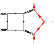
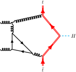
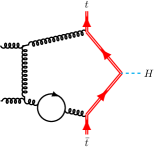
Figure 1: Examples of two-loop Feynman diagrams proportional to the number of light flavors $n_{f}$ contributing to leading-color two-loop scattering amplitudes for the process $gg\to t\bar{t}H$. The red double lines represent top quarks and the external cyan dashed line the Higgs boson. Light quarks are represented by black solid lines and gluons by black wavy lines.

The corresponding amplitudes and Feynman integrals depend on seven different kinematic scales, including the mass of the top quark (which also enters internal lines of Feynman diagrams) and the mass of the Higgs boson. Importantly, we note that these integrals also arise in the two-loop scattering amplitudes for processes such as $pp\to t\bar{t}Z$ and $e^{+}e^{-}\to t\bar{t}+2j$.

The set of Feynman integrals that we study is organized in terms of three integral families and contains a total of $127$ master integrals. We compute the integrals with the method of differential equations Kotikov:1990kg ; Kotikov:1991pm ; Bern:1993kr ; Remiddi:1997ny ; Gehrmann:1999as ; Henn:2013pwa , constructing a basis of master integrals that satisfies a set of differential equations in $\epsilon$-factorized form Henn:2013pwa . Having found such a basis, we uncover a novel feature of these Feynman integrals: their analytic description requires a nested square root function of the external kinematics. We then show that the differential equations can be expressed in terms of $152$ differential one-forms, of which we are able to express all but four in $\textrm{d}\log$ form. In such a compact form, our analytic differential equations clearly manifest the singularity structure of the integrals. We then explore the analytic properties of the master integrals by considering the iterated integrals which arise in solutions to the differential equations. Moreover, we solve the differential equations numerically using the generalized series expansion method Moriello:2019yhu as implemented in the DiffExp package Hidding:2020ytt . The required boundary values in the numerical solutions are obtained with the auxiliary mass flow method Liu:2017jxz ; Liu:2021wks ; Liu:2022tji as implemented in the AMFlow package Liu:2022chg . We provide in the ancillary files of this article a Mathematica implementation based on DiffExp that allows to solve the system of differential equations for points in the physical phase space.

The rest of this article is organized as follows. In section 2 we present the kinematic properties for the process studied and define a series of relevant Lorentz invariant functions. In section 3 we define the families of Feynman integrals that we study and describe the related master integrals. In section 4 we give details of our procedure to build the basis of master integrals that satisfy $\epsilon$-factorized differential equations and our method of determining the analytic form of said differential equations. In particular we discuss the determination of the corresponding “alphabet” of one-forms, and how we construct $\textrm{d}\log$ forms. In section 5 we consider the analytic structure of Feynman integrals, first discussing the alphabet in subsection 5.1 and then exploring the analytic properties of the corresponding function space in subsection 5.2. In section 6 we present numerical results based on generalized series expansions. We describe in subsection 6.3 the ancillary files provided with this article. Finally, in section 7 we give our conclusions and outlook. Appendices A, B, and C contain a detailed description of the integral bases we have constructed.

2 Scattering Kinematics and Notation

We consider the scattering process

$$q_{1}(p_{4})\,q_{2}(p_{5})\,\to\,t(p_{1})\,H(p_{2})\,\bar{t}(p_{3})\;,$$ (1)

where the initial pair of partons $(q_{1},q_{2})$ is either a gluon pair or a massless quark/anti-quark pair. For convenience we work in an all-incoming convention for the external momenta, such that momentum conservation is expressed as $\sum_{i=1}^{5}p_{i}=0$. The momenta fulfill the on-shell conditions

$$p_{1}^{2}=p_{3}^{2}=m_{t}^{2}\;,\qquad p_{2}^{2}=q^{2}\;,\qquad p_{4}^{2}=p_{5}^{2}=0\;,$$ (2)

where $m_{t}$ is the mass of the top quark and we have kept the momentum squared of the external massive boson in terms of the variable $q^{2}$. We write general kinematic invariants in terms of the scalar products $v_{ij}=2p_{i}\cdot p_{j}$, although for convenience we sometimes also use the Mandelstam variables $s_{ij}=(p_{i}+p_{j})^{2}$. The kinematic invariants can be expressed in terms of $7$ independent variables which we choose to be

$$\vec{s}=\{v_{12},v_{23},v_{34},v_{45},v_{15},m_{t}^{2},q^{2}\}\;,$$ (3)

together with the parity-odd invariant

$$\textrm{tr}_{5}=4i\epsilon_{\mu\nu\alpha\beta}\,p_{1}^{\mu}p_{2}^{\nu}p_{3}^{\alpha}p_{4}^{\beta}\;,$$ (4)

which is written in terms of the fully antisymmetric Levi-Civita symbol. In terms of these variables we can write all remaining scalar products as

$$\begin{split}v_{13}&=v_{45}-v_{12}-v_{23}-2m_{t}^{2}-q^{2}\;,\\ v_{14}&=v_{23}-v_{45}-v_{15}+q^{2}\;,\\ v_{24}&=v_{15}-v_{23}-v_{34}-q^{2}\;,\\ v_{25}&=v_{34}-v_{12}-v_{15}-q^{2}\;,\\ v_{35}&=v_{12}-v_{34}-v_{45}+q^{2}\;.\end{split}$$ (5)

When we consider the scattering process of equation (1), the physical phase space in the $\textrm{diag}(1,-1,-1,-1)$ Minkowski metric is a region in the space of Mandelstam variables that is specified by the following set of inequalities

$$\begin{split}m_{t}^{2}>0\ ,&\qquad q^{2}>0\ ,\\ v_{12}\geq 2\;m_{t}\;q\ ,\qquad v_{23}\geq 2\;m_{t}\;q\ ,&\qquad v_{34}\leq 0\ ,\qquad v_{15}\leq 0\ ,\\ v_{45}\geq(2m_{t}+q)^{2}\ ,\qquad\det G(p_{i},p_{j},p_{k})\geq 0\ ,&\qquad\det G(p_{1},p_{2},p_{3},p_{4})\leq 0\ ,\end{split}$$ (6)

where $q=\sqrt{q^{2}}$, the indices $i,j,k=1,\dots,5$, and we define the Gram matrix according to $G(q_{1},\dots,q_{n})_{ij}=q_{i}\cdot q_{j}$.

The integrals considered in this paper can be expressed in terms of a basis of special functions. One finds that these functions possess algebraic branch points on various surfaces. Some are given by the zero sets of the following Gram determinants

$$\Delta_{3}^{(1)} =-4\det G(p_{1},p_{2})=v_{12}^{2}-4m_{t}^{2}q^{2}\;,$$ (7)

$$\Delta_{3}^{(2)} =-4\det G(p_{2},p_{3})=v_{23}^{2}-4m_{t}^{2}q^{2}\;,$$ (8)

$$\Delta_{3}^{(3)} =-4\det G(p_{1},p_{2}+p_{3})=(q^{2}+v_{23}-v_{45})^{2}-4m_{t}^{2}v_{45}\;,$$ (9)

$$\Delta_{3}^{(4)} =-4\det G(p_{1}+p_{2},p_{3})=(q^{2}+v_{12}-v_{45})^{2}-4m_{t}^{2}v_{45}\;,$$ (10)

$$\Delta_{3}^{(5)} =-4\det G(p_{2},p_{3}+p_{4})=(q^{2}+v_{34}-v_{15})^{2}-4q^{2}(m_{t}^{2}+v_{34})\;,$$ (11)

$$\Delta_{5}\ \!\ =16\det G(p_{1},p_{2},p_{3},p_{4})=\textrm{tr}_{5}^{2}\;.$$ (12)

An important subtlety here is that one cannot identify $\textrm{tr}_{5}$ with $\sqrt{\Delta_{5}}$ as the first picks up a sign under parity, while the second is invariant. For simplicity, when handling the algebraic branch points, we will use $\sqrt{\Delta_{5}}$ instead of $\textrm{tr}_{5}$ throughout this paper, analogous to the conventions of Ref. Abreu:2021smk . Two further surfaces are given by the zero sets of of the functions

$$\mathcal{C}_{1} =q^{2}(q^{2}-4m_{t}^{2})\;,$$ (13)

$$\mathcal{C}_{2} =\Big{[}(q^{2}+v_{12})(q^{2}+v_{23})-q^{2}v_{45}\Big{]}\Big{[}(q^{2}+v_{12})(q^{2}+v_{23})-(q^{2}-4m_{t}^{2})v_{45}\Big{]}\;.$$ (14)

These functions can be associated to the maximal cut of one-loop Baikov polynomials Baikov:1996iu of the Feynman integrals in figure 2. Alternatively, they can be understood as modified Cayley determinants (see e.g. Ref. Abreu:2017mtm ).

(a) $\mathcal{C}_{1}$

(b) $\mathcal{C}_{2}$

Figure 2: One-loop Feynman integrals whose maximal cut Baikov polynomials are related to the $\mathcal{C}_{1}$ and $\mathcal{C}_{2}$ functions in equations (13) and (14). The red double lines represent massive internal and external lines (associated to top quarks in $t\bar{t}H$ production) while the dashed cyan line denotes an external off-shell line (associated to the Higgs boson in $t\bar{t}H$ production).

Three additional functions associated to leading singularities of the two-loop Feynman integrals shown in figure 3 will also be needed, and we define them according to

$$r_{1} =(v_{24}+v_{25})^{2}-4q^{2}v_{45}\;,$$ (15)

$$r_{2} =[q^{2}{}v_{35}+v_{23}(v_{35}+v_{45})]^{2}-4m_{t}^{2}{}v_{45}[v_{23}v_{25}-q^{2}{}(v_{15}+v_{35})]\;,$$ (16)

$$r_{3} =[q^{2}{}v_{14}+v_{12}(v_{14}+v_{45})]^{2}-4m_{t}^{2}{}v_{45}[v_{12}v_{24}-q^{2}{}(v_{14}+v_{34})]\;.$$ (17)

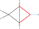
(a) $r_{1}$

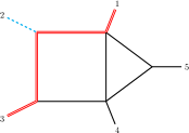
(b) $r_{2}$

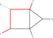
(c) $r_{3}$

Figure 3: Two-loop Feynman integrals with leading singularities associated to the $r_{1}$, $r_{2}$ and $r_{3}$ functions in equations (15)–(17). Diagram lines are as in figure 2.

In contrast to previous two-loop five-point master integral computations, the algebraic branch point structureis richer and involves nested square roots. Indeed, we will need to employ square roots of the quantities

$$N_{\pm}=q^{2}{}\left(N_{b}\pm\sqrt{N_{b}^{2}-N_{c}}\right)\;,$$ (18)

where

$$N_{b} =q^{2}{}\left[(v_{14}+v_{15})^{2}+(v_{34}+v_{35})^{2}\right]-2m_{t}^{2}{}(v_{24}+v_{25})^{2}\;,$$ (19)

$$N_{c} =\mathcal{C}_{1}(v_{12}-v_{23})^{2}(v_{24}+v_{25}+2v_{45})^{2}\;.$$ (20)

Note that there is a subtlety when considering square roots of $N_{\pm}$, as such roots are not algebraically independent from $\sqrt{\mathcal{C}_{1}}$. This follows as the $N_{\pm}$ fulfill

$$N_{+}\cdot N_{-}=(q^{2})^{2}~{}N_{c}\;.$$ (21)

In practice, throughout this manuscript, we choose to use this relation to define the symbol $\sqrt{N_{-}}$ in terms of the functions $\sqrt{N_{+}}$ and $\sqrt{\mathcal{C}_{1}}$ according to

$$\sqrt{N_{-}}\equiv\sqrt{\mathcal{C}_{1}}\,\frac{q^{2}(v_{12}-v_{23})(2q^{2}+v_{12}+v_{23}-2v_{45})}{\sqrt{N_{+}}}\;.$$ (22)

When considering algebraic branch points an important associated algebraic object is the Galois group. The Galois group is composed of all automorphisms of the field extension that is implicitly defined by the functions with such branch point singularities. In previous two-loop five-point Feynman integral computations, the automorphisms were given by transformations that flipped the signs of square roots in the algebraic functions. Naturally, the more complicated square root structure that we find by considering square roots of $N_{\pm}$ results in elements of the Galois group that are more intricate. Clearly, we have the standard sign flip associated to $\sqrt{N_{+}}$. However, we can see from equation (22) that the sign flip of $\sqrt{N_{-}}$ is achieved simultaneously with the sign flip of $\sqrt{\mathcal{C}_{1}}$. Further, we also have the automorphism

$$\alpha\quad:\quad\sqrt{N_{+}}\leftrightarrow\sqrt{N_{-}}\;,\quad\sqrt{N_{b}^{2}-N_{c}}\leftrightarrow-\sqrt{N_{b}^{2}-N_{c}}\;,$$ (23)

which simultaneously flips the sign of the “inner” square root, and swaps $\sqrt{N_{+}}$ with $\sqrt{N_{-}}$.

Finally, we also note that there is an interesting relevant kinematic map. Specifically, the set of integrals maps into itself under

$$\mathcal{Z}\quad:\quad p_{1}\leftrightarrow p_{3},\quad p_{4}\leftrightarrow p_{5}\;.$$ (24)

with $p_{2}$ left unchanged. Under this map our set of independent kinematic variables in equation (3) transforms as:

$$\{v_{12},v_{23},v_{34},v_{45},v_{15},m_{t}^{2},q^{2}\}\ \ \xrightarrow{\mathcal{Z}}\ \ \{v_{23},v_{12},v_{15},v_{45},v_{34},m_{t}^{2},q^{2}\}\;,$$ (25)

and then all functions defined above transform under $\mathcal{Z}$ according to

$$\Delta_{3}^{(1)}\leftrightarrow\Delta_{3}^{(2)}\;,\quad\Delta_{3}^{(3)}\leftrightarrow\Delta_{3}^{(4)}\;,\quad r_{2}\leftrightarrow r_{3}\;,\quad\sqrt{N_{-}}\rightarrow-\sqrt{N_{-}}\;,$$ (26)

while $\Delta_{3}^{(5)}$, $\Delta_{5}$, $\mathcal{C}_{1}$, $\mathcal{C}_{2}$, $r_{1}$ and $N_{+}$ remain invariant. Naturally, $\alpha$ and $\mathcal{Z}$ can be composed and we denote the composition as $[\alpha\circ\mathcal{Z}]$, which acts on a function $f$ as

$$[\alpha\circ\mathcal{Z}](f)\equiv\alpha\left(\mathcal{Z}(f)\right)\;.$$ (27)

3 Feynman Integral Families

There are six types of eleven-propagator Feynman integral families, namely one penta-box, two hexa-triangle, and three hepta-bubble families that contribute to the considered scattering amplitudes. We start by analyzing the number of master integrals that are associated to them. To find them we construct integration-by-parts (IBP) identities Tkachov:1981wb ; Chetyrkin:1981qh ; Laporta:2000dsw employing numerical evaluations, independently obtained with the software packages Kira Maierhofer:2017gsa ; Klappert:2020nbg and FIRE Smirnov:2019qkx . We find the following three main structures for the master integrals.

Penta-box integral family:

This family is associated to the propagator structure of the left diagram of figure 1. We find that this family has $111$ master integrals, including integrals with $3$ to $8$ propagators. We label this family of integrals as $T_{1}$, and we specify it below in detail. We notice that this integral family maps into itself under the $\mathcal{Z}$ transformation introduced in the previous section.

Hexa-triangle integral family:

This family is associated to the propagator structure of the central diagram in figure 1. We find that this family contains $46$ master integrals, of which $38$ are already contained in the $T_{1}$ family. This leaves $8$ distinct master integrals all of which are contained in a penta-bubble subsystem with $19$ master integrals. We label this subsystem as $\tilde{T}_{2}$ and specify it in detail below. The hexa-triangle integral family does not transform into itself under the $\mathcal{Z}$ map, therefore the $8$ distinct master integrals above map under $\mathcal{Z}$ to $8$ additional independent master integrals. We denote the corresponding integral family by $\mathcal{Z}(\tilde{T}_{2})$.

Hepta-bubble families:

These families are associated to the propagator structure of the right diagram in figure 1. They can be described in terms of the propagator structures that result from a massless bubble insertion in each of the internal massless lines of the corresponding one-loop diagram. We find that each of these families contain $19$ master integrals, all of which are contained in the $T_{1}$, $\tilde{T}_{2}$, and $\mathcal{Z}(\tilde{T}_{2})$ families described above.

In summary we have $127$ two-loop master integrals, decomposed into three distinct Feynman integral families that we denote as $T_{1}$ (with $111$ master integrals), $\tilde{T}_{2}$ (with $8$ independent master integrals), and $\mathcal{Z}(\tilde{T}_{2})$ (with $8$ independent master integrals). In the following subsections, as well as in Appendices A and B, we give further details about them. We notice that for completeness, in Appendix C we also provide details of our basis of one-loop master integrals for the propagator structure of the diagram shown in figure 7. In the following, we will refer to the one-loop topology as $T_{0}$.

3.1 The Penta-Box Family $T_{1}$

The $T_{1}$ family is an eleven-propagator Feynman integral family, where three propagators are introduced to make the family complete, such that all scalar products between loop momenta and external momenta can be expressed in terms of inverse propagators. It is defined according to

$$T_{1}[\vec{\nu}]=\int\frac{d^{d}\ell_{1}}{i\pi^{d/2}}\frac{d^{d}\ell_{2}}{i\pi^{d/2}}\frac{\rho_{9}^{-\nu_{9}}\rho_{10}^{-\nu_{10}}\rho_{11}^{-\nu_{11}}}{\rho_{1}^{\nu_{1}}\rho_{2}^{\nu_{2}}\rho_{3}^{\nu_{3}}\rho_{4}^{\nu_{4}}\rho_{5}^{\nu_{5}}\rho_{6}^{\nu_{6}}\rho_{7}^{\nu_{7}}\rho_{8}^{\nu_{8}}}\;,$$ (28)

where $\vec{\nu}=(\nu_{1},\cdots,\nu_{11})$ is a vector of integers (the propagator powers) and $\nu_{i}\leq 0$ for $i=9,10$ and $11$. We work in dimensional regularization with $d=4-2\epsilon$ and the inverse propagators are defined according to

$$\rho_{1}=\ell_{1}^{2}\;, \rho_{2}=(\ell_{1}+p_{1})^{2}-m_{t}^{2}\;, \rho_{3}=(\ell_{1}+p_{12})^{2}-m_{t}^{2}\;,$$

$$\rho_{4}=(\ell_{1}+p_{123})^{2}\;, \rho_{5}=(\ell_{1}+\ell_{2})^{2}\;, \rho_{6}=\ell_{2}^{2}\;,$$ (29)

$$\rho_{7}=(\ell_{2}+p_{5})^{2}\;, \rho_{8}=(\ell_{2}+p_{45})^{2}\;,$$

where $p_{i\cdots j}=p_{i}+\cdots+p_{j}$. These propagators correspond to the diagram shown in figure 4, to which we add the three irreducible scalar products

Figure 4: The propagator structure associated to the $T_{1}$ integral family, with the routing of loop momenta $\ell_{i}$ ($i=1,2$) chosen as in equation (29). The red double lines represent massive propagators or external on-shell momenta (with mass $m_{t}$), the black solid lines represent massless propagators or external on-shell momenta, and the cyan dashed line represents an external off-shell momentum. The integers labeling the external lines refer to the corresponding momenta $p_{i}$ ($i=1,\cdots,5$) as defined in section 2, while the blue inner integers correspond to the inverse propagators $\rho_{j}$ ($j=1,\cdots,8$) as defined in equation (29).

$$\rho_{9}=(\ell_{1}-p_{5})^{2}\;, \rho_{10}=(\ell_{2}-p_{12})^{2}-m_{t}^{2}\;, \rho_{11}=(\ell_{2}-p_{1})^{2}-m_{t}^{2}\;.$$ (30)

The integral family $T_{1}$ defines a vector space of integrals. Each element of this vector space can be systematically expressed in terms of basis elements with the help of IBP identities. As described above, the dimension of this vector space is $\textrm{dim}\left(T_{1}\right)=111$. There is a lot of freedom in the choice of a basis of integrals, the so-called master integrals, and in section 4 we describe how we construct a basis that satisfies a set of differential equations in $\epsilon$-factorized form. In such way we make explicit the singularity structure of all master integrals. We notice that $50$ master integrals of $T_{1}$ have never been studied in the literature, with the rest being one-loop squared integrals, $3$-propagator integrals, integrals with all massless propagators, or integrals studied in Ref. Badger:2022hno . In Appendix A we include the definition of all $111$ integrals in our basis.

3.2 The Penta-Bubble Family $\tilde{T}_{2}$

The penta-bubble family $\tilde{T}_{2}$ is defined according to:

$$\tilde{T}_{2}[\vec{\nu}]=\int\frac{d^{d}\ell_{1}}{i\pi^{d/2}}\frac{d^{d}\ell_{2}}{i\pi^{d/2}}\frac{\rho_{7}^{-\nu_{7}}\rho_{8}^{-\nu_{8}}\rho_{9}^{-\nu_{9}}\rho_{10}^{-\nu_{10}}\rho_{11}^{-\nu_{11}}}{\rho_{1}^{\nu_{1}}\rho_{2}^{\nu_{2}}\rho_{3}^{\nu_{3}}\rho_{4}^{\nu_{4}}\rho_{5}^{\nu_{5}}\rho_{6}^{\nu_{6}}}\;,$$ (31)

where $\nu_{i}\leq 0$ if $i=7,\ldots,11$. The inverse propagators are defined according to

$$\rho_{1}=\ell_{1}^{2}\;, \rho_{2}=(\ell_{1}+p_{5})^{2}\;, \rho_{3}=(\ell_{1}+p_{15})^{2}-m_{t}^{2}\;,$$

$$\rho_{4}=(\ell_{1}+p_{125})^{2}-m_{t}^{2}\;, \rho_{5}=(\ell_{1}+\ell_{2}-p_{4})^{2}\;, \rho_{6}=\ell_{2}^{2}\;,$$ (32)

which correspond to the diagram shown in figure 5. We add the following five irreducible scalar products to complete the family

$$\rho_{7}=(\ell_{1}-p_{3})^{2}\;, \rho_{8}=(\ell_{2}-p_{1})^{2}\;, \rho_{9}=(\ell_{2}-p_{2})^{2}\;,$$

$$\rho_{10}=(\ell_{2}-p_{3})^{2}\;, \rho_{11}=(\ell_{2}-p_{4})^{2}\;.$$ (33)

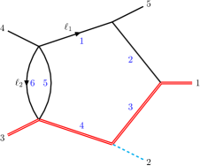
Figure 5: The propagator structure associated to the $\tilde{T}_{2}$ integral family, with the routing of loop momenta $\ell_{i}$ ($i=1,2$) chosen in equation (32). See caption of figure 4 for details on the notation.

The integral family $\tilde{T}_{2}$ defines a vector space with $\textrm{dim}(\tilde{T}_{2})=19$. As described above, only $8$ of those integrals are not included in the $T_{1}$ family, and $4$ of them have never been studied in the literature. Considering also the $\mathcal{Z}(\tilde{T}_{2})$ family introduces $16$ more master integrals in our analysis. In Appendix B we include the definition of all $\tilde{T}_{2}$ master integrals not included in $T_{1}$.

4 Differential Equations in $\epsilon$-Factorized Form

The method of differential equations Kotikov:1990kg ; Kotikov:1991pm ; Bern:1993kr ; Remiddi:1997ny ; Gehrmann:1999as ; Henn:2013pwa has become one of the most used approaches for computing master integrals, especially in the case of integrals involving multiple scales. In practice, it turns out that obtaining the analytic form of the differential equation can be challenging. Nevertheless, a major simplification is achieved when the master integrals are chosen to satisfy a differential equation in $\epsilon$-factorized form  Henn:2013pwa . Despite great theoretical progress (see e.g. Lee:2014ioa ; Prausa:2017ltv ; Gituliar:2017vzm ; Dlapa:2020cwj ; Henn:2020lye ; Lee:2020zfb ; Dlapa:2021qsl ; Chen:2022lzr ; Dlapa:2022wdu ; Gorges:2023zgv ), finding such sets of master integrals for multi-scale problems remains a major problem. In this section we give details of our approach to construct a basis of master integrals satisfying $\epsilon$-factorized differential equations, which builds upon the numerical approaches presented in Abreu:2020jxa ; Abreu:2021smk ; Tschernow:2022kit .

Let us denote a basis of master integrals as $\vec{J}$ for a family of Feynman integrals $T$. The integrals $\vec{J}$ are functions of the kinematic invariants $\vec{s}$ and the dimensional regulator $\epsilon=(4-d)/2$. A basis of master integrals satisfies a set of first-order partial differential equations

$$\frac{\partial\vec{J}}{\partial s_{i}}=B_{i}(\vec{s},\epsilon)~{}\vec{J}\;,$$ (34)

where the $B_{i}(\vec{s},\epsilon)$ are $N\times N$ matrices, with $N=\textrm{dim}(T)$ and entries which are rational functions of $\epsilon$. If the choice of basis $\vec{J}$ does not include algebraic functions of $\vec{s}$, such as square roots, then the differential equation matrices $B_{i}(\vec{s},\epsilon)$ are also rational functions of $\vec{s}$. Differential equations of the form (34) are neither easy to construct, nor easy to solve. To remedy these difficulties, we change to a basis of master integrals $\vec{I}$ via $\vec{J}=U\vec{I}$, which satisfy differential equations of the form

$$\frac{\partial\vec{I}}{\partial s_{i}}=\epsilon\,A_{i}(\vec{s}\!\;)\vec{I}\;.$$ (35)

The differential equation matrices $A_{i}(\vec{s}\,)$ are related to those of the original differential equation by

$$\epsilon\,A_{i}(\vec{s}\!\;)=U^{-1}B_{i}(\vec{s},\epsilon)U-U^{-1}\frac{\partial U}{\partial s_{i}}\;.$$ (36)

The key feature of equation (35) is that it is in “$\epsilon$-factorized” form. In general, finding a basis of master integrals $\vec{I}$ that satisfies such differential equations is a non-trivial task. We describe our approach in the next section. In practice, we find that we are able to achieve such an $\epsilon$-factorized form with a change of basis matrix $U$ that is algebraic in the kinematic invariants and rational in $\epsilon$. Hence, the $A_{i}(\vec{s}\,)$ are algebraic in the kinematics invariants.

In practice, it is useful to unify the $7$ differential equations into a single one using the language of differential forms. In such a language, we write that

$$\mathrm{d}\vec{I}=\epsilon\sum_{\alpha=1}^{\kappa}M_{\alpha}\,\omega_{\alpha}\vec{I}\;,$$ (37)

where we express the differential equation in terms of a set of $\kappa$ linearly independent differential one-forms $\omega_{\alpha}$. We call such a one-form a “letter”, and the full collection of all $\kappa$ letters, the “alphabet”. The coefficient matrices $M_{\alpha}$ are $N\times N$ matrices with rational number entries.

In the following subsections we describe the procedure to construct our basis of master integrals $\vec{I}$ that satisfy equation 37, alongside the associated set of letters $\omega_{\alpha}$, and rational number matrices $M_{\alpha}$.

4.1 Construction of Master Integral Basis

In order to construct a basis of master integrals that satisfy an $\epsilon$-factorized differential equation, we follow the strategies employed in Refs. Abreu:2020jxa ; Abreu:2021smk ; Tschernow:2022kit . Starting from a choice of master integrals, for example by following the Laporta algorithm Laporta:2000dsw , we construct the differential equations (34) on a fixed kinematic point while keeping the full $\epsilon$ dependence. This allows to explore the analytic form of the differential equations as a function of the dimensional regulator for multiple choices of integral bases in an efficient way. We employ the Kira program Maierhofer:2017gsa ; Klappert:2020nbg for these reductions using finite fields $\mathbb{F}_{p}$ where $p$ is a large prime number vonManteuffel:2014ixa ; Peraro:2016wsq . We then follow a number of approaches to refine the basis choice, building on experience from the literature and using a variety of techniques that we summarize here.

As a first step, we search for a collection of master integrals where the differential equations are linear in $\epsilon$. That is, we search for a basis such that the matrix $B_{i}(\vec{s},\epsilon)$ in equation (34) takes the form

$$B_{i}(\vec{s},\epsilon)=B_{i}^{(0)}(\vec{s}\!\;)+\epsilon B_{i}^{(1)}(\vec{s}\!\;)\;,$$ (38)

We proceed in a bottom-up fashion, starting with master integrals with the fewest number of propagators. For integrals with a low number of propagators, we search through a collection of basis integrals with raised propagator powers, until the differential equations take a form that is linear in $\epsilon$. Often, such bases must be normalized by various $\epsilon$-dependent functions, which we read from the differential equations evaluated on a numerical kinematic point. A number of such basis choices can be interpreted as dimension shift relations Tarasov:1996br ; Lee:2009dh of subloops, such as considering tadpole and bubble subloops into $2-2\epsilon$ dimensions. This procedure gives rise to a large number of integrals in our basis, for example those given in equations (117), (168), (185) and (203). For many integrals with a higher number of propagators, we instead consider simple tensor insertions in order to arrive at a differential equation that is linear in $\epsilon$.

From the refined starting point of equation (38), we apply a number of techniques to obtain $\epsilon$-factorized differential equations. For integrals with box or pentagon subloops, we follow techniques introduced elsewhere in the literature Abreu:2020jxa ; Abreu:2021smk ; Abreu:2023rco . Some examples were constructed by considering a four-dimensional $\textrm{d}\log$-form integrand analysis (see e.g. Henn:2020lye ). Others make use of numerators built from $\epsilon$-dimensional scalar products Abreu:2018rcw

$$\mu_{ij}=\ell_{i}^{[d-4]}\cdot\ell_{j}^{[d-4]}\;,\qquad i,j=1,2\;,$$ (39)

where we write the loop momenta as $\ell_{i}=(\ell_{i}^{[4]},\ell_{i}^{[d-4]})$, i.e. decomposing them in terms of their 4- and $(d-4)$-dimensional parts. Examples of integrands obtained through this procedure for $T_{1}$ can be found in equations (190), (202) and (222), and for $\tilde{T}_{2}$ in equations (227), (231) and (232).

For many other integrals, it was fruitful to employ an approach based on the structure of the $\epsilon\to 0$ limit of the differential equation matrix. One advantage of the linear-in-$\epsilon$ form is that a change of basis matrix that satisfies

$$\frac{\partial}{\partial s_{i}}U=B^{(0)}_{i}(\vec{s}\,)U\;,$$ (40)

will result in a differential equation in $\epsilon$-factorized form. This allows us to use techniques based on the Magnus exponential Argeri:2014qva , which we combine with analytic reconstruction techniques. In practice, we work sector by sector, or equivalently block by block of $B^{(0)}_{i}$, and make a series of partial basis changes to sequentially improve the basis. In most sectors we find that the $B^{(0)}_{i}$ are triangular, and proceed in two stages. In the first stage, we restrict our analysis of equation (40) to diagonal entries, which reduces equation (40) to a collection of $1\times 1$ systems. In practice, we find that these systems take the form

$$\frac{\partial}{\partial s_{i}}u=b_{i}u\;,\qquad\text{where}\qquad b_{i}=\frac{\partial}{\partial s_{i}}\log(\tilde{b})\;,$$ (41)

where $u$ is a diagonal entry of $U$ and $b_{i}$ are diagonal entries of $B_{i}^{(0)}$. By analytically reconstructing the $b_{i}$ and integrating, we find an associated normalization of the corresponding integral. We note that it may be the case that the $b_{i}$ are rational, while $\tilde{b}$ is algebraic. In practice, we find that this procedure is often easier to automate than a leading singularity calculation in momentum space. In the second stage, we can assume that the relevant block of each $B^{(0)}_{i}$ is strictly lower triangular. As an example, let us assume that the relevant block is $2\times 2$. Larger cases can be similarly handled. One then has that

$$\frac{\partial}{\partial s_{i}}U=\left(\begin{array}[]{cc}0&0\\ b_{10,i}&0\\ \end{array}\right)U\;,\qquad\text{where}\qquad b_{10,i}=\frac{\partial}{\partial s_{i}}\tilde{b}_{10}\;,$$ (42)

and in practice we find that $\tilde{b}_{10}$ is an algebraic function of the kinematics. This differential equation is then solved by

$$U=\left(\begin{array}[]{cc}1&0\\ \tilde{b}_{10}&1\\ \end{array}\right),$$ (43)

which can be read as an instruction to redefine the second integral in the block by subtracting the first with a factor of $\tilde{b}_{10}$. When encountering situations like this, we analytically reconstruct $b_{10}$ to find the associated basis change. Example of integrals obtained through this procedure are in equations (205), (209) and (219) for $T_{1}$.

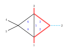
Figure 6: The “kite₇” sector with seven master integrals. When studying the differential equations for these integrals using Magnus exponential techniques, the associated matrix is not triangular. The result of the Magnus exponential for this sector introduces the nested square roots $\sqrt{N_{\pm}}$ (see section 2).

A particular five-propagator sector, displayed in figure 6, involves $7$ master integrals and requires special attention, as the relevant block structure of $B_{i}^{(0)}$ is not triangular. We refer to this sector as the kite₇. Four such integrals arise in a lower triangular block and so an $\epsilon$-factorizing basis can be constructed with the procedures described before. However, it was necessary to study a non-triangular $3\times 3$ block. Here, we again start by focusing on the diagonal entries, leading to normalizations for the involved integrals which eliminate the diagonal elements of the $B_{i}^{(0)}$. This leads to studying the differential equation for the integrals with the numerators

$$\begin{split}\widetilde{\mathcal{N}}_{64}^{(1)}&=\epsilon^{3}\sqrt{q^{2}}\sqrt[4]{N_{b}^{2}-N_{c}}\left(\frac{1}{\rho_{3}}-\frac{1}{\rho_{2}}\right)\;,\\ \widetilde{\mathcal{N}}_{65}^{(1)}&=\epsilon^{3}\sqrt{q^{2}-4m_{t}^{2}}\sqrt[4]{N_{b}^{2}-N_{c}}\left(\frac{1}{\rho_{3}}+\frac{1}{\rho_{2}}\right)\;,\\ \widetilde{\mathcal{N}}_{66}^{(1)}&=\epsilon^{2}\frac{m_{t}^{2}v_{45}(q^{2}+v_{12})(q^{2}+v_{23})}{2q^{2}+v_{12}+v_{23}}\left(\frac{1}{\rho_{2}\rho_{6}}+\frac{1}{\rho_{3}\rho_{8}}\right)\;.\end{split}$$ (44)

where the tilded notation highlights that this is an intermediate step in the production of the final $\epsilon$-factorized basis. The corresponding differential equations take the form

$$\frac{\partial}{\partial s_{i}}\begin{pmatrix}\widetilde{I}_{64}\\ \widetilde{I}_{65}\\ \widetilde{I}_{66}\end{pmatrix}=\begin{pmatrix}0&a_{i}&0\\ a_{i}&0&0\\ b_{i}&c_{i}&0\end{pmatrix}\begin{pmatrix}\widetilde{I}_{64}\\ \widetilde{I}_{65}\\ \widetilde{I}_{66}\end{pmatrix}+\mathcal{O}(\epsilon),\qquad\text{where}\qquad a_{i}=\frac{1}{4}\frac{\partial}{\partial s_{i}}\log(\tilde{a})\;,$$ (45)

and $a_{i},b_{i},c_{i}$ and $\tilde{a}$ are algebraic functions of the kinematics. We then work to construct a change of basis which renders the matrix lower triangular, and therefore amenable to the previous techniques. This leads us to focus only on the upper $2\times 2$ block. To remove this block, we solve the associated differential equation for the change of basis matrix of equation (40) using the Magnus exponential. As the two off-diagonal entries involve the same functions $a_{i}$, the Magnus exponential truncates at its first order. Nevertheless, the factor of $\frac{1}{4}$ in equation (45) leads to a complicated algebraic procedure which eventually results in removing the quartic roots in equation (44), but introducing the nested roots $\sqrt{N_{\pm}}$ of equation (18). After this step, the resulting block is now lower triangular, and can be handled as discussed above. To apply this procedure in practice, we reconstruct the analytic form of the $a_{i},b_{i}$ and $c_{i}$ from numerical samples. The integrals obtained through this procedure are presented in equations (166), (167) and (168).

Altogether, using this suite of approaches, we were able to construct a basis of master integrals that satisfy a set of differential equations in $\epsilon$-factorized form. We present the full set of basis integrals in the appendices A and B for the $T_{1}$ and $\tilde{T}_{2}$ families respectively.

4.2 Analytic Reconstruction of the Differential Equations

Given that the bases of integrals obtained in the last section satisfy a set of differential equations in $\epsilon$-factorized form, we are now in a position to compute the analytic form of the differential equations. We follow the general procedure of Ref. Abreu:2020jxa . We begin by computing $\kappa$, the number of linearly independent letters $\omega_{\alpha}$ that arise in equation (37). As described in Ref. Abreu:2020jxa , this can be computed from repeated numerical evaluations of the differential equations. In practice, we find that the number of linearly independent letters, or the dimension of the alphabet, is

$$\kappa=152\;.$$ (46)

Furthermore, we observe that by itself the $T_{1}$ family contains all $152$ independent letters, and that the families $\tilde{T}_{2}$, $\mathcal{Z}$($\tilde{T}_{2}$) and $T_{0}$ can be expressed in terms of a subset of the same letters.

Next, we focus on reconstructing a basis of letters, onto which we will later fit the full differential equations. This approach avoids reconstructing the functional form of each entry of the differential equations with numerical evaluations, which can become computationally prohibitive. Following Refs. Abreu:2018rcw ; Abreu:2018aqd ; Abreu:2020jxa , we choose a basis of linearly independent letters by prioritizing entries of the differential equation that lie on the block-diagonal. In practice, we find that $80$ of the letters can be obtained from maximal-cut, $70$ from next-to-maximal-cut, and $2$ are found on next-to-next-to-maximal-cut differential equations.

Our approach to reconstructing the basis of letters is based upon expectations for their analytic form. Given that we have found a basis with an $\epsilon$-factorized differential equation using only algebraic functions, we naively expect that the letters can be expressed in $\textrm{d}\log$ form, i.e.

$$\omega_{\alpha}=\textrm{d}\log(W_{\alpha})\;.$$ (47)

which gives a strong constraint on their analytic structure. We will return to the validity of this assumption later. Further constraints on the analytic structure of the letters follow from their properties under Galois transformations. We start with letters that are independent of the square roots and therefore have trivial Galois transformations. We call these even letters. If a given letter $\omega_{\alpha}$ is even

$$\omega_{\alpha}=\sum_{i}\omega_{\alpha,i}\;\textrm{d}s_{i}\;,$$ (48)

it is clear that the $\omega_{\alpha,i}$ are rational functions. Given the $\textrm{d}\log$-form expectation, we should have that

$$\omega_{\alpha,i}=\frac{\frac{\partial}{\partial s_{i}}W_{\alpha}}{W_{\alpha}}\;.$$ (49)

Thus, irreducible polynomial factors of denominators of the $\omega_{\alpha,i}$ are natural candidates for even letters. We therefore proceed to compute the rational functions $\omega_{\alpha,i}$ through functional reconstruction techniques (see e.g. Refs. Peraro:2016wsq ; Klappert:2019emp ), and take the irreducible factors as letter candidates. In practice, this procedure allowed us to compute a set of $33$ $W_{\alpha}$, which generate the full subspace of even letters $\omega_{\alpha}$.

Next, we consider letters with non-trivial properties under Galois transformations. We first consider those which do not depend on the nested roots $\sqrt{N_{\pm}}$ but may depend on any other square root. In contrast to the even letters, finding the corresponding $W_{\alpha}$ of equation (47) is considerably more challenging and we dedicate most of the rest of this section to their determination. Due to the way in which the algebraic functions are introduced into our choice of basis, the corresponding entries of the differential equation matrices (and therefore letters) all pick up a sign under sign-flip Galois transformations. We refer to these as odd letters. An important feature observed in all odd letters in two-loop five-point computations to date is that the possible denominator factors of the associated differential form correspond to the even letters. Given these two features, denoting the relevant square root as $\sqrt{R}$, we are motivated to consider an initial ansatz for odd $\omega_{\alpha}$ of the form

$$\omega_{\alpha}=\frac{1}{\sqrt{R}}\frac{N_{\alpha}}{\prod_{\beta}(W_{\beta}^{\text{even}})^{q_{\alpha\beta}}}\;,$$ (50)

where $N_{\alpha}$ is a polynomially valued differential form and the $q_{\alpha\beta}$ take values in $\{0,1\}$ and therefore select which even letters arise in the denominators. In order to determine these exponents, given that the set of even letters has already been determined, we apply univariate reconstruction approaches Abreu:2018zmy to each of the individual $\omega_{\alpha,i}$, and take the lowest common multiple of the set in $i$ of all denominators in the $\omega_{\alpha,i}$.

Naturally, for each such letter, two steps remain: first we must determine the numerators $N_{\alpha}$ and then we must perform the integration to rewrite $\omega_{\alpha}$ as a $\textrm{d}\log$ form. In practice each of these steps are computationally and theoretically demanding. Instead, we perform both operations together, using an ansatz approach. Specifically, we build ansätze for the arguments of our $\textrm{d}\log$ forms $W_{\beta}$ using the function

$$\Omega_{1}(w,R)=\frac{w-\sqrt{R}}{w+\sqrt{R}}\;.$$ (51)

For the purposes of the ansatz procedure, we will consider $w$ as an unknown rational function of the Mandelstam invariants. In order to constrain $w$, let us consider the structure of a $\textrm{d}\log$ form arising from $\Omega_{1}$,

$$\textrm{d}\log(\Omega_{1}(w,R))=\frac{-w(\mathrm{d}R)+2R(\mathrm{d}w)}{\sqrt{R}(w^{2}-R)}\;.$$ (52)

Here, we see that the denominator of the $\textrm{d}\log$ form is given by $w^{2}-R$. If we write $w=w_{N}/w_{D}$, where $w_{X}$ (with $X$ either $N$ or $D$) are polynomials and compare the denominators of equation (52) and equation (50) we find

$$w_{N}^{2}-Rw_{D}^{2}\sim\prod_{\beta}(W_{\beta}^{\text{even}})^{q_{\alpha\beta}}\;,$$ (53)

where we use $\sim$ to state that the left-hand side and right-hand side are (polynomially) proportional. We therefore reduce the problem to finding polynomials $w_{N}$ and $w_{D}$ that satisfy equation (53). This constraint is similar to that proposed in Ref. Heller:2019gkq , however here the product of even letters is known a priori.

In order to solve equation (53), we use two methods. First, we consider an ansatz for $w_{N}$ and $w_{D}$ where they are taken to be as multivariate polynomials with rational numbers as coefficients. That is, we write

$$w_{X}=\sum_{|\vec{\gamma}|=\text{deg}(w_{X})}\tau_{{X},\vec{\gamma}}\left(\prod_{i=1}^{7}s_{i}^{\gamma_{i}}\right)\;,$$ (54)

where the $\tau_{{X},\vec{\gamma}}$ are unknown rational numbers, $|\vec{\gamma}|=\sum_{i}\gamma_{i}$ and $\text{deg}(f)$ is the total degree of the polynomial $f$. The sum in equation (54) is over all exponents $\vec{\gamma}$ that have the same degree as the $w_{X}$. By equation (53), the degrees of $w_{N}$ and $w_{D}$ are constrained such that their difference is the mass dimension of $w$. The degree of $w_{D}$ is therefore another unknown, and in practice we vary this in the ansatz procedure. With this parametrization, we can rewrite equation (53) as

$$w_{N}^{2}-Rw_{D}^{2}\quad\text{mod}\quad\prod_{\beta}(W_{\beta}^{\text{even}})^{q_{\alpha\beta}}=0\;.$$ (55)

The modulo operation can then be implemented with polynomial reduction techniques that are commonly implemented in computer algebra systems (CAS). In this way, equation (55) becomes a quadratic set of constraints that the $\tau_{X,\vec{\gamma}}$ must satisfy.

Let us consider how to solve equation (55) given the multivariate polynomial ansätze for $w_{N}$ and $w_{D}$. First, note that any rescaling of equation (54) of the form

$$(\tau_{N,\vec{\gamma}},\tau_{D,\vec{\gamma}})\rightarrow(\lambda\tau_{N,\vec{\gamma}},\lambda\tau_{D,\vec{\gamma}})\;,$$ (56)

for any non-zero $\lambda$, will leave $w$ invariant. This implies that solutions to equation (55) are not unique and come in families. This non-uniqueness can be avoided in any case where we know that some $\tau_{X,\vec{\gamma}}$ is non-zero as we can use the rescaling to set it to 1. For example, if we consider a case where the degree of $w_{D}$ is 0, i.e. $w$ is simply a polynomial, then it is natural to use the rescaling to set $w_{D}=1$. In practice, we find that this results in a quadratic system of equations for the $(\tau_{N,\vec{\gamma}},\tau_{D,\vec{\gamma}})$ that have a finite number of solutions. Algorithms for enumerating the solutions of such systems are commonly implemented in computer algebra systems. In practice, we find it helpful to further organize the system by (repeatedly) solving all equations of the form $x^{2}=0$. Nevertheless, if $w_{D}$ has non-zero degree, then it is a priori unclear which term in $w_{D}$ is non-zero and we must walk through all possibilities before we find a term which we can choose to have unit coefficient.

In practice, as the number of terms in a multivariate polynomial grows rapidly as a function of the polynomial degree, the enumeration through all possible non-zero terms can be computationally prohibitive. To address this problem, we consider a second approach. Here, we single out one of the Mandelstam invariants, denoting it as $s_{i}$, which is chosen in an ad-hoc manner. We then consider an ansatz for $w_{N}$ and $w_{D}$ where they are univariate rational function in the variable $s_{i}$, that is

$$w_{X}=\sum_{k=0}^{\text{deg}(w_{X})}\tau_{X,k}^{(\hat{s}_{i})}(s_{i})^{k}\;,$$ (57)

where the $\tau_{X,k}^{(\hat{s}_{i})}$ are rational functions of all invariants other than $s_{i}$. Here, we fix the degrees in $s_{i}$ of the $w_{X}$ to be the largest possible, without the left hand side of equation (53) having greater degree in $s_{i}$ than the right hand side of equation (53). With the ansatz in equation (57), we again consider equation (55), this time implementing the modulo operation using polynomial reduction with respect to only $s_{i}$. Once again, this leads to a quadratic system of equations that the $\tau_{X,k}^{(\hat{s}_{i})}$ solve. While one must also determine which $\tau_{X,k}^{(\hat{s}_{i})}$ is non-zero by enumeration, the number of terms in a univariate rational function is much smaller, and is hence more tractable. Nevertheless, the $\tau_{X,k}^{(\hat{s}_{i})}$ are rational functions, and solving for them is a non-trivial exercise which we confront using an in-house implementation of “companion matrix” techniques (see, for example, Ref. Jiang:2017phk ; cox2006using ). In practice, we find this univariate ansatz method is able to handle the suite of complicated cases we study in this work.

In summary, with this ansatz procedure, we are able to construct a collection of $\textrm{d}\log$ forms whose denominators must correspond to the provided differential form. We then use these even $\textrm{d}\log$ forms as an ansatz for the odd forms (under a single square root) of the differential equations. The validity of this ansatz is confirmed by a numerical fitting procedure. Importantly, we did not directly reconstruct the numerator of equation (50). Instead, we have implicitly constructed it by using the expectation that equation (50) corresponds to a $\textrm{d}\log$ form.

Beyond the letters which are odd under a single Galois transformation, there are also letters which are odd under two such transformations. To handle these cases, we follow an analogous approach to the one just described. Specifically, denoting the two corresponding roots as $\sqrt{R_{1}}$ and $\sqrt{R_{2}}$, we start from an ansatz for the argument of the $\textrm{d}\log$ form using the function

$$\Omega_{2}(w,R_{1},R_{2})=\frac{w-\sqrt{R_{1}}\sqrt{R_{2}}}{w+\sqrt{R_{1}}\sqrt{R_{2}}}\;,$$ (58)

where $w$ is again an unknown rational function. Finally, it is sometimes useful to consider an ansatz for the argument of the $\textrm{d}\log$ form using the function

$$\tilde{\Omega}(w_{0},w_{1}\sqrt{R_{1}},\sqrt{R_{2}})=\frac{(w_{0}+w_{1}\sqrt{R_{1}}+\sqrt{R_{2}})(w_{0}-w_{1}\sqrt{R_{1}}-\sqrt{R_{2}})}{(w_{0}-w_{1}\sqrt{R_{1}}+\sqrt{R_{2}})(w_{0}+w_{1}\sqrt{R_{1}}-\sqrt{R_{2}})}\;.$$ (59)

Here, $w_{0}$ and $w_{1}$ are unknown rational functions. Such forms of letters have been previously found in multi-scale two-loop five-point amplitude calculations Abreu:2020jxa ; Abreu:2021smk ; Badger:2022hno . Indeed, early iterations of the multivariate rational function ansatz procedure were used to determine the most complicated letters in Abreu:2021smk . In practice, this can be a fruitful approach to simplify the result as the mass dimension of the unknown functions in equation (59) is lower than those of equation (58).

We now return to the collection of letters that depend on the nested square roots $\sqrt{N_{\pm}}$. In these cases, we construct the full differential form using functional reconstruction techniques. In practice, this was the most computationally demanding reconstruction procedure. In all but four cases, these were then integrated to $\textrm{d}\log$ forms using ad-hoc techniques. The remaining four letters proved resilient to being cast in $\textrm{d}\log$ form, and we suggest that it is indeed impossible to do so. Given that the differential equation is in $\epsilon$-factorized form, and the change of basis matrix is only algebraic, this feature is perhaps surprising. Nevertheless, this is not the only known example of such a case VitaPrivateCommunication . In practice, we suggest that this feature is due to the algebraic structure of $\sqrt{N_{\pm}}$, which can be shown to correspond to a curve of genus $1$.

Finally, with this complete alphabet in hand, we determine the rational number matrices $M_{\alpha}$ of equation (37) using the procedure described in Ref. Abreu:2020jxa . Specifically, we sample the differential equation $\kappa$ times, and use this information to fit the differential equations onto the basis of letters, yielding the $M_{\alpha}$ and therefore the analytic form of equation (37). Note that for this procedure to work it is enough to know the partial derivatives of the letters $\omega_{\alpha}$ for which we could not find a $\textrm{d}\log$ form. We provide the results of this procedure in the next section, as well as in a series of ancillary files that we describe in section 6.3.

5 Analytic Structure of the Feynman Integrals

Given our analytic determination of an $\epsilon$-factorized differential equation for the Feynman integrals studied in this paper, we are now in the position to investigate the analytic structure of these integrals. In the following we first discuss the organization of the letters in the alphabet of the differential equation and afterwards the analytic structures of the solution of the Feynman integrals.

5.1 The Alphabet

In section 4, we described a procedure to determine a set of $148$ out of $152$ letters as $\textrm{d}\log$ forms and that can be used to express the differential equation matrices. Here we present the results of that procedure, that is the analytic forms for the letters. Almost all letters are so-called $\textrm{d}\log$-forms, and take the form

$$\omega_{\alpha}=\textrm{d}\log(W_{\alpha})\;,$$ (60)

for some expression $W_{\alpha}$ that is algebraic in the Mandelstam invariants, depending on a limited series of square roots defined in section 2. In a slight abuse of language, in situations where there is no ambiguity, for letters $\omega_{\alpha}$ that are in $\mathrm{d}\log$ form we will also call the associated $W_{\alpha}$ a letter. As a first organizational criteria for the alphabet, we note that a number of letters do not arise in iterated integral solutions before $\mathcal{O}(\epsilon^{5})$ and hence do not contribute to the NNLO QCD corrections to associated physical observables. We will return to this discussion in section 5.2. We denote the set of letters that do contribute as relevant letters and consider these first.

The first set of relevant letters that we consider are those that appear in the first entry of iterated integral solutions,

$$\{W_{1},\ldots,W_{7}\}\!=\!\left\{\!s_{12}-m_{t}^{2}{},s_{23}-m_{t}^{2}{},s_{34}-m_{t}^{2}{},s_{15}-m_{t}^{2}{},v_{45},m_{t}^{2}{},\frac{q^{2}\!+\!\sqrt{\mathcal{C}_{1}}}{q^{2}\!-\!\sqrt{\mathcal{C}_{1}}}\right\}\;.$$ (61)

Note that one such letter is algebraic, and is odd under the Galois transformation associated to $\sqrt{\mathcal{C}_{1}}$. This letter can readily be associated to the one-loop bubble shown in figure 2(a).

Beyond the first entries, the letters can be organized in terms of the square roots that arise. The first class does not depend on any square root and are denoted by even letters. There are $33$ such relevant letters, and we arrange them by mass dimension. Besides the $6$ even letters already accounted for in the first entries, we find $13$ additional letters which are linear in Mandelstam invariants

$$\{W_{8},\ldots,W_{20}\}=\{q^{2}{},s_{12},s_{23},s_{34},s_{15},v_{24},v_{25},v_{14},v_{35},\\ v_{34}+v_{45},v_{15}+v_{45},s_{12}-s_{34},s_{23}-s_{15}\}\;.$$ (62)

We make use next of the object $\mathrm{tr}_{\pm}$, which we define as

$$\mathrm{tr}_{\pm}(i_{1},\ldots,i_{n})\equiv\mathrm{tr}\left(\left[\frac{1\pm\gamma_{5}}{2}\right]\not{p}_{i_{1}}\cdots\not{p}_{i_{n}}\right)\;.$$ (63)

This object is multilinear in the momenta, and allows us to rewrite many expressions in a form that manifestly vanishes in limits where involved momenta become soft.

We obtained $4$ more even letters which are quadratic in Mandelstam invariants

$$\{W_{21},\ldots,W_{24}\}=\{\mathrm{tr}{}_{+}(4151),\mathrm{tr}{}_{+}(4353),\mathrm{tr}{}_{+}(15[2+3][4+5]),\mathrm{tr}{}_{+}(34[1+2][4+5])\}\;,$$ (64)

and $8$ additional even letters which are cubic

$$\begin{split}\{W_{25},\ldots,W_{32}\}=\{&\mathrm{tr}{}_{+}(125215),\mathrm{tr}{}_{+}(324234),\mathrm{tr}{}_{+}(124214),\mathrm{tr}{}_{+}(235325),\\ &m_{t}^{2}{}(v_{15}\!-\!v_{34})^{2}+q^{2}{}v_{15}v_{34},m_{t}^{2}{}v_{25}^{2}+q^{2}{}v_{15}(v_{15}\!+\!v_{25}),\\ &m_{t}^{2}{}v_{24}^{2}+q^{2}{}v_{34}(v_{24}\!+\!v_{34}),\\ &m_{t}^{2}{}([v_{24}\!+\!v_{25}]^{2}-4q^{2}{}v_{45})-s_{13}(v_{12}v_{23}-q^{2}{}s_{13})\}\;.\end{split}$$ (65)

Finally, there is a single even letter that is quartic in Mandelstam invariants

$$W_{33}=\mathrm{tr}_{+}[43(4+5)151(4+5)3]\;,$$ (66)

and a single even letter that is sextic

$$W_{34}=(m_{t}^{2}{}v_{24}v_{25})^{2}+(q^{2}{})^{2}v_{14}v_{15}v_{34}v_{35}\\ +q^{2}{}m_{t}^{2}{}\left([v_{14}v_{15}\!-\!v_{34}v_{35}]^{2}-v_{24}v_{25}[v_{14}v_{15}\!+\!v_{34}v_{35}]\right)\;.$$ (67)

Beyond these letters, there are letters which transform under the subgroup of the Galois group associated to each square root. We first consider the letters which are invariant under the Galois operation $\alpha$ associated to the nested roots $\sqrt{N_{\pm}}$ (see equation (23)), but do transform under the Galois operation associated to a sign flip of the other square roots. As it is standard, we organize these letters so that under the action of the associated Galois group element, they pick up a sign. We begin with those that only transform non-trivially under a single Galois transformation, organizing all letters making use of $\Omega_{1}\!\left(w,R_{1}\right)$ from equation (51). Note that, in principle, $w$ is a rational function, and we organize our letters by the mass dimension of the numerator of $w$ when considered in common denominator form. Beginning with cases which are linear in Mandelstam variables we have the following collection that depend on the roots of three-mass Gram determinants $\Delta_{3}^{(n)}$ and $r_{1}$

$$\begin{split}\{W_{35},\ldots,W_{47}\}=\Bigg{\{}&\Omega_{1}\!\left(v_{12},{\Delta_{3}^{(1)}}\right),\,\Omega_{1}\!\left(v_{23},{\Delta_{3}^{(2)}}\right),\,\Omega_{1}\!\left(2m_{t}^{2}{}+v_{12},{\Delta_{3}^{(1)}}\right),\,\\ &\Omega_{1}\!\left(2m_{t}^{2}{}+v_{23},{\Delta_{3}^{(2)}}\right),\,\Omega_{1}\!\left(q^{2}{}+v_{23}+v_{45},{\Delta_{3}^{(3)}}\right),\,\\ &\Omega_{1}\!\left(q^{2}{}+v_{12}+v_{45},{\Delta_{3}^{(4)}}\right),\,\Omega_{1}\!\left(v_{13}+v_{12},{\Delta_{3}^{(3)}}\right),\,\\ &\Omega_{1}\!\left(v_{13}+v_{23},{\Delta_{3}^{(4)}}\right),\,\Omega_{1}\!\left(v_{15}-v_{14},{\Delta_{3}^{(3)}}\right),\,\\ &\Omega_{1}\!\left(v_{35}-v_{34},{\Delta_{3}^{(4)}}\right),\,\Omega_{1}\!\left(v_{12}+v_{25},{\Delta_{3}^{(5)}}\right),\,\\ &\Omega_{1}\!\left(v_{23}+v_{24},{\Delta_{3}^{(5)}}\right),\Omega_{1}\!\left(v_{24}+v_{25},{r_{1}}\right)\Bigg{\}}\;.\end{split}$$ (68)

The next set of letters is quadratic in the Mandelstam variables

$$\begin{split}\{W_{48},\ldots,W_{59}\}=\Bigg{\{}&\Omega_{1}\!\left(\frac{v_{12}v_{15}-2m_{t}^{2}{}v_{25}}{v_{15}},\Delta_{3}^{(1)}\right),\,\Omega_{1}\!\left(\frac{v_{23}v_{34}-2m_{t}^{2}{}v_{24}}{v_{34}},\Delta_{3}^{(2)}\right),\,\\ &\Omega_{1}\!\left(\frac{v_{12}v_{14}-2m_{t}^{2}{}v_{24}}{v_{14}},\Delta_{3}^{(1)}\right),\,\Omega_{1}\!\left(\frac{v_{23}v_{35}-2m_{t}^{2}{}v_{25}}{v_{35}},\Delta_{3}^{(2)}\right),\,\\ &\Omega_{1}\!\left(\frac{q^{2}{}v_{15}-(2m_{t}^{2}{}+v_{15})(v_{15}-v_{34})}{v_{15}},\Delta_{3}^{(5)}\right),\,\\ &\Omega_{1}\!\left(\frac{v_{25}(v_{13}+v_{14})-v_{12}(v_{35}+v_{45})}{v_{15}},\Delta_{3}^{(5)}\right),\,\\ &\Omega_{1}\!\left(\frac{v_{24}(v_{13}+v_{35})-v_{23}(v_{14}+v_{45})}{v_{34}},\Delta_{3}^{(5)}\right),\,\\ &\Omega_{1}\!\left(q^{2}{}-2m_{t}^{2}{}+2\frac{m_{t}^{2}{}v_{34}}{v_{15}},\mathcal{C}_{1}\right),\,\Omega_{1}\!\left(\frac{q^{2}{}(v_{25}+2v_{15})}{v_{25}},\mathcal{C}_{1}\right),\,\\ &\Omega_{1}\!\left(\frac{q^{2}{}(v_{24}+2v_{34})}{v_{24}},\mathcal{C}_{1}\right),\,\\ &\Omega_{1}\!\left((q^{2}{}+v_{12})(q^{2}{}+v_{23})-q^{2}{}v_{45},\mathcal{C}_{2}\right),\,\frac{\mathrm{tr}_{+}(1435)}{\mathrm{tr}_{-}(1435)}\Bigg{\}}\;,\end{split}$$ (69)

where we observe that only the last letter depends on $\sqrt{\Delta_{5}}$ and can be written compactly by making use of $\mathrm{tr}_{\pm}$. Next, we collect the letters whose numerator is degree $3$ in common denominator form,

$$\begin{split}\{W_{60},&\ldots,W_{69}\}=\\ \bigg{\{}&\Omega_{1}\!\left(\frac{2m_{t}^{2}{}v_{24}v_{25}-q^{2}{}(v_{14}v_{15}+v_{34}v_{35})}{v_{34}v_{35}-v_{14}v_{15}},\mathcal{C}_{1}\right),\\ &\Omega_{1}\!\left(2m_{t}^{2}{}v_{45}+v_{12}v_{23}-q^{2}{}s_{13}-2\frac{m_{t}^{2}{}v_{34}v_{45}}{v_{15}},\mathcal{C}_{2}\right),\\ &\Omega_{1}\!\left(v_{14}v_{35}-v_{13}v_{45}-v_{34}v_{45}+v_{15}v_{35}-\frac{2m_{t}^{2}{}v_{15}v_{45}}{v_{34}},r_{2}\right),\mathcal{Z}(W_{62}),\\ &\Omega_{1}\!\left(v_{14}v_{15}+(m_{t}^{2}{}+s_{14})v_{25}+s_{25}v_{45}-\frac{(q^{2}{}+s_{25})v_{15}v_{35}}{v_{25}},r_{2}\right),\mathcal{Z}(W_{64}),\\ &\Omega_{1}\!\left(\frac{(m_{t}^{2}-s_{23})v_{15}v_{35}+q^{2}{}s_{14}v_{45}-(s_{23}s_{25}+m_{t}^{2}{}v_{25})v_{45}}{v_{15}+v_{45}},r_{2}\right),\mathcal{Z}(W_{66}),\\ &\Omega_{1}\!\left(m_{t}^{2}{}v_{35}-s_{23}v_{35}-v_{23}v_{45}+\frac{2m_{t}^{2}{}v_{25}v_{45}}{v_{35}},r_{2}\right),\mathcal{Z}(W_{68})\bigg{\}}\;.\end{split}$$ (70)

Furthermore, we find that $5$ letters can also be written compactly in terms of $\mathrm{tr}_{\pm}$.

$$\begin{split}\{W_{70},\ldots,W_{74}\}=\bigg{\{}&\frac{\mathrm{tr}_{+}[124154]}{\mathrm{tr}_{-}[124154]},\frac{\mathrm{tr}_{+}[124234]}{\mathrm{tr}_{-}[124234]},\frac{\mathrm{tr}_{+}[125145]}{\mathrm{tr}_{-}[125145]},\frac{\mathrm{tr}_{+}[125235]}{\mathrm{tr}_{-}[125235]},\\ &\frac{\mathrm{tr}_{+}[143(4+5)15]}{\mathrm{tr}_{-}[143(4+5)15]}\bigg{\}}\;.\end{split}$$ (71)

Finally, there is a single sextic case

$$W_{75}=\Omega_{1}\!\left(v_{14}v_{25}\!-\!v_{15}v_{24}\!-\!v_{12}v_{45}+\frac{2}{v_{25}}\left[q^{2}{}v_{15}v_{45}-W_{25}\tilde{w}_{75}\right],\Delta_{5}\right),$$ (72)

where we write the letter in a way that emphasizes its simplifications on the $W_{25}=0$ surface and make use of the auxiliary function

$$\tilde{w}_{75}=\frac{(m_{t}^{2}{}v_{24}^{2}v_{25}+q^{2}{}v_{34}[v_{14}v_{15}+v_{14}v_{35}+v_{35}v_{45}])}{(m_{t}^{2}{}v_{24}v_{25}[v_{15}-v_{34}]-q^{2}{}[s_{24}+v_{12}]v_{15}v_{34})}\;.$$ (73)

Beyond this, a number of letters depend on two square roots, and are odd under the sign flip of each of them. We find that we can cast these in one of two forms. First, there are 21 letters which make use of $\Omega_{2}\!\left(w,R_{1},R_{2}\right)$ of equation (58). While $w$ could, in principle, be a rational function, we find that it is always polynomial. Organizing again by the mass dimension of $w$, there are $10$ quadratic cases

$$\begin{split}\{W_{76},&\ldots,W_{85}\}=\\ \bigg{\{}&\Omega_{2}\!\left(v_{12}[v_{14}+v_{15}]-2m_{t}^{2}{}[v_{24}+v_{25}],\Delta_{3}^{(1)},\Delta_{3}^{(3)}\right),\mathcal{Z}(W_{76}),\\ &\Omega_{2}\!\left(v_{13}[v_{24}+v_{25}]-v_{23}[v_{14}-v_{15}],\Delta_{3}^{(1)},\Delta_{3}^{(4)}\right),\mathcal{Z}(W_{78}),\\ &\Omega_{2}\!\left(v_{12}v_{23}-2q^{2}{}v_{13},\Delta_{3}^{(1)},\Delta_{3}^{(2)}\right),\\ &\Omega_{2}\!\left(v_{12}v_{23}+v_{45}[2m_{t}^{2}{}-v_{13}]-q^{2}{}s_{13},\Delta_{3}^{(3)},\Delta_{3}^{(4)}\right),\\ &\Omega_{2}\!\left(2q^{2}{}s_{13}-v_{12}[v_{12}+v_{23}],\Delta_{3}^{(1)},r_{1}\right),\mathcal{Z}(W_{82}),\\ &\Omega_{2}\!\left(v_{12}v_{45}-q^{2}{}[2s_{13}+v_{12}]-s_{13}v_{23},\Delta_{3}^{(3)},r_{1}\right),\mathcal{Z}(W_{84})\bigg{\}}\;.\end{split}$$ (74)

We also obtained the following $10$ cubic cases which are more complicated

$$\begin{split}\{W_{86},&\ldots,W_{95}\}=\\ \bigg{\{}&\Omega_{2}\!\left(\tilde{w}_{86},\Delta_{3}^{(1)},\mathcal{C}_{2}\right),\mathcal{Z}(W_{86}),\Omega_{2}\!\left(\tilde{w}_{88},\Delta_{3}^{(3)},\mathcal{C}_{2}\right),\mathcal{Z}(W_{88}),\\ &\Omega_{2}\!\left(q^{2}{}(v_{12}v_{23}+4m_{t}^{2}{}v_{45}-q^{2}{}s_{13}),\mathcal{C}_{1},\mathcal{C}_{2}\right),\\ &\Omega_{2}\!\left(\tilde{w}_{91},\Delta_{3}^{(1)},\Delta_{5}\right),\mathcal{Z}(W_{91}),\Omega_{2}\!\left(\tilde{w}_{93},\Delta_{3}^{(3)},\Delta_{5}\right),\mathcal{Z}(W_{93}),\\ &\Omega_{2}\!\left(q^{2}{}[2m_{t}^{2}{}s_{13}+v_{15}v_{34}+v_{14}v_{35}-v_{13}v_{45}]-2m_{t}^{2}{}s_{24}s_{25},\mathcal{C}_{1},\Delta_{5}\right)\bigg{\}}\;,\end{split}$$ (75)

where we have defined the following polynomials

$$\begin{split}\tilde{w}_{86}=&\ q^{2}{}m_{t}^{2}{}(v_{34}+v_{35}-3s_{13}-v_{23})\\ &\ -v_{12}[s_{13}(s_{14}+s_{15})+v_{14}v_{23}+v_{15}v_{23}+v_{13}v_{45}]\;,\\ \tilde{w}_{88}=&\ q^{2}{}s_{13}(s_{13}+v_{12})+2m_{t}^{2}{}v_{23}v_{45}+v_{12}(v_{14}v_{23}+v_{15}v_{23}-s_{13}v_{45}+v_{13}v_{45})\;,\\ \tilde{w}_{91}=&\ v_{12}(v_{15}v_{23}+s_{13}v_{25}-v_{12}v_{35})\\ &\ +2m_{t}^{2}{}[s_{24}s_{25}+v_{25}^{2}-q^{2}{}(s_{13}+v_{45})]-2q^{2}{}s_{13}v_{15}\;,\\ \tilde{w}_{93}=&\ v_{12}(v_{15}v_{34}-v_{14}v_{35})-s_{13}(v_{25}v_{34}-v_{24}v_{35})+v_{13}v_{45}(v_{24}-v_{25})\;.\end{split}$$ (76)

At last, there is a single letter that is quartic in Mandelstam variables

$$W_{96}=\Omega_{2}\!\left(\tilde{w}_{96},\mathcal{C}_{2},\Delta_{5}\right)\;,$$ (77)

where

$$\tilde{w}_{96}=[q^{2}{}s_{13}-v_{12}v_{23}][v_{15}v_{34}-v_{14}v_{35}+s_{13}v_{45}]-2m_{t}^{2}{}[2q^{2}{}s_{13}+s_{24}v_{12}+s_{25}v_{23}]v_{45}\;.$$ (78)

Next, we have a number of letters which can be expressed more compactly in terms of $\tilde{\Omega}(w_{0},w_{1}\sqrt{R_{1}},\sqrt{R}_{2})$ of equation (59). Organizing by the mass dimension of $w_{0}$, there are five linear cases

$$\begin{split}\{W_{97},\ldots,W_{101}\}=\Bigg{\{}&\tilde{\Omega}\left(v_{25},\sqrt{\Delta_{3}^{(1)}},\sqrt{\Delta_{3}^{(5)}}\right),\mathcal{Z}(W_{97}),\\ &\tilde{\Omega}\left(q^{2}{}+v_{12},\sqrt{\Delta_{3}^{(1)}},\sqrt{\mathcal{C}_{1}}\right),\mathcal{Z}(W_{99}),\\ &\tilde{\Omega}\left(v_{34}-v_{15},\sqrt{\Delta_{3}^{(5)}},\sqrt{\mathcal{C}_{1}}\right)\Bigg{\}}\;,\end{split}$$ (79)

and $11$ quadratic cases

$$\begin{split}\{W_{102},\ldots,W_{112}\}=\Bigg{\{}&\tilde{\Omega}\left(v_{14}(s_{34}\!-\!s_{12})-v_{15}v_{35}+v_{25}v_{45},v_{45}\sqrt{\mathcal{C}_{1}},\sqrt{r_{2}}\right),\mathcal{Z}(W_{102}),\\ &\tilde{\Omega}\left((q^{2}{}+v_{12})v_{14},v_{45}\sqrt{\Delta_{3}^{(1)}},\sqrt{r_{3}}\right),\mathcal{Z}(W_{104}),\\ &\tilde{\Omega}\left(v_{15}v_{24}-v_{25}v_{14},v_{45}\sqrt{\Delta_{3}^{(1)}},\sqrt{\Delta_{5}}\right),\mathcal{Z}(W_{106}),\\ &\tilde{\Omega}\left(v_{15}v_{24}-v_{25}v_{14}-v_{25}v_{45},v_{45}\sqrt{\Delta_{3}^{(5)}},\sqrt{\Delta_{5}}\right),\\ &\tilde{\Omega}\left((q^{2}{}+v_{23})v_{34},\sqrt{\mathcal{C}_{2}},\sqrt{r_{2}}\right),\mathcal{Z}(W_{109}),\\ &\tilde{\Omega}\left(v_{15}v_{34}+v_{15}v_{35}+v_{34}v_{45},\sqrt{\Delta_{5}},\sqrt{r_{2}}\right),\mathcal{Z}(W_{111})\Bigg{\}}\;.\end{split}$$ (80)

A remaining set of letters depend on the nested root, with non-trivial Galois properties. Firstly, we have a set of $6$ letters, which are odd with respect to the sign-flip of $\sqrt{N_{+}}$, given by

$$\begin{split}\{W_{113},&\ldots,W_{118}\}=\\ \Bigg{\{}&\Omega_{1}\!\left(q^{2}{}[v_{45}+s_{13}-q^{2}{}],N_{+}\right),\alpha(W_{113}),\\ &\Omega_{1}\!\left(q^{2}{}[v_{12}\!-\!v_{23}],N_{+}\right)\Omega_{1}\!\left(\frac{f_{1}}{v_{24}\!+\!v_{25}},N_{+}\right),\alpha(W_{115}),\\ &\Omega_{1}\!\left(\frac{N_{+}([v_{14}\!-\!v_{15}]-[v_{34}\!-\!v_{35}])+(q^{2}{}-4m_{t}^{2}{})(v_{24}\!-\!v_{25})f_{1}}{2(q^{2}{}[v_{14}\!-\!v_{15}][v_{34}\!-\!v_{35}]-m_{t}^{2}{}[v_{24}\!-\!v_{25}]^{2})-\sqrt{N_{b}^{2}\!-\!N_{c}}},N_{+}\right),\\ &\alpha(W_{117})\Bigg{\}}\;,\end{split}$$ (81)

where $W_{115}$ and $W_{116}$ are given as products of two $\Omega_{1}$ functions and we also introduced the following polynomial

$$f_{1}=q^{2}{}(v_{12}\!-\!v_{23})(v_{45}+s_{13}\!-\!q^{2}{})\;.$$ (82)

We find a single letter that is odd under the $\alpha$ transformation (23)

$$W_{119}=\Omega_{1}\!\left(N_{b}+q^{2}{}(4[2m_{t}^{2}{}-v_{13}]v_{45}-[v_{12}-v_{23}]^{2}),N_{b}^{2}-N_{c}\right).$$ (83)

A further set of $10$ letters have non-trivial Galois transformations with respect to the sign flips of both $\sqrt{N_{+}}$ and another square root

$$\begin{split}\{W_{120},&\ldots,W_{129}\}=\\ \Bigg{\{}&\Omega_{2}\!\left(f_{1},r_{1},N_{+}\right),\alpha(W_{120}),\\ &\Omega_{2}\!\left(\frac{1}{2}f_{1}+\frac{N_{+}}{2q^{2}{}},\Delta_{3}^{(3)},N_{+}\right),\mathcal{Z}(W_{122}),\alpha(W_{122}),[\alpha\circ\mathcal{Z}](W_{122}),\\ &\Omega_{2}\!\left(-q^{2}{}[v_{12}\!-\!v_{23}]([q^{2}{}\!+\!v_{12}][q^{2}{}\!+\!v_{23}]-[q^{2}{}\!-\!4m_{t}^{2}{}]v_{45}),\mathcal{C}_{2},N_{+}\right),\alpha(W_{126}),\\ &\Omega_{2}\!\left(\frac{(N_{+}r_{1}-f_{1}^{2})f_{2}-4q^{2}{}N_{+}\Delta_{5}}{N_{+}(v_{25}\!-\!v_{24})+q^{2}{}f_{1}([v_{15}-v_{14}]-[v_{34}-v_{34}])},N_{+},\Delta_{5}\right),\alpha(W_{128})\Bigg{\}}\;,\end{split}$$ (84)

where we defined the auxiliary function

$$f_{2}=q^{2}{}(v_{15}v_{34}+v_{14}v_{35}-v_{13}v_{45})-2m_{t}^{2}{}(v_{24}v_{25}-q^{2}{}v_{45})\;.$$ (85)

A remaining class of letters we were unable to express in terms of $\textrm{d}\log$ forms. All such letters can be found in the maximal-cut differential equation of the kite₇ integrals in figure 6. Notably, the four letters are generated by a single letter, $\omega^{E}$. Specifically, this set of letters is given by

$$\{\omega_{130},\ldots,\omega_{133}\}=\Big{\{}\omega^{E},\mathcal{Z}(\omega^{E}),\alpha(\omega^{E}),[\alpha\circ\mathcal{Z}](\omega^{E})\Big{\}}\;.$$ (86)

Analytic expressions for these one-forms are provided in the ancillary files (see section 6.3).

The final set of relevant letters are all square roots,

$$\{W_{134},\ldots,W_{143}\}=\Big{\{}\sqrt{\mathcal{C}_{1}},\sqrt{\Delta_{3}^{(1)}},\sqrt{\Delta_{3}^{(2)}},\sqrt{\Delta_{3}^{(3)}},\\ \sqrt{\Delta_{3}^{(4)}},\sqrt{\Delta_{3}^{(5)}},\sqrt{\mathcal{C}_{2}},\sqrt{\Delta_{5}},\sqrt{r_{2}},\sqrt{r_{3}}\Big{\}}\;.$$ (87)

Let us stress that $\{\omega_{134},\ldots,\omega_{143}\}$ are Galois invariant as $\mathrm{d}\log(\sqrt{f})=\frac{1}{2}\mathrm{d}\log(f)$. It is interesting to note that the root $\sqrt{N_{b}^{2}-N_{c}}$ does not appear among the list of letters.

Beyond this, we finally have a set of $9$ irrelevant letters, which do not arise in solutions to the differential equation before $\mathcal{O}(\epsilon^{5})$, and hence are not expected to contribute to the NNLO QCD corrections of associated physical observables. Firstly, we have two Galois invariant letters

$$\{W_{144},\ldots,W_{145}\}=\{\mathrm{tr}{}_{+}(4252),\mathrm{tr}_{+}[53(4+5)141(4+5)3]\}\;.$$ (88)

These are followed by a set of Galois non-trivial letters,

$$\begin{split}\{W_{146},&\ldots,W_{151}\}=\\ \bigg{\{}&\Omega_{1}\!\left(v_{25}-v_{24},{r_{1}}\right),\frac{\mathrm{tr}_{+}[1425]}{\mathrm{tr}_{-}[1425]},\frac{\mathrm{tr}_{+}[14153(4+5)]}{\mathrm{tr}_{-}[14153(4+5)]},\\ &\Omega_{1}\!\left(\frac{(v_{12}v_{23}\!-\!q^{2}{}s_{13})(v_{14}v_{34}\!+\!v_{15}v_{35})+2m_{t}^{2}{}(v_{15}\!-\!v_{34})(v_{35}\!-\!v_{14})v_{45}}{v_{14}v_{34}\!-\!v_{15}v_{35}},\mathcal{C}_{2}\right),\\ &\Omega_{2}\!\left(s_{13}[v_{15}v_{24}-v_{14}v_{25}]+q^{2}{}[v_{15}v_{34}-v_{14}v_{35}]-v_{45}[s_{24}v_{34}-s_{25}v_{35}],r_{1},\Delta_{5}\right),\\ &\tilde{\Omega}\left(v_{14}v_{34}-v_{15}v_{35},\sqrt{\mathcal{C}_{2}},\sqrt{\Delta_{5}}\right)\bigg{\}}\;.\end{split}$$ (89)

Finally, one of the square roots itself is an irrelevant letter:

$$W_{152}=\sqrt{r_{1}}\;.$$ (90)

5.2 Analytic Structures of the Function Space

In this section, we explore properties of the space of functions that arises in the Feynman integrals under consideration. Given the $\epsilon$-factorized differential equation (37), one can find solutions for the differential equation order by order in the dimensional regulator $\epsilon$ in terms of Chen’s iterated integrals Chen:1977oja ; Brown:2013qva . These special functions have proven to be a powerful tool for exploring analytic and numerical properties of multi-scale integrals (see e.g. Refs. Chicherin:2020oor ; Chicherin:2021dyp ; Abreu:2023rco ). In the following, we discuss the classes of iterated integrals that can arise in the solution to our differential equation and leave construction of dedicated solutions to future work.

We denote by $\vec{I}_{i}$ the vector of pure integrals, where $i=\;$0, 1 or 2 refers to the families $T_{0}$, $T_{1}$, and $\tilde{T}_{2}$ respectively (see section 3 and appendix C for details). We expand the integrals in $\epsilon$ and define

$$\vec{I}_{i}(\epsilon,\vec{s}\!\;)=\sum_{n=0}^{\infty}\epsilon^{n}\vec{I}_{i}^{\;(n)}(\vec{s}\!\;)\;,$$ (91)

where by construction the expansions start at $\mathcal{O}(\epsilon^{0})$. By equation (37), each term in the $\epsilon$ expansion can be constructed iteratively as

$$\vec{I}^{\;(n)}_{i}(\vec{s}\!\;)=\vec{b}^{\;(n)}_{i}(\vec{s}_{0})+\sum_{\alpha=1}^{152}M_{\alpha}\int_{\gamma}\omega_{\alpha}\,\vec{I}_{i}^{\;(n-1)}(\gamma)\;,$$ (92)

where $\gamma$ is a path that connects the points $\vec{s}_{0}$ and $\vec{s}$ and $\vec{b}^{\;(n)}_{i}(\vec{s}_{0})$ are the vectors of boundary values. In order to study the classes of iterated integrals that arise, in this section we work modulo boundary values, except for the leading term $\vec{I}_{i}^{\;(0)}=\vec{b}^{\;(0)}_{i}(\vec{s}_{0})$, i.e. we set $\vec{b}^{\;(n)}_{i}(\vec{s}_{0})=0$ for $n\geq 1$.

The integrals in equation (92) can be expressed in terms of the iterated integrals, which we define recursively according to

$$\begin{split}\left[\omega_{j_{1}},\ldots,\omega_{j_{m}}\right]_{\vec{s}_{0}}(\vec{s}\!\;)&=\int_{\gamma}\omega_{j_{m}}\left[\omega_{j_{1}},\ldots,\omega_{j_{m-1}}\right]_{\vec{s}_{0}}(\gamma)\;,\\ \left[~{}~{}\right]_{\vec{s}_{0}}(\vec{s}\!\;)&=1\;.\end{split}$$ (93)

These functions form a graded algebra with their weight defined by the depth $m$ of nested integrations. They also fulfill shuffle algebra relations Brown:2013qva

$$\left[\omega_{a_{1}},\ldots,\omega_{a_{m}}\right]_{\vec{s}_{0}}(\vec{s}\!\;)\left[\omega_{b_{1}},\ldots,\omega_{b_{n}}\right]_{\vec{s}_{0}}(\vec{s}\!\;)=\sum_{\vec{c}\in\vec{a}\shuffle\vec{b}}\left[\omega_{c_{1}},\ldots,\omega_{c_{m+n}}\right]_{\vec{s}_{0}}(\vec{s}\!\;)\;,$$ (94)

where the shuffle operator $\shuffle$ combines in all possible ways the components of the vectors $\vec{a}$ and $\vec{b}$ but keeping always the relative order of the components of both of them. We use these iterated integrals to express the master integral coefficients $\vec{I}_{i}^{\;(n)}$ as a combination of weight $n$ functions

$$\vec{I}_{i}^{\;(n)}(\vec{s}\!\;)\sim\vec{J}_{i}^{\;(n)}(\vec{s}\!\;)\qquad\text{where}\qquad\vec{J}_{i}^{\;(n)}(\vec{s}\!\;)=\sum_{j_{1},\ldots,j_{n}=1}^{152}\vec{c}^{\;(n)}_{i;j_{1},\ldots,j_{n}}\left[\omega_{j_{1}},\ldots,\omega_{j_{n}}\right]_{\vec{s}_{0}}(\vec{s}\!\;)\;,$$ (95)

the coefficients $\vec{c}^{\;(n)}_{i;j_{1},\ldots,j_{n}}$ are vectors of rational numbers and $\sim$ is an equivalence relation working modulo boundary terms $\vec{b}^{\;(n)}_{i}(\vec{s}_{0})$ for $n\geq 1$. According to equation (91), if we assign a weight of $-1$ to $\epsilon$, all master integrals have a uniform weight equal to 0 at all orders in $\epsilon$.

As one can see from equation (92), to construct these solutions we need the constants $\vec{I}_{i}^{\;(0)}$. The boundary constants are obtained from numerical evaluations using AMFlow as described in the upcoming section 6. We also provide for convenience the explicit weight-$0$ boundary terms in Appendices A, B and C. Using these boundary constants, we construct the iterative solutions $\vec{J}_{i}^{\;(n)}(\vec{s}\!\;)$.

We will now discuss a number of properties of these solutions. First, as commented at the end of the previous subsection, we find that nine letters do not arise in iterated integral solutions up to weight $4$:

$$\Big{\{}\omega_{144},\ldots,\omega_{152}\Big{\}}\;,$$ (96)

that is, they do not enter in any of the corresponding $\left[\omega_{j_{1}},\dots,\omega_{j_{n}}\right]_{\vec{s}_{0}}$ functions appearing in the solutions $\{\vec{J}_{0}^{\;(n)},\vec{J}_{1}^{\;(n)},\vec{J}_{2}^{\;(n)},\mathcal{Z}(\vec{J}_{2}^{\;(n)})\}$ for $n\leq 4$. Next, we analyze the space of linear combinations of iterated integrals that arise in the combined solutions to all two-loop Feynman integrals considered in this work, in order to give an idea of the complexity of the function space. First, we compute the number of linearly independent functions at each order in $\epsilon$, finding $121$ linearly independent functions at weight $4$. Due to the shuffle algebra of equation (94), some of these functions are actually products of lower weight functions. Therefore, we also compute the number of linearly independent functions modulo such shuffle relations, which we obtain with the help of the PolyLogTools package Duhr:2019tlz . This tells us the number of linearly independent irreducible functions and we find $114$ such irreducible functions at weight $4$. We summarize the results of this analysis in table 1.

$n$	Linearly independent	Irreducible
1	7	7
2	31	16
3	85	69
4	121	114

Table 1: The number of linearly independent and irreducible functions per weight in the combined set of two-loop integral solutions $\{\vec{J}_{1}^{\;(n)},\vec{J}_{2}^{\;(n)},\mathcal{Z}(\vec{J}_{2}^{\;(n)})\}$ up to weight $4$.

The total number of independent master integrals in the families $T_{1}$, $\tilde{T}_{2}$ and $\mathcal{Z}(\tilde{T}_{2})$ is $127$. Given that we encounter at weight four $121$ linearly independent functions, it means that there are six non-trivial relations between the master integrals arising at weight 4.

$n$	​$\sqrt{\Delta_{3}^{(1)}}\!$	​$\sqrt{\Delta_{3}^{(2)}}$​	​$\sqrt{\Delta_{3}^{(3)}}$​	​$\sqrt{\Delta_{3}^{(4)}}$​	​$\sqrt{\Delta_{3}^{(5)}}$​	​$\sqrt{\Delta_{5}}$​	​$\sqrt{\mathcal{C}_{1}}$​	​$\sqrt{\mathcal{C}_{2}}$​	​$\sqrt{r_{1}}$​	​$\sqrt{r_{2}}$​	​$\sqrt{r_{3}}$​	​$\sqrt{N_{+}}$​
1	$0$	$0$	$0$	$0$	$0$	$0$	$1$	$0$	$0$	$0$	$0$	$0$
2	$1$	$1$	$1$	$1$	$1$	$0$	$5$	$1$	$0$	$0$	$0$	$0$
3	$4$	$4$	$4$	$4$	$4$	$1$	$6$	$4$	$0$	$1$	$1$	$2$
4	$6$	$6$	$9$	$9$	$4$	$7$	$6$	$6$	$1$	$1$	$1$	$2$

Table 2: The number of linearly independent functions which are odd under the operation $\sqrt{X}\to-\sqrt{X}$ that arise in the combined set of two-loop integral solutions $\{\vec{J}_{1}^{\;(n)},\vec{J}_{2}^{\;(n)},\mathcal{Z}(\vec{J}_{2}^{\;(n)})\}$ up to weight 4.

In order to further understand the properties of the functions which arise as solutions to our differential equations, we also explore the behavior of the space of special functions under Galois transformations. More precisely, in table 2 we show the number of linearly independent functions in the solutions to the two-loop integrals, $\{\vec{J}_{1}^{\;(n)},\vec{J}_{2}^{\;(n)},\mathcal{Z}(\vec{J}_{2}^{\;(n)})\}$, for $k=1,\ldots,4$ that are odd under the transformation $\sqrt{X}\to-\sqrt{X}$. The only Galois transformation acting non-trivially at weight $1$ is that of the sign flip of $\sqrt{\mathcal{C}_{1}}$. Galois transformations associated to sign flips of five-point square roots, i.e $\sqrt{\Delta_{5}},\sqrt{r_{2}},\sqrt{r_{3}}$, do not enter until weight 3. The Galois transformation associated to the sign flip of the nested root $\sqrt{N_{+}}$ first acts non-trivially at weight 3. Interestingly, the Galois transformation associated to the sign flip of $\sqrt{r_{1}}$ first acts non-trivially at weight 4. Finally, we also studied the number of linearly independent functions arising in the two-loop integrals, $\{\vec{J}_{1}^{\;(n)},\vec{J}_{2}^{\;(n)},\mathcal{Z}(\vec{J}_{2}^{\;(n)})\}$, which are odd under the action of $\alpha$. At weights 1 and 2 there are no such functions, while at weights 3 and 4 there is a single such function.

6 Numerical Evaluations of the Master Integrals

In this section, we present numerical results obtained for the master integrals. The compact structure of their analytic differential equations (37) makes it naturally suitable for efficient numerical evaluations. While a more detailed implementation ready for phenomenological studies is left to future work, here we provide tools for their evaluation and present benchmark values up to order $\mathcal{O}(\epsilon^{4})$ for all of the integrals in the physical phase space for the scattering process in (1). In terms of Mandelstam invariants, this space is defined by the relations in (6). Our numerical evaluations make use of the public packages AMFlow Liu:2022chg and DiffExp Hidding:2020ytt .

6.1 Boundary Values

Solving linear differential equations requires a single set of boundary values, the $\vec{b}_{i}^{\;(n)}(\vec{s}_{0})$ vectors in equation (92). For numerical solutions these boundary values can be computed to very high precision, in generic regions of parameter space and up to high orders in $\epsilon$ with the auxiliary mass flow method Liu:2017jxz ; Liu:2021wks ; Liu:2022tji . We use this method to extract boundary values, with $100$ decimal digit precision, in the physical region employing the corresponding implementation provided in the AMFlow package Liu:2022chg . First, we use AMFlow to numerically compute a set of scalar master integrals in the following phase space point in the physical region (6)

$$\vec{s}_{0}=\left\{\frac{562}{11}\;,\frac{89}{11}\;,-\frac{36}{13}\;,\frac{305}{3}\;,-\frac{52}{21}\;,\frac{9}{56}\;,\frac{360}{197}\right\}\;,$$ (97)

with $\vec{s}$ as in equation (3) and where the figures are in units of the regularization scale. Afterwards, we perform basis transformations into the bases constructed in section 4.1, $\vec{I}_{i}(\vec{s}_{0})$ ($i=0,1,2$), keeping terms up to $\mathcal{O}(\epsilon^{4})$. We deliver the boundary values in the ancillary files (see section 6.3).

6.2 Numerical Results and Validation

In this section, we provide numerical benchmark results for the following phase space points in the physical region (6)

$$\begin{split}\vec{s}_{1}&=\left\{\frac{19}{3}\;,\frac{46}{3}\;,-\frac{24}{7}\;,\frac{383}{5}\;,-\frac{61}{28}\;,\frac{25}{118}\;,\frac{97}{896}\right\}\;,\\ \vec{s}_{2}&=\left\{\frac{124}{3}\;,\frac{34}{3}\;,-\frac{100}{13}\;,\frac{518}{5}\;,-\frac{36}{5}\;,\frac{176}{255}\;,\frac{37}{9}\right\}\;,\\ \vec{s}_{3}&=\left\{47\;,5\;,-\frac{25}{12}\;,96\;,-\frac{23}{49}\;,\frac{149}{593}\;,\frac{62}{61}\right\}\;,\\ \vec{s}_{4}&=\left\{73781\;,74098\;,-82315\;,307009\;,-76978\;,(173)^{2}\;,(125)^{2}\right\}\;,\end{split}$$ (98)

with $\vec{s}$ as in equation (3) and were figures are in units of the regularization scale. These points have been chosen randomly in the physical phase space, except for $\vec{s}_{4}$ where we have forced the invariants $m_{t}^{2}$ and $q^{2}$ to have values associated to corresponding parameters of the Standard Model of particle physics. We use the differential equations (37) to transport the master integrals $\vec{I}_{i}$ from the boundary (97) to the points $\vec{s}_{j}$ for $j=1,\dots,4$. To this end, we employ the method of generalized series expansions (see e.g. Refs. Moriello:2019yhu ; Abreu:2020jxa ) using the implementation provided by the package DiffExp Hidding:2020ytt .

This procedure works directly for obtaining numerical results for the master integrals $\vec{I}_{0}$ and $\vec{I}_{2}$ associated to the families $T_{0}$ and $\tilde{T}_{2}$ respectively. However, to evaluate $\vec{I}_{1}(\vec{s}_{j})$ we required an additional step. This is due to a feature of the DiffExp package. DiffExp numerically solves the differential equation by moving on a straight segment between the initial and final points. As it does this, it requires to perform analytic continuations when crossing singularities, which might be endpoints of branch cuts. In particular DiffExp has implementations to handle the analytic continuation of logarithmic functions and those of square roots of polynomials. However, our $\epsilon$-factorizing basis of master integrals for the $T_{1}$ family, specifically in the kite₇ integrals shown in equations (166) and (167), include the nested square roots $\sqrt{N_{\pm}}$ of equation (18).

Here we resolve this by constructing an auxiliary integral basis where the integrals in (166) and (167) are replaced by

$$\mathcal{N}^{aux}_{64}=\epsilon^{3}(q^{2})^{2}\left(\frac{1}{\rho_{3}}-\frac{1}{\rho_{2}}\right)\;,$$ (99)

$$\mathcal{N}^{aux}_{65}=\epsilon^{3}(q^{2})^{2}\left(\frac{1}{\rho_{3}}+\frac{1}{\rho_{2}}\right)\;,$$ (100)

while all other integrals match our $\epsilon$-factorizing basis. Using equation (36) we transform the differential equations of the $\epsilon$-factorizing basis to the auxiliary basis, which results in differential equations matrices $B_{i}(\vec{s},\epsilon)$ that are explicitly linear in $\epsilon$, as in equation (38). We explicitly checked for the auxiliary basis the integrability condition

$$\Big{[}B_{i}(\vec{s},\epsilon),B_{j}(\vec{s},\epsilon)\Big{]}=\frac{\partial B_{j}(\vec{s},\epsilon)}{\partial s_{i}}-\frac{\partial B_{i}(\vec{s},\epsilon)}{\partial s_{j}}\;.$$ (101)

In this auxiliary basis, the basis integrals do not involve nested square roots, and therefore neither do the matrices $B_{i}$. In this way, we construct a form of the differential equation suitable for use with the DiffExp package. We provide these expressions in the ancillary files (see subsection 6.3). After the transport is done we make a basis change from the auxiliary basis to the $\epsilon$-factorizing basis.

In tables 3, 4, and 5 we show numerical results up to $\mathcal{O}(\epsilon^{4})$ for the point $\vec{s}_{1}$ of equation (98). We include a selection of our master integrals in the families $T_{1}$ and $\tilde{T}_{2}$, but in the ancillary files we provide high-precision numerical results for all master integrals for the integral families $T_{0}$, $T_{1}$, $\tilde{T}_{2}$ and $\mathcal{Z}(\tilde{T}_{2})$. Tables 3 and 4 display some of the most complex integrals in $T_{1}$: the box-triangle integrals (200)–(205) and the penta-box integrals (221)–(223). We choose to display the integrals (200)–(205) since they involve five-point kinematics, and mix with the kite₇ integrals via the differential equation during integration.

	$\mathcal{O}(\epsilon^{0})$	$\mathcal{O}(\epsilon^{1})$	$\mathcal{O}(\epsilon^{2})$	$\mathcal{O}(\epsilon^{3})$	$\mathcal{O}(\epsilon^{4})$
$(\vec{I}_{1})_{88}$	$0$	$0$	$-1.697405869$	$8.990085874$ $+2.959793778\ i$	$-23.70912261$ $+12.35416236\ i$
$(\vec{I}_{1})_{89}$	$0$	$0$	$0$	$-3.703380133$ $+5.885655074\ i$	$-15.40231055$ $-6.37555295\ i$
$(\vec{I}_{1})_{90}$	$0$	$0$	$0$	$3.703380133$ $-5.885655074\ i$	$13.15415510$ $+20.45624479\ i$
$(\vec{I}_{1})_{91}$	$0$	$0$	$5.811380795$ $-2.687806077\ i$	$-14.63593742$ $+31.14397715\ i$	$-66.82494671$ $-70.56864014\ i$
$(\vec{I}_{1})_{92}$	$0$	$-1.461994703\ i$	$-4.592991817$ $+4.774264642\ i$	$-2.99771383$ $-17.32856509\ i$	$31.78963784$ $-7.30297630\ i$
$(\vec{I}_{1})_{93}$	$0$	$0.4534743273$	$-2.546669141$ $-1.424631615\ i$	$10.954658459$ $+0.602688704\ i$	$-12.24416802$ $+16.57486204\ i$

Table 3: Numerical results up to $\mathcal{O}(\epsilon^{4})$ for the integrals $(\vec{I}_{1})_{88}$ through $(\vec{I}_{1})_{93}$ evaluated at the phase space point $\vec{s}_{1}$ of equation (98). See equations (200)–(205) for the definition of the integrals.

	$\mathcal{O}(\epsilon^{0})$	$\mathcal{O}(\epsilon^{1})$	$\mathcal{O}(\epsilon^{2})$	$\mathcal{O}(\epsilon^{3})$	$\mathcal{O}(\epsilon^{4})$
$(\vec{I}_{1})_{109}$	$0$	$0$	$0$	$-3.703380133$ $+5.885655074\ i$	$2.149576969$ $-10.432322830\ i$
$(\vec{I}_{1})_{110}$	$0$	$0$	$0$	$0$	$0$
$(\vec{I}_{1})_{111}$	$0$	$0$	$-1.306045093$ $-12.647039669\ i$	$2.05552771$ $+25.35139955\ i$	$-85.55528965$ $-75.93834102\ i$

Table 4: Numerical results up to $\mathcal{O}(\epsilon^{4})$ for the integrals $(\vec{I}_{1})_{109}$ through $(\vec{I}_{1})_{111}$ evaluated at the phase space point $\vec{s}_{1}$ of equation (98). See equations (221)–(223) for the definition of the integrals. Consistent with the fact that it is an evanescent integral (see e.g. Gambuti:2023eqh ) we find that the value of $(\vec{I}_{1})_{110}$ is 0 through $\mathcal{O}(\epsilon^{4})$.

In addition we provide in table 5 the penta-bubble integrals (231) and (232) of $\tilde{T}_{2}$.

	$\mathcal{O}(\epsilon^{0})$	$\mathcal{O}(\epsilon^{1})$	$\mathcal{O}(\epsilon^{2})$	$\mathcal{O}(\epsilon^{3})$	$\mathcal{O}(\epsilon^{4})$
$(\vec{I}_{2})_{18}$	$0.5$	$-4.931720031$ $+4.712388980\ i$	$6.90383844$ $-36.51486280\ i$	$63.72515614$ $+86.40251641\ i$	$-188.2874920$ $-14.5546057\ i$
$(\vec{I}_{2})_{19}$	$0$	$0$	$0$	$3.703380133$ $-5.885655074\ i$	$11.33274441$ $+26.71395384\ i$

Table 5: Numerical results up to $\mathcal{O}(\epsilon^{4})$ for the integrals $(\vec{I}_{2})_{18}$ and $(\vec{I}_{2})_{19}$ evaluated at the phase space point $\vec{s}_{1}$ of equation (98). See equations (231) and (232) for the definition of the integrals.

We observe that high-precision evaluation can be achieved with our differential equations and leave more detailed analysis of numerical features to future work.

The high-precision numerical evaluations that we have obtained provide a highly non-trivial validation of the analytic form of the differential equation that we have computed. Indeed we compared the results obtained with independent evaluations using AMFlow in all the points $\vec{s}_{j}$ ($j\geq 1$). We find excellent agreement, that is, agreement to $95$ or more decimal digits. We have also performed comparisons with fully numerical integrations for a handful of integrals via sector decomposition Heinrich:2008si and tropical Feynman integration Borinsky:2020rqs , employing the corresponding implementations in the packages pySecDec Borowka:2017idc and feyntrop Borinsky:2023jdv . Agreement is observed, though restricted to only the few decimal digits that the numerical integration errors allow.

6.3 Ancillary Files

We provide a series of ancillary files containing our analytic results, numerical benchmarks, and the computer script we use for numerical solutions to the differential equations. Here, we describe each of the files included.

README.md:

Instructions to run the computer script transport.m and a description of all ancillary files.

transport.wl:

A script which performs the transport of all integral families to one of the phase space points in equation (98), as specified by a command-line argument.

roots.m:

Contains the definition of all square roots (see Section 2) appearing in the differential equations.

oneForms.m

A list of all $152$ one-forms as described in Section 5.1.

X/muijs.m:

Replacement rules for the expressions for $\mu_{ij}$ insertions in terms of inverse propagators $\rho_{i}$ for the integral families

X $\in\{$ T0, T1, T2, ZT2 $\}\!\;$.

X/basis.m:

Machine-readable files containing the definitions of our integral bases as written in the Appendices  A, B, and C.

X/M_alpha.m:

The rational coefficient matrices $M_{\alpha}$ of the corresponding one-forms for the integral family X.

T1/deq/d_1.m:

The entries of the differential equation matrix in the auxiliary integral basis of $T_{1}$ which can be written in d log form.

T1/deq/d{v12,v23,v34,v45,v15,mTsq,qsq}_{0,1}.m:

These 14 files provide the extra differential equation matrices in the $T_{1}$ auxiliary basis, to complete the information included in T1/deq/d_1.m.

X/boundaries.m:

Contain values of the $\epsilon$-factorizing integral basis (see appendix A-C) at the point $\vec{s}_{0}$ in equation (97) with $100$ digit accuracy for all integral families.

X/benchmarks/sn.m:

Benchmark numerical results with 30-digit accuracy for all master integrals at the points $\vec{s}_{n}$ specified in equation (98).

points.m:

Machine-readable version of the physical phase space points in equation (98).

7 Conclusions

In this paper we have presented the first set of two-loop master integrals needed for the NNLO QCD corrections to $t\bar{t}H$ production at hadron colliders. These seven-scale master integrals are some of the most complex ones computed to date. We have provided the master integrals needed for the calculation of the two-loop leading-color QCD scattering amplitudes that are proportional to the number of light flavors ($n_{f}$) for the processes $gg,q\bar{q}\to t\bar{t}H$. We have constructed a basis of master integrals that satisfy $\epsilon$-factorized differential equations and have computed the analytic form of the differential equations that they fulfill in a compact manner, by writing them in terms of $152$ differential one-forms. Some of these differential one-forms involve complicated algebraic functions of invariants, including nested square root functions. Using Chen’s iterated integrals we also studied the properties of the functions that arise in solutions of the master integrals. Furthermore, we have provided high-precision numerical evaluations employing generalized series expansions and boundary values obtained with the auxiliary mass flow method. These numerical evaluations provide a highly non-trivial validation of our results.

Given the phenomenological relevance of the associated production of a top-quark pair and a Higgs boson, our results will have an important impact in the physics programs at the LHC and the high-luminosity LHC. We expect to continue refining the numerical implementations of the integrals presented here to allow fast and precise evaluations of the associated scattering amplitudes. We also anticipate to continue studying a larger set of master integrals as needed for a complete set of scattering amplitudes for this process at leading color, beyond the light-quark loop case, where preliminary investigations show the presence of Feynman integrals with elliptic maximal cuts.

Appendix A Master Integral Basis for the $T_{1}$ Feynman Integral Family

In this appendix we provide the definition of all master integrals that we have computed for the Feynman integral family $T_{1}$ which is shown in equations (28), (29), and (30). We organize them in subsections from the integrals with the least (3) to the integrals with the most (8) propagators.

For each integral we provide information which exactly specifies it and can be used to reproduce our results in any common software for computing Feynman integrals. This includes:

IBP sector:

A binary code computed for each integral sector, i.e. for each group of integrals that share the same set of inverse propagators with positive powers. A sector is defined by the non-negative propagator powers $\vec{\nu}=\{\nu_{1},\ldots,\nu_{11}\}$ according to

$$\textrm{sector}\equiv\sum_{n=1}^{11}2^{n-1}\Theta(\nu_{n}-1/2)\;.$$

Figure:

Each integral sector is shown with a figure that contains the associated propagators in accordance with the full family presented in figure 4.

Numerator insertions:

For each integral we present its corresponding numerator insertion $\mathcal{N}^{(1)}_{j}$ where the superscript indicates that this integrand belongs to the $T_{1}$ family and where the index $j$ is an integer between 1 and 111. That is, the integral is defined as

$$\left(\vec{I}_{1}\right)_{j}=\int\frac{d^{d}\ell_{1}}{i\pi^{d/2}}\frac{d^{d}\ell_{2}}{i\pi^{d/2}}\frac{\mathcal{N}^{(1)}_{j}}{\rho_{1}^{\nu_{1}}\rho_{2}^{\nu_{2}}\rho_{3}^{\nu_{3}}\rho_{4}^{\nu_{4}}\rho_{5}^{\nu_{5}}\rho_{6}^{\nu_{6}}\rho_{7}^{\nu_{7}}\rho_{8}^{\nu_{8}}}\;,$$

where $\nu_{i}\in\{0,1\}$. Notice that we employ kinematic invariants and functions defined in section 2.

For completeness, we also print the values of the integrals at weight 0 as used in the discussion of iterated integral solutions of section 5.2,

$$\begin{split}\vec{I}_{1}^{\;(0)}=\Big{\{}&1,1,0,-\frac{1}{2},0,-1,0,-1,0,-1,1,0,0,0,0,0,0,0,0,\frac{1}{2},0,0,0,0,0,0,\\ &0,0,1,0,0,0,-\frac{1}{4},0,0,-\frac{1}{4},0,0,0,-\frac{1}{6},0,-\frac{5}{12},0,-\frac{5}{12},0,-\frac{1}{6},0,-\frac{1}{4},\\ &0,-\frac{3}{4},0,-\frac{5}{6},0,0,0,0,0,0,0,0,0,0,0,0,0,-\frac{1}{4},0,0,-\frac{5}{6},0,-\frac{3}{4},0,-\frac{1}{4},\\ &0,-\frac{5}{4},0,-\frac{5}{4},0,0,0,0,0,0,0,0,0,0,0,0,0,0,0,0,0,\frac{5}{24},0,\frac{1}{6},0,\frac{11}{24},0,\frac{5}{12},\\ &\frac{11}{24},0,\frac{5}{12},\frac{5}{24},0,\frac{1}{6},0,0,0,0\Big{\}}\;.\end{split}$$ (102)

$\vec{I}_{1}$: 3 Propagator Integrals

      

Sector: 50

$$\mathcal{N}^{(1)}_{1} =\frac{\epsilon^{2}(1-2\epsilon)(1-3\epsilon)(2-3\epsilon)}{(1-4\epsilon)m_{t}^{2}}\;.$$ (103)

Sector: 52

$$\mathcal{N}^{(1)}_{2} =\epsilon^{2}\left(\frac{q^{2}+v_{12}}{\rho_{6}}-\frac{2m_{t}^{2}}{\rho_{3}}\right)\frac{1}{\rho_{5}}\;,$$ (104)

$$\mathcal{N}^{(1)}_{3} =\epsilon^{2}(q^{2}+m_{t}^{2}+v_{12})\frac{1}{\rho_{3}\rho_{5}}\;.$$ (105)

Sector: 56

$$\mathcal{N}^{(1)}_{4} =\frac{\epsilon(1-2\epsilon)(1-3\epsilon)(2-3\epsilon)}{v_{45}}\;.$$ (106)

Sector: 82

$$\mathcal{N}^{(1)}_{5} =\epsilon^{2}(m_{t}^{2}+v_{15})\frac{1}{\rho_{2}\rho_{7}}\;,$$ (107)

$$\mathcal{N}^{(1)}_{6} =\epsilon^{2}\left(\frac{2m_{t}^{2}}{\rho_{2}}-\frac{v_{15}}{\rho_{5}}\right)\frac{1}{\rho_{7}}\;.$$ (108)

Sector: 84

$$\mathcal{N}^{(1)}_{7} =\epsilon^{2}(m_{t}^{2}+v_{34})\frac{1}{\rho_{3}\rho_{7}}\;,$$ (109)

$$\mathcal{N}^{(1)}_{8} =\epsilon^{2}\left(\frac{2m_{t}^{2}}{\rho_{3}}-\frac{v_{34}}{\rho_{5}}\right)\frac{1}{\rho_{7}}\;.$$ (110)

Sector: 146

$$\mathcal{N}^{(1)}_{9} =\epsilon^{2}(q^{2}+m_{t}^{2}+v_{23})\frac{1}{\rho_{2}\rho_{8}}\;,$$ (111)

$$\mathcal{N}^{(1)}_{10} =\epsilon^{2}\left(\frac{2m_{t}^{2}}{\rho_{2}}-\frac{q^{2}+v_{23}}{\rho_{5}}\right)\frac{1}{\rho_{8}}\;.$$ (112)

Sector: 162

$$\mathcal{N}^{(1)}_{11} =\frac{\epsilon^{2}(1-2\epsilon)(1-\epsilon)}{m_{t}^{2}}\;.$$ (113)

$\vec{I}_{1}$: 4 Propagator Integrals

       Sector: 54 $\displaystyle\mathcal{N}^{(1)}_{12}$ $\displaystyle=\epsilon^{3}\sqrt{\Delta_{3}^{(1)}}\frac{1}{\rho_{5}}\;,$ (114) $\displaystyle\mathcal{N}^{(1)}_{13}$ $\displaystyle=\epsilon^{2}\sqrt{\mathcal{C}_{1}}\Bigg{[}(1-2\epsilon)\left(\frac{1}{\rho_{2}}+\frac{1}{\rho_{3}}\right)-\frac{\epsilon}{\rho_{5}}\Bigg{]}\;.$ (115)

Sector: 58

$$\mathcal{N}^{(1)}_{14} =\epsilon^{3}\sqrt{\Delta_{3}^{(3)}}\frac{1}{\rho_{5}}\;,$$ (116)

$$\mathcal{N}^{(1)}_{15} =\epsilon^{2}\Bigg{[}(1-2\epsilon)(q^{2}+m_{t}^{2}+v_{23})\frac{1}{\rho_{2}}$$

$$\qquad\qquad-\epsilon(q^{2}+v_{23}+v_{45})\frac{1}{2\rho_{5}}\Bigg{]}\;.$$ (117)

Sector: 60

$$\mathcal{N}^{(1)}_{16} =\epsilon^{3}\sqrt{\Delta_{3}^{(4)}}\frac{1}{\rho_{5}}\;.$$ (118)

Sector: 85

$$\mathcal{N}^{(1)}_{17} =\epsilon^{3}(q^{2}+v_{12}-v_{34})\frac{1}{\rho_{5}}\;.$$ (119)

Sector: 86

$$\mathcal{N}^{(1)}_{18} =\epsilon^{3}\sqrt{\Delta_{3}^{(5)}}\frac{1}{\rho_{5}}\;,$$ (120)

$$\mathcal{N}^{(1)}_{19} =\epsilon^{2}\sqrt{\mathcal{C}_{1}}\Bigg{[}(1-2\epsilon)\left(\frac{1}{\rho_{2}}+\frac{1}{\rho_{3}}\right)-\frac{\epsilon}{\rho_{5}}\Bigg{]}\;.$$ (121)

Sector: 89

$$\mathcal{N}^{(1)}_{20} =\epsilon^{2}(1-2\epsilon)(1-3\epsilon)\;.$$ (122)

Sector: 90

$$\mathcal{N}^{(1)}_{21} =\epsilon^{3}(q^{2}+v_{23}-v_{15})\frac{1}{\rho_{5}}\;.$$ (123)

Sector: 147

$$\mathcal{N}^{(1)}_{22} =\epsilon^{3}\sqrt{\Delta_{3}^{(3)}}\frac{1}{\rho_{5}}\;.$$ (124)

Sector: 149

$$\mathcal{N}^{(1)}_{23} =\epsilon^{3}\sqrt{\Delta_{3}^{(4)}}\frac{1}{\rho_{5}}\;,$$ (125)

$$\mathcal{N}^{(1)}_{24} =\epsilon^{2}\Bigg{[}(1-2\epsilon)(q^{2}+m_{t}^{2}+v_{12})\frac{1}{\rho_{3}}$$

$$\qquad\qquad-\epsilon(q^{2}+v_{12}+v_{45})\frac{1}{2\rho_{5}}\Bigg{]}\;.$$ (126)

Sector: 150

$$\mathcal{N}^{(1)}_{25} =\epsilon^{3}\sqrt{\Delta_{3}^{(2)}}\frac{1}{\rho_{5}}\;,$$ (127)

$$\mathcal{N}^{(1)}_{26} =\epsilon^{2}\sqrt{\mathcal{C}_{1}}\Bigg{[}(1-2\epsilon)\left(\frac{1}{\rho_{2}}+\frac{1}{\rho_{3}}\right)-\frac{\epsilon}{\rho_{5}}\Bigg{]}\;.$$ (128)

Sector: 165

$$\mathcal{N}^{(1)}_{27} =\epsilon^{2}(1-2\epsilon)(q^{2}+m_{t}^{2}+v_{12})\frac{1}{\rho_{3}}\;.$$ (129)

Sector: 166

$$\mathcal{N}^{(1)}_{28} =\epsilon^{2}(1-2\epsilon)\sqrt{\mathcal{C}_{1}}\frac{1}{\rho_{3}}\;.$$ (130)

Sector: 169

$$\mathcal{N}^{(1)}_{29} =\epsilon^{2}(1-2\epsilon)^{2}\;.$$ (131)

Sector: 170

$$\mathcal{N}^{(1)}_{30} =\epsilon^{2}(1-2\epsilon)(q^{2}+m_{t}^{2}+v_{23})\frac{1}{\rho_{2}}\;.$$ (132)

Sector: 178

$$\mathcal{N}^{(1)}_{31} =\epsilon^{3}\sqrt{\Delta_{3}^{(3)}}\frac{1}{\rho_{2}}\;,$$ (133)

$$\mathcal{N}^{(1)}_{32} =\epsilon^{3}\sqrt{\Delta_{3}^{(3)}}\frac{1}{\rho_{5}}\;,$$ (134)

$$\mathcal{N}^{(1)}_{33} =\epsilon^{2}\Bigg{[}\frac{m_{t}^{2}v_{45}}{\rho_{2}\rho_{6}}+\epsilon(q^{2}+v_{23}-v_{45})\left(\frac{1}{\rho_{2}}+\frac{1}{2\rho_{5}}\right)\Bigg{]}\;.$$ (135)

Sector: 180

$$\mathcal{N}^{(1)}_{34} =\epsilon^{3}\sqrt{\Delta_{3}^{(4)}}\frac{1}{\rho_{3}}\;,$$ (136)

$$\mathcal{N}^{(1)}_{35} =\epsilon^{3}\sqrt{\Delta_{3}^{(4)}}\frac{1}{\rho_{5}}\;,$$ (137)

$$\mathcal{N}^{(1)}_{36} =\epsilon^{2}\Bigg{[}\frac{m_{t}^{2}v_{45}}{\rho_{3}\rho_{8}}+\epsilon(q^{2}+v_{12}-v_{45})\left(\frac{1}{\rho_{3}}+\frac{1}{2\rho_{5}}\right)\Bigg{]}\;.$$ (138)

$\vec{I}_{1}$: 5 Propagator Integrals

       Sector: 62 $\displaystyle\mathcal{N}^{(1)}_{37}$ $\displaystyle=\epsilon^{3}(1-2\epsilon)\sqrt{\Delta_{3}^{(2)}}\;,$ (139) $\displaystyle\mathcal{N}^{(1)}_{38}$ $\displaystyle=\epsilon^{3}\sqrt{\mathcal{C}_{2}}\frac{1}{\rho_{5}}\;.$ (140)

Sector: 87

$$\mathcal{N}^{(1)}_{39} =\epsilon^{3}(1-2\epsilon)\sqrt{\Delta_{3}^{(1)}}\;,$$ (141)

$$\mathcal{N}^{(1)}_{40} =\epsilon^{3}(q^{2}+v_{12})v_{15}\frac{1}{\rho_{5}}\;.$$ (142)

Sector: 91

$$\mathcal{N}^{(1)}_{41} =\epsilon^{3}(1-2\epsilon)\sqrt{\Delta_{3}^{(3)}}\;,$$ (143)

$$\mathcal{N}^{(1)}_{42} =\epsilon^{3}v_{45}v_{15}\frac{1}{\rho_{5}}\;.$$ (144)

Sector: 93

$$\mathcal{N}^{(1)}_{43} =\epsilon^{3}(1-2\epsilon)\sqrt{\Delta_{3}^{(4)}}\;,$$ (145)

$$\mathcal{N}^{(1)}_{44} =\epsilon^{3}v_{34}v_{45}\frac{1}{\rho_{5}}\;.$$ (146)

Sector: 94

$$\mathcal{N}^{(1)}_{45} =\epsilon^{3}(1-2\epsilon)\sqrt{\Delta_{3}^{(2)}}\;,$$ (147)

$$\mathcal{N}^{(1)}_{46} =\epsilon^{3}v_{34}(q^{2}+v_{12})\frac{1}{\rho_{5}}\;.$$ (148)

Sector: 118

$$\mathcal{N}^{(1)}_{47} =\epsilon^{4}(q^{2}+v_{12}+v_{15}-v_{34})\;,$$ (149)

$$\mathcal{N}^{(1)}_{48} =\epsilon^{3}v_{15}(q^{2}+v_{12})\frac{1}{\rho_{5}}\;.$$ (150)

Sector: 122

$$\mathcal{N}^{(1)}_{49} =\epsilon^{4}(v_{45}+v_{15})\;,$$ (151)

$$\mathcal{N}^{(1)}_{50} =\epsilon^{3}v_{45}v_{15}\frac{1}{\rho_{5}}\;.$$ (152)

Sector: 124

$$\mathcal{N}^{(1)}_{51} =\epsilon^{4}(v_{34}+v_{45}-v_{12}-q^{2})\;,$$ (153)

$$\mathcal{N}^{(1)}_{52} =\epsilon^{3}v_{45}v_{34}\frac{1}{\rho_{5}}\;.$$ (154)

Sector: 151

$$\mathcal{N}^{(1)}_{53} =\epsilon^{3}(1-2\epsilon)\sqrt{\Delta_{3}^{(1)}}\;,$$ (155)

$$\mathcal{N}^{(1)}_{54} =\epsilon^{3}\sqrt{\mathcal{C}_{2}}\frac{1}{\rho_{5}}\;.$$ (156)

Sector: 167

$$\mathcal{N}^{(1)}_{55} =\epsilon^{3}(1-2\epsilon)\sqrt{\Delta_{3}^{(1)}}\;.$$ (157)

Sector: 171

$$\mathcal{N}^{(1)}_{56} =\epsilon^{3}(1-2\epsilon)\sqrt{\Delta_{3}^{(3)}}\;.$$ (158)

Sector: 173

$$\mathcal{N}^{(1)}_{57} =\epsilon^{3}(1-2\epsilon)\sqrt{\Delta_{3}^{(4)}}\;.$$ (159)

Sector: 174

$$\mathcal{N}^{(1)}_{58} =\epsilon^{3}(1-2\epsilon)\sqrt{\Delta_{3}^{(2)}}\;.$$ (160)

Sector: 181

$$\mathcal{N}^{(1)}_{59} =\epsilon^{4}\sqrt{\Delta_{3}^{(4)}}\;.$$ (161)

Sector: 182

$$\mathcal{N}^{(1)}_{60} =\epsilon^{4}\sqrt{r_{1}}\;,$$ (162)

$$\mathcal{N}^{(1)}_{61} =\epsilon^{3}v_{45}\sqrt{\Delta_{3}^{(2)}}\frac{1}{\rho_{8}}\;,$$ (163)

$$\mathcal{N}^{(1)}_{62} =\epsilon^{3}v_{45}\sqrt{\Delta_{3}^{(1)}}\frac{1}{\rho_{6}}\;,$$ (164)

$$\mathcal{N}^{(1)}_{63} =\epsilon^{3}\sqrt{\mathcal{C}_{2}}\frac{1}{\rho_{5}}\;,$$ (165)

$$\mathcal{N}^{(1)}_{64} =\epsilon^{3}\left[\frac{\sqrt{N_{+}}}{2}\left(\frac{1}{\rho_{3}}-\frac{1}{\rho_{2}}\right)+\frac{\sqrt{\mathcal{C}_{1}}\sqrt{N_{-}}}{2q^{2}}\left(\frac{1}{\rho_{3}}+\frac{1}{\rho_{2}}\right)\right]\;,$$ (166)

$$\mathcal{N}^{(1)}_{65} =\epsilon^{3}\left[\frac{\sqrt{N_{-}}}{2}\left(\frac{1}{\rho_{3}}-\frac{1}{\rho_{2}}\right)+\frac{\sqrt{\mathcal{C}_{1}}\sqrt{N_{+}}}{2q^{2}}\left(\frac{1}{\rho_{3}}+\frac{1}{\rho_{2}}\right)\right]\;,$$ (167)

$$\mathcal{N}^{(1)}_{66} =\epsilon^{2}\frac{m_{t}^{2}v_{45}(q^{2}+v_{12})(q^{2}+v_{23})}{2q^{2}+v_{12}+v_{23}}\left(\frac{1}{\rho_{2}\rho_{6}}+\frac{1}{\rho_{3}\rho_{8}}\right)$$

$$+\epsilon^{3}\left(C_{66}^{(1)}\frac{1}{\rho_{5}}+C_{66}^{(2)}\frac{1}{\rho_{6}}+C_{66}^{(3)}\frac{1}{\rho_{8}}\right)$$

$$+\epsilon^{3}\left(C_{66}^{(4)}\left(\frac{1}{\rho_{3}}+\frac{1}{\rho_{2}}\right)+C_{66}^{(5)}\left(\frac{1}{\rho_{3}}-\frac{1}{\rho_{2}}\right)\right)$$ (168)

$$+C_{66}^{(6)}\left[\rho_{2}~{}\mathcal{N}^{(1)}_{36}-\rho_{3}~{}\mathcal{N}^{(1)}_{33}+\rho_{2}\rho_{8}~{}\mathcal{N}^{(1)}_{3}\right]+C_{66}^{(7)}\left[\rho_{5}~{}\mathcal{N}^{(1)}_{28}\right]$$

$$+C_{66}^{(8)}\left[\rho_{6}~{}\mathcal{N}^{(1)}_{26}-\rho_{8}~{}\mathcal{N}^{(1)}_{19}\right]+C_{66}^{(9)}\left[\rho_{3}\rho_{6}~{}\mathcal{N}^{(1)}_{10}+\rho_{2}\rho_{8}~{}\mathcal{N}^{(1)}_{2}\right]$$

$$+C_{66}^{(10)}\left[\rho_{3}\rho_{6}~{}\mathcal{N}^{(1)}_{9}\right]\;.$$

The coefficients for $\mathcal{N}^{(1)}_{66}$ read

$$C_{66}^{(1)} =\frac{(q^{2}+v_{12})(q^{2}+v_{23})-(q^{2}-2m_{t}^{2})v_{45}}{2}\;,$$ (169)

$$C_{66}^{(2)} =\frac{(2m_{t}^{2}+v_{12})(q^{2}+v_{23})v_{45}}{2q^{2}+v_{12}+v_{23}}\;,$$ (170)

$$C_{66}^{(3)} =\frac{(2m_{t}^{2}+v_{23})(q^{2}+v_{12})v_{45}}{2q^{2}+v_{12}+v_{23}}\;,$$ (171)

$$C_{66}^{(4)} =\frac{1}{2}\left[\frac{N_{b}-m_{t}^{2}(v_{12}-v_{23})^{2}-2q^{2}v_{45}^{2}}{2q^{2}+v_{12}+v_{23}}+(q^{2}+2m_{t}^{2})v_{45}\right]\;,$$ (172)

$$C_{66}^{(5)} =\frac{(v_{12}-v_{23})}{2}\left[(q^{2}-m_{t}^{2})-\frac{q^{2}v_{45}}{2q^{2}+v_{12}+v_{23}}\right]\;,$$ (173)

$$C_{66}^{(6)} =\frac{2(q^{2}+v_{23})}{2q^{2}+v_{12}+v_{23}}\;,$$ (174)

$$C_{66}^{(7)} =\frac{q^{2}-2m_{t}^{2}}{\sqrt{\mathcal{C}_{1}}}\;,$$ (175)

$$C_{66}^{(8)} =\frac{(q^{2}-2m_{t}^{2})(v_{12}-v_{23})}{2(2q^{2}+v_{12}+v_{23})\sqrt{\mathcal{C}_{1}}}\;,$$ (176)

$$C_{66}^{(9)} =\frac{q^{2}+v_{12}}{2(2q^{2}+v_{12}+v_{23})}\;,$$ (177)

$$C_{66}^{(10)} =\frac{v_{12}-v_{23}}{2q^{2}+v_{12}+v_{23}}\;.$$ (178)

Sector: 186

$$\mathcal{N}^{(1)}_{67} =\epsilon^{4}\sqrt{\Delta_{3}^{(3)}}\;.$$ (179)

Sector: 211

$$\mathcal{N}^{(1)}_{68} =\epsilon^{4}(v_{15}+v_{45}-v_{23}-q^{2})\;,$$ (180)

$$\mathcal{N}^{(1)}_{69} =\epsilon^{3}v_{45}v_{15}\frac{1}{\rho_{5}}\;.$$ (181)

Sector: 213

$$\mathcal{N}^{(1)}_{70} =\epsilon^{4}(v_{34}+v_{45})\;,$$ (182)

$$\mathcal{N}^{(1)}_{71} =\epsilon^{3}v_{34}v_{45}\frac{1}{\rho_{5}}\;.$$ (183)

Sector: 214

$$\mathcal{N}^{(1)}_{72} =\epsilon^{4}(q^{2}+v_{23}+v_{34}-v_{15})\;,$$ (184)

$$\mathcal{N}^{(1)}_{73} =\epsilon^{3}v_{34}(q^{2}+v_{23})\frac{1}{\rho_{5}}\;.$$ (185)

Sector: 242

$$\mathcal{N}^{(1)}_{74} =\epsilon^{3}v_{45}(m_{t}^{2}+v_{15})\frac{1}{\rho_{2}}\;,$$ (186)

$$\mathcal{N}^{(1)}_{75} =\epsilon^{3}v_{45}\left(\frac{v_{15}}{\rho_{5}}-\frac{m_{t}^{2}}{\rho_{2}}\right)\;.$$ (187)

Sector: 244

$$\mathcal{N}^{(1)}_{76} =\epsilon^{3}v_{45}(m_{t}^{2}+v_{34})\frac{1}{\rho_{3}}\;,$$ (188)

$$\mathcal{N}^{(1)}_{77} =\epsilon^{2}v_{45}\left(\frac{v_{34}}{\rho_{5}}-\frac{m_{t}^{2}}{\rho_{3}}\right)\;.$$ (189)

$\vec{I}_{1}$: 6 Propagator Integrals

       Sector: 95 $\displaystyle\mathcal{N}^{(1)}_{78}$ $\displaystyle=\epsilon^{3}(1-2\epsilon)\sqrt{\mathcal{C}_{2}}\;,$ (190) $\displaystyle\mathcal{N}^{(1)}_{79}$ $\displaystyle=\epsilon^{3}\sqrt{\Delta_{5}}\frac{\mu_{11}}{\rho_{5}}\;.$ (191)

Sector: 126

$$\mathcal{N}^{(1)}_{80} =\epsilon^{4}\sqrt{r_{2}}\;,$$ (192)

$$\mathcal{N}^{(1)}_{81} =\epsilon^{3}\sqrt{\Delta_{5}}\frac{\mu_{11}}{\rho_{5}}\;.$$ (193)

Sector: 175

$$\mathcal{N}^{(1)}_{82} =\epsilon^{3}(1-2\epsilon)\sqrt{\mathcal{C}_{2}}\;.$$ (194)

Sector: 183

$$\mathcal{N}^{(1)}_{83} =\epsilon^{4}(q^{2}+v_{12})\sqrt{\Delta_{3}^{(3)}}\;.$$ (195)

Sector: 190

$$\mathcal{N}^{(1)}_{84} =\epsilon^{4}(q^{2}+v_{23})\sqrt{\Delta_{3}^{(4)}}\;.$$ (196)

Sector: 215

$$\mathcal{N}^{(1)}_{85} =\epsilon^{4}\sqrt{r_{3}}\;,$$ (197)

$$\mathcal{N}^{(1)}_{86} =\epsilon^{3}\sqrt{\Delta_{5}}\frac{\mu_{11}}{\rho_{5}}\;.$$ (198)

Sector: 245

$$\mathcal{N}^{(1)}_{87} =\epsilon^{4}v_{45}(v_{12}-v_{34}+q^{2})\;.$$ (199)

Sector: 246

$$\mathcal{N}^{(1)}_{88} =\epsilon^{4}v_{45}\sqrt{\Delta_{3}^{(5)}}\;,$$ (200)

$$\mathcal{N}^{(1)}_{89} =\epsilon^{3}\sqrt{\Delta_{5}}\frac{\mu_{12}}{\rho_{5}}\;,$$ (201)

$$\mathcal{N}^{(1)}_{90} =\epsilon^{3}\sqrt{\Delta_{5}}\frac{\mu_{22}}{\rho_{5}}\;,$$ (202)

$$\mathcal{N}^{(1)}_{91} =\epsilon^{3}v_{45}\Bigg{[}q^{2}\rho_{9}\left(\frac{1}{\rho_{2}}-\frac{1}{\rho_{3}}\right)+2\epsilon(v_{34}-v_{15})$$

$$-(q^{2}+v_{23})\frac{\rho_{7}}{\rho_{8}}+(q^{2}+v_{12})\frac{\rho_{7}}{\rho_{6}}\Bigg{]}\;,$$ (203)

$$\mathcal{N}^{(1)}_{92} =\epsilon^{3}v_{45}\sqrt{\mathcal{C}_{1}}\Bigg{[}\rho_{9}\left(\frac{1}{\rho_{2}}+\frac{1}{\rho_{3}}\right)+2\epsilon$$

$$\qquad\qquad\qquad\qquad\qquad+\rho_{7}\left(\frac{1}{\rho_{8}}+\frac{1}{\rho_{6}}\right)\Bigg{]}\;,$$ (204)

$$\mathcal{N}^{(1)}_{93} =\frac{\epsilon^{3}~{}v_{45}}{v_{15}-v_{34}}\Bigg{[}(m_{t}^{2}(v_{15}-v_{34})^{2}+q^{2}v_{15}v_{34})\left(\frac{1}{\rho_{2}}+\frac{1}{\rho_{3}}\right)$$

$$-\frac{q^{2}(v_{15}+v_{34})}{2\sqrt{\mathcal{C}_{1}}}\mathcal{N}^{(1)}_{92}+\epsilon\big{(}(v_{15}-v_{34})^{2}-q^{2}(v_{15}+v_{34})\big{)}\Bigg{]}\;.$$ (205)

Sector: 250

$$\mathcal{N}^{(1)}_{94} =\epsilon^{4}v_{45}(v_{23}-v_{15}+q^{2})\;.$$ (206)

$\vec{I}_{1}$: 7 Propagator Integrals

       Sector: 247 $\displaystyle\mathcal{N}^{(1)}_{95}$ $\displaystyle=\epsilon^{4}(q^{2}+v_{12})v_{15}v_{45}\;,$ (207) $\displaystyle\mathcal{N}^{(1)}_{96}$ $\displaystyle=\epsilon^{4}v_{45}\sqrt{\Delta_{3}^{(1)}}\rho_{9}\;,$ (208) $\displaystyle\mathcal{N}^{(1)}_{97}$ $\displaystyle=\epsilon^{4}(q^{2}+v_{12})\Big{[}v_{45}\rho_{11}-(v_{23}-v_{15}+q^{2})\rho_{6}\Big{]}\;,$ (209) $\displaystyle\mathcal{N}^{(1)}_{98}$ $\displaystyle=\epsilon^{4}\sqrt{\Delta_{5}}\mu_{12}\;.$ (210)

Sector: 251

$$\mathcal{N}^{(1)}_{99} =\epsilon^{4}v_{15}v_{45}^{2}\;,$$ (211)

$$\mathcal{N}^{(1)}_{100} =\epsilon^{4}v_{45}\sqrt{\Delta_{3}^{(3)}}\rho_{9}\;,$$ (212)

$$\mathcal{N}^{(1)}_{101} =\epsilon^{4}v_{45}\left[v_{45}\rho_{11}+\frac{1}{\epsilon}(q^{2}+v_{12})\frac{\rho_{6}}{\rho_{5}}\left(\rho_{8}-\frac{\rho_{4}}{2}\right)\right]\;.$$ (213)

Sector: 253

$$\mathcal{N}^{(1)}_{102} =\epsilon^{4}v_{34}v_{45}^{2}\;,$$ (214)

$$\mathcal{N}^{(1)}_{103} =\epsilon^{4}v_{45}\sqrt{\Delta_{3}^{(4)}}\rho_{9}\;,$$ (215)

$$\mathcal{N}^{(1)}_{104} =\epsilon^{4}v_{45}\left[v_{45}\rho_{10}+\frac{1}{\epsilon}(q^{2}+v_{23})\frac{\rho_{8}}{\rho_{5}}\left(\rho_{6}-\frac{\rho_{1}}{2}\right)\right]\;.$$ (216)

Sector: 254

$$\mathcal{N}^{(1)}_{105} =\epsilon^{4}(q^{2}+v_{23})v_{45}v_{34}\;,$$ (217)

$$\mathcal{N}^{(1)}_{106} =\epsilon^{4}v_{45}\sqrt{\Delta_{3}^{(2)}}\rho_{9}\;,$$ (218)

$$\mathcal{N}^{(1)}_{107} =\epsilon^{4}(q^{2}+v_{23})\Big{[}v_{45}\rho_{10}-(v_{12}-v_{34}+q^{2})\rho_{8}\Big{]}\;,$$ (219)

$$\mathcal{N}^{(1)}_{108} =\epsilon^{4}\sqrt{\Delta_{5}}\mu_{12}\;.$$ (220)

$\vec{I}_{1}$: 8 Propagator Integrals

       Sector: 255 $\displaystyle\mathcal{N}^{(1)}_{109}$ $\displaystyle=\epsilon^{4}v_{45}\sqrt{\Delta_{5}}\mu_{11}\;,$ (221) $\displaystyle\mathcal{N}^{(1)}_{110}$ $\displaystyle=\epsilon^{4}v_{45}\sqrt{\Delta_{5}}\mu_{12}\;,$ (222) $\displaystyle\mathcal{N}^{(1)}_{111}$ $\displaystyle=\epsilon^{4}v_{45}\sqrt{\mathcal{C}_{2}}\rho_{9}\;.$ (223)

Appendix B Master Integral Basis for the $\tilde{T}_{2}$ Feynman Integral Family

In this appendix we provide the definitions of all master integrals that we have computed for the Feynman integral family $\tilde{T}_{2}$ which is shown in equations (31), (32), and (33). Notice that we do not include definitions of integrals in this family that coincide with those presented in appendix A (see section 3 for details). We present the definitions in subsections organized from the integrals with the least (4) to the integrals with the most (6) propagators.

For each integral we provide information which exactly specifies it, as explained in the introduction to Appendix A. The generic integral belonging to this integral family is defined as:

$$\left(\vec{I}_{2}\right)_{j}=\int\frac{d^{d}\ell_{1}}{i\pi^{d/2}}\frac{d^{d}\ell_{2}}{i\pi^{d/2}}\frac{\mathcal{N}^{(2)}_{j}}{\rho_{1}^{\nu_{1}}\rho_{2}^{\nu_{2}}\rho_{3}^{\nu_{3}}\rho_{4}^{\nu_{4}}\rho_{5}^{\nu_{5}}\rho_{6}^{\nu_{6}}}\;,$$

where the superscript of the numerator insertion $\mathcal{N}^{(2)}_{j}$ indicates that this integrand belongs to the $\tilde{T}_{2}$ family, where the index $j$ is an integer between 1 and 19, and where $\nu_{i}\in\{0,1\}$. Notice that we employ kinematic invariants and functions defined in section 2.

For completeness, we also print the values of the integrals at weight 0 as used in the discussion of iterated integral solutions of section 5.2,

$$\vec{I}_{2}^{\;(0)}=\mathcal{Z}\left(\vec{I}_{2}^{\;(0)}\right)=\Big{\{}-\frac{1}{2},0,-1,1,0,0,-\frac{1}{8},0,0,0,0,\frac{1}{2},0,0,-\frac{1}{8},0,0,\frac{1}{2},0\Big{\}}\;.$$ (224)

$\vec{I}_{2}$: 4 Propagator Integrals

       Sector: 53 $\displaystyle\mathcal{N}^{(2)}_{5}$ $\displaystyle=\epsilon^{3}(q^{2}+v_{23}-v_{15})\frac{1}{\rho_{5}}\;.$ (225)

Sector: 57

$$\mathcal{N}^{(2)}_{7} =\epsilon^{3}v_{34}\frac{1}{\rho_{5}}\;.$$ (226)

$\vec{I}_{2}$: 5 Propagator Integrals

       Sector: 55 $\displaystyle\mathcal{N}^{(2)}_{12}$ $\displaystyle=\epsilon^{3}(1-2\epsilon)v_{15}\;.$ (227)

Sector: 59

$$\mathcal{N}^{(2)}_{13} =\epsilon^{3}(1-2\epsilon)(q^{2}+v_{12}-v_{34})\;.$$ (228)

Sector: 61

$$\mathcal{N}^{(2)}_{14} =\epsilon^{3}(1-2\epsilon)\sqrt{\Delta_{3}^{(5)}}\;,$$ (229)

$$\mathcal{N}^{(2)}_{15} =\epsilon^{3}(q^{2}+v_{23})v_{34}\frac{1}{\rho_{5}}\;.$$ (230)

$\vec{I}_{2}$: 6 Propagator Integrals

       Sector: 63 $\displaystyle\mathcal{N}^{(2)}_{18}$ $\displaystyle=\epsilon^{3}(1-2\epsilon)v_{15}(q^{2}+v_{12})\;,$ (231) $\displaystyle\mathcal{N}^{(2)}_{19}$ $\displaystyle=\epsilon^{3}\sqrt{\Delta_{5}}~{}\frac{\mu_{11}}{\rho_{5}}\;.$ (232)

Appendix C Master Integral Basis for the $T_{0}$ Feynman Integral Family

Figure 7: The propagator structure asociated to the $T_{0}$ integral family, with the routing of loop momenta chosen in equation (233). See caption of figure 4 for details on the notation.

For completeness in this appendix we provide a basis of pure master integrals for the one-loop Feynman integral family related to the propagator structure of the diagram in figure 7 and defined as follows:

$$T_{0}[\vec{\nu}]=\int\frac{d^{d}\ell_{1}}{i\pi^{d/2}}\frac{1}{\rho_{1}^{\nu_{1}}\rho_{2}^{\nu_{2}}\rho_{3}^{\nu_{3}}\rho_{4}^{\nu_{4}}\rho_{5}^{\nu_{5}}}\;,$$ (233)

where the inverse propagators are defined by:

$$\rho_{1}=\ell_{1}^{2}\;, \rho_{2}=(\ell_{1}+p_{1})^{2}-m_{t}^{2}\;, \rho_{3}=(\ell_{1}+p_{12})^{2}-m_{t}^{2}\;,$$

$$\rho_{4}=(\ell_{1}+p_{123})^{2}\;, \rho_{5}=(\ell_{1}-p_{5})^{2}\;\ .$$ (234)

This family has $\textrm{dim}\left(T_{0}\right)=18$ and we present our choice of pure master integral in the following subsections organized from the integrals with the least (1) to the integrals with the most (5) propagators.

For each integral we provide information which exactly specifies it, as explained in the introduction to Appendix A. The generic integral belonging to this integral family is defined as:

$$\left(\vec{I}_{0}\right)_{j}=\int\frac{d^{d}\ell_{1}}{i\pi^{d/2}}\frac{\mathcal{N}^{(0)}_{j}}{\rho_{1}^{\nu_{1}}\rho_{2}^{\nu_{2}}\rho_{3}^{\nu_{3}}\rho_{4}^{\nu_{4}}\rho_{5}^{\nu_{5}}}\;,$$

where the superscript of the numerator insertion $\mathcal{N}^{(0)}_{j}$ indicates that this integrand belongs to the $T_{0}$ family, where the index $j$ is an integer between 1 and 18, and where $\nu_{i}\in\{0,1\}$. Notice that we employ kinematic invariants and functions defined in section 2.

For completeness, we also print the values of the integrals at weight 0 as used in the discussion of iterated integral solutions of section 5.2,

$$\vec{I}_{0}^{\;(0)}=\Big{\{}1,0,0,1,0,0,0,0,0,0,0,0,0,\frac{1}{2},\frac{3}{2},\frac{3}{2},\frac{1}{2},0\Big{\}}\;.$$ (235)

$\vec{I}_{0}$: 1 Propagator Integral

       Sector: 2 $$\mathcal{N}^{(0)}_{1}=\frac{\epsilon(1-\epsilon)}{m_{t}^{2}}\;.$$ (236)

$\vec{I}_{0}$: 2 Propagator Integrals

       Sector: 5 $$\mathcal{N}^{(0)}_{2}=\epsilon(q^{2}+m_{t}^{2}+v_{12})\frac{1}{\rho_{3}}\;.$$ (237)

Sector: 6

$$\mathcal{N}^{(0)}_{3}=\epsilon\sqrt{\mathcal{C}_{1}}\frac{1}{\rho_{2}}\;.$$ (238)

Sector: 9

$$\mathcal{N}^{(0)}_{4}=\epsilon(1-\epsilon)\;.$$ (239)

Sector: 10

$$\mathcal{N}^{(0)}_{5}=\epsilon(q^{2}+m_{t}^{2}+v_{23})\frac{1}{\rho_{2}}\;.$$ (240)

Sector: 18

$$\mathcal{N}^{(0)}_{6}=\epsilon(m_{t}^{2}+v_{15})\frac{1}{\rho_{2}}\;.$$ (241)

Sector: 20

$$\mathcal{N}^{(0)}_{7}=\epsilon(m_{t}^{2}+v_{34})\frac{1}{\rho_{3}}\;.$$ (242)

$\vec{I}_{0}$: 3 Propagator Integrals

       Sector: 7 $$\mathcal{N}^{(0)}_{8}=\epsilon^{2}\sqrt{\Delta_{3}^{(1)}}\;.$$ (243)

Sector: 11

$$\mathcal{N}^{(0)}_{9}=\epsilon^{2}\sqrt{\Delta_{3}^{(3)}}\;.$$ (244)

Sector: 13

$$\mathcal{N}^{(0)}_{10}=\epsilon^{2}\sqrt{\Delta_{3}^{(4)}}\;.$$ (245)

Sector: 14

$$\mathcal{N}^{(0)}_{11}=\epsilon^{2}\sqrt{\Delta_{3}^{(2)}}\;.$$ (246)

Sector: 22

$$\mathcal{N}^{(0)}_{12}=\epsilon^{2}\sqrt{\Delta_{3}^{(5)}}\;.$$ (247)

$\vec{I}_{0}$: 4 Propagator Integrals

       Sector: 15 $$\mathcal{N}^{(0)}_{13}=\epsilon^{2}\sqrt{\mathcal{C}_{2}}\;.$$ (248)

Sector: 23

$$\mathcal{N}^{(0)}_{14}=\epsilon^{2}v_{15}(q^{2}+v_{12})\;.$$ (249)

Sector: 27

$$\mathcal{N}^{(0)}_{15}=\epsilon^{2}v_{45}v_{15}\;.$$ (250)

Sector: 29

$$\mathcal{N}^{(0)}_{16}=\epsilon^{2}v_{45}v_{34}\;.$$ (251)

Sector: 30

$$\mathcal{N}^{(0)}_{17}=\epsilon^{2}v_{34}(q^{2}+v_{23})\;.$$ (252)

$\vec{I}_{0}$: 5 Propagator Integrals

       Sector: 31 $$\mathcal{N}^{(0)}_{18}=\epsilon^{2}\sqrt{\Delta_{5}}~{}\mu_{11}\;.$$ (253)

References

• (1) T. Gehrmann, J.M. Henn and N.A. Lo Presti, Analytic form of the two-loop planar five-gluon all-plus-helicity amplitude in QCD, Phys. Rev. Lett. 116 (2016) 062001 [1511.05409].
• (2) C.G. Papadopoulos, D. Tommasini and C. Wever, The Pentabox Master Integrals with the Simplified Differential Equations approach, JHEP 04 (2016) 078 [1511.09404].
• (3) T. Gehrmann, J.M. Henn and N.A. Lo Presti, Pentagon functions for massless planar scattering amplitudes, JHEP 10 (2018) 103 [1807.09812].
• (4) S. Abreu, B. Page and M. Zeng, Differential equations from unitarity cuts: nonplanar hexa-box integrals, JHEP 01 (2019) 006 [1807.11522].
• (5) S. Abreu, L.J. Dixon, E. Herrmann, B. Page and M. Zeng, The two-loop five-point amplitude in $\mathcal{N}=4$ super-Yang-Mills theory, Phys. Rev. Lett. 122 (2019) 121603 [1812.08941].
• (6) D. Chicherin, T. Gehrmann, J.M. Henn, P. Wasser, Y. Zhang and S. Zoia, All Master Integrals for Three-Jet Production at Next-to-Next-to-Leading Order, Phys. Rev. Lett. 123 (2019) 041603 [1812.11160].
• (7) D. Chicherin and V. Sotnikov, Pentagon Functions for Scattering of Five Massless Particles, JHEP 20 (2020) 167 [2009.07803].
• (8) S. Abreu, H. Ita, F. Moriello, B. Page, W. Tschernow and M. Zeng, Two-Loop Integrals for Planar Five-Point One-Mass Processes, JHEP 11 (2020) 117 [2005.04195].
• (9) D.D. Canko, C.G. Papadopoulos and N. Syrrakos, Analytic representation of all planar two-loop five-point Master Integrals with one off-shell leg, JHEP 01 (2021) 199 [2009.13917].
• (10) S. Abreu, H. Ita, B. Page and W. Tschernow, Two-loop hexa-box integrals for non-planar five-point one-mass processes, JHEP 03 (2022) 182 [2107.14180].
• (11) D. Chicherin, V. Sotnikov and S. Zoia, Pentagon functions for one-mass planar scattering amplitudes, JHEP 01 (2022) 096 [2110.10111].
• (12) A. Kardos, C.G. Papadopoulos, A.V. Smirnov, N. Syrrakos and C. Wever, Two-loop non-planar hexa-box integrals with one massive leg, JHEP 05 (2022) 033 [2201.07509].
• (13) S. Abreu, D. Chicherin, H. Ita, B. Page, V. Sotnikov, W. Tschernow et al., All Two-Loop Feynman Integrals for Five-Point One-Mass Scattering, 2306.15431.
• (14) S. Badger, M. Becchetti, E. Chaubey and R. Marzucca, Two-loop master integrals for a planar topology contributing to pp →$t\overline{t}j$, JHEP 01 (2023) 156 [2210.17477].
• (15) CMS collaboration, Observation of $\mathrm{t\overline{t}}$H production, Phys. Rev. Lett. 120 (2018) 231801 [1804.02610].
• (16) ATLAS collaboration, Observation of Higgs boson production in association with a top quark pair at the LHC with the ATLAS detector, Phys. Lett. B 784 (2018) 173 [1806.00425].
• (17) ATLAS collaboration, HL-LHC projections for signal and background yield measurements of the $H\to\gamma\gamma$ when the Higgs boson is produced in association with $t$ quarks, $W$ or $Z$ bosons, Tech. Rep. ATL-PHYS-PUB-2014-012, CERN, Geneva (2014).
• (18) CMS collaboration, Prospects for the measurement of $\text{t}\bar{\text{t}}\text{H}$ production in the opposite-sign dilepton channel at $\sqrt{s}$ = 14 TeV at the High-Luminosity LHC, Tech. Rep. CMS-PAS-FTR-21-002, CERN, Geneva (2022).
• (19) LHC Higgs Cross Section Working Group collaboration, Handbook of LHC Higgs Cross Sections: 4. Deciphering the Nature of the Higgs Sector, 1610.07922.
• (20) A. Huss, J. Huston, S. Jones and M. Pellen, Les Houches 2021—physics at TeV colliders: report on the standard model precision wishlist, J. Phys. G 50 (2023) 043001 [2207.02122].
• (21) K. Agashe et al., Report of the Topical Group on Top quark physics and heavy flavor production for Snowmass 2021, 2209.11267.
• (22) J.N. Ng and P. Zakarauskas, A QCD Parton Calculation of Conjoined Production of Higgs Bosons and Heavy Flavors in $p\bar{p}$ Collision, Phys. Rev. D 29 (1984) 876.
• (23) Z. Kunszt, Associated Production of Heavy Higgs Boson with Top Quarks, Nucl. Phys. B 247 (1984) 339.
• (24) W. Beenakker, S. Dittmaier, M. Kramer, B. Plumper, M. Spira and P.M. Zerwas, Higgs radiation off top quarks at the Tevatron and the LHC, Phys. Rev. Lett. 87 (2001) 201805 [hep-ph/0107081].
• (25) W. Beenakker, S. Dittmaier, M. Kramer, B. Plumper, M. Spira and P.M. Zerwas, NLO QCD corrections to t anti-t H production in hadron collisions, Nucl. Phys. B 653 (2003) 151 [hep-ph/0211352].
• (26) L. Reina and S. Dawson, Next-to-leading order results for t anti-t h production at the Tevatron, Phys. Rev. Lett. 87 (2001) 201804 [hep-ph/0107101].
• (27) L. Reina, S. Dawson and D. Wackeroth, QCD corrections to associated t anti-t h production at the Tevatron, Phys. Rev. D 65 (2002) 053017 [hep-ph/0109066].
• (28) S. Dawson, L.H. Orr, L. Reina and D. Wackeroth, Associated top quark Higgs boson production at the LHC, Phys. Rev. D 67 (2003) 071503 [hep-ph/0211438].
• (29) S. Dawson, C. Jackson, L.H. Orr, L. Reina and D. Wackeroth, Associated Higgs production with top quarks at the large hadron collider: NLO QCD corrections, Phys. Rev. D 68 (2003) 034022 [hep-ph/0305087].
• (30) A. Kulesza, L. Motyka, T. Stebel and V. Theeuwes, Soft gluon resummation for associated $t\bar{t}H$ production at the LHC, JHEP 03 (2016) 065 [1509.02780].
• (31) A. Broggio, A. Ferroglia, B.D. Pecjak, A. Signer and L.L. Yang, Associated production of a top pair and a Higgs boson beyond NLO, JHEP 03 (2016) 124 [1510.01914].
• (32) A. Broggio, A. Ferroglia, B.D. Pecjak and L.L. Yang, NNLL resummation for the associated production of a top pair and a Higgs boson at the LHC, JHEP 02 (2017) 126 [1611.00049].
• (33) A. Kulesza, L. Motyka, T. Stebel and V. Theeuwes, Associated $t\bar{t}H$ production at the LHC: Theoretical predictions at NLO+NNLL accuracy, Phys. Rev. D 97 (2018) 114007 [1704.03363].
• (34) A. Broggio, A. Ferroglia, R. Frederix, D. Pagani, B.D. Pecjak and I. Tsinikos, Top-quark pair hadroproduction in association with a heavy boson at NLO+NNLL including EW corrections, JHEP 08 (2019) 039 [1907.04343].
• (35) W.-L. Ju and L.L. Yang, Resummation of soft and Coulomb corrections for $t\overline{t}h$ production at the LHC, JHEP 06 (2019) 050 [1904.08744].
• (36) A. Kulesza, L. Motyka, D. Schwartländer, T. Stebel and V. Theeuwes, Associated top quark pair production with a heavy boson: differential cross sections at NLO+NNLL accuracy, Eur. Phys. J. C 80 (2020) 428 [2001.03031].
• (37) S. Frixione, V. Hirschi, D. Pagani, H.S. Shao and M. Zaro, Weak corrections to Higgs hadroproduction in association with a top-quark pair, JHEP 09 (2014) 065 [1407.0823].
• (38) Y. Zhang, W.-G. Ma, R.-Y. Zhang, C. Chen and L. Guo, QCD NLO and EW NLO corrections to $t\bar{t}H$ production with top quark decays at hadron collider, Phys. Lett. B 738 (2014) 1 [1407.1110].
• (39) S. Frixione, V. Hirschi, D. Pagani, H.S. Shao and M. Zaro, Electroweak and QCD corrections to top-pair hadroproduction in association with heavy bosons, JHEP 06 (2015) 184 [1504.03446].
• (40) A. Denner and R. Feger, NLO QCD corrections to off-shell top-antitop production with leptonic decays in association with a Higgs boson at the LHC, JHEP 11 (2015) 209 [1506.07448].
• (41) A. Denner, J.-N. Lang, M. Pellen and S. Uccirati, Higgs production in association with off-shell top-antitop pairs at NLO EW and QCD at the LHC, JHEP 02 (2017) 053 [1612.07138].
• (42) D. Stremmer and M. Worek, Production and decay of the Higgs boson in association with top quarks, JHEP 02 (2022) 196 [2111.01427].
• (43) R. Frederix, S. Frixione, V. Hirschi, F. Maltoni, R. Pittau and P. Torrielli, Scalar and pseudoscalar Higgs production in association with a top–antitop pair, Phys. Lett. B 701 (2011) 427 [1104.5613].
• (44) M.V. Garzelli, A. Kardos, C.G. Papadopoulos and Z. Trocsanyi, Standard Model Higgs boson production in association with a top anti-top pair at NLO with parton showering, EPL 96 (2011) 11001 [1108.0387].
• (45) H.B. Hartanto, B. Jager, L. Reina and D. Wackeroth, Higgs boson production in association with top quarks in the POWHEG BOX, Phys. Rev. D 91 (2015) 094003 [1501.04498].
• (46) F. Maltoni, D. Pagani and I. Tsinikos, Associated production of a top-quark pair with vector bosons at NLO in QCD: impact on $\mathrm{t}\overline{\mathrm{t}}\mathrm{H}$ searches at the LHC, JHEP 02 (2016) 113 [1507.05640].
• (47) S. Catani, S. Devoto, M. Grazzini, S. Kallweit, J. Mazzitelli and C. Savoini, Higgs Boson Production in Association with a Top-Antitop Quark Pair in Next-to-Next-to-Leading Order QCD, Phys. Rev. Lett. 130 (2023) 111902 [2210.07846].
• (48) S. Badger, H.B. Hartanto, J. Kryś and S. Zoia, Two-loop leading-colour QCD helicity amplitudes for Higgs boson production in association with a bottom-quark pair at the LHC, JHEP 11 (2021) 012 [2107.14733].
• (49) S. Abreu, F. Febres Cordero, H. Ita, M. Klinkert, B. Page and V. Sotnikov, Leading-color two-loop amplitudes for four partons and a W boson in QCD, JHEP 04 (2022) 042 [2110.07541].
• (50) A.V. Kotikov, Differential equations method: New technique for massive Feynman diagrams calculation, Phys. Lett. B 254 (1991) 158.
• (51) A.V. Kotikov, Differential equation method: The Calculation of N point Feynman diagrams, Phys. Lett. B 267 (1991) 123.
• (52) Z. Bern, L.J. Dixon and D.A. Kosower, Dimensionally regulated pentagon integrals, Nucl. Phys. B 412 (1994) 751 [hep-ph/9306240].
• (53) E. Remiddi, Differential equations for Feynman graph amplitudes, Nuovo Cim. A 110 (1997) 1435 [hep-th/9711188].
• (54) T. Gehrmann and E. Remiddi, Differential equations for two loop four point functions, Nucl. Phys. B 580 (2000) 485 [hep-ph/9912329].
• (55) J.M. Henn, Multiloop integrals in dimensional regularization made simple, Phys. Rev. Lett. 110 (2013) 251601 [1304.1806].
• (56) F. Moriello, Generalised power series expansions for the elliptic planar families of Higgs + jet production at two loops, JHEP 01 (2020) 150 [1907.13234].
• (57) M. Hidding, DiffExp, a Mathematica package for computing Feynman integrals in terms of one-dimensional series expansions, Comput. Phys. Commun. 269 (2021) 108125 [2006.05510].
• (58) X. Liu, Y.-Q. Ma and C.-Y. Wang, A Systematic and Efficient Method to Compute Multi-loop Master Integrals, Phys. Lett. B 779 (2018) 353 [1711.09572].
• (59) X. Liu and Y.-Q. Ma, Multiloop corrections for collider processes using auxiliary mass flow, Phys. Rev. D 105 (2022) L051503 [2107.01864].
• (60) Z.-F. Liu and Y.-Q. Ma, Automatic computation of Feynman integrals containing linear propagators via auxiliary mass flow, Phys. Rev. D 105 (2022) 074003 [2201.11636].
• (61) X. Liu and Y.-Q. Ma, AMFlow: A Mathematica package for Feynman integrals computation via auxiliary mass flow, Comput. Phys. Commun. 283 (2023) 108565 [2201.11669].
• (62) P.A. Baikov, Explicit solutions of the multiloop integral recurrence relations and its application, Nucl. Instrum. Meth. A 389 (1997) 347 [hep-ph/9611449].
• (63) S. Abreu, R. Britto, C. Duhr and E. Gardi, Diagrammatic Hopf algebra of cut Feynman integrals: the one-loop case, JHEP 12 (2017) 090 [1704.07931].
• (64) F.V. Tkachov, A Theorem on Analytical Calculability of Four Loop Renormalization Group Functions, Phys. Lett. B 100 (1981) 65.
• (65) K.G. Chetyrkin and F.V. Tkachov, Integration by Parts: The Algorithm to Calculate beta Functions in 4 Loops, Nucl. Phys. B 192 (1981) 159.
• (66) S. Laporta, High precision calculation of multiloop Feynman integrals by difference equations, Int. J. Mod. Phys. A 15 (2000) 5087 [hep-ph/0102033].
• (67) P. Maierhöfer, J. Usovitsch and P. Uwer, Kira—A Feynman integral reduction program, Comput. Phys. Commun. 230 (2018) 99 [1705.05610].
• (68) J. Klappert, F. Lange, P. Maierhöfer and J. Usovitsch, Integral reduction with Kira 2.0 and finite field methods, Comput. Phys. Commun. 266 (2021) 108024 [2008.06494].
• (69) A.V. Smirnov and F.S. Chuharev, FIRE6: Feynman Integral REduction with Modular Arithmetic, Comput. Phys. Commun. 247 (2020) 106877 [1901.07808].
• (70) R.N. Lee, Reducing differential equations for multiloop master integrals, JHEP 04 (2015) 108 [1411.0911].
• (71) M. Prausa, epsilon: A tool to find a canonical basis of master integrals, Comput. Phys. Commun. 219 (2017) 361 [1701.00725].
• (72) O. Gituliar and V. Magerya, Fuchsia: a tool for reducing differential equations for Feynman master integrals to epsilon form, Comput. Phys. Commun. 219 (2017) 329 [1701.04269].
• (73) C. Dlapa, J. Henn and K. Yan, Deriving canonical differential equations for Feynman integrals from a single uniform weight integral, JHEP 05 (2020) 025 [2002.02340].
• (74) J. Henn, B. Mistlberger, V.A. Smirnov and P. Wasser, Constructing d-log integrands and computing master integrals for three-loop four-particle scattering, JHEP 04 (2020) 167 [2002.09492].
• (75) R.N. Lee, Libra: A package for transformation of differential systems for multiloop integrals, Comput. Phys. Commun. 267 (2021) 108058 [2012.00279].
• (76) C. Dlapa, X. Li and Y. Zhang, Leading singularities in Baikov representation and Feynman integrals with uniform transcendental weight, JHEP 07 (2021) 227 [2103.04638].
• (77) J. Chen, X. Jiang, C. Ma, X. Xu and L.L. Yang, Baikov representations, intersection theory, and canonical Feynman integrals, JHEP 07 (2022) 066 [2202.08127].
• (78) C. Dlapa, J.M. Henn and F.J. Wagner, An algorithmic approach to finding canonical differential equations for elliptic Feynman integrals, JHEP 08 (2023) 120 [2211.16357].
• (79) L. Görges, C. Nega, L. Tancredi and F.J. Wagner, On a procedure to derive $\epsilon$-factorised differential equations beyond polylogarithms, JHEP 07 (2023) 206 [2305.14090].
• (80) W. Tschernow, Feynman integrals for five-point two-loop one-mass amplitudes in QCD, Ph.D. thesis, Freiburg U., 2022. 10.6094/UNIFR/226386.
• (81) A. von Manteuffel and R.M. Schabinger, A novel approach to integration by parts reduction, Phys. Lett. B 744 (2015) 101 [1406.4513].
• (82) T. Peraro, Scattering amplitudes over finite fields and multivariate functional reconstruction, JHEP 12 (2016) 030 [1608.01902].
• (83) O.V. Tarasov, Connection between Feynman integrals having different values of the space-time dimension, Phys. Rev. D 54 (1996) 6479 [hep-th/9606018].
• (84) R.N. Lee, Space-time dimensionality D as complex variable: Calculating loop integrals using dimensional recurrence relation and analytical properties with respect to D, Nucl. Phys. B 830 (2010) 474 [0911.0252].
• (85) M. Argeri, S. Di Vita, P. Mastrolia, E. Mirabella, J. Schlenk, U. Schubert et al., Magnus and Dyson Series for Master Integrals, JHEP 03 (2014) 082 [1401.2979].
• (86) J. Klappert and F. Lange, Reconstructing rational functions with FireFly, Comput. Phys. Commun. 247 (2020) 106951 [1904.00009].
• (87) S. Abreu, J. Dormans, F. Febres Cordero, H. Ita and B. Page, Analytic Form of Planar Two-Loop Five-Gluon Scattering Amplitudes in QCD, Phys. Rev. Lett. 122 (2019) 082002 [1812.04586].
• (88) M. Heller, A. von Manteuffel and R.M. Schabinger, Multiple polylogarithms with algebraic arguments and the two-loop EW-QCD Drell-Yan master integrals, Phys. Rev. D 102 (2020) 016025 [1907.00491].
• (89) Y. Jiang and Y. Zhang, Algebraic geometry and Bethe ansatz. Part I. The quotient ring for BAE, JHEP 03 (2018) 087 [1710.04693].
• (90) D.A. Cox, J. Little and D. O’shea, Using algebraic geometry, vol. 185, Springer Science & Business Media (2006).
• (91) G. Vita. Private communication.
• (92) K.-T. Chen, Iterated path integrals, Bull. Am. Math. Soc. 83 (1977) 831.
• (93) F. Brown, Iterated integrals in quantum field theory, in 6th Summer School on Geometric and Topological Methods for Quantum Field Theory, pp. 188–240, 2013, DOI.
• (94) C. Duhr and F. Dulat, PolyLogTools — polylogs for the masses, JHEP 08 (2019) 135 [1904.07279].
• (95) G. Gambuti, D.A. Kosower, P.P. Novichkov and L. Tancredi, Finite Feynman Integrals, 2311.16907.
• (96) G. Heinrich, Sector Decomposition, Int. J. Mod. Phys. A 23 (2008) 1457 [0803.4177].
• (97) M. Borinsky, Tropical Monte Carlo quadrature for Feynman integrals, Ann. Inst. H. Poincare D Comb. Phys. Interact. 10 (2023) 635 [2008.12310].
• (98) S. Borowka, G. Heinrich, S. Jahn, S.P. Jones, M. Kerner, J. Schlenk et al., pySecDec: a toolbox for the numerical evaluation of multi-scale integrals, Comput. Phys. Commun. 222 (2018) 313 [1703.09692].
• (99) M. Borinsky, H.J. Munch and F. Tellander, Tropical Feynman integration in the Minkowski regime, Comput. Phys. Commun. 292 (2023) 108874 [2302.08955].
• (100) J. Chen, C. Ma, G. Wang, L.L. Yang and X. Ye, Two-loop infrared singularities in the production of a Higgs boson associated with a top-quark pair, JHEP 04 (2022) 025 [2202.02913].