The pitchfork bifurcation and heteroclinic connections in the Kuramoto–Sivashinsky PDE

Abstract

We present the tools for dissipative PDEs that allow to describe the dynamics near the pitchfork bifurcation. In particular, the tools allow us to verify the existence of the heteroclinic connections born after the bifurcations. We also give conditions which allow to perform a rigorous computer-assisted proof that the established structure exists on an explicit parameter range. We apply our methods to two bifurcations from zero for the Kuramoto–Sivashinsky PDE. The obtained parameter range is big enough to allow us to continue the fixed points and the heteroclinic connections using the rigorous integration.

Keywords: pitchfork bifurcation, heteroclinic connection, dissipative PDEs, Galerkin projection, computer–assisted proof, rigorous numerics

Introduction

The goal of this paper is to present the tools which allow us to prove of the existence and the complete rigorous verification of the dynamics near the pitchfork bifurcation in the dissipative PDEs. The dissipative PDE to which we apply our methods is the Kuramoto–Sivashinsky equation [7, 9] (in the sequel we will refer to it as the KS equation)

$$u_{t}=-\mu u_{xxxx}-u_{xx}+(u^{2})_{x},\qquad\mu>0$$ (1)

where $x\in\mathbb{R}$, $u(t,x)\in\mathbb{R}$. The equation is equipped with the odd and periodic boundary conditions

$$u(t,x)=-u(t,-x),\qquad u(t,x)=u(t,x+2\pi).$$ (2)

We use the approach based on the self-consistent bounds developed in [12, 13, 14]. Informally speaking, the self-consistent bounds are used to control the error of approximating a PDE by its Galerkin projection. The method is described in Sections 3, 4. This allows us to apply finite-dimensional tools to infer topological information which allows us to describe the dynamics.

Expanding a solution of the KS equation in the sine Fourier basis

$$u(t,x)=\sum_{k=1}^{\infty}-2a_{k}\sin(kx),$$

the KS equation becomes an infinite-dimensional ladder of ODEs (see [12])

$$\begin{split}\dot{a_{k}}&=k^{2}(1-\mu k^{2})a_{k}-k\sum_{i=1}^{k-1}a_{i}a_{k-i}+2k\sum_{i=1}^{\infty}a_{i}a_{k+i},\quad k=1,2,\dots\end{split}$$ (3)

We denote the right-hand side by $F$. We see that when $\mu=1$ the origin loses stability and because of the symmetry $F\left(R\left(a\right)\right)=R\left(F\left(a\right)\right)$, for $R$ given by

$$a_{2k} \mapsto a_{2k},$$

$$a_{2k+1} \mapsto-a_{2k+1},$$

we expect that the corresponding bifurcation is the pitchfork bifurcation, also known as the symmetry-breaking bifurcation (see [15][Section 6.1] for more detailed discussion). However, with equation in this form it is hard to see how to proceed with the proof of the bifurcation. This is why we introduce the change of coordinates which transform the equation to what is called the normal form (for the exposition of the normal form theory, see for example [2][Chapter 5]). Transformation of the KS equation to the normal form is discussed in detail in Section 6 and Appendix 11.3.

Our first main result is the analytical proof of the pitchfork bifurcation from zero in the KS equation when $\mu=1$, as stated in the Theorem 6.9. This proof is done in Section 6.2. Essentially (omitting some subtleties) what we prove is that there exists a parameter range $\mu_{+}<1<\mu_{-}$ and the ”big” self-consistent bounds $V$ (here by ”big” we mean the same for every $\mu$ in the given range) such that

1. For $\mu\in\left[\mu_{+},\mu_{-}\right]\setminus\left\{1\right\}$ the origin is a hyperbolic fixed point.

2. For $\mu\in[1,\mu_{-}]$ the origin is an attracting fixed point. Moreover, $\left\{0\right\}$ is the maximal invariant set in $V$.

3. For $\mu<1$ there exist two non-zero hyperbolic fixed points $u_{\pm}^{\mu}\in V$. Moreover, there exist heteroclinic connections from the origin to those points and the maximal invariant set in $V$ is the set consisting of those fixed points, the origin and the mentioned heteroclinic connections.

Let us stress that because we have the complete characterization of the maximal invariant sets, hence we obtain the complete description of the dynamics near the bifurcation. This should be contrasted with the other works on the bifurcations [15, 1, 4] where the dynamics is not considered.

We discuss briefly problems and techniques in the proofs of (i) and (iii) below; the proof of (ii) is quite straightforward and does not require introduction of any complicated tools.

Notion of hyperbolicity that we use differs from the functional-analytic one based on the spectrum. Connecting such definitions with what they mean for the dynamics is usually complicated in infinite dimensional dynamical system (see [5, 11] for the approach connecting spectrum with the dynamics). Instead, we focus on the expected behavior of the solutions of the system near the hyperbolic fixed points. We formulate it precisely in Section 1, in Definition 1.18. We also prove that our definition implies the standard one in case of the finite-dimensional system, so it is reasonable. To describe the local behavior near fixed points we use the logarithmic norms and the cone conditions. The logarithmic norms and their basic properties are recalled in Appendix 9 and their adaptation in context of the self-consistent bounds is described in Section 4 based on [13]. The cone conditions and their relation with hyperbolicity are described also in Section 1 and their verification in the context of the self-consistent bounds in Section 5.

Claim (iii) describes the dynamics after the bifurcation. Its proof consists of three parts. First, we establish that the unstable manifold of the source is a graph over the bifurcation direction (which is an unstable direction near the origin). To prove that, we verify the cone conditions. The relation of cone conditions to the invariant manifolds is also explained in Section 1 and their adaptation to the context of the self-consistent bounds is described in Section 5. Next, by straightforward computation we check that some point on the unstable manifold is transported to the attracting region of a fixed point born after the bifurcations.

In Section 2 we discuss two simple ODE models of the pitchfork bifurcation to demonstrate our techniques and discuss the difficulties we need to overcome, first without any unstable directions and then with one unstable direction.

Proof of the Theorem 6.9 is purely analytical and does not need any computer assistance. Its shortcoming is that it does not give us the explicit range $\left[\mu_{+},\mu_{-}\right]$. This is why one of the goals in Section 7 is to extract from the proof of Theorem 6.9 the inequalities used in it in a form which can be verified rigorously on the computer using the interval arithmetic. We also go a step further and give additional inequalities which allow us to prove the pitchfork bifurcation when some directions are unstable. This constitutes the second main result of this paper. Below by the pitchfork bifurcation on a given parameter range we mean as before the bifurcation with the full description of the dynamics.

Theorem 12.1.

The pitchfork bifurcation occurs in the KS equation for the parameter $\mu$ in the range $\left[0.99,1.01\right]$.

Theorem 12.2.

The pitchfork bifurcation occurs in the KS equation for the parameter $\mu$ in the range $\left[0.25-0.0002,0.26\right]$.

Let us mention that Theorem 12.2 does not seem to give any additional information compared to Theorem 12.1, because if $u$ is the solution of the KS equation for some $\mu>0$, then $\tilde{u}(t,x):=ku(k^{2}t,kx)$ is the solution of the KS equation for $\frac{\mu}{k^{2}}$ (See [15, Lemma 6.1]). It would still be enough for us to test our method, nevertheless this transformation would give us a complete description of the dynamics only on the invariant subspace of even modes, while approach in this paper gives us complete description near the bifurcation on the whole space.

Final main results are the computer assisted proofs of the heteroclinic connection at the end of the parameter range from Theorem 12.1 and another away from the bifurcation.

Theorem 8.2.

For system (1) with $\mu\in\left\{0.99,0.75\right\}$ there exists a heteroclinic connection between two fixed points, the unstable zero solution and the attracting fixed point.

This result can be seen as the continuation of the Theorem 12.1. We chose one parameter at the end of the parameter range in the mentioned theorem ($\mu=0.99$, correspondingly $\lambda_{1}(\mu)=0.01$) and the other quite away from it ($\mu=0.75$, correspondingly $\lambda_{1}(\mu)=0.25$). This gives us assurance that given enough computation time it should pose no problem to continue the heteroclinic connection for every intermediate value of $\mu$.

The method of the proof is similar to the proof of the claim (iii) mentioned above. In Appendix 13 we provide means of obtaining rigorous estimate of the unstable manifold of the source point and of the basin of attraction of the target point. Then we ”connect” those estimates using the rigorous integration based on the algorithm for the dissipative PDEs described in [17]. Data regarding the obtained fixed points and the integration is in Section 14.

In computations the CAPD [3] library is used. Code is available at [19].

1 Cone conditions, unstable manifold and hyperbolicity for the local semiflows in the Hilbert space

Let $H$ be a Hilbert space, $X_{n}$ be an $n$-dimensional subspace of $H$ and set $Y_{n}:=X_{n}^{\bot}$. We denote by $P_{n}:H\to X_{n}$ and $P_{n}^{\perp}:H\to Y_{n}$ respectively the orthoprojections onto $X_{n}$ and $Y_{n}$.

Definition 1.1.

We say that a partial (with respect to the first variable) map $\varphi$ from $[0,\infty)\times H$ to $H$ is a local semiflow if

• $\varphi$ is continuous,

• for every $z\in H$ there exists $t_{\max}(z)\in\left[0,\infty\right]$ such that $\varphi(t,z)$ exists only for $t\in\left[0,t_{\max}(z)\right]$ (or for $t\in[0,\infty)$ if $t_{\max}=\infty$).

• for every $z\in H$ we have $\varphi(0,z)=z$,

• for every $z\in H$ and for $s,t>0$ such that $s+t\leq t_{\max}(z)$ we have $\varphi(t,\varphi(s,z))=\varphi(t+s,z)$.

If $\varphi$ is a full map (i.e. $t_{\max}(z)=\infty$ for all $z\in H$), then we simply say that it is a semiflow.

Isolating cuboid which we introduce below is a special case of the isolating block sufficient for our purposes. Isolating blocks are known from the Conley index theory (for the exposition of the Conley index theory, see [8]).

Definition 1.2.

Let $c_{u}:X_{n}\to\mathbb{R}^{n}$ be a homeomorphism. Consider a set $N\subset H$ given by

$$N:=c_{u}^{-1}(\overline{B}(0,1))\oplus T$$

and for $\varepsilon>0$ denote

$$N^{\varepsilon}:=c_{u}^{-1}(\overline{B}(0,1+\varepsilon))\oplus T,$$

where $B(0,1)\subset\mathbb{R}^{n}$ is an open ball and where $T\subset Y_{n}$ is a compact set.

Assume that for some $\varepsilon>0$ we have a local semiflow $\varphi$. We say that $N$ is an $\varepsilon$-isolating cuboid for $\varphi$ if there exists a time $t(\varepsilon)>0$ such that for every $s\in(0,t(\varepsilon)]$ we have

• if for $z\in N^{\varepsilon}$ we have $t_{\max}\left(z\right)<\infty$, then there exists $t>0$ such that $\varphi(t,z)\not\in N^{\varepsilon}$ (in other words, all points that do not leave $N^{\varepsilon}$ have full-forward trajectory),

• $\varphi\left(s,N\right)\subset N^{\varepsilon}$,

• $\varphi\left(s,N^{\varepsilon}\setminus\left(c_{u}^{-1}\left(B\left(0,1\right)\right)\oplus T\right)\right)\cap N=\emptyset$.

Later it will be important for us which directions span $X_{n}$. Thus when we want to stress that $X_{n}$ is spanned by the directions $x_{1},\dots,x_{n}$, we say that $N$ is $\varepsilon$-isolating cuboid with the unstable directions $x_{1},\dots,x_{n}$.

Remark 1.3.

In our approach to the Kuramoto–Sivashinsky equation we use $T$ of the form

$$T=\prod_{k=n+1}^{\infty}I_{k},$$

where $I_{k}:=\left[a_{k}^{-},a_{k}^{+}\right]$. In this case we call sets

$$N^{+}:=c_{u}^{-1}(B(0,1))\times\left\{z\in T\mid\exists k\geq n+1\;z_{k}\in\partial I_{k}\right\}$$

the entry set (since by (I1) every point from this set flows into $N$) and $N^{-}:=c_{u}^{-1}(\partial B(0,1))\times T$ the exit set (since by (I2) every point from it flows out of $N$).

Definition 1.4.

Let $\varphi$ be a local semiflow on $N\subset H$ and let $\bar{z}\in N$. For an interval $I\subset\mathbb{R}$ such that $0\in I$ we say that a function $z:I\to N$ is a trajectory through $\bar{z}$ in $N$ if

• $z(0)=\bar{z}$,

• for all $t<0$ such that $t\in I$ we have $\varphi(-t,z(t))=\bar{z}$,

• for all $t>0$ such that $t\in I$ we have $\varphi(t,\bar{z})=z(t)$.

We say that a trajectory $z(t)$ is a full-backward (full-forward) trajectory through $\bar{z}$ in $N$ if $(-\infty,0]\subset I$ ($[0,\infty)\subset I$). We say that it is a full trajectory through $\bar{z}$ trajectory if it is a full-backward trajectory and a full-forward trajectory through $\bar{z}$.

Remark 1.5.

As $\varphi$ is only a semiflow, even if a backward trajectory exists on some time interval, it might not be unique.

Definition 1.6.

Let $\varphi$ be a local semiflow on $N\subset H$ and assume that $z_{0}\in N$ is its fixed point. We define unstable manifold $W^{u}_{N}\left(z_{0}\right)$ of $z_{0}\in N$ as a set of such points $\overline{z}\in N$ that

• $z$ has full-backward trajectory in $N$,

• for every full-backward trajectory $z(t)$ of $\overline{z}$ in $N$ we have $\lim_{t\to-\infty}z(t)=z_{0}$.

Definition 1.7.

Let $\varphi$ be a local semiflow on $N\subset H$ and assume that $z_{0}\in N$ is its fixed point. We define stable manifold $W^{s}_{N}\left(z_{0}\right)$ of $z_{0}\in N$ as a set of such points $\overline{z}\in N$ for which the forward trajectory is full in $N$ and we have $\lim_{t\to\infty}z(t)=z_{0}$.

Our goal is to give conditions under which the (un)stable manifold in $N$ is a graph over the (un)stable directions. To this end we define the cone conditions. Let us discuss some notation first. Let $\mathcal{Q}:H=X\oplus Y\ni(x,y)\mapsto\alpha(x)-\beta(y)\in\mathbb{R}$, where $\alpha,\beta$ are positively defined quadratic form. The positive and negative cones on the set $N^{\varepsilon}$ that we work with here are given by $Q^{+}:=\left\{z\in N^{\varepsilon}\mid\mathcal{Q}(z)>0\right\},Q^{-}:=N^{\varepsilon}\setminus Q^{+}$. In our later uses we will simply use a form $\mathcal{Q}(x,y)=\left\lVert x\right\rVert^{2}-\left\lVert y\right\rVert^{2}$, but our results do not depend on it.

Throughout this section we keep $\mathcal{Q}$ fixed. By the cone conditions we mean the forward-invariance of the positive cones $z+Q^{+}$ for any $z\in N^{\varepsilon}$ together with expansion (contraction) in the positive (negative, i.e. in $z+Q^{-}$) cones expressed in terms of $\mathcal{Q}$. More precisely, we state the following definition.

Definition 1.8.

Let $N$ be an $\varepsilon$-isolating cuboid for a continuous local semiflow $\varphi$. We say that the semiflow $\varphi$ satisfies the cone conditions on $N$ if for every $z_{1},z_{2}\in N^{\varepsilon}$ such that $z_{1}\neq z_{2}$ the derivative $\frac{d}{dt}\mathcal{Q}\left(\varphi\left(t,z_{1}\right)-\varphi\left(t,z_{2}\right)\right)|_{t=0}$ exists and there holds

$$\frac{d}{dt}\mathcal{Q}\left(\varphi\left(t,z_{1}\right)-\varphi\left(t,z_{2}\right)\right)|_{t=0}>0.$$

We see that we immediately get mentioned expansion and contraction with $\mathcal{Q}$ treated as a ’metric’. Later, when discussing the hyperbolicity, we introduce the strong cone conditions which give us expansion and contraction with respect to the norm, but we do not need them to prove the stable and unstable manifold theorems.

Now we state formally our remark that the cone conditions give us the invariance of the positive cones.

Definition 1.9.

Let $N$ be an $\varepsilon$-isolating cuboid for a continuous local semiflow $\varphi$. We say that $\varphi$ has invariant positive cones on $N$ if for $z_{1},z_{2}\in N$ such that $z_{1}-z_{2}\in Q^{+}$ we have for every $s\in\left[0,t(\varepsilon)\right]$ that $\varphi(s,z_{1})-\varphi(s,z_{2})\in Q^{+}$.

Lemma 1.10.

Let $N$ be an $\varepsilon$-isolating cuboid for a continuous local semiflow $\varphi$. If the cone conditions are satisfied on this set, then the flow has invariant positive cones.

Proof.

Assume that the cone conditions are satisfied. Let $z_{1},z_{2}\in N$ be such that $z_{1}-z_{2}\in Q^{+}$. Let $s<t(\varepsilon)$. By (I1) we have $\varphi(s,z_{1})-\varphi(s,z_{2})\in N^{\varepsilon}$, thus by the cone conditions

$$\mathcal{Q}\left(\varphi(s,z_{1})-\varphi(s,z_{2})\right)>\mathcal{Q}\left(z_{1}-z_{2}\right)>0.$$

 

Now we introduce the notion of the disks, which simply are the Lipschitz functions over the unstable or stable directions expressed in the terms of $\mathcal{Q}$.

Definition 1.11.

Let $\varphi$ be a continuous local semiflow on $N\subset H$. We say that a continuous function $h:P_{n}N\to N$ is a horizontal disk in $N$ if for every $x\in P_{n}N$ we have $P_{n}h(x)=x$ and for every $x_{1},x_{2}\in P_{n}N$ such that $x_{1}\neq x_{2}$ we have $\mathcal{Q}\left(h\left(x_{1}\right)-h\left(x_{2}\right)\right)>0$.

Definition 1.12.

Let $\varphi$ be a continuous local semiflow on $N\subset H$. We say that a continuous function $v:P_{n}^{\bot}N\to N$ is a vertical disk in $N$ ifn for every $y\in P_{n}N$ we have $P_{n}^{\bot}v(y)=y$ and for every $y_{1},y_{2}\in P_{n}^{\bot}N$ such that $y_{1}\neq y_{2}$ we have $\mathcal{Q}\left(v\left(y_{1}\right)-v\left(y_{2}\right)\right)<0$.

In the proofs of the theorems in the proceeding part of this section we assume that $c=\operatorname{id}$, as the arguments will be easy to generalize. Consequently, in those proofs we will have $P_{n}N=\overline{B}(0,1)$.

We now show that if $N$ is an $\varepsilon$-isolating cuboid for the local semiflow $\varphi$ for which the positive cones are invariant and $h$ is a horizontal disk in $N$, then for small times $t>0$ the set $\varphi(t,h(P_{n}N))$ contains the image of another horizontal disk in $N$.

Lemma 1.13.

Let $N$ be an $\varepsilon$-isolating cuboid for a continuous local semiflow $\varphi$ and let $h:P_{n}N\to N$ be a horizontal disk in $N$. Assume that the positive cones are invariant for $\varphi$. Then for every $s\in(0,t(\varepsilon)]$ there exists a horizontal disk $h^{*}:P_{n}N\to N$ such that for every $x\in P_{n}N$ there exists $\overline{x}$ such that for all $\tau\in\left[0,s\right]$ we have $\varphi\left(\tau,h\left(\overline{x}\right)\right)\in N$ and $h^{*}(x)=\varphi\left(s,h\left(\overline{x}\right)\right)$.

Proof.

We fix $s\in\left[0,t(\varepsilon)\right]$.

First, we need to show that for every $x\in\overline{B}(0,1)$ there exists a unique $\overline{x}\in\overline{B}(0,1)$ such that for some $y\in T$ we have $\varphi\left(s,h\left(\overline{x}\right)\right)=x+y$.

To prove the uniqueness, fix $s\in(0,t(\varepsilon)]$ and take $\overline{x}_{1},\overline{x}_{2}\in\overline{B}(0,1)$ such that $\overline{x}_{1}\neq\overline{x}_{2}$. Since $\mathcal{Q}\left(h\left(\overline{x_{1}}\right)-h\left(\overline{x_{2}}\right)\right)>0$, so by the invariance of the positive cones we have $\mathcal{Q}\left(\varphi\left(s,h\left(\overline{x_{1}}\right)\right)-\varphi\left(s,h\left(\overline{x_{2}}\right)\right)\right)>0$ and the claim follows.

To prove the existence, we use the local Brouwer degree, whose basic properties we recall in Appendix 10. For $\tau\in\left[0,s\right]$ we define the map $\Phi_{\tau}:\overline{B}(0,1)\to\mathbb{R}^{n}$ by

$$\overline{B}(0,1)\ni\overline{x}\mapsto P_{n}\varphi\left(\tau,h\left(\overline{x}\right)\right)\in\mathbb{R}^{n}.$$

Fix $x\in B(0,1).$ We will show that $\deg(\Phi_{s},B(0,1),x)\neq 0$, which implies that there exists $\overline{x}\in B(0,1)$ such that $\Phi_{s}(\overline{x})=x$. Define the homotopy $H$ by

$$H_{r}(\overline{x})=\Phi_{rs}(\overline{x})\quad\textrm{for}\quad r\in[0,1].$$

Let $\tau\in[0,s]$. Since by (I2) for $\overline{x}\in\partial B(0,1)$ we have $\Phi_{\tau}(\overline{x})\not\in B(0,1)$, it follows that for each $r\in\left[0,1\right]$ we have

$$\overline{B}(0,1)\cap H_{r}\left(\partial B\left(0,1\right)\right)=\emptyset.$$ (4)

Since $H_{0}=\operatorname{id},H_{1}=\Phi_{s}$ and since (4) holds, by the homotopy property of the local Brouwer degree (Theorem 10.2) we have

$$\mathrm{deg}(\Phi_{s},B(0,1),x)=\mathrm{deg}(\operatorname{id},B(0,1),x)=1.$$

In consequence, we get the needed existence for $x\in B(0,1)$ by the existence property of the Brouwer degree (Theorem 10.1).

For $x\in\partial B(0,1)$ the existence of $\overline{x}\in\overline{B}(0,1)$ such that $\Phi_{s}(\overline{x})=x$ follows easily by the continuity of $\varphi$ and the compactness of $N^{\varepsilon}$.

We have proved that there exists a function $h^{*}:\overline{B}(0,1)\to N$ such that for all $x\in\overline{B}(0,1)$ there exists $\overline{x}\in\overline{B}(0,1)$ such that $\varphi(s,h(\overline{x}))=h^{*}(x)$. It remains to prove that $h^{*}$ is a horizontal disk, but it immediately follows by the invariance of the positive cones.  

Lemma 1.14.

If $N$ is an $\varepsilon$-isolating cuboid for a continuous local semiflow $\varphi$ which satisfies the cone conditions on $N$, then $\varphi$ has a unique fixed point $z_{0}\in N$. Moreover, for any horizontal disk $h$ in $N$ there exists $z\in h(P_{n}N)$ such that $\lim_{t\to\infty}\varphi(t,z)\in N$ and for this point $\lim_{t\to\infty}\varphi(t,z)=z_{0}$.

Proof.

We will first show that there exists $z\in N$ such that $\varphi(t,z)\in N$ for all $t>0$. Consider a horizontal disk $h:\overline{B}(0,1)\to N$. Observe that by Lemma 1.13 it follows easily that for all $t>0$ we have

$$B(t)=\{\overline{x}\in\overline{B}(0,1):\varphi(s,h(\overline{x}))\in N\ \mathrm{for}\ s\in[0,t]\}\neq\emptyset.$$

Since $B(t)\subset\overline{B}(0,1)$ is a compact set for every $t>0$ and $B(s)\subset B(t)$ for $s\geq t$, we have

$$\bigcap_{t\geq 0}B(t)\neq\emptyset$$

and the claim follows.

Thus we can pick $z\in N$ which has a full-forward trajectory in $N$. Now consider $z_{0}$ in the $\omega$-limit set of $z$. We want to show that for each $t>0$ we have $\varphi(t,z_{0})=z_{0}$. Let us fix $t>0$ and define

$$\xi_{t}:\left(0,\infty\right)\ni s\mapsto\mathcal{Q}\left(\varphi\left(s,z\right)-\varphi\left(s,\varphi\left(t,z\right)\right)\right)\in\mathbb{R}.$$

If $z$ is not a fixed point of $\varphi$ (in case it is, the proof of existence is already finished), then function $\xi_{t}$ is increasing by the cone conditions and since $N$ is compact, $\xi_{t}$ is also bounded. This means that $\lim_{s\to\infty}\xi_{t}(s)=A$ for some $A\in\mathbb{R}$. Since $z_{0}\in\omega(z)$, there exists a sequence $\left\{t_{n}\right\}_{n\in\mathbb{N}}$ such that $\varphi(t_{n},z)\to z_{0}$. We have $\lim_{n\to\infty}\xi_{t}(t_{n})=A$, so $\mathcal{Q}(z_{0}-\varphi(t,z_{0}))=A$. If we had $\varphi(t,z_{0})\neq z_{0}$, then for $r>0$ we would have by the cone conditions

$$\mathcal{Q}(\varphi\left(r,z_{0}\right)-\varphi\left(t+r,z_{0}\right))>A,$$

but on the other hand it would hold that $\mathcal{Q}(\varphi\left(r,z_{0}\right)-\varphi\left(t+r,z_{0}\right))=\lim_{n\to\infty}\xi_{t}(t_{n}+r)=A,$ a contradiction.

That $z_{0}$ is a unique fixed point in $N$ is an immediate consequence of the cone conditions.  

We almost immediately get the stable manifold theorem.

Theorem 1.15.

If $N$ is an $\varepsilon$-isolating cuboid for a continuous local semiflow $\varphi$ which satisfies the cone conditions on $N$, then $\varphi$ has a unique fixed point $z_{0}\in N$ and there exists a vertical disk $w_{s}:P_{n}^{\bot}N\to N$ such that $W^{s}_{N}\left(z_{0}\right)=w_{s}(P_{n}^{\bot}N).$ Moreover, if a point $z\in N$ has the full-forward trajectory in $N$, then $z\in W^{s}_{N}\left(z_{0}\right)$.

Proof.

Consider $y\in P_{n}^{\bot}N$ and consider a horizontal disk $h:P_{n}\to N$ given by $h(x)=(x,y)$. By Lemma 1.14 we get that there exists unique $x^{*}$ such that $\varphi\left(t,h\left(x^{*}\right)=\left(x^{*},y\right)\right)\to z_{0}$. So we can define $w_{s}:P_{n}^{\bot}N\ni y\mapsto(x^{*},y)$. It remains to show that $w_{s}$ is a vertical disk. Let $y_{1},y_{2}\in P_{n}^{\bot}N$ and assume that $\mathcal{Q}\left(w_{s}\left(y_{1}\right)-w_{s}\left(y_{2}\right)\right)>0$. It implies that there exists a horizontal disk passing both through $w_{s}\left(y_{1}\right)$ and $w_{s}\left(y_{2}\right)$, which is a contradiction with Lemma 1.14, because both of those points converge to $z_{0}$.  

Proof of the unstable manifold theorem requires a bit more additional work.

Theorem 1.16.

If $N$ is an $\varepsilon$-isolating cuboid for a continuous local semiflow $\varphi$ which satisfies the cone conditions on $N$, then $\varphi$ has a unique fixed point $z_{0}\in N$ and there exists a horizontal disk $w_{u}:P_{n}N\to N$ such that $W^{u}_{N}\left(z_{0}\right)=w_{u}(P_{n}N).$ Moreover, if a point $z\in N$ has a full-backward trajectory in $N$, then $z\in W^{u}_{N}\left(z_{0}\right)$.

Proof.

Consider a horizontal disk $h:\overline{B}(0,1)\to N$. Fix $x\in\overline{B}(0,1)$. Due to Lemma 1.13, there exists a sequence $\left\{a_{k}\right\}_{k\in\mathbb{N}}\subset N$ such that for all $k\in\mathbb{N}$ we have $P_{n}a_{k}=x$ and there exists $\overline{x}_{k}$ for which $a_{k}=\varphi(kt(\varepsilon),h(\overline{x}_{k}))$. We will apply Cantor diagonal argument to prove that there is a convergent subsequence of $\left\{a_{k}\right\}_{k\in\mathbb{N}}$ such that its limit has an infinite backward orbit.

Consider families of sequences $\left\{k_{i}^{l}\right\}_{i\in\mathbb{N}}$, $\left\{b_{k_{i}^{l}}^{l}\right\}_{i\in\mathbb{N}}$, where $l\in\mathbb{N}$, such that

• for each $l_{1}>l_{2}$ the sequence $\left\{k_{i}^{l_{1}}\right\}_{i\in\mathbb{N}}$ is a subsequence of $\left\{k_{i}^{l_{2}}\right\}_{i\in\mathbb{N}}$,

• sequence $\left\{a_{k_{i}^{1}}\right\}_{i\in\mathbb{N}}$ is convergent,

• for each $l\in\mathbb{N}$ the sequence $\left\{b_{k_{i}^{l}}^{l}\right\}_{i\in\mathbb{N}}$ is convergent and we have $\varphi(lt(\varepsilon),b_{k_{i}^{l}}^{l})=a_{k_{i}^{l}}$.

Existence of such a family follows easily from the definition of $\left\{a_{n}\right\}_{n\in\mathbb{N}}$ and the compactness of $N$.

We define $w_{x}:=\lim_{i\to\infty}a_{k_{i}^{1}}$ (this limit exists by (ii)) and $o_{n}:=\lim_{i\to\infty}b_{k_{i}^{n}}^{n}$ for $n\in\mathbb{N}$ (those limits exist by (iii)). For $n\in\mathbb{N}$, since by (iii) we have $\varphi(nt\left(\varepsilon\right),b_{k_{i}^{n}}^{n})=a_{k_{i}^{n}}$, it follows by (i) that $\varphi\left(nt\left(\varepsilon\right),o_{n}\right)=w_{x}$, thus $w_{x}$ has an infinite backward orbit in $N$. By a reasoning analogous to the one in the proof of Lemma 1.14, we can prove that $\lim_{n\to\infty}o_{n}=z_{0}$.

Thus we have proved that for every $x\in\overline{B}(0,1)$ there exists $w_{x}\in W^{u}_{N}\left(z_{0}\right)$ such that $x=P_{n}w_{x}$. To show that it is unique assume that $w_{x}^{\prime}\in N$ is such that $P_{n}w_{x}^{\prime}=x$ and that there exists a sequence $\left\{o_{k}^{\prime}\right\}_{k\in\mathbb{N}}$ in $N$ such that $\varphi\left(nt\left(\varepsilon\right),o_{n}^{\prime}\right)=w_{x}^{\prime}$ for $n\in\mathbb{N}$. By the cone conditions we have

$$0\geq\mathcal{Q}(w_{x}-w_{x}^{\prime})\geq\lim_{k\to\infty}\mathcal{Q}(o_{k}-o_{k}^{\prime})=\mathcal{Q}(z_{0}-z_{0})=0,$$

so $w_{x}^{\prime}=w_{x}$.

Thus we can define a map $w_{u}:\overline{B}(0,1)\ni x\mapsto w_{x}\in N$. It remains to show that $w$ is a horizontal disk, but the proof is analogous to the proof of uniqueness of $w_{x}$ for each $x\in\overline{B}(0,1)$.  

Now we define what we consider to be a hyperbolic point for a differential equation in the Hilbert space. Notion of hyperbolicity we use differs from the functional-analytic one based on the spectrum. Connecting such definitions with what they mean for the dynamics is usually complicated in infinite dimension. Instead, we focus on what is the expected behavior of the solutions of the system near the hyperbolic fixed points.

Definition 1.17.

Let $\varphi$ be a local semiflow on $N$. We say that $S\subset N$ is forward-invariant (backward-invariant) relative to $N$ if for every every orbit $z$ in $N$ with $z(0)\in S$ and for all $t>0$ such that $z\left(\left[0,t\right]\right)\subset N$ ($t<0$ such that $z\left(\left[-t,0\right]\right)\subset N$) we have $z\left(\left[0,t\right]\right)\subset S$ ($z\left(\left[-t,0\right]\right)\subset S$).

Definition 1.18.

We say that a fixed point $z_{0}\in N$ is hyperbolic, if there exist constants $A,B,\omega>0$ such that the sets $z_{0}+Q^{+},z_{0}+Q^{-}$ are nonempty and respectively forward- and backward-invariant relative to $N$ and there holds

$$\forall z\in z_{0}+Q^{+}\ \left\lVert P_{n}\left(\varphi\left(t,z\right)-z_{0}\right)\right\rVert\geq Ae^{\omega t}\left\lVert P_{n}\left(z-z_{0}\right)\right\rVert,\textnormal{if }\varphi\left(\left[0,t\right],z\right)\in N,$$ (5)

$$\forall z\in z_{0}+Q^{-}\ \left\lVert P_{n}^{\perp}\left(\varphi\left(t,z\right)-z_{0}\right)\right\rVert\leq Be^{-\omega t}\left\lVert P_{n}^{\perp}\left(z-z_{0}\right)\right\rVert,\textnormal{if }\varphi\left(\left[0,t\right],z\right)\in Q^{-}.$$ (6)

For our definition of the hyperbolicity to be reasonable, it must imply the standard notion of hyperbolicity based on the eigenvalues when the dimension is finite. The following theorem shows that it is indeed true.

Theorem 1.19.

Let $f=(f_{x},f_{y}):\mathbb{R}^{N}\to\mathbb{R}^{N}$ be a $\mathcal{C}^{2}$ function. If in the equation

$$x^{\prime} =f_{x}\left(x,y\right),$$

$$y^{\prime} =f_{y}\left(x,y\right)$$

the point $p$ is a hyperbolic fixed point in the sense of Definition 1.18 (with respect to the cones given by $\mathcal{Q}(x,y)=\left\lVert x\right\rVert^{2}-\left\lVert y\right\rVert^{2}$), then it is hyperbolic in the standard sense (i.e. all eigenvalues of the linearization at the fixed point have nonzero real part).

Proof.

Without any loss of generality assume that $p=0$. Let $z=(x,y)\in Q^{+}$. Fix $t>0$. Denote $L=Df(0)$ and $S(z)=(S_{x},S_{y})(z):=\varphi(t,z)$. Since the solutions of $z^{\prime}=Lz$ are of the form $z(t)=e^{Lt}z(0)$, we have that $z(t)=DS(0)z(0)$ and $x(t)=DS_{x}(0)z(0),y(t)=DS_{y}(0)z(0)$. Thus to provide bounds for the solutions of the linearized equation we only need to focus on $DS(0)$. Now, due to the identity

$$S_{x}(z)=S_{x}(z)-S_{x}(0)=\int_{0}^{1}DS_{x}\left(sz\right)\mathrm{d}s\;z,$$

by (5) we have for $\alpha>0$

$$\left\lVert\int_{0}^{1}DS_{x}\left(s\alpha z\right)\mathrm{d}s\alpha z\right\rVert\geq Ae^{\omega t}\left\lVert\alpha z\right\rVert.$$

Cancelling $\alpha$ on both sides and using the fact that when $\alpha\to 0^{+}$

$$\int_{0}^{1}DS_{x}\left(s\alpha z\right)\mathrm{d}s\to DS_{x}(0),$$

we get that $\left\lVert DS_{x}(0)z\right\rVert\geq Ae^{\omega t}\left\lVert z\right\rVert$, which proves that (5) is satisfied for the linearized equation. We can analogically prove that (6) is also satisfied.

For a linear equation, conditions (5, 6) obviously imply that $Q^{+}$ is forward-invariant. Thus by Lemma 1.13 we see that denoting $D_{y}:=\left\{\left(x,y\right)\mid x\in\mathbb{R}^{n}\right\}$ the set $\varphi\left(t,D_{y}\right)$ contains the image of a horizontal disk for each $y\in\mathbb{R}^{N-n}$ and $t>0$. From this and (5, 6) we can easily deduce that for each $y$ there exists $z\in D_{y}$ such that $\lim_{t\to\infty}\varphi(t,z)=0$, thus its stable manifold is a graph over the $y$ directions. Since the equation is linear, this means that the stable manifold is a linear subspace of the same dimension as $y$.

Reversing time we also get that the unstable manifold is a linear subspace of the same dimension as $x$. Thus the stable and unstable subspaces span the entire $\mathbb{R}^{N}$ and it is thus well known from the standard theory that no eigenvalue of $Df(0)$ can be purely imaginary.  

One could ask why we have not used Theorem 1.15 in the proof above, but seemingly we have reproved it. This is because we only proved the positive cone forward-invariance for the linearization; this invariance allowed only to prove that the stable manifold is a graph over $y$ (not a vertical disk), but because of the linearity it already allows us to establish the dimension of the stable subspace.

To prove that a fixed point is hyperbolic, we need to use a stronger notion of the cone conditions. They give us exponential expansion (contraction) in cones not only in terms of $\mathcal{Q}$ like the cone conditions, but also in terms of the norm.

Definition 1.20.

Let $N\subset H$ be a $\varepsilon-$isolating cuboid and assume $\varphi$ is a local semiflow on $N$. Let

$$\mathcal{Q}:H\to\mathbb{R}$$

be a map defined by $\mathcal{Q}(u)=\alpha(c_{u}(P_{n}u))-\beta(P_{n}^{\bot}u)$, where $\alpha:\mathbb{R}^{n}\to\mathbb{R}$ and $\beta:Y_{n}\to\mathbb{R}$ are continuous positively defined quadratic forms. For $\delta>0$ define

$$\mathcal{Q}_{\delta}(z) :=\mathcal{Q}(z)+\delta\left\lVert P_{n}z\right\rVert^{2},$$

$$\mathcal{Q}^{\delta}(z) :=\mathcal{Q}(z)-\delta\left\lVert P_{n}^{\bot}z\right\rVert^{2},$$

We say that a semiflow $\varphi$ satisfies the strong cone conditions on $N$ if for every $z_{1},z_{2}\in N,z_{1}\neq z_{2}$, the derivative $\frac{d}{dt}\mathcal{Q}\left(\varphi\left(t,z_{1}\right)-\varphi\left(t,z_{2}\right)\right)|_{t=0}$ exists and there exists $\lambda>0$ such that for $z_{1}\neq z_{2},\lambda_{*}\in\left[-\lambda,\lambda\right]$ and for $\delta>0$ small enough there holds

$$\frac{d}{dt}\mathcal{Q}_{\delta}\left(\varphi\left(t,z_{1}\right)-\varphi\left(t,z_{2}\right)\right)|_{t=0} >\lambda_{*}\mathcal{Q}_{\delta}(z_{1}-z_{2}),$$ (7)

$$\frac{d}{dt}\mathcal{Q}^{\delta}\left(\varphi\left(t,z_{1}\right)-\varphi\left(t,z_{2}\right)\right)|_{t=0} >\lambda_{*}\mathcal{Q}^{\delta}(z_{1}-z_{2}),$$ (8)

Theorem 1.21.

Let $N$ be $\varepsilon$-isolating cuboid for a continuous local semiflow $\varphi$ and assume that $\varphi$ satisfies the strong cone conditions on $N$. Then there exists a unique fixed point $z_{0}\in N$ and moreover this fixed point is hyperbolic.

Proof.

The fixed point $z_{0}$ exists by Lemma 1.14. Without loss of generality, we assume that $z_{0}=0\in N$.

The cones $Q^{+},Q^{-}$ and respectively forward- and backward-invariant relative to $N$ respectively by (7, 8) with $\delta=0$.

Now let $z\in Q^{+}$ and assume $t>0$ is such that $\varphi\left(\left[0,t\right],z\right)\subset N$ (hence, by the relative forward-invariance, $\varphi\left(\left[0,t\right],z\right)\subset Q^{+}$). Since $\alpha$ is a continuous positively defined quadratic form, there exists $\alpha_{*}>0$ such that for all $z\in H$ we have $\alpha(P_{n}z)\leq\alpha_{*}\left\lVert P_{n}z\right\rVert^{2}$. Observe that $\mathcal{Q}(z)>0$ implies $\mathcal{Q}_{\delta}(z)>\delta\left\lVert P_{n}z\right\rVert^{2}$ and that $\mathcal{Q}_{\delta}(z)=\alpha(P_{n}z)+\delta\left\lVert P_{n}z\right\rVert^{2}-\beta(P_{n}^{\bot}z)\leq\left(\alpha_{*}+\delta\right)\left\lVert P_{n}z\right\rVert^{2}$. Thus using (7) with $\lambda_{*}=\lambda$ we have for $\delta>0$ small enough $\left\lVert P_{n}\varphi\left(t,z\right)\right\rVert^{2}\geq\frac{1}{\alpha_{*}+\delta}\mathcal{Q}_{\delta}\left(\varphi\left(t,z\right)\right)>\frac{1}{\alpha_{*}+\delta}e^{\lambda t}\mathcal{Q}_{\delta}(z)\geq\frac{\delta}{\alpha_{*}+\delta}e^{\lambda t}\left\lVert P_{n}z\right\rVert^{2}$.

Now let $z\in Q^{-}$ and assume $t>0$ is such that $\varphi\left(\left[0,t\right],z\right)\subset Q^{-}$. Since $\beta$ is a continuous positively defined quadratic form, there exists $\beta_{*}>0$ such that for all $z\in H$ we have $\beta(P_{n}^{\perp}z)\leq\beta_{*}\left\lVert P_{n}^{\perp}z\right\rVert^{2}$. Observe that $\mathcal{Q}(z)<0$ implies $\mathcal{Q}^{\delta}(z)<-\delta\left\lVert P_{n}^{\bot}z\right\rVert^{2}$ and that $\mathcal{Q}^{\delta}(z)=\alpha(P_{n}z)-\beta(P_{n}^{\bot}z)-\delta\left\lVert P_{n}^{\bot}z\right\rVert^{2}\geq-\left(\beta_{*}+\delta\right)\left\lVert P_{n}^{\bot}z\right\rVert^{2}$. Thus using (8) with $\lambda_{*}=-\lambda$ we have $\left\lVert P_{n}^{\perp}\varphi\left(t,z\right)\right\rVert^{2}<-\frac{1}{\delta}\mathcal{Q^{\delta}}\left(\varphi\left(t,z\right)\right)<-\frac{1}{\delta}e^{-\lambda t}\mathcal{Q^{\delta}}(z)\leq\frac{1}{\delta}e^{-\lambda t}(\beta_{*}+\delta)\left\lVert P_{n}^{\perp}z\right\rVert^{2}$.  

2 The pitchfork bifurcation

2.1 Definition of the pitchfork bifurcation

Consider a family of equations

$$\frac{du}{dt}=F_{\nu}(u)$$ (9)

for $\nu\in\mathbb{R}$. In this subsection we give the definition of what we understand by the pitchfork bifurcation. In the next subsections we discuss simple ODE models to motivate the definition and to discuss on them our method of proving the bifurcation.

Definition 2.1.

Let $H$ be a Hilbert space, $S\subset H$ and assume that $\varphi$ is a local semiflow. We say that $I\subset S$ is the maximal invariant set in $S$ if $\overline{z}\in S$ belongs to $I$ if and only if

• there is a full solution passing through $\overline{z}$,

• for every full solution $z$ passing through $\overline{z}$ we have $z(t)\in I$ for $t\in\mathbb{R}$.

Definition 2.2.

Assume that $R$ is an $\varepsilon$-isolating cuboid the local semiflow $\varphi_{\nu}$ associated with (9) for each $\nu\in\left[\nu_{-},\nu_{+}\right],$ where $\nu_{-}<0<\nu_{+}$. We say that (9) undergoes the pitchfork bifurcation on the interval $\left[\nu_{-},\nu_{+}\right],$ where $\nu_{-}<0<\nu_{+}$, if

• There exists $u_{0}\in R$ such that $u_{0}$ is a fixed point for all $\nu\in\left[\nu_{-},\nu_{+}\right]$. Moreover, $u_{0}$ is hyperbolic in sense of Definition 1.18 for $\nu\neq 0$.

• For $\nu\in\left[\nu_{-},0\right]$ the set $\left\{u_{0}\right\}$ is the maximal invariant set in $R$.

• For $\nu\in(0,\nu_{+}]$ there exist hyperbolic fixed points $u_{-}^{\nu},u_{+}^{\nu}\in R$ different from $u_{0}$ such that there exist heteroclinic connections from $u_{0}$ to $u_{-}^{\nu}$ and $u_{+}^{\nu}$. Moreover, the set consisting of $u_{0}$, of the points in the heteroclinic connections from $u_{0}$ to $u_{\pm}^{\nu}$ and of $u_{\pm}^{\nu}$ is the maximal invariant set in $R$.

We refer to the set $R$ as to the set isolating all dynamics near the bifurcation. Moreover, if $R$ is forward-invariant (i.e. when there are no unstable directions), then we call it the set trapping all dynamics near bifurcation. The second case corresponds to the case where all directions except the bifurcation direction are stable.

2.2 Bifurcation model without unstable directions

We start off by considering a simple pitchfork bifurcation ODE model to illustrate what we understand by the full description of a bifurcation and to present a technique which will later be used in the proof of the pitchfork bifurcation in the Kuramoto–Sivashinsky system.

Throughout this section by hyperbolic fixed point we mean hyperbolicity in the sense of Definition 1.18. By Theorem 1.19 it also implies the standard hyperbolicity for ODEs (and in this model we could check this hyperbolicity straightforwardly), but our goal here is to present techniques which are later used in the infinite-dimensional case.

Consider equation with parameter $\nu\in\mathbb{R}$.

$$\begin{split}x^{\prime}&=x(\nu-x^{2})+x^{3}y+xy^{2},\\ y^{\prime}&=-y+x^{2}y+x^{4}\end{split}$$ (10)

and denote by $\varphi_{\nu}$ the associated dynamical system and by $F_{\nu}=(f,g)_{\nu}$ the right-hand side of (10). We see that as $\nu$ passes through $0$, the zero solution loses its stability, hence a bifurcation of the $(0,0)$ fixed point occurs. To see the character of this bifurcation consider terms $(\tilde{f},\tilde{g})_{\nu}(x,y)=(x(\nu-x^{2}),-y)$. Close to the origin, those dominate remaining terms of $F_{\nu}$ and thus they drive the entire dynamics. This is why given the symmetry $(\tilde{f},\tilde{g})_{\nu}(-x,y)=(-\tilde{f},\tilde{g})_{\nu}(x,y)$, the bifurcation we expect is indeed the pitchfork bifurcation (also known as the symmetry breaking bifurcation).

Thus for $\nu>0$ we expect two new fixed points to be born. Approximately, those fixed points satisfy $(\tilde{f},\tilde{g})_{\nu}(x,y)=0$, which means that $x=\pm\sqrt{\nu}$ and $y=0$. We want to guess, for a fixed $\nu>0$, a set which encompasses all interesting local dynamics after bifurcation. Obviously, it needs to contain the approximate fixed points plus some spare space. This leads us to a guess

$$B_{\nu}=\left[-\sqrt{2\nu},\sqrt{2\nu}\right]\times\left[-\nu^{\kappa},\nu^{\kappa}\right],\kappa>0.$$

Moreover, we would like this set to be forward-invariant, so that we can hope (and later prove) that we do not leave anything interesting outside of it. Thus the vector field on the $\partial S$ should point inside $S$. This gives us the conditions

• if $x=\pm\sqrt{2\nu}$, then, since $\nu-x^{2}$ is negative, we need to have $\left\lvert x(\nu-x^{2})\right\rvert>\left\lvert x^{3}y+xy^{2}\right\rvert$,

• if $y=\pm\nu^{\kappa}$, then we need to have $\left\lvert y\right\rvert>\left\lvert x^{2}y+x^{4}\right\rvert$.

We can see that those conditions are easily satisfied for any $\kappa>\frac{1}{2}$ if $x,y$ are close enough to $0$. We pick $\kappa=1$.

As indicated before, we proceed to what we call Step I – existence of the set isolating the bifurcation. Namely, we show that there exists $\nu_{+}>0$ such that for $\nu\in(0,\nu_{+}]$ all interesting dynamics near the bifurcation happens on $B_{\nu}$. We do it by showing that there exists a set $R$ independent of $\nu$ such that for each $\nu\in(0,\nu_{+}]$ every point in $R$ flows eventually into $B_{\nu}$. More precisely, the following lemma holds.

Lemma 2.3 (Step I – existence of the set isolating the bifurcation, situation after the bifurcation).

There exists $\nu_{+}>0$ such that defining $R:=B_{\nu_{+}}$ there holds that for each $\nu\in(0,\nu_{+}]$ there exists a time $T$ such that for all $t>T$ we have $\varphi\left(t,R\right)\subset B_{\nu}$.

Proof.

Fix $\nu_{+}>0,\nu\in(0,\nu_{+}]$. We will prove that if $\nu_{+}$ is small enough, then for any $\theta\in\left[\nu,\nu_{+}\right]$ there exists a time $T>0$ such that for all $t>T$ we have $\varphi_{\nu}(t,B_{\theta})\subset B_{\bar{\theta}}$, where $\bar{\theta}:=\max\left\{\frac{\theta}{2},\nu\right\}$. If $\theta$ is small and if $(x,y)\in B_{\theta}\setminus B_{\max\left\{\frac{\theta}{2},\nu\right\}}$, we have

• if $\sqrt{2}\theta^{\frac{1}{2}}\geq x\geq\sqrt{2}\bar{\theta}^{\frac{1}{2}}$, then $x^{\prime}=x(\nu-x^{2})+x^{3}y+xy^{2}<\bar{\theta}(\nu-2\bar{\theta})+r(x,y)$, where $r(x,y)=O(\theta^{\frac{5}{2}})$, so $x^{\prime}<0$, because $\nu-2\bar{\theta}<-\bar{\theta}\leq-\frac{1}{2}\theta<0$,

• if $\sqrt{2}\theta^{\frac{1}{2}}\geq-x\geq\sqrt{2}\bar{\theta}^{\frac{1}{2}}$, then analogously $x^{\prime}>0$,

• if $\theta\geq y\geq\bar{\theta}$, then $y^{\prime}=-y+x^{2}y+x^{4}<0$, as $x^{2}y+x^{4}=O(\theta^{2})$ and $-y\leq-\frac{\theta}{2}<0$,

• if $\theta\geq-y\geq\bar{\theta}$, then analogously $y^{\prime}>0$.

Define $\theta_{0}=\nu_{+}$ and $\theta_{k}=\max\left\{\frac{\theta_{k-1}}{2},\nu\right\}$. For some $n\in\mathbb{N}$ we have $\theta_{n}=\nu$. By what we have shown above, if $\nu_{+}$ is small enough, then there exists a sequence of times $t_{0},t_{1},\dots,t_{n-1}>0$ such that $\varphi\left(t_{i},B_{\theta_{i}}\right)\subset B_{\theta_{i+1}}$, $i=0,\ldots,n-1$. This completes the proof for $\nu\geq 0$  

We can easily see that using similar reasoning as above we can prove that for $\nu\leq 0$ the origin is attracting. Indeed, if $\nu_{+}$ and $\left\lvert\nu_{-}\right\rvert$ are small enough, then for $\nu\in\left[\nu_{-},0\right]$ and for all $\theta\in\left[0,\nu_{+}\right]$ by nearly identical calculations as above there exists a time $T>0$ such that for all $t>T$ we have $\varphi_{\nu}(t,B_{\theta})\subset B_{\frac{\theta}{2}}$. This means that every point in $R$ flows into $B_{\xi}$ for arbitrarily small $\xi$. This gives us the following lemma.

Lemma 2.4 (Step I – existence of the set isolating the bifurcation, situation before the bifurcation).

There exist $\nu_{-}<0<\nu_{+}$ such that, setting $R:=B_{\nu_{+}}$, for all $\nu\in\left[\nu_{-},0\right]$ and all $\xi\in(0,\nu_{+}]$ there exists $T>0$ such that for $t>T$ we have $\varphi_{\nu}\left(t,R\right)\subset B_{\xi}$. Consequently, for $\nu\in\left[\nu_{-},0\right]$ the origin $(0,0)$ is an attracting fixed point.

We now proceed to the Step II – hyperbolicity of the origin before the bifurcation. To describe the behavior before the bifurcation completely, we wish to establish that for $\nu<0$ the origin is a hyperbolic fixed point. We prove it using the logarithmic norms described in Appendix 9. Let us note that if we prove that for the logarithmic norm $\mu_{2}$ given by the $l_{2}$ norm we have for some $l<0$ that $\mu_{2}\left(DF(z)\right)\leq l$ for all $z\in B_{\left\lvert\nu\right\rvert}$, then by Lemma 9.3 for $z_{1},z_{2}\in B_{\left\lvert\nu\right\rvert}$ we have $\left\lVert\varphi\left(t,z_{1}\right)-\varphi\left(t,z_{2}\right)\right\rVert<e^{lt}\left\lVert\varphi\left(0,z_{1}\right)-\varphi\left(0,z_{2}\right)\right\rVert$ for all $t>0$, since $B_{\left\lvert\nu\right\rvert}$ is forward-invariant. It gives us another proof that the origin is attracting for $\nu<0$ (but it would not work for $\nu=0$; as expected, because this point is not hyperbolic). Moreover this shows clearly that the origin is hyperbolic in the sense of Definition 1.18, with $\mathcal{Q}\left(z\right)=-\left\lVert z\right\rVert^{2}$.

Lemma 2.5 (Step II – hyperbolicity of the origin before the bifurcation).

There exist $\nu_{-}<0$ such that for $\nu\in[\nu_{-},0)$ the origin is a hyperbolic attracting fixed point.

Proof.

Fix $\nu_{-}<0$ and $\nu\in[\nu_{-},0)$. We will use Theorem 9.2 to bound $\mu_{2}$ on $B_{\left\lvert\nu\right\rvert}$. Let $z=(x,y)\in B_{\left\lvert\nu\right\rvert}$ and denote $A=DF_{\nu}(z)$. We have

$$A=\begin{pmatrix}\nu-3x^{2}+3x^{2}y+y^{2}&x^{3}+2xy\\ 2xy+4x^{3}&-1+x^{2}\end{pmatrix},$$

thus

$$\frac{A+A^{T}}{2}=\begin{pmatrix}\nu-3x^{2}+3x^{2}y+y^{2}&\frac{2xy+4x^{3}+x^{3}+2xy}{2}\\ \frac{2xy+4x^{3}+x^{3}+2xy}{2}&-1+x^{2}\end{pmatrix}.$$

This is a symmetric matrix so it has two eigenvalues $\lambda_{1},\lambda_{2}$ and by the Gershgorin theorem we have for some $K,L>0$ that for $\left\lvert\nu\right\rvert$ small enough there holds

$$\lambda_{1} <\nu-3x^{2}+3x^{2}y+y^{2}+\left\lvert\frac{2xy+4x^{3}+x^{3}+2xy}{2}\right\rvert$$

$$<\nu-3x^{2}+\left\lvert 3x^{2}y+y^{2}\right\rvert+\left\lvert\frac{2xy+4x^{3}+x^{3}+2xy}{2}\right\rvert$$

$$<\nu-3x^{2}+K\left\lvert\nu\right\rvert^{\frac{3}{2}}$$

$$<\nu+K\left\lvert\nu\right\rvert^{\frac{3}{2}}<0,$$

and

$$\lambda_{2} <-1+x^{2}+\left\lvert\frac{2xy+4x^{3}+x^{3}+2xy}{2}\right\rvert<-1+L\left\lvert\nu\right\rvert<0.$$

It is also easy to see that the bounds above do not depend on $z$, thus the claim follows by Theorem 9.2 and Lemma 9.3.  

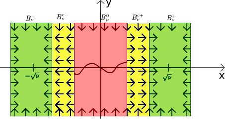
Figure 1: Illustration of the behavior after bifurcation.

Figure 1 illustrates the behavior after bifurcation. We will use the following strategy of the proof (to prove that the connection from zero to the stable equilibrium to the right exists; proof of the existence of the other one is analogous). It is split into three steps.

• Step IIIa – hyperbolicity of the origin after the bifurcation. The proof is realized in Lemma 2.6, where we show that on the red set $B_{\nu}^{0}$ the strong cone conditions are satisfied, hence $0$ is hyperbolic and there exists a point $z_{*}\in B_{\nu}^{c+}\cap W^{u}_{B_{\nu}^{0}}(0)$, where $B_{\nu}^{c+}$ is the blue set to the right in the picture.

• Step IIIb – connection sets. The proof is realized in Lemma 2.7, where we show that on the blue set to the right $B_{\nu}^{c+}$ we have $x^{\prime}>0$, thus there exists a time $t_{1}>0$ such that $\varphi(t_{1},z_{*})\in B_{\nu}^{+}$ (the green set to the right in the picture).

• Step IIIc – hyperbolicity of the born fixed points. The proof is realized in Lemma 2.8, where we show that the green set to the right $B_{\nu}^{+}$ is forward-invariant and for all $z\in B_{\nu}^{+}$ we have $\mu_{2}(DF(z))<l<0$, thus as we have discussed above there exists a unique fixed point $z^{+}\in B_{\nu}^{+}$ and moreover this fixed point is hyperbolic and we have $\lim_{t\to\infty}\varphi(t,\varphi(t_{1},z_{*}))=z^{+}$.

Lemma 2.6 (Step IIIa – hyperbolicity of the origin after the bifurcation).

Let

$$B_{\nu}^{0}:=\left[-\frac{\sqrt{\nu}}{2},\frac{\sqrt{\nu}}{2}\right]\times\left[-\nu,\nu\right].$$

There exists $\nu_{+}>0$ such that for (10) for $\nu\in(0,\nu_{+}]$ the origin is hyperbolic and the unstable manifold $W^{u}_{B_{\nu}^{0}}(0)$ is the image of a horizontal disk in $B_{\nu}^{0}$.

Proof.

Fix $\nu_{+}>0$ and $\nu\in(0,\nu_{+}]$. In Lemma 2.7 we will show that $B_{\nu}^{0}$ is an $\varepsilon$-isolating cuboid for sufficiently small $\nu$. Thus to use Theorems 1.16 and 1.21 it is enough to show that the strong cone conditions are satisfied with the quadratic form given by the matrix

$$Q=\begin{pmatrix}1&0\\ 0&-1\end{pmatrix}.$$

Denote $Q_{\pm\delta}=Q\pm\delta\mbox{Id}\,$. To prove that the strong cone conditions hold, we will show that or $z_{1},z_{2}\in B_{\nu}^{0}$ there exists $\lambda>0$ such that for $\delta>0$ small enough we have

$$\frac{d}{dt}\left(\left(\varphi\left(t,z_{1}\right)-\varphi\left(t,z_{2}\right)\right)^{T}Q_{\pm\delta}\left(\varphi\left(t,z_{1}\right)-\varphi\left(t,z_{2}\right)\right)\right)\Big{|}_{t=0}>\lambda\left(z_{1}-z_{2}\right)^{2}$$

We have

$$\frac{d}{dt} \left(\left(\varphi\left(t,z_{1}\right)-\varphi\left(t,z_{2}\right)\right)^{T}Q_{\pm\delta}\left(\varphi\left(t,z_{1}\right)-\varphi\left(t,z_{2}\right)\right)\right)\Big{|}_{t=0}$$

$$=\left(F_{\nu}\left(z_{1}\right)-F_{\nu}\left(z_{2}\right)\right)^{T}Q_{\pm\delta}\left(z_{1}-z_{2}\right)+\left(z_{1}-z_{2}\right)^{T}Q_{\pm\delta}\left(F_{\nu}\left(z_{1}\right)-F_{\nu}\left(z_{2}\right)\right),$$

We now want to factorize $z_{1}-z_{2}$. Given that denoting $\overline{DF}_{\nu}:=\int_{0}^{1}DF_{\nu}\left(tz_{1}+(1-t)z_{2}\right)\mathrm{d}t$ we have

$$F_{\nu}\left(z_{1}\right)-F_{\nu}\left(z_{2}\right)=\overline{DF}_{\nu}\left(z_{1}-z_{2}\right),$$

thus

$$\frac{d}{dt} \left(\left(\varphi\left(t,z_{1}\right)-\varphi\left(t,z_{2}\right)\right)^{T}Q_{\pm\delta}\left(\varphi\left(t,z_{1}\right)-\varphi\left(t,z_{2}\right)\right)\right)\Big{|}_{t=0}$$

$$=(z_{1}-z_{2})^{T}\left(\overline{DF}_{\nu}^{T}Q_{\pm\delta}+Q_{\pm\delta}\overline{DF}_{\nu}\right)(z_{1}-z_{2})$$

Thus it is sufficient to show that $A=\overline{DF}_{\nu}^{T}Q_{\pm\delta}+Q_{\pm\delta}\overline{DF}_{\nu}$ is positive definite. We see that the eigenvalues of $A$ are bounded from below by

$$\lambda_{1} >2(1-\delta)\inf_{z\in B_{\nu}^{0}}\frac{\partial f_{\nu}}{\partial x}\left(z\right)-(1+\delta)\sup_{z\in B_{\nu}^{0}}\left(\left\lvert\frac{\partial f_{\nu}}{\partial y}\left(z\right)+\frac{\partial g_{\nu}}{\partial x}\left(z\right)\right\rvert\right)$$

$$>2(1-\delta)\nu-(1+\delta)\sup_{z\in B_{\nu}^{0}}\left(3x^{2}+\left\lvert x^{3}+2xy+\frac{5}{2}x^{3}\right\rvert\right)>\frac{\nu}{4}-O(\nu^{\frac{3}{2}})>0,$$

$$\lambda_{2} >2(1-\delta)\inf_{z\in B_{\nu}^{0}}\left(-\frac{\partial g_{\nu}}{\partial y}\left(z\right)\right)-(1+\delta)\sup_{z\in B_{\nu}^{0}}\left\lvert\frac{\partial g_{\nu}}{\partial x}\left(z\right)+\frac{\partial f_{\nu}}{\partial y}\left(z\right)\right\rvert$$

$$>2(1-\delta)-\left(1+\delta\right)\sup_{z\in B_{\nu}^{0}}\left(x^{2}+\left\lvert x^{3}+2xy+\frac{5}{2}x^{3}\right\rvert\right)>2(1-\delta)-O(\nu)>0,$$

if $\nu,\delta$ are small enough. In Lemma 2.7 we will also show that $B_{\nu}^{0}$ is an $\varepsilon$-isolating cuboid. This completes the proof.  

We now prove that on Figure 1 everything from the blue region eventually flows into the green region. It will also show the missing part of the proof above, namely that $B_{\nu}^{0}$ is $\varepsilon$-isolating cuboid for $\nu>0$.

Lemma 2.7 (Step IIIb – connection sets).

There exists $\nu_{+}>0$ such that for each $0<\nu\leq\nu_{+}$ we have

$$x^{\prime} >0,$$ (11)

$$x^{\prime} <0,$$ (12)

respectively on the sets

$$B_{\nu}^{c+} :=\left[\frac{\sqrt{\nu}}{2},\sqrt{\frac{\nu}{2}}\right]\times\left[-\nu,\nu\right],$$

$$B_{\nu}^{c-} :=\left[-\sqrt{\frac{\nu}{2}},-\frac{\sqrt{\nu}}{2}\right]\times\left[-\nu,\nu\right].$$

Proof.

Let $(x,y)\in B_{\nu}^{c+}$ (proof for $B_{\nu}^{c-}$ is analogous). If $\nu>0$ is small enough, then we have

$$x^{\prime}=x(\nu-x^{2})+x^{3}y+xy^{2}>\frac{3}{8}\nu^{\frac{3}{2}}-\left(\frac{1}{2\sqrt{2}}+\frac{1}{\sqrt{2}}\right)\nu^{\frac{5}{3}}>0,$$

since $\nu>0$.  

We now proceed to establishing the basins of attraction in the green ($B_{\nu}^{\pm}$, see Figure 1) neighborhoods of approximate fixed points $(\pm\sqrt{\nu},0)$ of (10).

Lemma 2.8 (Step IIIc – hyperbolicity of the born fixed points).

There exists $\nu_{+}>0$ such that for $0<\nu\leq\nu_{+}$ there exist unique attracting fixed points $u_{\pm}\in B^{\pm}_{\nu}$, where

$$B^{+}_{\nu} :=\left[\sqrt{\frac{\nu}{2}},\sqrt{2\nu}\right]\times\left[-\nu,\nu\right],$$

$$B^{-}_{\nu} :=\left[-\sqrt{2\nu},-\sqrt{\frac{\nu}{2}}\right]\times\left[-\nu,\nu\right].$$

Proof.

The sets $B^{\pm}_{\nu}$ are also easily seen to be forward-invariant.

We proceed to proving that the $l_{2}$ logarithmic norm is negative. We have

$$\frac{DF_{\nu}\left(x,y\right)^{T}+DF_{\nu}\left(x,y\right)}{2}=\begin{pmatrix}\nu-3x^{2}+3x^{2}y+y^{2}&\frac{x^{3}+2xy+2xy+4x^{3}}{2}\\ \frac{x^{3}+2xy+2xy+4x^{3}}{2}&-1+x^{2}\end{pmatrix}.$$

We show that the eigenvalues $\lambda_{1,2}$ of this matrix are negative. If $\nu_{+}$ is small enough, then for $\nu\in[0,\nu_{+}]$, for $(x,y)\in B_{\nu}^{\pm}$ we have $\nu-3x^{2}\leq-\frac{\nu}{2}$

$$\lambda_{1}\leq\nu-3x^{2}+3x^{2}y+y^{2}+\left\lvert\frac{x^{3}+2xy+2xy+4x^{3}}{2}\right\rvert\leq-\frac{\nu}{2}+O(\nu^{\frac{3}{2}})<0,$$

as $\nu>0$. We also obviously have $\lambda_{2}\leq-1+x^{2}+\left\lvert\frac{x^{3}+2xy+2xy+4x^{3}}{2}\right\rvert<0$. Since $B_{\nu}^{\pm}$ are forward-invariant, the conclusion follows by Lemma 9.3.  

We are finally ready to prove the bifurcation theorem for our model.

Theorem 2.9.

There exist $\nu_{-}<0<\nu_{+}$ such that the pitchfork bifurcation occurs in (10) on the interval $\left[\nu_{-},\nu_{+}\right]$.

Proof.

By Lemmas 2.3, 2.6 it remains to show that (P3) is satisfied. Let $\nu_{+}>0$ be small enough and let $0<\nu\leq\nu_{+}$. By Lemma 2.6 there exists such a point $z_{*}=(x_{*},y_{*})\in B_{\nu}^{c+}\cap B_{\nu}^{0}$ which has a backward orbit to $0$. By Lemma 2.7 there exists $T>0$ such that $\varphi_{\nu}(T,z_{*})\in B_{\nu}^{+}$ and by Lemma 2.8 everything in $B_{\nu}^{+}$ is attracted to the fixed point $u_{+}^{\nu}$. This gives us the required heteroclinic connection.

Proof of the connection to $u_{-}^{\nu}$ is analogous.

It remains to show that the fixed points together with the heteroclinic connections constitute the maximal invariant set in $R$. By Lemma 6.4, every point in $R$ flows into $B_{\nu}$. Let us now discuss the backward trajectories of points in $B_{\nu}$. In $B_{\nu}^{0}$ by Lemma 2.6 and Theorem 1.16, only points on the unstable manifold have full-backward trajectory $B_{\nu}^{0}$. Moreover, since $B_{\nu}^{0}$ is an isolating cuboid, for every other point in $B_{\nu}^{0}$ its backward trajectory leaves $B_{\nu}$. Now, in $B_{\nu}^{c+}\cup B_{\nu}^{+}$ every point’s backward trajectory goes into $B_{\nu}^{0}$ or leaves $B_{\nu}$, so only points with the full-backward trajectory are the ones which have $z_{*}$ in the backward trajectory. The conclusion about the maximal invariance easily follows.

 

Observe that the terms of higher order in $F_{\nu}$ (i.e. $f_{\nu}$ terms of form $x^{k}y^{l}$ for $k>3$ or $l>3$ and terms of form $x^{k}y^{l}$ for $k>2$ and $l\geq 1$ or for $k\geq 4$ in $g_{\nu}$) would not change our proof of the bifurcation in any meaningful way.

However, terms like $xy$ and $x^{2}y$ in $f_{\nu}$ or $y^{2}$ and $x^{3}$ in equation for $g_{\nu}$ would, as in $DF_{\nu}$ they would give rise respectively to $x$ and $2y$. Because of such terms, $\nu-3x^{2}$ would no longer be dominating in $DF_{\nu}$ and the presented reasoning would not work. Such terms do appear in the Kuramoto–Sivashinsky equation written in the Fourier basis.

We could deal with those terms by taking different shapes of sets, but it is a very unwieldy approach. Instead, in Section 6.1, using the normal form theory we present coordinate changes which remove those terms, introducing instead other terms of higher order, which in turn pose no problem to our approach.

We did not consider the term $y^{2}$ (in the equation for $x^{\prime}$) in this model. It also could be removed by the change of coordinates, but it would also suffice to take different shape of sets in the proof – we elaborate on this approach in the proof in the model given below, which arise there because of the term $yz$, where $z$ will be another direction different from the bifurcation direction. Although those terms could also be removed in a finite-dimensional case, in the Kuramoto–Sivashinsky there are infinitely many terms of such form, which is why we will present an argument with the changed shape of sets.

2.3 Bifurcation model with an unstable direction

2.3.1 Statement of the model and outline of the proof

Now we will briefly discuss the changes which occur when we add an unstable direction. Consider the following equation

$$\begin{split}x^{\prime}&=x\left(\nu-x^{2}\right)+x^{3}\left(y+z\right)+x\left(y^{2}+z^{2}\right)+yz,\\ y^{\prime}&=y+x^{2}\left(y+z\right)+x^{4}+yz,\\ z^{\prime}&=-z+x^{2}\left(y+z\right)+x^{4}+yz.\end{split}$$ (13)

The proof in this case proceeds similarly to the proof in the previous model, although there are some differences which we ought to stress before we proceed to the details of the proof.

In the previous model when proving Step I we descended through the family of the forward-invariant sets closer and closer to the origin. Of course, because of the unstable direction it is impossible now. This is why now we flow through the descending family of the isolating cuboids. The details of this flow are only a bit more complicated than in the previous model. Before the bifurcation we get every point in $R$ either leaves $R$ or flows to the origin in the limit. Similarly, after the bifurcation every point either flows out of $R$ or flows into $B_{\nu}$. We know even more – if a point leaves $B_{\nu}$, then it necessarily leaves $R$. We thus see that as before to describe the dynamics after the bifurcation completely, we just need to describe the dynamics on $B_{\nu}$.

When it comes to Step II, i.e. proving the hyperbolicity before the bifurcation, we can no longer use the logarithmic norms because of the unstable direction. But it does not change much, as verifying the strong cone conditions relies on very similar calculations (unsurprising, because negativity of the $l_{2}$ logarithmic norm is in a special case of the cone conditions).

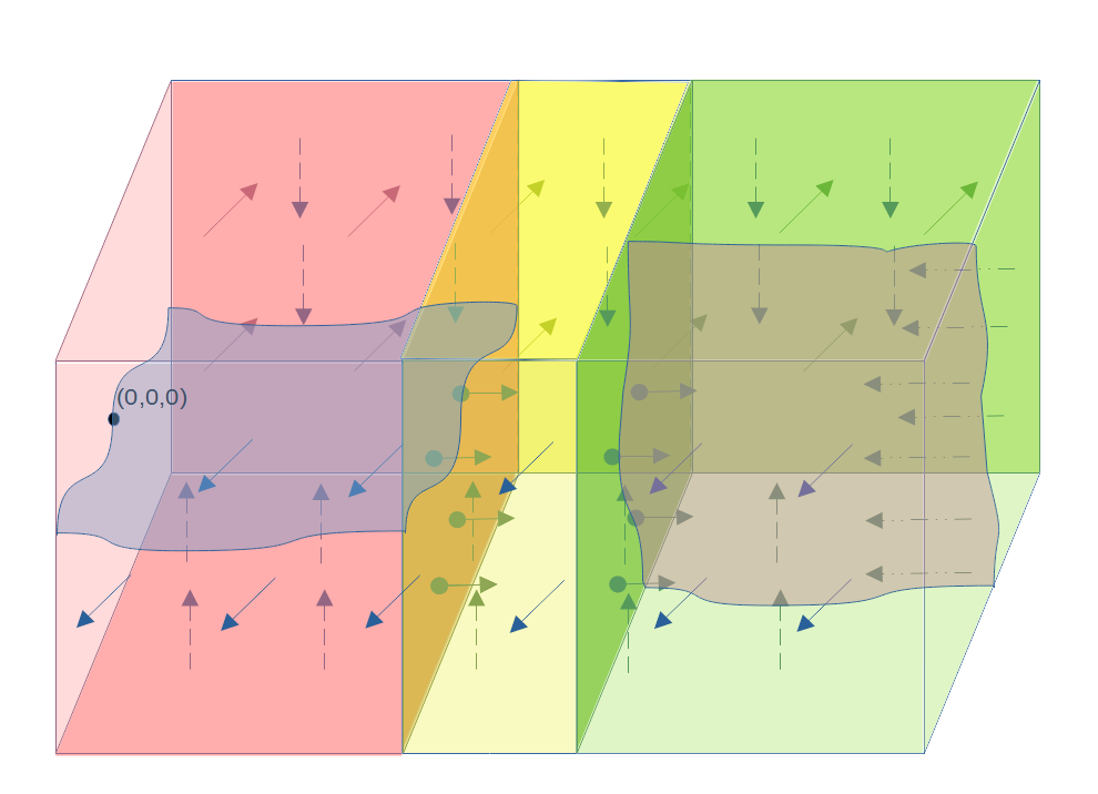
Figure 2: Illustration of the proof of the heteroclinic connection when there is an unstable direction. The red set is the set $B_{\nu}^{0}$, in which we verify the cone conditions to get the unstable manifold (the blue surface). In the yellow set $B_{\nu}^{c+}$ we have growth in the bifurcation direction. The green set is $B_{\nu}^{0}$, in which we brown surface is the stable manifold which we again get by the cone conditions.

The illustration of the proof after the bifurcation is in the Figure 2 (one side, as previously the other one is analogous). $B_{\nu}^{0},B_{\nu}^{c+},B_{\nu}^{+}$ refer respectively to the red, yellow and green set in the picture. The set $B_{\nu}^{ct+}$ is the sum $B_{\nu}^{c+}\cup B_{\nu}^{+}$.

As before, in Step IIIa we use the cone conditions to establish that the unstable manifold of the origin is a graph. However, after the bifurcation, this manifold close to the origin (blue surface in the picture) is a graph over not only the bifurcation direction $x$, but also the over the additional unstable direction $y$, hence it is two-dimensional. So while in the previous model its intersection with the exit set of the isolating cuboid close to the origin was a point (for each of the ’branches’ of the manifold), now it is a graph over the unstable direction $y$ (see the intersection $W^{u}_{B_{\nu}^{0}}(0)\cap B_{\nu}^{c+}$, i.e. of the blue surface with the yellow set).

Previously in Step IIIb we could propagate the point from the unstable manifold on the exit set close to the fixed point that was born simply by propagating the entire exit set. Now it does not work, because not every point from this exit set flows close to the target fixed point. However, we prove that on $B_{\nu}^{ct+}$ the cones given by the matrix

$$\begin{pmatrix}&-1&0&0\\ &0&1&0\\ &0&0&-1\end{pmatrix}.$$

are forward-invariant. Together with the fact that on $B_{\nu}^{c+}$ we have $x^{\prime}>0$ it gives us that there is a subset $W^{\prime}\subset W^{u}_{B_{\nu}^{0}}(0)\cap B_{\nu}^{c+}$ such that for some time $T>0$ we have that $H:=\varphi_{\mu}(T,W^{\prime})\subset B_{\nu}^{+}$ is a graph over the $y$ direction. As we will see in the moment, $H$ intersects with the stable manifold.

Next, we proceed to the Step IIIb in which we verify the cone conditions on the set $B_{\nu}^{+}$ and conclude that

• there exists a hyperbolic fixed point $z_{\nu}^{+}\in B_{\nu}^{+}$,

• there exists exactly one point on $H$ which converges to $z_{\nu}^{+}$ forward in time; it gives us the required heteroclinic connection,

• the unstable (stable) manifold $W^{u}_{B_{\nu}^{+}}(z_{\nu}^{+})$($W^{s}_{B_{\nu}^{+}}(z_{\nu}^{+})$) is a graph over the $y$ direction (over the $x,z$ directions); we need those facts to prove that the heteroclinic connections constitute the maximal invariant set.

2.3.2 Details of the proof

We proceed to the details of the proof. Denote

$$B_{\nu}:=\left[-\sqrt{2\nu},\sqrt{2\nu}\right]\times\left[-\nu^{\frac{3}{2}},\nu^{\frac{3}{2}}\right]^{2}.$$

We also denote the form given by the matrix

$$Q_{1}=\begin{pmatrix}&1&0&0\\ &0&1&0\\ &0&0&-1\end{pmatrix}$$

by $\mathcal{Q}_{1}$ and the form given by the matrix

$$Q_{2}=\begin{pmatrix}&-1&0&0\\ &0&1&0\\ &0&0&-1\end{pmatrix}.$$

by $\mathcal{Q}_{2}$.

We now prove that all dynamics near the bifurcation can be isolated. We start with the case after the bifurcation.

Lemma 2.10 (Step I – existence of the set isolating the bifurcation, situation after the bifurcation).

There exists $\nu_{+}>0$ such that for $\nu\in(0,\nu_{+}]$ we have that for all $u\in R:=B_{\nu_{+}}$ either $u$ leaves $R$ or there exists $t>0$ such that $\varphi\left(t,u\right)\in B_{\nu}$. Moreover, if a point $u\in B_{\nu}$ leaves $B_{\nu}$, then it also leaves $R$.

Proof.

Fix $\nu>0$ and $\theta\in\left[\nu,\nu_{+}\right]$, where $\nu_{+}$ is small enough. Defining $\theta^{\prime}=\max\left\{\frac{\theta}{2},\nu\right\}$ we will show that every point $u\in S_{\theta}\setminus S_{\theta^{\prime}}$ flows into $S_{\theta^{\prime}}$ or leaves $R$. First let us fix $(x,y,z)=u\in S_{\theta}\setminus S_{\theta^{\prime}}$ and look at the vector field. We can prove analogously as in Lemma 2.3 that ${\rm sgn}\,x^{\prime}=-{\rm sgn}\,x,{\rm sgn}\,z^{\prime}=-{\rm sgn}\,z$ and ${\rm sgn}\,y^{\prime}={\rm sgn}\,y$. Now observe that it easily implies if there exists sufficiently big $T>0$ such that for all $t\in\left[0,T\right]$ we have $\left\lvert\pi_{y}\varphi(t,u)\right\rvert<\theta^{\prime\frac{3}{2}}$, then we have $\varphi\left(T,u\right)\in S_{\theta^{\prime}}$. Thus to prove the lemma it is enough to show that if for some $t>0$ we have $\left\lvert\pi_{y}\varphi(t,u)\right\rvert\geq\theta^{\prime\frac{3}{2}}$, then we leave $R$. In this case we leave $S_{\theta}$ because $\left\lvert y\right\rvert$ increases, so we can never go into $S_{\theta^{\prime}}$. But once we leave then we have a point in $S_{\min\left\{\nu_{+},2\theta\right\}}\setminus S_{\theta}$ such that for it $\left\lvert y\right\rvert=\theta^{\frac{3}{2}}$, so for analogous reasons it leaves $S_{\min\left\{\nu_{+},2\theta\right\}}$ and so on until we leave $R$.  

Slightly modifying the proof above, we get the following lemma about the situation before the bifurcation.

Lemma 2.11 (Step I – existence of the set isolating the bifurcation, situation before the bifurcation).

There exist $\nu_{-}<0<\nu_{+}$ such that for each $\nu\in\left[\nu_{-},0\right]$ we have that for all $u\in R:=B_{\nu_{+}}$ either $u$ leaves $R$ or we have $\varphi\left(t,u\right)\to 0$.

Now we state the hyperbolicity result. Compared to the proof of the Lemma 2.6, we need to use the cone conditions instead of the logarithmic norms in the proof of the hyperbolicity before the bifurcation (because of the additional unstable direction). Nevertheless, the computations are almost the same, so we skip them.

Lemma 2.12 (Step II and IIIa – hyperbolicity of the origin before and after the bifurcation).

There exists $\nu_{-}<0<\nu_{+}$ such that for (13) the origin is hyperbolic for $\nu\in\left[\nu_{-},\nu_{+}\right]\setminus\left\{0\right\}$. Moreover, for $\nu\in(0,\nu_{+}]$ the unstable manifold $W^{u}_{B_{\nu}^{0}}(0)$, where $B_{\nu}^{0}:=\left[-\frac{\sqrt{\nu}}{2},\frac{\sqrt{\nu}}{2}\right]\times\left[-\nu^{\frac{3}{2}},\nu^{\frac{3}{2}}\right]^{2}$, is the image of a horizontal disk in $B_{\nu}^{0}$ with respect to the cones given by $\mathcal{Q}_{1}$.

Now we proceed to proving that although not all points from the set $B_{\nu}^{0}\cap B_{\nu}^{c\pm+}$ flow into $B_{\nu}^{\pm}$, we can nevertheless say that the image of some subset of $W^{u}_{B_{\nu}^{0}}\cap B_{\nu}^{c\pm}$ is a graph over the unstable direction $y$ in the set $B_{\nu}^{+}$.

Lemma 2.13 (Step IIIb – connection sets, cone invariance).

If $\nu>0$ is small enough, then the sets

$$B_{\nu}^{ct+} :=\left[\frac{\sqrt{\nu}}{2},\sqrt{2\nu}\right]\times\left[-\nu^{\frac{3}{2}},\nu^{\frac{3}{2}}\right]^{2},$$

$$B_{\nu}^{ct-} :=\left[-\sqrt{2\nu},\frac{\sqrt{\nu}}{2}\right]\times\left[-\nu^{\frac{3}{2}},\nu^{\frac{3}{2}}\right]^{2}.$$

are $\varepsilon-$isolating cuboids. Moreover, if $h$ is a horizontal disk with respect to the cones $\mathcal{Q}_{2}$ in $B_{\nu}^{ct\pm}$, then $\varphi_{\mu}\left(t,h\left(\pi_{y}B_{\nu}^{ct\pm}\right)\right)$ contains the image of another horizontal disk with respect to the cones $\mathcal{Q}_{2}$ for all $t>0$.

Proof.

We will verify the assumptions of Lemma 1.13. First we check that those sets are indeed $\varepsilon$-isolating cuboids. Let $(x,y,z)\in B_{\nu}^{ct+}.$ Then if $\nu$ is small enough we can find $d>0$ such that for all $(x,y,z)$ with $y=\nu^{\frac{3}{2}}$ (case $y=-\nu^{\frac{3}{2}}$ is analogous) we have

$$y^{\prime} =y+x^{2}\left(y+z\right)+x^{4}+yz\geq$$

$$\geq\nu^{\frac{3}{2}}-O\left(\nu^{\frac{5}{2}}+\nu^{2}+\nu^{3}\right)>0.$$

Thus we see that we can pick $\varepsilon$ such that the condition the condition (I2) holds.

Proper behavior on $x,z$ directions can be checked by the computations as in the previous model.

Now we verify the remaining assumption of the Lemma 1.13, i.e. that the positive cones are invariant. We do this by showing that if $\mathcal{Q}_{2}\left(\varphi\left(t,u_{1}\right)-\varphi\left(t,u_{2}\right)\right)>0$, then $\frac{d}{dt}\mathcal{Q}_{2}\left(\varphi\left(t,u_{1}\right)-\varphi\left(t,u_{2}\right)\right)\Big{|}_{t=0}>0$.

As in the proof of Lemma 2.6, we get that for $u_{1},u_{2}\in B_{\nu}^{ct+}$ and defining $A:=\overline{DF}_{\nu}^{T}Q_{2}+Q_{2}\overline{DF}_{\nu}$

$$\frac{d}{dt}\left(\varphi\left(t,u_{1}\right)-\varphi\left(t,u_{2}\right)\right)^{T}Q_{2}\left(\varphi\left(t,u_{1}\right)-\varphi\left(t,u_{2}\right)\right)=(u_{1}-u_{2})^{T}A(u_{1}-u_{2}).$$

Denote $u_{1}-u_{2}=:\left(x,y,z\right)$. Then we can symbolically write

$$(u_{1}-u_{2})^{T}A(u_{1}-u_{2})=\sum_{a,b\in\left\{x,y,z\right\}}A_{ab}ab.$$

Now what we will show is that $A_{yy},A_{zz}>0$ and that $A_{yy}$ dominates $A_{xx}$ (which on some part of the set is negative) and all off-diagonal $A$ terms. Then, considering that $\mathcal{Q}_{2}\left(u_{1}-u_{2}\right)>0$ is equivalent to $y^{2}>x^{2}+z^{2}$, we have for sufficiently small $\nu>0$ (ignoring a non-negative term $A_{zz}z^{2}$).

$$\sum_{a,b\in\left\{x,y,z\right\}}A_{ab}ab>\left(A_{yy}-\left\lvert A_{xx}\right\rvert-\sum_{a,b\in\left\{x,y,z\right\},a\neq b}\left\lvert A_{ab}\right\rvert\right)y^{2}>0.$$

Thus we calculate

$$A_{xx} \geq\nu-3x^{2}-\sup_{u\in B_{\nu}^{ct+}}\left(3x^{2}\left(y+z\right)+y^{2}+z^{2}\right)\geq-5\nu-O(\nu^{\frac{5}{2}}),$$

$$A_{yy} \geq 1-\sup_{u\in B_{\nu}^{ct+}}\left(x^{2}+z\right)=1-O(\nu)>0,$$

$$A_{zz} \geq 1-\sup_{u\in B_{\nu}^{ct+}}\left(x^{2}+y\right)=1-O(\nu)>0.$$

We see that we can similarly show that the off-diagonal terms are all at worst $O(\nu)$ and thus we have shown what we wanted to. We also see that the bounds do not depend on the choice of $u_{1},u_{2}$.  

The proof of result about the growth in the bifurcation direction almost does not change, so we skip it.

Lemma 2.14 (Step IIIb – connection sets, growth in the bifurcation direction).

We have

$$x^{\prime} >0,$$

$$x^{\prime} <0,$$

respectively on the sets

$$B_{\nu}^{c+} :=\left[\frac{\sqrt{\nu}}{2},\frac{\sqrt{\nu}}{\sqrt{2}}\right]\times\left[-\nu^{\frac{3}{2}},\nu^{\frac{3}{2}}\right]^{2},$$

$$B_{\nu}^{c-} :=\left[-\frac{\sqrt{\nu}}{\sqrt{2}},\frac{\sqrt{\nu}}{2}\right]\times\left[-\nu^{\frac{3}{2}},\nu^{\frac{3}{2}}\right]^{2}.$$

The following lemma states that the new fixed points are indeed born and that they are hyperbolic. Moreover, their stable manifolds are graphs over $x,z$ directions. To prove this it is enough to verify the cone conditions and use the Theorem 1.15, so the computations are again skipped.

Lemma 2.15 (Step IIIc – hyperbolicity of the born fixed points).

There exists $\nu_{+}>0$ such that for $0<\nu\leq\nu_{+}$ there exist unique fixed points $u^{\pm}_{\nu}\in B^{\pm}_{\nu}$, where

$$B^{+}_{\nu} :=\left[\sqrt{\frac{\nu}{2}},\sqrt{2\nu}\right]\times\left[-\nu^{\frac{3}{2}},\nu^{\frac{3}{2}}\right]^{2},$$

$$B^{-}_{\nu} :=\left[-\sqrt{2\nu},-\sqrt{\frac{\nu}{2}}\right]\times\left[-\nu^{\frac{3}{2}},\nu^{\frac{3}{2}}\right]^{2}.$$

Moreover, those fixed points are hyperbolic with respect to the cones given by $\mathcal{Q}_{2}$ and $W^{u}_{B^{\pm}_{\nu}}\left(u^{\pm}_{\nu}\right)$ ($W^{s}_{B^{\pm}_{\nu}}\left(u^{\pm}_{\nu}\right)$) are the images of horizontal (vertical) disks.

We are ready to prove that the bifurcation occurs in the model with an unstable direction.

Theorem 2.16.

There exist $\nu_{-}<0<\nu_{+}$ such that the pitchfork bifurcation occurs in (13) on the interval $\left[\nu_{-},\nu_{+}\right]$.

Proof.

Observe that by Lemma 2.12 the unstable manifold $W^{u}_{B_{\nu}^{0}}$ is the image of a horizontal disk with respect to cones $\mathcal{Q}_{1}$, thus the set $W^{*}:=W^{u}_{B_{\nu}^{0}}\cap B_{\nu}^{c+}$ is clearly the image of a horizontal disk in $B_{\nu}^{ct+}$ with respect to the cones $\mathcal{Q}_{2}$. Thus due to the Lemmas 2.13 and 2.14 we get that there exists a time $T>0$ such that $\varphi\left(T,W^{*}\right)$ is the image of some horizontal disk in $B_{\nu}^{+}$, which we denote by $h$. Thus by Lemmas 2.15 and 1.14 we get that for some $u\in h(\pi_{y}B_{\nu}^{+})$ we have $\lim_{t\to\infty}\varphi(t,u)=z_{+}$.

It remains to show that we have obtained the maximal invariant set. By Lemma 2.10, we only need to focus on $B_{\nu}$ for $\nu>0$ (case $\nu\leq 0$ being obvious).

Observe that by Lemma 1.16 and by the fact that $B_{\nu}^{0}$ is an $\varepsilon$-isolating cuboid, every point in $B_{\nu}^{0}$ leaves $B_{\nu}$ backward in time or is on the unstable manifold, so only points in $B_{\nu}^{0}$ which can be in the maximal invariant set are the points from $W^{u}_{S_{\nu}^{0}}\left(0\right)$.

Points in the sets $B_{\nu}^{\pm}$ backward in time either leave $B_{\nu}$ or go into $B_{\nu}^{0}$. Thus only those points which have some point from $W^{u}_{S_{\nu}^{0}}\left(0\right)$ on their backward trajectory can be in the maximal invariant set.

Now consider $u\in B_{\nu}^{\pm}$. Then this point’s backward trajectory may

• leave $B_{\nu}$, so it is not in the maximal invariant set.

• stay in $B_{\nu}$. Then $u\in W^{u}_{B_{\nu}^{\pm}}(u_{\nu}^{\pm})$. Now, forward in time $u$ either leaves $B_{\nu}$, so it is not in the maximal invariant set, or stays in $B_{\nu}^{\pm}$. So for $u$ to be in the maximal invariant set, we would also need to have $u\in W^{s}_{B_{\nu}^{\pm}}(u_{\nu}^{\pm})$, thus by Lemma 2.15 we have $u=u_{\nu}^{\pm}$, because horizontal and vertical disk can intersect only in one point.

• flow into $B_{\nu}^{c+}$, so all we have said before applies.

 

3 The method of self-consistent bounds

In this section we recall the method of self-consistent bounds developed in [12, 13, 14]. Let $H\subset L^{2}$ be a real Hilbert space. We study the following equation

$$\frac{du}{dt}=F(u)$$ (14)

where the domain of $F$ is dense in $H$. By a solution of (14) we understand a function $u:[0,t_{max})\to\,{\rm dom}\,(F)$ such that $u$ is differentiable and (14) is satisfied for all $t\in[0,t_{max})$. The scalar product in $H$ will be denoted by $(u|v)$ and norm by $\left\lVert u\right\rVert$, for $u,v\in H$. Throughout this section we assume that there is a set $I\subset\mathbb{Z}^{d}$ and a sequence of subspaces $H_{k}\subset H$ for $k\in I$ such that $\dim H_{k}=d_{k}<\infty$ and $H_{k}$ and $H_{k^{\prime}}$ are mutually orthogonal for $k\neq k^{\prime}$. Let $A_{k}:H\to H_{k}$ be the orthogonal projection onto $H_{k}$. We assume that for each $u\in H$ holds

$$u=\sum_{k\in I}u_{k},$$ (15)

where $u_{k}:=A_{k}u$. Analogously, for a function $B$ with its range in $H$ we set $B_{k}(u):=A_{k}B(u)$ (in particular, $F_{k}(u)=A_{k}F(u)$). Equation (15) implies that $H=\overline{\bigoplus_{k\in I}H_{k}}$.

For $k\in\mathbb{Z}^{d}$ we define

$$\left\lvert k\right\rvert=\sqrt{\sum_{i=1}^{d}k_{i}^{2}}$$

For $n>0$ we set

$$X_{n} =\bigoplus_{\left\lvert k\right\rvert\leq n,k\in I}H_{k}$$

$$Y_{n} =X_{n}^{\bot}.$$

By $P_{n}:H\to X_{n}$ and $P_{n}^{\perp}:H\to Y_{n}$ we will denote the orthogonal projections onto $X_{n}$ and onto $Y_{n}$, respectively.

Definition 3.1.

We say that $F:H\supset\,{\rm dom}\,(F)\to H$ is admissible if the following conditions are satisfied for any $i,j\in I$, such that $\dim X_{i},\dim X_{j}>0$

• $X_{i}\subset\,{\rm dom}\,(F)$,

• $P_{i}F:X_{i}\to X_{i}$ is a $C^{1}$ function,

• $\frac{\partial F_{i}}{\partial x_{j}}$ exists and is continuous.

Definition 3.2.

Assume $F$ is admissible. For a given number $n>0$ the ordinary differential equation

$$x^{\prime}=P_{n}F(x),\textnormal{ where }x\in X_{n},$$ (16)

will be called the $n$-th Galerkin projection of (14).

By $\varphi^{n}(t,x)$ we denote the local flow on $X_{n}$ induced by (16).

Definition 3.3.

Assume $F$ is an admissible function. Let $m,M\in\mathbb{N}$ with $m\leq M$. Consider a compact set $W\subset X_{m}$ and a sequence of compact sets $B_{k}\subset H_{k}$ for $\left\lvert k\right\rvert>m$, $k\in I$. We say that $W\oplus\Pi_{k\in I,\left\lvert k\right\rvert>m}B_{k}$ forms self-consistent bounds for $F$ if

• For $k\in I$ such that $\left\lvert k\right\rvert>M$ we have $0\in B_{k}$ .

• Let $\hat{a}_{k}:=\max_{a\in B_{k}}\left\lVert a\right\rVert$ for $\left\lvert k\right\rvert>m$, $k\in I$. Then $\sum_{\left\lvert k\right\rvert>m,k\in I}\hat{a}_{k}^{2}<\infty$. In particular

  $$W\oplus\Pi_{\left\lvert k\right\rvert>m}B_{k}\subset H$$

  and for every $u\in W\oplus\Pi_{k\in I,\left\lvert k\right\rvert>m}B_{k}$ holds, $\left\lVert P_{n}^{\perp}u\right\rVert\leq\sum_{\left\lvert k\right\rvert>n,k\in I}\hat{a}_{k}^{2}$.

• The function $u\mapsto F(u)$ is continuous on $W\oplus\prod_{k\in I,\left\lvert k\right\rvert>m}B_{k}\subset H$. Moreover, if for $k\in I$ we define $F_{k}=\max_{u\in W\oplus\prod_{k\in I,\left\lvert k\right\rvert>m}B_{k}}\left\lVert F_{k}(u)\right\rVert$, then $\sum F_{k}^{2}<\infty$.

• For $|k|>m$, $k\in I$ $B_{k}$ is given by

  $$B_{k} =[a_{k}^{-},a_{k}^{+}],\qquad a_{s}^{-}<a_{s}^{+},\>s=1,\dots,d_{1}$$ (17)

  Let $u\in W\oplus\Pi_{|k|>m}B_{k}$. Then for $|k|>m$

  $$u_{k}=a_{k}^{-} \Rightarrow F_{k}(u)>0,$$ (18)

  $$u_{k}=a_{k}^{+} \Rightarrow F_{k}(u)<0.$$ (19)

The equations (18, 19) are called isolation equations. In our case those equations will be verified alongside with the proof that the set is forward-invariant or an isolating cuboid.

If the choice of $F$ is clear from the context, then we often drop $F$ and we will speak simply about self-consistent bounds.

Given self-consistent bounds $W$ and $\{B_{k}\}_{k\in I,\left\lvert k\right\rvert>m}$, by $T$ (the tail) we will denote

$$T:=\prod_{\left\lvert k\right\rvert>m}B_{k}\subset Y_{m}.$$

4 Convergence of the Galerkin projections

In this section we get the existence of the (local) semiflows for the self-consistent bounds which are forward-invariant or which are isolating cuboids. We also get that if every Galerkin projection of the self-consistent bounds is forward invariant or an isolating cuboid, then the same is true for the set itself.

We now list two theorems about the convergence of the Galerkin projections, a global version in a forward-invariant set and a local one in an isolating cuboid. We cite here slightly modified result [13, Theorem 13]. Proof of this theorem in [13] is based on logarithmic norms (defined and discussed in Appendix 9), but it is done only for the $l_{2}$ norm. In the computer-assisted proof of the heteroclinic connections we use the max norm, so we rephrase this theorem to work for every logarithmic norm. We discuss it in a bit more detailed way in Appendix 9.

The following condition tells us that the logarithmic norms of the projections are uniformly bounded. It is the most important condition in proving the convergence of the Galerkin projections.

Definition 4.1.

Consider self-consistent bounds $V$ for $F$. We define the following condition

• there exists $l\in\mathbb{R}$ such that for any any $n\in\mathbb{N}$ we have

  $$\mu\left(DP_{n}F\right)<l.$$

By Theorem 9.2, we easily get the following way of verifying the (D) condition.

Lemma 4.2.

Let $R\subset H$ be convex self-consistent bounds for $F$. If there exist $l\in\mathbb{R}$ such that and for all $i\in I$and $x\in R$ we have

• for norm $\left\lVert\cdot\right\rVert=\left\lVert\cdot\right\rVert_{2}$ is the $l_{2}$ norm

  $$\frac{\partial F_{i}}{\partial x_{i}}\left(x\right)+\sum_{k,\>k\neq i}\frac{1}{2}\left(\left\lvert\frac{\partial F_{i}}{\partial x_{k}}(x)\right\rvert+\left\lvert\frac{\partial F_{k}}{\partial x_{i}}(x)\right\rvert\right)\leq l.$$

  then the condition (D) holds with the $l_{2}$ norm.

• for the maximum norm $\left\lVert\cdot\right\rVert=\left\lVert\cdot\right\rVert_{\infty}$

  $$\frac{\partial F_{i}}{\partial x_{i}}(x)+\sum_{k,\>k\neq i}\left\lvert\frac{\partial F_{i}}{\partial x_{k}}(x)\right\rvert\leq l,$$

  then the condition (D) holds with the maximum norm.

We now proceed to the proof of the convergence on the forward-invariant self-consistent bounds. We start by defining the forward-invariance.

Definition 4.3.

We say than a closed set $R\subset X$ is forward-invariant with respect to the semiflow $\varphi$ if for all $x\in R$ and $t\in\mathbb{R}_{+}$ we have $\varphi(t,x)\in R$.

Theorem 4.4.

Assume that $\left\lVert\cdot\right\rVert$ is the $l_{2}$ or the maximum norm on $H$ and let $\mu$ be the associated logarithmic norm. Let $R\subset H$ be a convex self-consistent bounds for $F$ such that the condition (D) holds on $R$.

Assume that $P_{n}(R)$ is forward-invariant for the $n$-dimensional Galerkin projection of (14) for all $n>M$. Then

• Uniform convergence and existence. For a fixed $x_{0}\in R$, let $x_{n}:[0,\infty]\to P_{n}(R)$ be a solution of $x^{\prime}=P_{n}(F(x))$, $x(0)=P_{n}x_{0}$. Then $x_{n}$ converges uniformly on compact intervals to a function $x^{*}:[0,\infty]\to R$, which is a solution of (14) and $x^{*}(0)=x_{0}$. The convergence of $x_{n}$ on compact time intervals is uniform with respect to $x_{0}\in R$.

• Uniqueness within $R$. There exists only one solution of the initial value problem (14), $x(0)=x_{0}$ for any $x_{0}\in R$, such that $x(t)\in R$ for $t>0$.

• Lipschitz constant. Let $x:[0,\infty]\to R$ and $y:[0,\infty]\to R$ be solutions of (14), then

  $$\left\lVert y(t)-x(t)\right\rVert\leq e^{lt}\left\lVert x(0)-y(0)\right\rVert$$ (20)

• Semiflow. The map $\varphi:\mathbb{R}_{+}\times R\to R$, where $\varphi(\cdot,x_{0})$ is a unique solution of equation (14), such that $\varphi(0,x_{0})=x_{0}$ defines a semiflow on $R$.

The following theorem is our main tool in proving the existence of the attracting fixed points.

Theorem 4.5.

[14, Theorem 3.8] Let same assumptions on $R$ and $F$ as in Theorem 4.4 hold. Assume that $l<0$. Then there exists a unique fixed point $x^{*}\in R$ for (14). Moreover, for every $y\in R$

$$\left\lVert\varphi(t,y)-x^{*}\right\rVert \leq e^{lt}\left\lVert y-x^{*}\right\rVert,\textnormal{for }t\geq 0,$$

$$\lim_{t\to\infty}\varphi(t,y) =x^{*}.$$

Remark 4.6.

Observe that if we equip $H$ with $l_{2}$ norm, then the attracting fixed point $x^{*}$ in Theorem 4.5 is hyperbolic in the sense of Definition 1.18. To prove this it is enough to apply Theorem 1.21 with the $l_{2}$ norm and $\mathcal{Q}=-\operatorname{id}$.

The fact that $R$ is forward-invariant was essential in proof of Theorem 4.4 to ensure that the solutions stay in $R$ for all times $t>0$. Nevertheless, if we only could assume that $\varphi(t,x)$ stay in $R$ for times $0\leq t\leq t(x)$, the inequality (20) would still be valid for those times. Thus, a slight modification of the proof of [13, Theorem 13] yields the proof of the following result.

Theorem 4.7.

Assume that $\left\lVert\cdot\right\rVert$ is the $l_{2}$ or the maximum norm on $H$ and let $\mu$ be the associated logarithmic norm. Let $m\leq M$ be natural numbers. Let $c_{u}:X_{m}\to\mathbb{R}^{m}$ be a homeomorphism and consider the self-consistent bounds for $F$ of the form $V:=c_{u}^{-1}(\overline{B}(0,1))\oplus\bigoplus_{k=m+1}^{\infty}B_{k}$. Assume that there exists $\varepsilon>0$ such that for each $n>M$ the set $P_{n}\left(V\right)=c_{u}^{-1}(\overline{B}(0,1))\oplus\bigoplus_{i=m+1}^{n}B_{k}$ is an $\varepsilon$-isolating cuboid for $\varphi_{n}$. Moreover, assume that the condition (D) holds for $V^{\varepsilon}:=c_{u}^{-1}(\overline{B}(0,1+\varepsilon))\oplus\bigoplus_{i=m+1}^{\infty}B_{k}$.

Then

• Local uniform convergence and existence For a fixed $x_{0}\in V^{\varepsilon}$, let $x_{n}:[0,t_{max}(n,x_{0})]\to P_{n}(V)^{\varepsilon}$ be a solution of $x^{\prime}=P_{n}(F(x))$, $x(0)=P_{n}x_{0}$ defined on the maximum interval of existence. Then $t_{\max}(n,x_{0})\to t_{\max}(x_{0})$ and $x_{n}$ converges uniformly on compact intervals contained in $\left[0,t_{\max}(x_{0})\right]$ to a function $x^{*}:\left[0,t_{max}(x_{0})\right]\to V^{\varepsilon}$, which is a solution of (14) and for which $x^{*}(0)=x_{0}$. The convergence of $x_{n}$ on compact time intervals is uniform with respect to $x_{0}\in V^{\varepsilon}$.

• Uniqueness within $V^{\varepsilon}$. For any $x_{0}\in V^{\varepsilon}$ there exists only one solution of the initial value problem (14), $x(0)=x_{0}$ such that $x(t)\in V^{\varepsilon}$ for $0<t<t_{\max}(x_{0})$.

• Lipschitz constant. Let $x:[0,t_{1}]\to V^{\varepsilon}$ and $y:[0,t_{1}]\to V^{\varepsilon}$ be solutions of (14), then

  $$\left\lVert y(t)-x(t)\right\rVert\leq e^{lt}\left\lVert x(0)-y(0)\right\rVert.$$

• Local semiflow. The partial map $\varphi:\mathbb{R}_{+}\times H\rightharpoonup H$, where $\varphi(\cdot,x_{0})$ is the unique solution of equation (14) such that $\varphi(0,x_{0})=x_{0}$, defines a local semiflow on $V$.

• Isolation. The set $V$ is an $\varepsilon$-isolating cuboid for $\varphi$.

For set $V$ as in theorem above we call directions $\left\{1,\ldots,m\right\}$ the exit and the remaining directions the entry directions.

5 Verification of the cone conditions

We will need a slight modification of Lemma 3.1 proved in [15].

Lemma 5.1.

Let $V\subset H$ be self-consistent bounds for an admissible function $F$. Moreover, assume that the following condition holds.

• if we set $d_{ij}:=\max_{x\in V}\left\lvert\frac{\partial F_{i}}{\partial x_{j}}\right\rvert$, then for each $i\in\mathbb{N}$ the sum

  $$\sum_{j=1}^{\infty}d_{ij}\sup_{x,y\in V}\left\lvert x_{j}-y_{j}\right\rvert$$

  converges.

Then for all $x,y\in V$ we have

$$F(x)-F(y)=\overline{DF}\left(x-y\right),$$

where

$$\overline{DF}_{ij}:=\int_{0}^{1}\frac{\partial F_{i}}{\partial x_{j}}\left(tx+\left(1-t\right)y\right)\,\mathrm{d}t.$$

Proof.

By Lemma 3.1 from [15], we have

$$F_{i}(x)-F_{i}(y)=\sum_{j=1}^{\infty}\int_{0}^{1}\frac{\partial F_{i}}{\partial x_{j}}\left(tx+\left(1-t\right)y\right)\,\mathrm{d}t\left(x_{j}-y_{j}\right).$$

Thus, it is enough to prove that $P_{n}F(x)-P_{n}F(y)\to F(x)-F(y)$, which immediately follows by (C3).  

Theorem 5.2.

Let $V$ be self-consistent bounds for $F$ and assume that $F$ defines a continuous local semiflow $\varphi$ on $V^{\varepsilon}$. Moreover, assume that $V$ is an $\varepsilon$-isolating cuboid with unstable dimension $m$.

Let $Q$ be an infinite diagonal matrix such that $Q_{ii}=1$ for $i=1,\dots,m$ and $Q_{ii}=-1$ for $i>m$. We denote $[DF(V)]_{ij}:=\left\{t\in\mathbb{R}\mid\exists z\in V\;t=\frac{\partial F_{i}}{\partial x_{j}}(z)\right\}$. Assume that there exists $\lambda>0$ such that for all $\delta>0$ small enough and for each symmetric matrix

$$A\in\left([DF(V)]^{T}\left(Q\pm\delta\mbox{Id}\,\right)+\left(Q\pm\delta\mbox{Id}\,\right)[DF(V)]\right)$$

we have

$$\left(w|Aw\right)\geq\lambda\left\lVert w\right\rVert^{2},$$ (21)

for all $w\in H$ such that $w=z_{1}-z_{2}$ for some $z_{1},z_{2}\in V$.

Finally, let $\mathcal{Q}$ be a quadratic form defined by the matrix $Q$ on the vector space generated by the set $\left\{w\in H\mid\exists z_{1},z_{2}\in V\;w=z_{1}-z_{2}\right\}.$ Then there exists a unique fixed point $z_{0}\in V$ which is hyperbolic and for which $W^{u}_{V}(z_{0})$ ($W^{s}_{V}(z_{0})$) is the image of a horizontal (vertical) disk in $V$ with respect to $\mathcal{Q}$.

Proof.

We will show that the strong cone conditions are satisfied on $V$. Consider $z_{1},z_{2}\in V$. Due to Lemma 5.1, there exists a matrix $\overline{DF}\in\left([DF(V)]\right)$ such that

$$\frac{d}{dt}\left(\varphi(t,z_{1})-\varphi(t,z_{2})\right)=F\left(\varphi{t,z_{1}}\right)-F\left(\varphi{t,z_{2}}\right)=\overline{DF}\left(\varphi(t,z_{1})-\varphi(t,z_{2})\right),$$

thus for small enough $\delta>0$ we have

$$\frac{d}{dt} \left(\varphi(t,z_{1})-\varphi(t,z_{2})|\left(Q\pm\delta\mbox{Id}\,\right)\left(\varphi(t,z_{1})-\varphi(t,z_{2})\right)\right)$$

$$=\left(\frac{d}{dt}\left(\varphi(t,z_{1})-\varphi(t,z_{2})\right)|\left(Q\pm\delta\mbox{Id}\,\right)\left(\varphi(t,z_{1})-\varphi(t,z_{2})\right)\right)$$

$$+\left(\varphi(t,z_{1})-\varphi(t,z_{2})|\left(Q\pm\delta\mbox{Id}\,\right)\frac{d}{dt}\left(\varphi(t,z_{1})-\varphi(t,z_{2})\right)\right)$$

$$=\left(\overline{DF}\left(\varphi(t,z_{1})-\varphi(t,z_{2})\right)|\left(Q\pm\delta\mbox{Id}\,\right)\left(\varphi(t,z_{1})-\varphi(t,z_{2})\right)\right)$$

$$+\left(\varphi(t,z_{1})-\varphi(t,z_{2})|\left(Q\pm\delta\mbox{Id}\,\right)\overline{DF}\left(\varphi(t,z_{1})-\varphi(t,z_{2})\right)\right)$$

$$=\left(\varphi(t,z_{1})-\varphi(t,z_{2})\right)^{T}\left(\overline{DF}^{T}\left(Q\pm\delta\mbox{Id}\,\right)+\left(Q\pm\delta\mbox{Id}\,\right)\overline{DF}\right)\left(\varphi(t,z_{1})-\varphi(t,z_{2})\right)$$

$$\geq\lambda\left\lVert\varphi(t,z_{1})-\varphi(t,z_{2})\right\rVert^{2}>0,$$

by (21). For $t=0$ we get

$$\frac{d}{dt} \left(\varphi(t,z_{1})-\varphi(t,z_{2})|\left(Q\pm\delta\mbox{Id}\,\right)\left(\varphi(t,z_{1})-\varphi(t,z_{2})\right)\right)|_{t=0}>$$

$$>\lambda\left\lVert z_{1}-z_{2}\right\rVert^{2}=\lambda\left(\left\lVert P_{n}\left(z_{1}-z_{2}\right)\right\rVert^{2}+\left\lVert P_{n}^{\bot}\left(z_{1}-z_{2}\right)\right\rVert^{2}\right).$$

The inequality above easily implies (7, 8). Thus the claim follows by Theorems 1.15, 1.16 and 1.21.  

Now we give sufficient conditions for (21).

Lemma 5.3.

Let $V$ be self-consistent bounds for $F$ and let $Q$ be as in Theorem 5.2.

Assume that for each symmetric matrix $A\in\left([DF(V)]^{T}Q+Q[DF(V)]\right)$ we have

$$AP_{n}w\xrightarrow[n\to\infty]{}Aw$$ (22)

for all $m\in\mathbb{N}$ and $w\neq 0$ such that $w=z_{1}-z_{2}$, where $z_{1},z_{2}\in V$.

If for some $\lambda>0$ the following inequality

$$2\inf_{x\in V}\left|\frac{\partial F_{i}}{\partial x_{i}}(x)\right|-\sum_{j,j\neq i}\sup_{x\in V}\left|Q_{jj}\frac{\partial F_{j}}{\partial x_{i}}(x)+Q_{ii}\frac{\partial F_{i}}{\partial x_{j}}(x)\right|\geq\lambda$$ (23)

holds for all $i\in\mathbb{N}$, then also condition (21) holds.

Proof.

Let $\delta>0$ and consider the infinite symmetric matrix

$$A\in\left([DF(V)]^{T}\left(Q\pm\delta\mbox{Id}\,\right)+\left(Q\pm\delta\mbox{Id}\,\right)[DF(V)]^{T}\right).$$

Let $n>0$ and let $A_{n}:P_{n}V\to P_{n}V$ be such that for $w\in V$ we have $AP_{n}w=A_{n}P_{n}w$ (it is easy to check that it is well-defined). Observe that for $i\leq n$

$$2\inf_{x\in V}\left\lvert\frac{\partial F_{i}}{\partial x_{i}}(x)\right\rvert-2\delta$$

is a lower bound for the Gershgorin center of the $i$-th row of $A_{n}$ and

$$\sup_{x\in V}\left|Q_{jj}\frac{\partial F_{j}}{\partial x_{i}}(x)+Q_{ii}\frac{\partial F_{i}}{\partial x_{j}}(x)\right|$$

is the upper bound for the Gershgorin radius of the $i$-th row of $A_{n}$. Thus if $\delta>0$ is small enough, then by (23) and the Gershgorin theorem we have

$$\left(P_{n}w|A\left(P_{n}w\right)\right)\geq\lambda_{\delta}\left\lVert P_{n}w\right\rVert^{2},$$ (24)

where $\lambda_{\delta}=\lambda-2\delta$. It follows that

$$\left(w|Aw\right) =\left(P_{n}w+P_{n}^{\perp}w|A\left(P_{n}w+P_{n}^{\perp}w\right)\right)$$

$$=\left(P_{n}w|AP_{n}w\right)+2\left(P_{n}^{\perp}w|AP_{n}w\right)+\left(P_{n}^{\perp}w|AP_{n}^{\perp}w\right)$$

$$\geq\lambda_{\delta}\left\lVert P_{n}w\right\rVert^{2}+2(P_{n}^{\perp}w|AP_{n}w)+(P_{n}^{\perp}w|AP_{n}^{\perp}w).$$

Due to the condition (22), $2(P_{n}^{\perp}w|AP_{n}w)+(P_{n}^{\perp}w|AP_{n}^{\perp}w)\xrightarrow[n\to\infty]{}0$ and thus (21) follows.  

Above we dealt with the case when all directions are either strongly unstable or strongly stable. In that case we could get results about the invariant manifolds. However, in the proof of the bifurcation when unstable directions are present we need a result about the cone invariance when not every direction is strongly stable or unstable (see proof of the Lemma 2.13 for a motivation). This is why we deal with the setting when we have some central directions, i.e. directions whose stability depends on the part of the set we consider (in our case we will have one central direction – the bifurcation direction).

Theorem 5.4.

Let $V$ be self-consistent bounds for $F$ and assume that $F$ defines a continuous local semiflow $\varphi$ on $V$. Moreover, assume that $V$ is an $\varepsilon$-isolating cuboid with the unstable directions $x_{1},\dots,x_{m}$. For $z\in V$ we write $z=(x,y)$, where $x$ are unstable directions.

Let $Q$ be an infinite diagonal matrix such that $Q_{ii}=1$ for $i=1,\dots,m$ and $Q_{ii}=-1$ for $i=m+1,\dots$

Assume that for some $\lambda>0$ we have for all $A\in\left([DF(V)]^{T}Q+Q[DF(V)]\right)$

$$\left(w_{x},A_{xx}w_{x}\right) >\lambda\left\lVert w_{x}\right\rVert^{2},$$ (25)

$$\left(w_{y},A_{yy}w_{y}\right) >-\frac{\lambda}{4}\left\lVert w_{y}\right\rVert^{2},$$ (26)

$$\left\lVert A_{xy}\right\rVert+\left\lVert A_{yx}\right\rVert <\frac{\lambda}{4},$$ (27)

for all $w\in H$ such that $w=z_{1}-z_{2}$ for some $z_{1},z_{2}\in V$. Finally, let $\mathcal{Q}$ be a quadratic form defined by the matrix $Q$ on the vector space generated by the set $\left\{w\in H\mid\exists z_{1},z_{2}\in V\;w=z_{1}-z_{2}\right\}.$ Then there exists $T>0$ such that for every horizontal disk $h$ in $S$ with respect to $\mathcal{Q}$ the set $\varphi\left(\mbox{im}\,h,t\right)$ contains the image of another horizontal disk for all $t\in\left[0,T\right]$.

Proof.

Reasoning analogously as in the proof of Theorem 5.2, by Theorem 1.13 it is enough to prove that the positive cones are invariant. We show it by proving that

$$\frac{d}{dt}\mathcal{Q}\left(\varphi(t,z_{1})-\varphi(t,z_{2})\right)\mid_{t=0}>0$$

whenever $\mathcal{Q}\left(z_{1}-z_{2}\right)>0$.

Let $z_{1}=(x_{1},y_{1}),z_{2}=(x_{2},y_{2})\in V$ be such that $\left(\left(z_{1}-z_{2}\right),Q\left(z_{1}-z_{2}\right)\right)>0$ and denote $w=z_{1}-z_{2}$. For such $w$ we have $\left\lVert w_{x}\right\rVert^{2}>\left\lVert w_{y}\right\rVert^{2}$. For $A\in\left([DF(V)]^{T}Q+Q[DF(V)]\right)$, by similar computations as in the proof of Theorem 5.2 we get for $t=0$

$$\frac{d}{dt} \left(\varphi(t,z_{1})-\varphi(t,z_{2})|Q\left(\varphi(t,z_{1})-\varphi(t,z_{2})\right)\right)\geq$$

$$\geq\lambda\left\lVert w_{x}\right\rVert^{2}-\frac{\lambda}{4}\left\lVert w_{y}\right\rVert^{2}-\left(w_{x},A_{xy}w_{y}\right)-\left(w_{y},A_{yx}w_{x}\right)$$

$$\geq\left(\lambda-\frac{\lambda}{4}-\frac{\lambda}{4}\right)\left\lVert w_{x}\right\rVert^{2}>0.$$

 

Analogously to the Lemma 5.3 we can prove that when we the first $m$ directions are central, next $n$ are strongly unstable and remaining are stable, the conditions (25) – (27) hold.

Lemma 5.5.

Let $V$ be self-consistent bounds for $F$ and assume that for some $m,n\geq 0$ the directions $i=m+1,\dots,m+n$ are unstable and the directions $i\geq m+n+1$ are stable. Let $Q$ be a diagonal matrix such that $Q_{ii}=-1$ for $i=1,\ldots,m$ or $i>m+n$ and such that $Q_{i}i=1$ otherwise.

Assume that for each $A\in\left([DF(V)]^{T}Q+Q[DF(V)]\right)$ we have (22). If for some $\lambda>0$ we have

$$-2\inf_{x\in V}\left|\frac{\partial F_{1}}{\partial x_{i}}(x)\right|-\sum_{j,j\neq 1}\sup_{x\in V}\left|Q_{jj}\frac{\partial F_{j}}{\partial x_{1}}(x)+Q_{ii}\frac{\partial F_{1}}{\partial x_{j}}(x)\right|\geq-\frac{\lambda}{4},$$ (28)

for $i\leq m$ and

$$2\inf_{x\in V}\left|\frac{\partial F_{i}}{\partial x_{i}}(x)\right|-\sum_{j,j\neq i}\sup_{x\in V}\left|Q_{jj}\frac{\partial F_{j}}{\partial x_{i}}(x)+Q_{ii}\frac{\partial F_{i}}{\partial x_{j}}(x)\right|\geq\lambda,$$ (29)

for all $i>m$, then the conditions (25) – (27) hold.

6 Proof of the pitchfork bifurcation in the Kuramoto–Sivashinsky equation

As in [12] we write (1) in Fourier basis

$$\begin{split}\dot{a_{k}}&=k^{2}(1-\nu k^{2})a_{k}-k\sum_{i=1}^{k-1}a_{i}a_{k-i}+2k\sum_{i=1}^{\infty}a_{i}a_{k+i},\quad k=1,2,\dots\end{split}$$ (30)

We also denote

$$\lambda_{k}(\mu) =k^{2}(1-\mu k^{2}).$$

The bifurcation occurs with respect to the parameter $\lambda_{1}(\mu)$ (when $\mu=1$). We could of course write other $\lambda_{k}$ in terms of $\lambda_{1}$, thus making it a new parameter, but it is more convenient to leave the equation in form where $\mu$ is the parameter.

We will omit argument in functions depending only on $\mu$ when it is clear from the context.

First, we transform the KS equation to the normal form. When we are done with that, we proceed to the realization of Steps I–III which were described in Section 2.2.

6.1 Normal forms

Let us discuss the transformation of the KS equation (30) to the normal form. The idea behind the normal forms is to introduce the transformation of variables to simplify the equation. Such approach was the basis of, for example, KAM theory.

Our goal is to transform (30) to

$$b_{1}^{\prime} =\lambda_{1}(\mu)b_{1}+c(\mu)b_{1}^{3}+\textnormal{higher order terms},$$

$$b_{k}^{\prime} =\lambda_{k}(\mu)b_{k}+\textnormal{higher order terms},k=2,3,\dots,$$

where $c(\mu)<0$. To see what higher order terms are acceptable for our purposes see the discussion at the end of Section 2.2.

In general, the transformations we use are given by the inverse, i.e.

$$a_{k}=b_{k}+p(a_{1},\dots,a_{k-1},b_{k},a_{k+1},\dots),$$

where $a_{i}$s are the old variables and $b_{k}$ is the transformed variable. When the equation is of the form $a_{i}^{\prime}=F_{i}(a_{1},a_{2},\dots)$, then writing the equation in the new coordinates for $i\neq k$ is easy – it is simply $a_{i}^{\prime}=F_{i}\left(a_{1},a_{2},\dots,a_{k-1},b_{k}+p\left(a_{1},\dots,a_{k-1},b_{k},a_{k+1},\dots\right),a_{k+1}\right)$. We sketch here how to derive the vector field in the new coordinates for the KS equation.

To discuss the order of the terms that arise, we need to work on some sets. Those sets are of the form

$$S_{C}:=\left[-\sqrt{2}C,\sqrt{2}C\right]\times\prod_{k=2}^{\infty}\left[\frac{-C^{3}}{k^{s}},\frac{C^{3}}{k^{s}}\right],$$

where $C>0$. From now on we assume that the equation in the new coordinates is considered on such set.

Now denote by $F$ the rhs of (30) (with some fixed $\mu>0$, for brevity we skip $\mu$ everywhere for a moment, as it is the same everywhere). Let us make a comment about the sums in $F$. As we recall later (in Appendix 11.3), on $S_{C}$ we have that for $k\neq 2$ (we will comment on $k=2$ in the moment) we have $-k\sum_{i=1}^{k-1}a_{i}a_{k-i}+2k\sum_{i=1}^{\infty}a_{i}a_{k+i}=\frac{O(C^{4})}{k^{s-2}}$. It is $O(C^{4})$ because of the terms of form $a_{1}a_{i},i>1$, as $a_{1}=O(C)$ and $a_{i}=\frac{O(C^{3})}{i^{s}}$ (we have $s-2$ because our bound for the series ’lose’ two powers). We see that if the terms containing $a_{1}$ are omitted, then those sums are of order $\frac{O(C^{6})}{k^{s-2}}$. As for $k=2$, there is a term $-2a_{1}^{2}$ which makes the sum to be $O(C^{2})$ (which is why we want to remove it too), but aside from this term the same remarks hold as for the other $k$–s.

We want to transform $F$ to the form similar to the discussed models in the Section 2. One term we need to remove is $2a_{1}a_{2}$ from $F_{1}$. From the normal form theory we know that the transformation which allows us to do this is given by $a_{1}=b_{1}+cb_{1}a_{2}$ for some $c\in\mathbb{R}$ to be picked later. We want to find the equation for $b_{1}^{\prime}$. To this end we calculate on the one hand

$$\frac{d}{dt}\left(b_{1}+cb_{1}a_{2}\right)=b_{1}^{\prime}(1+ca_{2})+cb_{1}a_{2}^{\prime}.$$

Given that we have $a_{2}^{\prime}=\lambda_{2}a_{2}-2b_{1}^{2}+O(C^{4})$ ($C^{4}$ comes from the term $b_{1}a_{3}$) and that $b_{1}O(C^{4})=O(C^{5})$, we get

$$\frac{d}{dt}\left(b_{1}+cb_{1}a_{2}\right)=b_{1}^{\prime}(1+ca_{2})+c\lambda_{2}b_{1}a_{2}-2cb_{1}^{3}+O(C^{5}).$$ (31)

On the other hand, we have

$$a_{1}^{\prime}=\lambda_{1}b_{1}+c\lambda_{1}b_{1}a_{2}+2b_{1}a_{2}+O(C^{5}).$$ (32)

When $\left\lvert ca_{2}\right\rvert<1$, then $\frac{1}{1+ca_{2}}=1-ca_{2}+\sum_{i=2}^{\infty}(-ca_{2})^{i}=1-ca_{2}+O(C^{5})$. Thus comparing (31) to (32) and rearranging the terms we get

$$b_{1}^{\prime}=\lambda_{1}b_{1}+2cb_{1}^{3}+(2-c\lambda_{2})b_{1}a_{2}+(c\lambda_{1}+2-c\lambda_{2})b_{1}^{2}a_{2}+O(C^{5}).$$

Taking $c=\frac{2}{\lambda_{2}}$, we see that the term $b_{1}a_{2}$ is removed. Another good thing that happened is that we get the normal form of the pitchfork bifurcation $\lambda_{1}b_{1}+\frac{4}{\lambda_{2}}b_{1}^{3}$. Looking closely at the calculations we see that it was produced by the term $-2b_{1}^{2}$ of $F_{2}$, so the normal form of the pitchfork bifurcation was in some way ’entangled’ in the original equation.

Now we need to remove the term $(c\lambda_{1}+2-c\lambda_{2})b_{1}^{2}a_{2}$ from the new $F_{1}$ and $-2b_{1}^{2}$ from $F_{2}$ plus some other terms which would present some additional technical difficulties (see discussion of terms at the end of Section 2.2). We also need to calculate orders of the derivatives of the $F$ in the normal form, in order to bound the logarithmic norms and verify the cone conditions. All of this is done with care in Appendix 11.3. Nevertheless, our discussion above makes the following lemma admissible.

Lemma 6.1.

Fix $\mu>0$. Then there exists $1>\bar{C}>0$ such that equation (30) can be transformed by a polynomial change of variables into

$$\begin{split}\dot{b}_{1}&=\lambda_{1}b_{1}+\frac{4}{\lambda_{2}}b_{1}^{3}+h_{1}\left(\mu,b_{1},b_{2},a_{3},\ldots\right),\\ \dot{b}_{k}&=\lambda_{k}b_{k}+h_{k}\left(\mu,b_{1},b_{2},b_{3},\ldots\right),k=2,3,4,\ldots\\ \end{split}$$ (33)

where $h_{1},h_{2},h_{3},\ldots$ are such that there exist $\alpha>0$ and $\alpha_{n}>0$, $n\in\mathbb{N}$, where for some $M>0$ we have $\alpha_{n}=\alpha$ for all $n>M$ for which on the set $S_{C}$ we have

$$\begin{split}\left\lvert h_{1}\right\rvert&<\alpha_{1}C^{5},\\ \left\lvert h_{k}\right\rvert&<\frac{\alpha_{k}C^{4}}{k^{s-2}},\quad k=2,3\ldots\end{split}$$ (34)

and there exist $\beta>0$ and $\beta_{n}>0$, $n\in\mathbb{N}$, where for some $M>0$ we have $\beta_{n}=\beta$ for all $n>M$ for which on the set $S_{C}$ we have

$$\begin{split}2\left\lvert\frac{\partial h_{1}}{\partial b_{1}}\right\rvert+\sum_{i\neq k}\left\lvert\frac{\partial h_{1}}{\partial b_{i}}\right\rvert+\left\lvert\frac{\partial h_{i}}{\partial b_{1}}\right\rvert&<\beta_{1}C^{3},\\ 2\left\lvert\frac{\partial h_{k}}{\partial b_{k}}\right\rvert+\sum_{i\neq k}\left\lvert\frac{\partial h_{k}}{\partial b_{i}}\right\rvert+\left\lvert\frac{\partial h_{i}}{\partial b_{k}}\right\rvert&<\beta_{k}kC,\quad k=2,3,\ldots\end{split}$$ (35)

for any $C\in(0,\bar{C}]$.

Moreover, if $0<\mu_{1}<\mu_{2}$, then $\alpha_{k}(\mu_{1})>\alpha_{k}(\mu_{2}),\beta_{k}(\mu_{1})>\beta_{k}(\mu_{2})$ for each $k\in\mathbb{N}$ and $\alpha(\mu_{1})>\alpha(\mu_{2}),\beta(\mu_{1})>\beta(\mu_{2})$.

Proof is provided in Section 11.3.

 

For $z=(b_{1},b_{2},b_{3},\ldots)$ we denote $\pi_{b_{k}}z:=b_{k}$.

Denote by $\hat{F}_{\mu}$ and $\varphi_{\mu}$ respectively the right hand side of (33) and the semiflow associated with it for a fixed $\mu>0.$ We may drop $\mu$ when it is clear from the context.

By a slight modification of the proof of Theorem 7.1 from [15] we get the following lemma.

Lemma 6.2.

Fix $\mu>0$ and let $\bar{C}\in\left(0,1\right)$ be such that Lemma 6.1 holds. Denote $d_{ij}:=\max_{x\in S_{\bar{C}}}\left\lvert\frac{\partial\hat{F}_{\mu,i}}{\partial x_{j}}\right\rvert$ Then

$$\sum_{i=1}^{\infty}\sum_{j=1}^{\infty}d_{ij}\sup_{x,y\in S_{\bar{C}}}\left\lvert x_{j}-y_{j}\right\rvert$$

converges. It follows that conditions (F) and (22) are satisfied for (33) on $S_{\bar{C}}$.

6.2 Proof of the bifurcation

We proceed to the realization of Steps I–III which were described in Section 2.2. Our point of departure is (33).

Let $\frac{1}{2}<\mu<1$. Throughout this section we denote

$$C(\mu) :=\sqrt{\frac{-\lambda_{1}(\mu)\lambda_{2}(\mu)}{4}},$$

$$B_{\mu} :=S_{C_{(}\mu)}.$$

Also, when writing $\alpha_{i},\alpha,\beta_{i},\beta$ we always mean respectively $\alpha_{i}(\mu_{+}),\alpha(\mu_{+}),\beta_{i}(\mu_{+}),\beta(\mu_{+})$, where $\mu_{+}$ will be always known from the context.

We will repeatedly use the following remark.

Remark 6.3.

For $1>\mu>\frac{1}{2}$ we have $\frac{C(\mu)^{2}}{3}<\lambda_{1}(\mu)<C(\mu)^{2}$. Consequently, $\lambda_{1}(\mu)=O(C(\mu)^{2})$.

First we show that the semiflow is well-defined on the sets of form $S_{C}$ and that the set which traps all dynamics near the bifurcation exist. We prove those properties in the same lemma because they rely on the same computations.

Lemma 6.4 (Step I – existence of the set isolating the bifurcation).

There exists $\frac{1}{2}\leq\mu_{+}<1$ such that the semiflow associated with (33) is defined on $R:=B_{\mu_{+}}$ and for all $\mu\geq\mu_{+}$ if $\xi\in[\mu_{+},\min\left\{\mu,1\right\})$ or if $\mu<1$ and $\xi=\mu$, then there exists $T>0$ such that for all $t>T$ we have $\varphi_{\mu}\left(t,R\right)\subset B_{\xi}$.

Proof.

It will be evident from the proceeding part of the proof that $P_{n}R$ is a forward-invariant for all $n>1$ and condition (D) is manifestly satisfied because of (35). Thus the existence of the semiflow follows by Theorem 4.4.

First we fix $\mu$ such that $\mu_{+}\leq\mu<1$. Observe that since $\mu_{+}>\frac{1}{2},$ the function $C$ is decreasing to $0$ on the interval $\left[\mu_{+},1\right]$.

Consider some $\theta\in\left[\mu_{+},\mu\right]$ and denote $\theta^{\prime}=\min\left\{\frac{1+\theta}{2},\mu\right\}$. We will show that there exists some time $T>0$ such that for every $t>T$ we have $\varphi(S_{\theta},t)\subset S_{\theta^{\prime}}$. Observe that since $\frac{1}{2}\leq\mu_{+}<1$, we have

$$1\leq\frac{C(\theta)}{C(\theta^{\prime})} \leq\sqrt{\frac{\left(1-\theta\right)\left(1-4\theta\right)}{\left(1-\frac{1+\theta}{2}\right)\left(1-4\frac{1+\theta}{2}\right)}}$$

$$=\sqrt{\frac{2\left(1-4\theta\right)}{\left(1-4\frac{1+\theta}{2}\right)}}<\sqrt{2}$$

Now consider $z\in B_{\mu_{+}}$ such that $\pi_{b_{1}}z\geq\sqrt{2}C(\theta^{\prime})$ (case $\leq-\sqrt{2}C(\theta^{\prime})$ is analogous). If $\mu\geq\frac{1+\theta}{2}$, then $\theta^{\prime}=\mu$ and of course $\frac{\lambda_{2}\left(\theta^{\prime}\right)}{\lambda_{2}\left(\mu\right)}=1$. Otherwise, since $\theta\geq\mu_{+}\geq\frac{1}{2}$, we have $\frac{1+\theta}{2}\geq\frac{3}{4}$. Thus we have that $\frac{\lambda_{2}(\theta^{\prime})}{\lambda_{2}(\mu)}\geq\frac{\lambda_{2}\left(\frac{1+\theta}{2}\right)}{\lambda_{2}\left(\mu\right)}>\frac{\lambda_{2}(\frac{3}{4})}{\lambda_{2}(1)}=\frac{2}{3}$, which by (34) and Remark 6.3 gives us that

$$\dot{b}_{1} =b_{1}\left(\lambda_{1}(\mu)+\frac{4}{\lambda_{2}(\mu)}b_{1}^{2}\right)+h_{1}(b_{1},b_{2},\ldots)$$

$$\leq\sqrt{2}C(\theta^{\prime})\left(\lambda_{1}(\mu)+\frac{4}{\lambda_{2}(\mu)}\left(\frac{-2\lambda_{1}(\theta^{\prime})\lambda_{2}(\theta^{\prime})}{4}\right)\right)+\left\lvert h_{1}(b_{1},b_{2},\ldots)\right\rvert$$

$$<\sqrt{2}C(\theta^{\prime})\left(\lambda_{1}(\mu)-\frac{4}{3}\lambda_{1}(\theta^{\prime})\right)+\alpha_{1}C(\theta)^{6}$$

$$<-\frac{\sqrt{2}}{3}C(\theta^{\prime})\lambda_{1}(\theta^{\prime})+8\alpha_{1}C(\theta^{\prime})^{6}<0,$$ (36)

if $\mu_{+}$ is sufficiently close to $1$.

Let $z\in B_{\mu_{+}}$ be such that $\pi_{b_{k}}z\geq\frac{C(\theta^{\prime})^{4}}{k^{s}}$ for some $k\geq 2$ (case $\leq-\frac{C(\theta^{\prime})^{4}}{k^{s}}$ is analogous). Using the fact that $\left\lvert\frac{k^{2}(1-\mu k^{2})}{k^{s}}\right\rvert\geq\frac{1}{k^{s-2}}$, for $k\geq 2$ and $\mu>\frac{1}{2}$, we have by (45)

$$\dot{b}_{k} =\lambda_{k}(\mu)b_{k}+h_{k}(b_{1},b_{2},\ldots)$$

$$\leq\lambda_{k}\left(\mu\right)\frac{C(\theta^{\prime})^{3}}{k^{s}}+\left\lvert h_{k}(b_{1},b_{2},\ldots)\right\rvert$$

$$<\lambda_{k}\left(\mu\right)\frac{C(\theta^{\prime})^{3}}{k^{s}}+\frac{\alpha_{k}C(\theta)^{4}}{k^{s-2}}\leq$$

$$\leq\lambda_{k}\left(\mu\right)\frac{C(\theta^{\prime})^{3}}{k^{s}}+\frac{4\alpha_{k}C(\theta^{\prime})^{4}}{k^{s-2}}<0,$$ (37)

for each $k\geq 2$ if $\mu_{+}$ is sufficiently close to $1$.

It follows that there exists $M>0$ such that for the sequence $\theta_{0}=\mu_{+},\theta_{1},\theta_{2},\ldots,\theta_{M}=\mu$ given by $\theta_{i}:=\min\left\{\frac{1+\theta_{i-1}}{2},\mu\right\},i=1,\dots,M$ there exist times $t_{1},t_{2},\ldots,t_{M}$ such that for all $t>t_{i}$ we have $\varphi_{\mu}\left(t_{i},B_{\theta_{i-1}}\right)\subset B_{\theta_{i}},i=1,\ldots,M,$ when $\mu_{+}$ is sufficiently close to $1$. This concludes the proof when $\mu_{+}\leq\mu<1$.

Now we fix $\mu\geq 1$ and a positive $D\leq C\left(\mu_{+}\right)$. Observe that for some $\xi\in\left[\mu_{+},1\right)$ we have $S_{D}=B_{\xi}$. Case of variables $k\geq 2$ is analogous as when $\mu_{+}\leq\mu<1$. For $k=1$, first observe that $\lambda_{1}(\mu)\leq 0$ (in consequence, we will simply ignore this term in the inequality below). Now if for any $\theta\in\left[\mu_{+},\xi\right]$ we set $\theta^{\prime}=\min\left\{\xi,\frac{1+\theta}{2}\right\}$, then for $z\in B_{\mu_{+}}$ such that $\pi_{b_{1}}z\geq\sqrt{2}C(\theta_{1})$ we have

$$\dot{b}_{1} =b_{1}\left(\lambda_{1}(\mu)+\frac{4}{\lambda_{2}(\mu)}b_{1}^{2}\right)+h_{1}(b_{1},b_{2},\ldots)$$

$$<-\frac{4\sqrt{2}}{3}C(\theta^{\prime})\lambda_{1}(\theta^{\prime})+8\alpha_{1}C(\theta^{\prime})^{6}<0,$$ (38)

if $\mu_{+}$ is close enough to $1$. The remaining part of the proof is analogous to the proof when $\mu_{+}\leq\mu<1$.  

Now we prove that before bifurcation the origin is not only attracting, but also hyperbolic.

Lemma 6.5 (Step II– hyperbolicity of the origin before the bifurcation).

If $\mu>1$ is small enough, then $0$ is a hyperbolic attracting fixed point.

Proof.

Let $\mu>1$. The set $S_{-\lambda_{1}\left(\mu\right)}$ is forward-invariant if $\mu>1$ is small enough by Lemma 6.4. Thus if we show that on this set the $l_{2}$ logarithmic norm is negative, by Remark 4.6 we will get the result.

Since $\frac{24}{\lambda_{2}}<0$, by Lemma (35) we have for some $l<0$

$$2\frac{\partial\hat{F}_{1}}{\partial b_{1}}+\sum_{i=2}^{\infty}\left\lvert\frac{\partial\hat{F}_{1}}{\partial b_{i}}\right\rvert+\left\lvert\frac{\partial\hat{F}_{i}}{\partial b_{1}}\right\rvert =2\lambda_{1}+\frac{24}{\lambda_{2}}b_{1}^{2}+2\frac{\partial h_{1}}{\partial b_{1}}+\sum_{i=2}^{\infty}\left\lvert\frac{\partial h_{1}}{\partial b_{i}}\right\rvert+\left\lvert\frac{\partial h_{i}}{\partial b_{1}}\right\rvert<$$

$$<2\lambda_{1}+\beta\left\lvert\lambda_{1}^{3}\right\rvert<l,$$

and

$$\frac{\partial\hat{F}_{k}}{\partial b_{k}}+\sum_{i\neq k}\left\lvert\frac{\partial\hat{F}_{k}}{\partial b_{i}}\right\rvert+\left\lvert\frac{\partial\hat{F}_{i}}{\partial b_{k}}\right\rvert =2\lambda_{k}+2\frac{\partial h_{k}}{\partial b_{k}}+\sum_{i\neq k}\left\lvert\frac{\partial h_{k}}{\partial b_{i}}\right\rvert+\left\lvert\frac{\partial h_{i}}{\partial b_{k}}\right\rvert=$$

$$<2k^{2}\left(1-\mu k^{2}\right)+\beta_{k}k\left(\mu-1\right)<l,$$

for all $k\geq 2$ if $\mu$ is small enough. Thus condition $(Dd)$ with $l<0$ is verified.

 

Let us remark that the dynamics for $\mu>1$ is so simple that we could prove that the origin is an attracting hyperbolic fixed point by taking a bit different shape of sets for larger $\mu$, but we are not interested in this result here.

Lemmas 6.4, 6.5 completely describe the behavior before the bifurcation. Now, we proceed to describing what happens when we pass through $\mu=1$. We first establish, by checking the cone conditions, that the unstable manifold of the source point is a graph over the $b_{1}$ direction.

Lemma 6.6 (Step IIIa – hyperbolicity of the origin after the bifurcation).

Let

$$B_{\mu}^{0} :=\left\{z\in B_{\mu}\mid\left\lvert\pi_{b_{1}}z\right\rvert\leq\frac{C(\mu)}{2}\right\}$$

Then there exists $\mu_{+}>0$ such that for all $\mu>\mu_{+}$ there exists a unique fixed point $z_{0}\in B_{\mu}^{0}$. Moreover, $W^{u}_{B_{\mu}^{0}}(z_{0})$ is the image of a horizontal disk in $B_{\mu}^{0}$.

Proof.

We will verify assumptions of Theorem 5.2.

Fix $\mu\in[\mu_{+},1)$. $B_{\mu}^{0}$ is an $\varepsilon$-isolating cuboid by Lemmas 6.4 and 6.7. Thus it is enough to verify assumptions of Lemma 5.3.

By (35) we have

$$2\frac{\partial\hat{F}_{1}}{\partial b_{1}}-\sum_{i=2}^{\infty}\left(\left\lvert\frac{\partial\hat{F}_{1}}{\partial b_{i}}\right\rvert+\left\lvert\frac{\partial\hat{F}_{i}}{\partial b_{1}}\right\rvert\right) \geq 2\lambda_{1}+\frac{24}{\lambda_{2}}b_{1}^{2}+2\frac{\partial h_{1}}{\partial b_{1}}-\sum_{i=2}^{\infty}\left(\left\lvert\frac{\partial h_{1}}{\partial b_{i}}\right\rvert+\left\lvert\frac{\partial h_{i}}{\partial b_{1}}\right\rvert\right)$$

$$\geq 2\lambda_{1}+\frac{24}{\lambda_{2}}\frac{C^{2}}{4}-\beta_{1}C^{3}.$$

Observe that $2\lambda_{1}+\frac{24}{\lambda_{2}}\frac{C^{2}}{4}=\frac{1}{2}\lambda_{1}>0$, thus by Remark 6.3

$$2\frac{\partial\hat{F}_{1}}{\partial b_{1}}-\sum_{i=2}^{\infty}\left(\left\lvert\frac{\partial\hat{F}_{1}}{\partial b_{i}}\right\rvert+\left\lvert\frac{\partial\hat{F}_{i}}{\partial b_{1}}\right\rvert\right)\geq\frac{1}{2}\lambda_{1}-\beta_{1}C^{3}>0,$$ (39)

if $\mu$ is close enough to $1$.

Now for some $l>0$ we have analogously as in the proof of Lemma 6.5

$$-2\frac{\partial\hat{F}_{k}}{\partial b_{k}}-\sum_{i\neq k}\left(\left\lvert\frac{\partial\hat{F}_{1}}{\partial b_{i}}\right\rvert+\left\lvert\frac{\partial\hat{F}_{i}}{\partial b_{i}}\right\rvert\right) =-2\lambda_{k}-\beta_{k}kC>l,$$ (40)

for all $k\geq 2$ if $\mu_{+}$ is close enough to $1$.  

We now show that points on the unstable manifold of the source point (excluding the source itself) eventually go into $B_{\mu}^{-}$ or $B_{\mu}^{+}$.

Lemma 6.7 (Step IIIb – connection sets).

Define for $\mu>0$

$$B_{\mu}^{c+}:=\left\{z\in B_{\mu}\mid\frac{C(\mu)}{2}\leq\pi_{b_{1}}z\leq\frac{C(\mu)}{\sqrt{2}}\right\},B_{\mu}^{c-}:=\left\{z\in B_{\mu}\mid-\frac{C(\mu)}{2}\geq\pi_{b_{1}}z\geq-\frac{C(\mu)}{\sqrt{2}}\right\}.$$

Then for $\mu<1$ close enough to $1$ we have $\dot{b}_{1}>0$ on $B_{\mu}^{c+}$ and $\dot{b}_{1}<0$ on $B_{\mu}^{c-}$.

Proof.

Fix $\mu>0$. Assume $z\in B_{\mu}^{c+}$ (case of $z\in B_{\mu}^{c-}$ is analogous). Since we have

$$\lambda_{1}+\frac{4}{\lambda_{2}}b_{1}^{2}\geq\lambda_{1}+\frac{4}{\lambda_{2}}\frac{C^{2}}{2}=\frac{\lambda_{1}}{2},$$

by (34) and Remark 6.3 it follows that

$$\dot{b}_{1} =b_{1}(\lambda_{1}+\frac{4}{\lambda_{2}}b_{1}^{2})+h_{1}(b_{1},b_{2},\ldots)$$

$$\geq\frac{1}{2}C\frac{\lambda_{1}}{2}-\left\lvert h_{1}(b_{1},b_{2},\ldots)\right\rvert$$

$$\geq\frac{1}{4}C\lambda_{1}-\alpha_{1}C^{5}>0.$$ (41)

 

Now we will prove that two attracting fixed points are born by establishing basins of attraction near to the approximate fixed points of (33).

Lemma 6.8 (Step IIIc – hyperbolicity of the born fixed points ).

Let

$$B_{\mu}^{+} :=\left\{z\in B_{\mu}\mid\pi_{b_{1}}z\geq\frac{C(\mu)}{\sqrt{2}}\right\}$$

$$B_{\mu}^{-} :=\left\{z\in B_{\mu}\mid\pi_{b_{1}}z\leq-\frac{C(\mu)}{\sqrt{2}}\right\}$$

Then for $\mu<1$ close enough to $1$ there exist unique fixed points $z_{\mu}^{\pm}\in B_{\mu}^{\pm}$ of $\varphi_{\mu}$. Moreover, those fixed points are hyperbolic and attracting and those are only points which have the full-backward trajectory respectively in $B_{\mu}^{\pm}$.

Proof.

Let $\mu<1$. $B_{\mu}^{\pm}$ are easily seen to be forward-invariant by Lemma 6.4. and Lemma 6.7. Using (35) on $B_{\mu}^{+}\cup B_{\mu}^{-}$ we have by Remark 6.3

$$2\frac{\partial\hat{F}_{1}}{\partial b_{1}}+\sum_{i=2}^{\infty}\left\lvert\frac{\partial\hat{F}_{1}}{\partial b_{i}}\right\rvert+\left\lvert\frac{\partial\hat{F}_{1}}{\partial b_{1}}\right\rvert =2\lambda_{1}+\frac{24}{\lambda_{2}}b_{1}^{2}+2\frac{\partial h_{1}}{\partial b_{1}}+\sum_{i=2}^{\infty}\left\lvert\frac{\partial h_{1}}{\partial b_{i}}\right\rvert+\left\lvert\frac{\partial h_{i}}{\partial b_{1}}\right\rvert\leq$$

$$\leq 2\lambda_{1}+\frac{24}{\lambda_{2}}\frac{C^{2}}{2}+\beta_{1}C^{3}=$$

$$=-\lambda_{1}+\beta_{1}C^{3}<$$

$$<0,$$ (42)

when $\mu$ is close to $1$. For some $l<0$ we also have

$$2\frac{\partial\hat{F}_{k}}{\partial b_{k}}+\sum_{i\neq k}\left\lvert\frac{\partial\hat{F}_{k}}{\partial b_{i}}\right\rvert+\left\lvert\frac{\partial\hat{F}_{i}}{\partial b_{k}}\right\rvert =2\lambda_{k}+2\frac{\partial h_{k}}{\partial b_{k}}+\sum_{i\neq k}\left\lvert\frac{\partial h_{k}}{\partial b_{i}}\right\rvert+\left\lvert\frac{\partial h_{i}}{\partial b_{k}}\right\rvert=$$

$$<2\lambda_{k}+\beta_{k}kC<l,$$ (43)

for all $k\geq 2$ if $\mu$ is close to $1$.

The thesis follows by Theorem 4.5 and Remark 4.6.  

Now we are ready to prove the main result.

Theorem 6.9.

There exist $\mu_{+}<1<\mu_{-}$ such that the pitchfork bifurcation occurs in (33) on $\left[\lambda_{1}\left(\mu_{-}\right),\lambda_{1}\left(\mu_{+}\right)\right]$.

Proof.

(P1) is true by Lemmas 6.4, 6.5, 6.6. (P2) is true by Lemma 6.4.

We now prove (P3) is true. By Lemma 6.6 there exists $z\in B_{\mu}$ such that $\pi_{b_{1}}z\in\pi_{b_{1}}B_{\mu}^{0}\cap B_{\mu}^{c+}$ which has a backward trajectory to $0$. Assume that $\pi_{b_{1}}z>0$ (other case is analogous). By Lemma 6.7 there exists a time $t_{1}>0$ such that $\varphi(t_{1},z)\in B_{\mu}^{+}$ and by Lemma 6.8 we have $\lim_{t\to\infty}\varphi\left(t,\varphi\left(t_{1},z\right)\right)=z_{\mu}^{+}$. Proof for $z_{\mu}^{-}$ is analogous. By Lemma 6.8, $z_{\mu}^{\pm}$ are also hyperbolic.

It remains to show that we have described the maximal invariant set. By Theorem 1.16, only points in $B_{\mu}^{0}$ which can be in the maximal invariant set are those on the unstable manifold (because only those have full-backward trajectory). By Lemma 6.7, any full-backward trajectory of a point in $B_{\mu}^{c\pm}$ must have a point in $B_{\mu}^{0}$, so it must have a point from $W^{u}_{B_{\mu}^{0}}(0)$ by what we have just proved. Now, by Lemma 6.8, all points in $B_{\mu}^{\pm}$ with full-backward trajectory either leave $B_{\mu}$ or have a point from $B_{\mu}^{c\pm}$ on a backward trajectory. Conclusion easily follow by considering in turn which points can have a full-forward trajectory.  

7 Inequalities for the verification of a given bifurcation range

The analytical proof of the pitchfork bifurcation in the Kuramoto–Sivashinsky equation we have just provided does not tell us on what range of the parameters the established dynamics is valid. We now want to extract from the proof of Theorem 6.9 the conditions general enough to use them in the computer assisted proofs. We also add a few conditions to account for the unstable directions. We use those conditions in Section 12 to give an explicit range when $\mu=1$ and to prove the bifurcation (with an unstable direction) when $\mu=0.25$.

We again work on the sets of the form

$$S_{C}:=\left[-\zeta C,\zeta C\right]\times\prod_{i=2}^{\infty}\left[-\frac{C^{\omega}}{i^{s}},\frac{C^{\omega}}{i^{s}}\right],$$

where $\omega\geq 3$ and $\zeta>1$.

Equation we consider is

$$\begin{split}a_{1}^{\prime}&=\lambda_{1}\left(\mu\right)a_{1}+c\left(\mu\right)a_{1}^{3}+h_{1}\left(a\right),\\ a_{k}^{\prime}&=\lambda_{k}\left(\mu\right)a_{k}+h_{k}\left(a\right),\quad k>1.\end{split}$$ (44)

Assume that $\lambda_{1}$ is a continuous increasing function, $\lambda_{1}\left(\mu_{-}\right)<0$ and $\lambda_{1}\left(\mu_{+}\right)>0$ for some $\mu_{\pm}\in\mathbb{R}$. As before, $\lambda_{1}$ will be our bifurcation parameter. Note that here we assume that $\mu_{+}>\mu_{-}$, so the direction in which $\lambda_{1}$ grows is reversed compared to the KS equation, but the modification is straightforward. Let $\mu_{b}\in\left[\mu_{-},\mu_{+}\right]$ be the solution of $\lambda_{1}\left(\mu_{b}\right)=0$. Assume that $c\left(\mu\right)$ is a negative decreasing function, that $\left\lvert\lambda_{i}\right\rvert$ is decreasing for $i>m$ and increasing for $1<i\leq m$ on the interval $\left[\mu_{-},\mu_{+}\right]$ and that there exists $m\geq 1$ such that for $\mu\in\left[\mu_{-},\mu_{+}\right]$

$$\lambda_{i}\left(\mu\right) >0,\quad\textnormal{for }1<i\leq m,$$

$$\lambda_{i}\left(\mu\right) <0,\quad\textnormal{for }i>m.$$

Case $m=1$ corresponds to the case of no unstable directions. We also denote for $\mu\geq\mu_{b}$

$$C\left(\mu\right):=\sqrt{\frac{\lambda_{1}\left(\mu\right)}{-c\left(\mu\right)}},$$

so that when $\left\lvert a_{1}\right\rvert=C\left(\mu\right)$ we have $\lambda_{1}\left(\mu\right)a_{1}+c\left(\mu\right)a_{1}^{3}=0$. Observe that $C$ is increasing.

We assume that there exist $\alpha_{1},\alpha_{2},\dots>0$ such that

$$\begin{split}\left\lvert h_{k}\right\rvert&<\frac{\alpha_{k}C\left(\mu\right)^{n_{k}}}{k^{p}},\quad k=1,2\ldots\end{split}$$ (45)

and $\beta_{1},\beta_{2},\dots>0$ such that

$$\begin{split}2\left\lvert\frac{\partial h_{k}}{\partial b_{k}}\right\rvert+\sum_{i\neq k}\left\lvert\frac{\partial h_{k}}{\partial b_{i}}\right\rvert+\left\lvert\frac{\partial h_{i}}{\partial b_{k}}\right\rvert&<\beta_{k}kC^{d_{k}}\left(\mu\right),\quad k=1,2,\ldots\end{split}$$ (46)

on $S_{C\left(\bar{\mu}\right)}$ for all $\mu\in\left[\mu_{-},\mu_{+}\right],\bar{\mu}\in(\mu_{b},\mu_{+}]$. Observe that unlike in previous section $\alpha_{i},\beta_{i}$ do not depend on $\mu$, because here we start with conditions on a fixed interval $\left[\mu_{-},\mu_{+}\right]$.

With the assumptions above, we have similarly to Lemma 6.2 the lemma below.

Lemma 7.1.

Denote $d_{ij}:=\max_{x\in S_{\bar{C}\left(\mu_{+}\right)}}\left\lvert\frac{\partial\hat{F}_{\mu,i}}{\partial x_{j}}\right\rvert$ Then the conditions (F) and (22) are satisfied for (44) on $S_{C\left(\mu_{+}\right)}$.

Let $K>1,l>0,1>\gamma_{+}>\gamma_{-}>0$. Assume also that on the set

$$\left[-\gamma_{-}C,\gamma_{-}C\right]\times\prod_{i=2}^{\infty}\left[-\frac{C^{\omega}}{i^{s}},\frac{C^{\omega}}{i^{s}}\right]$$

we have additional derivatives bound

$$2\left\lvert\frac{\partial h_{1}}{\partial b_{1}}\right\rvert+\sum_{i\neq 1}\left\lvert\frac{\partial h_{1}}{\partial b_{i}}\right\rvert+\left\lvert\frac{\partial h_{i}}{\partial b_{1}}\right\rvert <\bar{\beta_{1}}C^{d_{1}\left(\mu\right)},$$

for some $0<\bar{\beta_{1}}<\beta_{1}$. Consider the following conditions.

$$\frac{\lambda_{k}\left(\mu_{b}\right)}{k^{s}}-\frac{\alpha_{k}K^{n_{k}}C\left(\mu_{+}\right)^{n_{k}-\omega}}{k^{p}} >0,\quad k=2,\dots,m,$$ (47)

$$1\leq\frac{C(\mu)}{C\left(\frac{\mu_{b}+\mu}{2}\right)} \leq K,\quad\mu\in(\mu_{b},\mu_{+}]$$ (48)

$$\left(1-\frac{c\left(\mu_{b}\right)}{c\left(\mu_{+}\right)}\zeta^{2}\right)\zeta+K^{n_{1}}\alpha_{1}\frac{\left(\lambda_{1}\left(\mu_{+}\right)\right)^{\frac{n_{1}-3}{2}}}{\left(-c\left(\mu_{b}\right)\right)^{\frac{n_{1}-1}{2}}} <0,$$ (49)

$$\frac{\lambda_{k}\left(\mu_{+}\right)}{k^{s}}+\frac{\alpha_{k}K^{n_{k}}C(\mu_{+})^{n_{k}-\omega}}{k^{p}} <0,\quad k>m,$$ (50)

$$-1+\beta_{1}\left\lvert\lambda_{1}\left(\mu_{-}\right)\right\rvert^{\omega-1} <0,$$ (51)

$$2\lambda_{k}\left(\mu_{-}\right)-\beta_{k}k\left\lvert\lambda_{1}\left(\mu_{-}\right)\right\rvert >l,\quad k=2,\dots,m,$$ (52)

$$2\lambda_{k}\left(\mu_{b}\right)+\beta_{k}k\left\lvert\lambda_{1}\left(\mu_{-}\right)\right\rvert <-l,\quad k>m,$$ (53)

$$(2-6\gamma_{-}^{2})-\bar{\beta_{1}}\frac{\lambda_{1}\left(\mu_{+}\right)^{\frac{d_{1}-2}{2}}}{\left(-c\left(\mu_{b}\right)\right)^{\frac{d_{1}}{2}}} >0,$$ (54)

$$(2-6\gamma_{+}^{2})+\beta_{1}\frac{\lambda_{1}\left(\mu_{+}\right)^{\frac{d_{1}-2}{2}}}{\left(-c\left(\mu_{b}\right)\right)^{\frac{d_{1}}{2}}} <0,$$ (55)

$$2\lambda_{k}\left(\mu_{b}\right)-\beta_{k}kC\left(\mu_{+}\right) >l,\quad k=2,\dots m$$ (56)

$$2\lambda_{k}\left(\mu_{+}\right)+\beta_{k}kC\left(\mu_{+}\right) <-l,\quad k>m,$$ (57)

$$\gamma(1-\gamma^{2})-\alpha_{1}\frac{\lambda_{1}\left(\mu_{+}\right)^{\frac{n_{1}-3}{2}}}{\left(-c\left(\mu_{b}\right)\right)^{\frac{n_{1}-1}{2}}} >0\;\textnormal{for all }\gamma\in\left[\gamma_{-},\gamma_{+}\right],$$ (58)

$$\max\left\{\left\lvert 2-6\gamma_{-}^{2}\right\rvert,\left\lvert 2-6\gamma_{+}^{2}\right\rvert\right\}\lambda_{1}(\mu_{+})+\beta_{1}C(\mu_{+})^{d_{1}} <\frac{l}{4},$$ (59)

Observe that if there exist $\alpha,\beta,N>0$ such that $\alpha_{k}=\alpha,\beta_{k}=\beta$ for $k>N$, then it is easy to see that to verify the conditions (50, 53, 57), it is enough to verify them for $k=m+1,\dots,N+1$.

Throughout the remainder of this section we assume that all of the conditions above hold. We also denote as before

$$B_{\mu}=S_{C\left(\mu\right)}$$

for $\mu>\mu_{b}$.

Lemma 7.2 (Step I – existence of the set isolating the bifurcation).

Let $R:=B_{\mu_{+}}$. For $\mu\in\left[\mu_{-},\mu_{+}\right]$ there exists a local continuous semiflow $\varphi_{\mu}$ associated with (44). If $\xi\in(\max\left\{\mu,\mu_{b}\right\},\mu_{+}]$ or if $\mu>\mu_{b}$ and $\xi=\mu$, then for all points $x\in R$ the point $x$ leaves $R$ or there exists $t>0$ such that $\varphi(t,x)\in B_{\xi}$; moreover for all $x\in B_{\xi}$, if $x$ leaves $B_{\xi}$, then $x$ leaves $R$.

Proof.

Fix $\mu\in\left[\mu_{-},\mu_{+}\right]$. To verify the assumptions of Theorem 4.7, we first prove that for $n>m$ the set is $P_{n}B_{\mu_{+}}$ is an $\varepsilon$-isolating cuboid. Let $k=2,\dots,m$ and assume that $z\in B_{\mu_{+}}$ is such that $\pi_{a_{k}}z=\frac{C^{\omega}}{k^{s}}$ (case $=-\frac{C^{\omega}}{k^{s}}$ is analogous). Then by (47)

$$a_{k}^{\prime}=\lambda_{k}a_{k}+h_{k}\left(a\right)>\lambda_{k}\left(\mu\right)\frac{C\left(\mu_{0}\right)^{\omega}}{k^{s}}-\frac{\alpha_{k}}{k^{p}}C\left(\mu_{0}\right)^{n_{k}}>0.$$ (61)

We see that $a_{k}^{\prime}$ is uniformly separated from $0$ on the whole exit set of $P_{n}B_{\mu_{+}}$, so this proves the (I2) condition. The (I1) condition will be discussed in the further part of the proof. The condition (D) is manifestly satisfied because of (46).

Now fix $\mu\in(\mu_{b},\mu_{+}]$. Consider some $\theta\in\left[\mu,\mu_{+}\right]$ and denote $\theta^{\prime}=\max\left\{\frac{\mu_{b}+\theta}{2},\mu\right\}$. We will show that there exists some time $T>0$ such that for every $t>T$ we have $\varphi(t,B_{\theta})\subset B_{\theta^{\prime}}$. We have by (48) that

$$1\leq\frac{C(\theta)}{C(\theta^{\prime})} \leq K.$$

First we will prove, by checking the signs of the vector field in the bifurcation and stable directions, that for $z\in B_{\theta}\setminus B_{\theta^{\prime}}$ if for all $k=2,\dots,m$ and for sufficiently long time $T>0$ we have for all $t\leq T$ $\pi_{a_{k}}\varphi\left(t,z\right)<\frac{C(\theta^{\prime})^{3}}{k^{s}}$, then we have $\varphi\left(T,B_{\theta}\right)\subset B_{\theta^{\prime}}$. Then we will prove that if in turn we have $\pi_{a_{k}}z\geq\frac{C(\theta^{\prime})^{3}}{k^{s}}$ for some $k\in\left\{2,\dots,m\right\}$, then $z$ leaves $R$. If we prove those two things, then the claim follows very similarly as in the proof of Lemma 6.4.

Consider $z\in B_{\theta}$ such that $\pi_{a_{1}}z\geq\zeta C(\theta^{\prime})$ (case $\leq-\zeta C(\theta^{\prime})$ is analogous). Since $\lambda_{1}\left(\mu\right)\leq\lambda_{1}\left(\theta^{\prime}\right),$ we have by (49)

$$\dot{a}_{1} =a_{1}\left(\lambda_{1}(\mu)+c\left(\mu\right)a_{1}^{2}\right)+h_{1}(a_{1},a_{2},\ldots)$$

$$\leq\zeta C(\theta^{\prime})\left(\lambda_{1}(\mu)+\zeta^{2}c\left(\mu\right)C\left(\theta^{\prime}\right)^{2}\right)+\alpha_{1}K^{n_{1}}C\left(\theta^{\prime}\right)^{n_{1}}$$

$$<(1-\frac{c\left(\mu_{b}\right)}{c\left(\mu_{+}\right)}\zeta^{2})\zeta C(\theta^{\prime})\lambda_{1}(\theta^{\prime})+\alpha_{1}K^{n_{1}}C\left(\theta^{\prime}\right)^{n_{1}}<0.$$

Let $z\in B_{\theta}$ be such that $\pi_{a_{k}}z\geq\frac{C(\theta^{\prime})^{3}}{k^{s}}$ for some $k>m$ (case $\leq-\frac{C(\theta^{\prime})^{n_{k}}}{k^{s}}$ is analogous). By (50) we have

$$\dot{a}_{k} =\lambda_{k}(\mu)a_{k}+h_{k}(a_{1},a_{2},\ldots)$$

$$\leq\lambda_{k}\left(\mu\right)\frac{C(\theta^{\prime})^{\omega}}{k^{s}}+\left\lvert h_{k}(a_{1},a_{2},\ldots)\right\rvert$$

$$<\lambda_{k}\left(\mu\right)\frac{C(\theta^{\prime})^{\omega}}{k^{s}}+\frac{\alpha_{k}K^{n_{k}}C(\theta^{\prime})^{n_{k}}}{k^{p}}<0.$$

Those inequalities easily imply first of the two claims mentioned above. Now we proceed to the second one, namely that points with sufficiently large unstable direction (relatively to the other directions) leave.

Let $z\in B_{\theta}$ be such that $\pi_{a_{k}}z\geq\frac{C(\theta^{\prime})^{3}}{k^{s}}$ for some $k\in\left\{2,\dots,m\right\}$ (case $\leq-\frac{C(\theta^{\prime})^{n_{k}}}{k^{s}}$ is analogous). By (47) we have

$$\dot{a}_{k} =\lambda_{k}(\mu)a_{k}+h_{k}(a_{1},a_{2},\ldots)$$

$$\geq\lambda_{k}\left(\mu\right)\frac{C(\theta^{\prime})^{\omega}}{k^{s}}-\left\lvert h_{k}(a_{1},a_{2},\ldots)\right\rvert$$

$$\geq\lambda_{k}\left(\mu\right)\frac{C(\theta^{\prime})^{\omega}}{k^{s}}-\frac{\alpha_{k}K^{n_{k}}C(\theta^{\prime})^{n_{k}}}{k^{p}}>0.$$

This proves that for any $\theta\geq\mu$ if $\pi_{a_{k}}z\geq\frac{C(\theta^{\prime})^{3}}{k^{s}}$, then for some $t>0$ we have $\varphi\left(t,z\right)\in B_{\min\left\{2\theta,\mu_{+}\right\}}$ and $\left\lvert\pi_{a_{k}}\varphi\left(t,z\right)\right\rvert\geq\frac{C(\theta)^{3}}{k^{s}}$. It is obvious by the same reasoning we leave $B_{2\theta}$ and so on, until we leave $R$.  

Lemma 7.3 (Step II – hyperbolicity of the origin before the bifurcation).

The origin is a hyperbolic fixed point for $\mu\in[\mu_{-},\mu_{b})$.

Proof.

Let $\mu\in[\mu_{-},\mu_{b})$. We will show that on $S_{-\lambda_{1}\left(\mu\right)}$ assumptions of Theorem 5.2 are satisfied. We have by (51)

$$\frac{\partial F_{1}}{\partial a_{1}}+\sum_{i=2}^{\infty}\left\lvert\frac{\partial F_{1}}{\partial a_{i}}\right\rvert+\left\lvert\frac{\partial F_{i}}{\partial a_{1}}\right\rvert =2\lambda_{1}+6ca_{1}^{2}+2\frac{\partial h_{1}}{\partial a_{1}}+\sum_{i=2}^{\infty}\left\lvert\frac{\partial h_{1}}{\partial a_{i}}\right\rvert<$$

$$<\lambda_{1}+\beta_{1}\left\lvert\lambda_{1}\right\rvert^{\omega}<0,$$

(we ignored the negative term $6ca_{1}^{2}$).

For $k=2,\dots,m$ we have by (52)

$$2\frac{\partial F_{k}}{\partial a_{k}}-\sum_{i\neq k}\left\lvert\frac{\partial F_{k}}{\partial a_{i}}\right\rvert+\left\lvert\frac{\partial F_{i}}{\partial a_{k}}\right\rvert =2\lambda_{k}+2\frac{\partial h_{k}}{\partial a_{k}}-\sum_{i\neq k}\left\lvert\frac{\partial h_{k}}{\partial a_{i}}\right\rvert<$$

$$>2\lambda_{k}-\beta_{k}k\left\lvert\lambda_{1}\right\rvert>l.$$

For $k>m$ we have by (53)

$$\frac{\partial F_{k}}{\partial a_{k}}+\sum_{i\neq k}\left\lvert\frac{\partial F_{k}}{\partial a_{i}}\right\rvert+\left\lvert\frac{\partial F_{i}}{\partial a_{k}}\right\rvert<2\lambda_{k}+\beta_{k}k\left\lvert\lambda_{1}\right\rvert<-l.$$

 

Lemma 7.4 (Step IIIa – hyperbolicity of the origin after the bifurcation).

Let

$$B_{\mu}^{0} :=\left\{z\in B_{\mu}\mid\left\lvert\pi_{a_{1}}z\right\rvert\leq\gamma_{-}C(\mu)\right\}$$

Then all $\mu\in(\mu_{b},\mu_{+}]$ there exists a unique fixed point $z_{0}\in B_{\mu}^{0}$. Moreover, $W^{u}_{B_{\mu}^{0}}(z_{0})$ is the image of a horizontal disk in $B_{\mu}^{0}$.

Proof.

We will verify assumptions of Theorem 5.2. We have by (54)

$$2\frac{\partial F_{1}}{\partial a_{1}}-\sum_{i=2}^{\infty}\left(\left\lvert\frac{\partial F_{1}}{\partial a_{i}}\right\rvert+\left\lvert\frac{\partial F_{i}}{\partial a_{1}}\right\rvert\right) \geq 2\lambda_{1}+6ca_{1}^{2}+2\frac{\partial h_{1}}{\partial a_{1}}-\sum_{i=2}^{\infty}\left(\left\lvert\frac{\partial h_{1}}{\partial a_{i}}\right\rvert+\left\lvert\frac{\partial h_{i}}{\partial a_{1}}\right\rvert\right)$$

$$\geq(2-6\gamma_{-}^{2})\lambda_{1}-\bar{\beta}_{1}C^{d_{1}}>0.$$

For $k=2,\dots,m$ we have by (56)

$$2\frac{\partial F_{k}}{\partial a_{k}}-\sum_{i\neq k}\left(\left\lvert\frac{\partial F_{1}}{\partial a_{i}}\right\rvert+\left\lvert\frac{\partial F_{i}}{\partial a_{i}}\right\rvert\right) >2\lambda_{k}-\beta_{k}kC>l.$$

For $k>m$ we have by (57)

$$2\frac{\partial F_{k}}{\partial a_{k}}+\sum_{i\neq k}\left(\left\lvert\frac{\partial F_{1}}{\partial a_{i}}\right\rvert+\left\lvert\frac{\partial F_{i}}{\partial a_{i}}\right\rvert\right) >2\lambda_{k}+\beta_{k}kC<-l.$$

 

Lemma 7.5 (Step IIIb – connection sets, growth in the bifurcation direction).

Define for $\mu>\mu_{b}$

$$B_{\mu}^{c+} :=\left\{z\in B_{\mu}\mid\gamma_{-}C(\mu)\leq\pi_{a_{1}}z\leq\gamma_{+}C(\mu)\right\},$$

$$B_{\mu}^{c-} :=\left\{z\in B_{\mu}\mid-\gamma_{+}C(\mu)\geq\pi_{a_{1}}z\geq-\gamma_{+}C(\mu)\right\}.$$

Then for $\mu\in(\mu_{b},\mu_{+}]$ on those sets we have respectively

$$a_{1}^{\prime} >0,$$

$$a_{1}^{\prime} <0.$$

Proof.

Fix $\mu>\mu_{b}$ and $\gamma\in\left[\gamma_{-},\gamma_{+}\right]$. By (58) we have on $B_{\mu,\gamma}^{c+}$ we have for $b_{1}=\gamma C$

$$a_{1}^{\prime} =\lambda_{1}a_{1}+ca_{1}^{3}+h_{1}\left(a\right)$$

$$=a_{1}\left(\lambda_{1}+c\gamma^{2}C^{2}\right)+h_{1}\left(a\right)$$

$$=a_{1}\left(\lambda_{1}-c\gamma^{2}\frac{\lambda_{1}}{c}\right)+h_{1}\left(a\right)$$

$$=\gamma(1-\gamma^{2})C\lambda_{1}-\alpha_{1}C^{n_{1}}>0.$$

 

Lemma 7.6 (Step IIIb – connection sets, cone invariance).

Define $B^{ct\pm}_{\mu}:=B^{c\pm}_{\mu}\cup B^{+}_{\mu}$. Then for $\mu\in(\mu_{b},\mu_{+}]$ the sets $B_{\mu}^{ct\pm}$ are $\varepsilon-$isolating cuboids. Moreover, there exists a time $T>0$ such that for all horizontal disks $h$ with respect to the cones given by the matrix

$$Q_{11} =-1,$$

$$Q_{ii} =1,\quad i=2,\dots,m,$$

$$Q_{ii} =-1,\quad i>m,$$

set $\varphi\left(t,\mbox{im}\,h\right)$ contains the image of another horizontal disk.

Proof.

Given what we have computed in 7.4 it is enough to observe that on $S^{ct\pm}$ by (59) we have

$$2\left\lvert\frac{\partial F_{1}}{\partial a_{1}}\right\rvert+\sum_{i=2}^{\infty}\left\lvert\frac{\partial F_{1}}{\partial a_{i}}\right\rvert+\left\lvert\frac{\partial F_{i}}{\partial a_{1}}\right\rvert \leq\left\lvert 2\lambda_{1}+6ca_{1}^{2}\right\rvert+\beta_{1}C^{d_{1}}$$

$$\leq\max\left\{\left\lvert 2-6\gamma_{-}^{2}\right\rvert,\left\lvert 2-6\gamma_{+}^{2}\right\rvert\right\}\lambda_{1}+\beta_{1}C^{d_{1}}<\frac{l}{4},$$

 

Lemma 7.7 (Step IIIc – hyperbolicity of the born fixed points).

Define for $\mu>\mu_{b}$

$$B_{\mu}^{+} :=\left\{z\in B_{\mu}\mid\pi_{a_{1}}z\geq\gamma_{+}C(\mu)\right\}$$

$$B_{\mu}^{-} :=\left\{z\in B_{\mu}\mid\pi_{a_{1}}z\leq-\gamma_{+}C(\mu)\right\}.$$

Then for $\mu\in(\mu_{b},\mu_{+}]$ there exist unique fixed points $z_{\mu}^{\pm}\in B_{\mu}^{\pm}$ of $\varphi_{\mu}$. Moreover, those fixed points are hyperbolic with respect to the cones given by the matrix $Q$ such that

$$Q_{11} =-1,$$

$$Q_{ii} =1,\quad i=2,\dots,m,$$

$$Q_{ii} =-1,\quad i>m.$$

and $W^{u}_{B^{\pm}_{\nu}}\left(u^{\pm}_{\nu}\right)$ ($W^{s}_{B^{\pm}_{\nu}}\left(u^{\pm}_{\nu}\right)$) are the images of horizontal (vertical) disks.

Proof.

We have by (55)

$$2\frac{\partial F_{1}}{\partial a_{1}}+\sum_{i=2}^{\infty}\left\lvert\frac{\partial F_{1}}{\partial a_{i}}\right\rvert+\left\lvert\frac{\partial F_{i}}{\partial a_{1}}\right\rvert =2\lambda_{1}+6ca_{1}^{2}+2\frac{\partial h_{1}}{\partial a_{1}}+\sum_{i=2}^{\infty}\left\lvert\frac{\partial h_{1}}{\partial a_{i}}\right\rvert+\left\lvert\frac{\partial h_{i}}{\partial a_{1}}\right\rvert$$

$$\leq(2-6\gamma_{+}^{2})\lambda_{1}+\beta_{1}C^{d_{1}}<0.$$

Proof in remaining directions is analogous as in the proof of Lemma 7.4.  

Modifying the proof of Theorem 6.9 as we have modified the proof of Theorem 2.9 to prove Theorem 2.16, we get the main result.

Theorem 7.8.

The pitchfork bifurcation occurs in (44) on $\left[\lambda_{1}\left(\mu_{-}\right),\lambda_{1}\left(\mu_{+}\right)\right]$.

8 Proof of the heteroclinic connection away from the bifurcation

Aside from the proof of bifurcation we want to prove that the heteroclinic connections arising from it can be continued for further parameters. We will do this by verifying the assumptions of the following theorem.

Theorem 8.1.

Consider equation (14) and assume that the associated local semiflow. Assume that

• there exists a set $S\subset H$ (isolating cuboid of the source) satisfies the assumptions of Theorem 5.2,

• there exists a set $R\subset H$ (basin of attraction of the target) satisfies the assumptions of Theorem 4.5,

• there exists a set $S^{\prime}\subset S$ such that $P_{m}^{\perp}S^{\prime}=P_{m}^{\perp}S$ (where $m$ is as in Theorem 5.2) and a time $t>0$ such that $\varphi(\left[0,t\right],S^{\prime})$ exists and $\varphi(t,S^{\prime})\subset R$.

Then, there exist fixed points $u_{0}\in S,u_{+}\in R$ such that there exists a heteroclinic connection from $u_{0}$ to $u_{+}$.

Proof.

Proof is analogous to the proof of the condition (P3) in Theorem 6.9.  

We elaborate on verifying (i) in Section 13. We prove existence of the set $A$ and we verify (ii) by using the rigorous integration algorithm presented in [17]. With this approach we prove the following theorem.

Theorem 8.2.

For system (1) with $\mu\in\left\{0.99,0.75\right\}$ there exists a heteroclinic connection between two fixed points, the unstable zero solution and the attracting fixed point.

Numerical data from the proof is contained in Section 14.

9 Appendix A: Logarithmic norms

Logarithmic norms allow us to obtain one-sided (with respect to time) Lipschitz constants for the flows induced by the ODEs. Here we recall their definition and basic properties, following presentation of results from [6] given in [12].

Definition 9.1.

[6, Def. 1.10.4] Let $A$ be a square matrix on the normed space $(\mathbb{R}^{n},\left\lVert\cdot\right\rVert)$. We call

$$\mu(A):=\lim_{h\to 0^{+}}\frac{\left\lVert I+hA\right\rVert-1}{h}$$

the logarithmic norm of $A$.

The following theorem gives us computable formulas for the logarithmic norms.

Theorem 9.2.

[6, Thm. 1.10.5] The logarithmic norm satisfies the following formulas.

• If $\left\lVert\cdot\right\rVert=\left\lVert\cdot\right\rVert_{2}$ is the $l_{2}$ norm, then $\mu_{2}(A)=\textnormal{largest eigenvalue of }\frac{A+A^{T}}{2}$.

• If $\left\lVert\cdot\right\rVert=\left\lVert\cdot\right\rVert_{\infty}$ is the max norm, then $\mu_{\infty}(A)=\max_{k}\sum_{k=1}^{\infty}\left\lvert a_{kk}\right\rvert+\sum_{i\neq k}\left\lvert a_{k}i\right\rvert$.

Now let $f:\mathbb{R}^{n}\to\mathbb{R}^{n}$ and consider the following autonomous ODE $x^{\prime}=f(x)$ and denote by $\varphi$ the associated flow. The usefulness of the logarithmic norms in our context comes from the fact that given the solution $\varphi(t,x_{0})$ and its perturbation $y(t)$ they give us an upper bound for $\left\lVert y(t)-\varphi(t,x_{0})\right\rVert$. More precisely the following Lemma from [12] based on Theorem 1.10.6 from [6] holds.

Lemma 9.3.

Let $y:[0,T]\to\mathbb{R}^{n}$ be a piecewise $C^{1}$ function and assume that $\varphi(\cdot,x_{0})$ is defined on $\left[0,T\right]$. Suppose that $Z$ is a convex set such that there exists $l\in\mathbb{R},\delta>0$ such that

$$y\left(\left[0,T\right]\right),\varphi(\left[0,T\right],x_{0}) \subset Z,$$

$$\mu\left(\frac{\partial f}{\partial x}\left(\eta\right)\right) \leq l,\;\textnormal{for }\eta\in Z,$$

$$\left\lVert\frac{dy}{dt}\left(t\right)-f\left(y\left(t\right)\right)\right\rVert \leq\delta.$$

Then for $t\in\left[0,T\right]$ we have

$$\left\lVert y(t)-\varphi(t,x_{0})\right\rVert \leq e^{lt}\left\lVert y(0)-x_{0}\right\rVert+\delta\frac{e^{lt}-1}{l},\textnormal{for }l\neq 0,$$

$$\left\lVert y(t)-\varphi(t,x_{0})\right\rVert \leq e^{lt}\left\lVert y(0)-x_{0}\right\rVert+\delta t,\textnormal{for }l=0.$$

Let us remark that when $y(t)$ is a solution of the ODE, then of course this theorem is true with $\delta=0$.

The lemma above is used in the proof of Theorem 4.4, which is proved in [12], where constant in the lemma is uniform for all Galerkin projections. Let $F$ be the admissible function on self-consistent bounds $V$ (see Section 3). It the mentioned paper lemma is used with the $l_{2}$ norm, but we can also use it with any other norm, we only need to adjust the constant $l$. In the mentioned paper $l$ is taken such that for every $i\in I$ and $x\in V$

$$\frac{\partial F_{i}}{\partial x_{i}}\left(x\right)+\sum_{k,\>k\neq i}\frac{1}{2}\left(\left\lvert\frac{\partial F_{i}}{\partial x_{k}}(x)\right\rvert+\left\lvert\frac{\partial F_{k}}{\partial x_{i}}(x)\right\rvert\right)\leq l.$$

We indeed see that by Theorem 9.2 and the Gershgorin theorem it is a bound for the $l_{2}$ logarithmic norm for every Galerkin projection. For the max norm we can see directly by the same theorem that we can take $l$ such that for every $i\in I$ and $x\in V$

$$\frac{\partial F_{i}}{\partial x_{i}}\left(x\right)+\sum_{k,\>k\neq i}\left\lvert\frac{\partial F_{i}}{\partial x_{k}}(x)\right\rvert\leq l.$$

10 Appendix B: Elementary properties of the Brouwer degree

In this section we recall the definition and properties of the Brouwer degree we use. For a detailed exposition see for example [10, Chapter 12].

Let $D\subset S\subset\mathbb{R}^{n}$ and assume that $D$ is an open set. Let $f:S\to\mathbb{R}^{n}$ be a continuous function and pick $c\in\mathbb{R}^{n}$. Suppose that $f^{-1}(c)\cap D$ is compact. If $\overline{D}$ is compact and $\overline{D}\subset S$, then the last condition is satisfied when $f^{-1}(c)\cap\partial D=\emptyset$. In case $f$ is a smooth map, then $f^{-1}(c)$ is finite. In this case if for all $x\in f^{-1}(c)$ we have $\det Df(x)\neq 0$ (it is then said that $c$ is the regular value), then the Brouwer degree $d(f,D,c)$ can be defined as

$$\sum_{x\in f^{-1}(c)}{\rm sgn}\,\det Df(x).$$

Then we can extend the definition of the degree to $c$ which is not a regular value and to $f$ which is not smooth.

Theorem 10.1 (Solution property).

If $d(f,D,c)\neq 0$, then there exists $x\in D$ such that $f(x)=c$.

Theorem 10.2 (Homotopy property).

Let $H:\left[0,1\right]\times S\to\mathbb{R}^{n}$ be continuous. Suppose that

$$\bigcup_{t\in\left[0,1\right]}H_{t}^{-1}(c)\cap D$$

is compact. Then for $t\in\left[0,1\right]$ we have $d(H_{t},D,c)=d(H_{0},D,c)$.

11 Appendix C: Normal forms

11.1 General considerations

Throughout this section $H$ is a Hilbert space.

Let $k>0$ and consider an infinite-dimensional ODE

$$a_{k}^{\prime} =\lambda_{k}a_{k}+p(a)+f_{k}(a),$$

$$a_{i}^{\prime} =\lambda_{i}a_{i}+f_{i}(a),i\neq k,$$

where $p(a)$ = $\sum_{j}m_{j}$ and $m_{j}(a)=d_{j}\prod_{i=1}^{\infty}a_{i}^{\alpha_{i,j}}$ (only finitely many $\alpha_{i,j}$ are different from $0$). For now we will limit ourselves to the formal considerations and thus we make no assumptions on $\lambda_{i}$ and $f_{i}$.

Now we discuss the transformation which removes the term $p$. New variables are denoted by

$$b=\left(a_{1},\dots,b_{k},a_{k+1},\dots\right)$$

and the transformation is given by its inverse $a_{k}\left(b\right):=b_{k}+\sum_{j}c_{j}m_{j}(b)$, where $c_{j}\in\mathbb{R}$ will be chosen later. We also denote $a(b):=\left(a_{1},\dots,a_{k}\left(b\right),a_{k+1},\dots\right)$. We have

$$a_{k}^{\prime}=b_{k}^{\prime}\left(1+\sum_{j}c_{j}\frac{\partial m_{j}}{\partial a_{k}}\left(b\right)\right)+\sum_{j}c_{j}\sum_{i\neq k}\left(\lambda_{i}a_{i}+f_{i}\left(a\left(b\right)\right)\right)\frac{\partial m_{j}}{\partial a_{i}}\left(b\right),$$ (62)

and on the other hand we have

$$a_{k}^{\prime} =\lambda_{k}b_{k}+\sum_{j}\left(c_{j}\lambda_{k}m_{j}\left(b\right)+m_{j}\left(b\right)+\overline{m}_{j}\left(b\right)\right)+f_{k}\left(a\left(b\right)\right),$$ (63)

where

$$\overline{m}_{j}\left(b\right):=m_{j}\left(a\left(b\right)\right)-m_{j}\left(b\right).$$

For $\left\lvert x\right\rvert<1$ we have $\left(1+x\right)^{-1}=1-x+g(x),$ where

$$g(x):=\sum_{j=2}^{\infty}\left(-1\right)^{j}x^{j}.$$ (64)

Thus comparing (62) and (63) we get by a simple rearrangement

$$\begin{split}b_{k}^{\prime}&=\lambda_{k}b_{k}+\sum_{j}\left(c_{j}\lambda_{k}+1-c_{j}\sum_{i}\lambda_{i}\alpha_{i,j}\right)m_{j}\left(b\right)\\ &+R_{k}^{1}\left(p,\lambda_{1},\dots\right)\left(b\right)+R_{k}^{2}\left(p,\lambda_{1},\dots,f_{1},\dots\right)\left(b\right),\\ a_{i}^{\prime}&=\lambda_{i}a_{i}+f_{i}\left(a\left(b\right)\right),i\neq k,\end{split}$$ (65)

where

$$R_{k}^{1} \left(p,\lambda_{1},\dots\right)\left(b\right):=\sum_{j}\overline{m}_{j}\left(b\right)+\lambda_{k}b_{k}g\left(\sum_{j}c_{j}\frac{\partial m_{j}}{\partial a_{k}}\left(b\right)\right)+$$

$$+\left(\sum_{j}\left(c_{j}\lambda_{k}+1-c_{j}\sum_{i\neq k}\lambda_{i}\alpha_{i,j}\right)m_{j}\left(b\right)+\overline{m_{j}}\left(b\right)\right)\left(-\sum_{j}c_{j}\frac{\partial m_{j}}{\partial a_{k}}\left(b\right)+g\left(\sum_{j}c_{j}\frac{\partial m_{j}}{\partial a_{k}}\left(b\right)\right)\right)$$

$$R_{k}^{2} \left(p,\lambda_{1},\dots,f_{1},\dots\right)\left(b\right):=\left(f_{k}\left(a\left(b\right)\right)-\sum_{j}c_{j}\sum_{i\neq k}f_{i}\left(a\left(b\right)\right)\frac{\partial m_{j}}{\partial a_{i}}\left(b\right)\right)\left(1-\sum_{j}c_{j}\frac{\partial m_{j}}{\partial a_{k}}\left(b\right)+g\left(\sum_{j}c_{j}\frac{\partial m_{j}}{\partial a_{k}}\left(b\right)\right)\right).$$

Now assume that all $m_{j}$ have the same formal order (i.e. in each $\sum_{i}\alpha_{i,j}$ is the same; otherwise it may happen that removing $m_{j_{1}}$ produces $m_{j_{2}}$ and the change of variables does not reach the desired end). Then we see that to remove term $p$ we need to have

$$c_{j}=\frac{1}{\lambda_{k}-\sum_{i}\lambda_{i}\alpha_{i,j}}$$ (66)

which is possible to satisfy if and only if

$$\lambda_{k}-\sum_{i}\lambda_{i}\alpha_{i,j}\neq 0.$$ (67)

Terms which satisfy (67) are called non-resonant.

11.2 Bounds for the sums arising from the Kuramoto–Sivashinsky equation

Now we use bounds for nonlinear part of (30) from [12] for sets which are symmetric with respect to $0$ on every coordinate. Then to use those bounds in the analytical proof of the bifurcation we apply them to the sets of the form

$$S_{C}:=\left[-\sqrt{2}C,\sqrt{2}C\right]\times\prod_{k=2}^{\infty}\left[\frac{-C^{3}}{k^{s}},\frac{C^{3}}{k^{s}}\right],$$

We introduce the following notations

$$\lambda_{k}(\mu) =k^{2}(1-\mu k^{2}),$$

$$\mathit{FS}F_{k}^{\geq l}(a_{1},a_{2},\ldots) =-k\sum_{i=l}^{k-l}a_{i}a_{k-i},\quad\mathit{FS}F_{k}:=\mathit{FS}F_{k}^{\geq 1}$$

$$\mathit{IS}F_{k}^{\geq l}(a_{1},a_{2},\ldots) =2k\sum_{i=l}^{\infty}a_{i}a_{k+i},\quad\mathit{IS}F_{k}:=\mathit{IS}F_{k}^{\geq 1}$$

$$N_{k}^{\geq l}(a_{1},a_{2},\dots) =\mathit{FS}^{\geq l}F_{k}(a_{1},a_{2},\ldots)+\mathit{IS}^{\geq l}F_{k}(a_{1},a_{2},\ldots),$$

$$F_{k}(\mu,a_{1},a_{2},\ldots) =\lambda_{k}\left(\mu\right)a_{k}+N_{k}(a_{1},a_{2},\ldots).$$

Let $M\geq 1$ and consider a set

$$W:=\prod_{k=1}^{M}\left[-A_{k},A_{k}\right]\times\prod_{k=M+1}^{\infty}\left[-\frac{D}{k^{s}},\frac{D}{k^{s}}\right],$$

where $A_{k}\geq 0$ for $k=1,\dots,M$.

Lemma 11.1.

[12, Lemma 3.1] Assume that $1\leq k\leq M$. Then for any $a\in W$ we have

$$\left\lvert\mathit{IS}F_{k}^{\geq M+1}\left(a\right)\right\rvert\leq\frac{D^{2}}{\left(k+M+1\right)^{s}\left(s-1\right)M^{s-1}}.$$

Lemma 11.2.

[12, Lemma 3.6] Assume that $k>M$. Then for any $a\in W$ we have

$$\left\lvert\mathit{IS}F_{k}^{\geq M+1}\left(a\right)\right\rvert\leq\frac{2D^{2}}{k^{s-2}\left(M+1\right)^{s}\left(s-2\right)M^{s-1}}.$$

Lemma 11.3.

[12, Lemma 3.5] Assume that $k>2M$. Then for any $a\in W$ we have

$$\left\lvert\mathit{FS}F_{k}^{\geq M+1}\left(a\right)\right\rvert\leq\frac{D^{2}}{k^{s-2}}\left(\frac{4^{s}}{\left(2M+1\right)^{s-1}}+\frac{2^{s}}{\left(s-1\right)M^{s}}\right).$$

Observe that $\mathit{FS}F_{k}^{\geq M+1}=0$ for $k\leq 2M$.

We will use the bounds above in the computer assisted proof of the bifurcation. In the analytical proof we only need to know the order of those sums on $S_{C}$. To reach normal form, we will transform only $a_{1},a_{2},a_{3}$. The corollary below deals with terms which do not contain any of those.

Corollary 11.4.

There exist constants $\eta,\xi>0$ such that for ali $k>0$ we have

$$\sup_{a\in S_{C}}\left\lvert\mathit{IS}F_{k}(a)^{\geq 4}\right\rvert <\frac{\eta C^{6}}{k^{s-2}},$$

$$\sup_{a\in S_{C}}\left\lvert\mathit{FS}F_{k}(a)^{\geq 4}\right\rvert <\frac{\xi C^{6}}{k^{s-2}}.$$

Now we provide bounds for sums of the derivatives of the Kuramoto–Sivashinsky equation. We return to $M\geq 1$ and the set $W$ as above. The two simple estimates in the following lemmas will be used throughout the entire section.

Lemma 11.5.

For $l>0$ we have

$$\sum_{k=l}^{\infty}\frac{1}{k^{s}}<\int_{l-1}^{\infty}\frac{dx}{x^{s}}=\frac{1}{(s-1)(l-1)^{s-1}}.$$

Lemma 11.6.

Let $N>0$. For $\iota=-\lfloor\frac{N}{2}\rfloor,\dots,1,2,\dots$ such that $N+\iota>M$ we have

$$\sup_{a\in W}\sum_{k=N}^{\infty}k\left\lvert a_{k+\iota}\right\rvert \leq\frac{\left(1+\max{\left\{-{\rm sgn}\,{\iota},0\right\}}\right)D}{\left(s-1\right)\left(N+\iota-1\right)^{s-2}},\quad\iota=0,1,\ldots.$$

Proof.

For $k\geq N$ and $\iota\geq-\frac{N}{2}$ we have $k+\iota\geq\frac{k}{2}$ if $\iota<0$ and $k+\iota\geq k$ if $\iota\geq 0$. Thus it is enough to use the estimate from the previous lemma.  

Lemma 11.7.

We have

$$\sup_{a\in W}\sum_{i=1}^{\infty}\left\lvert\frac{\partial N_{k}^{\geq M+1}}{\partial a_{i}}\right\rvert \leq 4k\frac{D}{M^{s-1}\left(s-1\right)},\quad k\leq 2M+1$$

$$\sup_{a\in W}\sum_{i=1}^{\infty}\left\lvert\frac{\partial N_{k}^{\geq M+1}}{\partial a_{i}}\right\rvert \leq 6k\frac{D}{M^{s-1}\left(s-1\right)},\quad k>2M+1$$

$$\sup_{a\in W}\sum_{i=1}^{\infty}\left\lvert\frac{\partial N_{i}^{\geq M+1}}{\partial a_{k}}\right\rvert =0,\quad k\leq M$$

$$\sup_{a\in W}\sum_{i=1}^{\infty}\left\lvert\frac{\partial N_{i}^{\geq M+1}}{\partial a_{k}}\right\rvert \leq\frac{2D}{s-1}\left(\frac{1}{M^{s-2}}+\frac{k}{M^{s-1}}+\frac{1}{k^{s-2}}\right),\quad M<k\leq 2M+1$$

$$\sup_{a\in W}\sum_{i=1}^{\infty}\left\lvert\frac{\partial N_{i}^{\geq M+1}}{\partial a_{k}}\right\rvert \leq\frac{2D}{s-1}\left(\frac{1}{M^{s-2}}+\frac{2k}{M^{s-1}}+\frac{1}{k^{s-2}}\right),\quad k>2M+1$$

Proof.

For $k\leq 2M+1$ we have

$$\sup_{a\in W}\sum_{i=1}^{\infty}\left\lvert\frac{\partial N_{k}^{\geq M+1}}{\partial a_{i}}\right\rvert \leq\sup_{a\in W}2k\sum_{i=M+1}^{\infty}\left\lvert a_{i+k}\right\rvert+\sum_{i=M+k+1}^{\infty}\left\lvert a_{i-k}\right\rvert$$

$$\leq\sup_{a\in W}4k\sum_{i=M+1}^{\infty}\left\lvert a_{i}\right\rvert$$

$$\leq 4k\frac{D}{M^{s-1}\left(s-1\right)}$$

and for $k>2M+1$ except the terms above we also have a term

$$\sup_{a\in W}2k\sum_{i=M+1}^{k-M-1}\left\lvert a_{k-i}\right\rvert\leq\sup_{a\in W}2k\sum_{i=M+1}^{\infty}\left\lvert a_{i}\right\rvert\leq 2k\frac{D}{M^{s-1}\left(s-1\right)}$$

Let $M<k\leq 2M+1$. Then we have

$$\sup_{a\in W}\sum_{i=1}^{\infty}\left\lvert\frac{\partial N_{i}^{\geq M+1}}{\partial a_{k}}\right\rvert \leq\sup_{a\in W}\sum_{i=M+k+1}^{\infty}2i\left\lvert a_{i-k}\right\rvert+\sum_{i=1}^{\infty}2i\left\lvert a_{k+i}\right\rvert$$

$$=\sup_{a\in W}\sum_{i=M+1}^{\infty}\left(2i+2k\right)\left\lvert a_{i}\right\rvert+\sum_{i=1}^{\infty}2i\left\lvert a_{k+i}\right\rvert$$

$$\leq\frac{2D}{s-1}\left(\frac{1}{M^{s-2}}+\frac{k}{M^{s-1}}+\frac{1}{k^{s-2}}\right).$$

Now let $k>2M+1$. Then

$$\sup_{a\in W}\sum_{i=1}^{\infty}\left\lvert\frac{\partial N_{i}^{\geq M+1}}{\partial a_{k}}\right\rvert \leq\sup_{a\in W}\sum_{i=M+1}^{k-M-1}2i\left\lvert a_{k-i}\right\rvert+\sum_{i=M+k+1}^{\infty}2i\left\lvert a_{i-k}\right\rvert+\sum_{i=1}^{\infty}2i\left\lvert a_{k+i}\right\rvert.$$

Second and third term are as above, so we only need to bound

$$\sum_{i=M+1}^{k-M-1}2i\left\lvert a_{k-i}\right\rvert =\sup_{a\in W}\sum_{i=M+1}^{k-i}2\left(k-i\right)\left\lvert a_{i}\right\rvert$$

$$\leq 2k\sup_{a\in W}\sum_{i=M+1}^{\infty}\left\lvert a_{i}\right\rvert\leq\frac{2kD}{M^{s-1}\left(s-1\right)}.$$

 

Corollary 11.8.

For $k>0$ there exist $\eta,\xi>0$ such that

$$\sup_{a\in S_{C}}\sum_{i=1}^{\infty}\left\lvert\frac{\partial N_{k}^{\geq 4}}{\partial a_{i}}\left(a\right)\right\rvert \leq\eta kC^{3},$$

$$\sup_{a\in S_{C}}\sum_{i=1}^{\infty}\left\lvert\frac{\partial N_{i}^{\geq 4}}{\partial a_{k}}\left(a\right)\right\rvert \leq\xi kC^{3}.$$

We are again going back to the set $W$. Denote by $\tilde{N}_{k}:=N_{k}-N_{k}^{\geq M+1}$. Since for $k>2M$ terms $a_{1},\dots a_{M}$ do not mingle with each other neither in $\mathit{IS}F_{k}$ nor in $\mathit{FS}F_{k}$, we have the following easy lemma.

Lemma 11.9.

For $k>2M$ we have

$$\tilde{N}_{k}\left(a\right)=-2k\sum_{i=1}^{M}a_{i}a_{k-i}+2k\sum_{i=1}^{M}a_{i}a_{k+i}.$$

Moreover

$$\sup_{a\in W}\left\lvert\tilde{N}_{k}\left(a\right)\right\rvert \leq\frac{D\left(2^{s}+2\right)}{k^{s-2}\left(s-1\right)}\sum_{i=1}^{M}A_{i}$$

$$\sup_{a\in W}\sum_{i=1}^{\infty}\left\lvert\frac{\partial\tilde{N}_{k}}{\partial a_{i}}\left(a\right)\right\rvert \leq\frac{D\left(2^{s}+2\right)}{k^{s-2}\left(s-1\right)}+4k\sum_{i=1}^{M}A_{i}$$

$$\sup_{a\in W}\sum_{i=2M+1}^{\infty}\left\lvert\frac{\partial\tilde{N}_{i}}{\partial a_{l}}\left(a\right)\right\rvert \leq\frac{D}{s-1}\left(\frac{2}{\left(2M-l-1\right)^{s-2}}+\frac{1}{\left(2M+l-1\right)^{s-2}}\right),\quad l\leq M$$

$$\sup_{a\in W}\sum_{i=2M+1}^{\infty}\left\lvert\frac{\partial\tilde{N}_{i}}{\partial a_{l}}\left(a\right)\right\rvert \leq 4l\sum_{i=1}^{M}A_{i},\quad l>M.$$

Proof.

Let $k>2M$. We have

$$\sup_{a\in W}\left\lvert\tilde{N}_{k}\left(a\right)\right\rvert \leq 2k\sup_{a\in W}\sum_{i=1}^{M}\left\lvert a_{i}\right\rvert\left(\left\lvert a_{k-i}\right\rvert+\left\lvert a_{k+i}\right\rvert\right)$$

$$\leq\sup_{a\in W}2k\left(\sum_{i=1}^{M}\left\lvert a_{k-i}\right\rvert+\left\lvert a_{k+i}\right\rvert\right)\left(\sum_{i=1}^{M}A_{i}\right).$$

We have

$$\sup_{a\in W}\sum_{i=1}^{M}\left\lvert a_{k-i}\right\rvert\leq\sup_{a\in W}\sum_{i=k-M}^{k-1}\left\lvert a_{i}\right\rvert\leq\sup_{a\in W}\sum_{i=\lfloor\frac{k}{2}\rfloor+1}^{\infty}\left\lvert a_{i}\right\rvert\leq\frac{2^{s-1}D}{k^{s-1}\left(s-1\right)}$$

and

$$\sup_{a\in W}\sum_{i=1}^{M}\left\lvert a_{k+i}\right\rvert\leq\sup_{a\in W}\sum_{i=k+1}^{M+k}\left\lvert a_{i}\right\rvert\leq\sup_{a\in W}\sum_{i=k+1}^{\infty}\left\lvert a_{i}\right\rvert\leq\frac{D}{k^{s-1}\left(s-1\right)}.$$

Now observe that in $\sum_{i=1}^{\infty}\left\lvert\frac{\partial\tilde{N}_{k}}{\partial a_{i}}\left(a\right)\right\rvert$ each term $a_{i},i<M,$ will arise twice – when differentiating with respect to $a_{k\pm i}$. Thus

$$\sup_{a\in W}\sum_{i=1}^{\infty}\left\lvert\frac{\partial\tilde{N}_{k}}{\partial a_{i}}\left(a\right)\right\rvert \leq\sup_{a\in W}\left(2k\sum_{i=1}^{M}\left(\left\lvert a_{k-i}\right\rvert+\left\lvert a_{k+i}\right\rvert\right)+2\sum_{i=1}^{M}\left\lvert a_{i}\right\rvert\right)$$

$$\leq\frac{D\left(2^{s}+2\right)}{k^{s-2}}+4k\sum_{i=1}^{M}A_{i}.$$

Let $l\leq M$. Then

$$\sup_{a\in W}\sum_{i=2M+1}^{\infty}\left\lvert\frac{\partial\tilde{N}_{i}}{\partial a_{l}}\left(a\right)\right\rvert \leq\sum_{i=2M+1}^{\infty}2l\left(\left\lvert a_{i-l}\right\rvert+\left\lvert a_{i+l}\right\rvert\right)\leq\frac{D}{s-1}\left(\frac{2}{\left(2M-l-1\right)^{s-2}}+\frac{1}{\left(2M+l-1\right)^{s-2}}\right).$$

Finally, let $l>M$. Then

$$\sup_{a\in W}\sum_{i=2M+1}^{\infty}\left\lvert\frac{\partial\tilde{N}_{i}}{\partial a_{l}}\left(a\right)\right\rvert \leq 2\sum_{i=1}^{M}\left(\left(i+l\right)+\left(l-i\right)\right)\left\lvert a_{i}\right\rvert\leq 4l\sum_{i=1}^{M}A_{i}.$$

 

Corollary 11.10.

There exist constants $\alpha,\beta>0$ such that for $k>2M$ and $l>0$ we have

$$\sup_{a\in S_{C}}\left\lvert\tilde{N}_{k}\left(a\right)\right\rvert \leq\frac{\alpha C^{4}}{k^{s-2}}$$

$$\sup_{a\in S_{C}}\sum_{i=1}^{\infty}\left\lvert\frac{\partial\tilde{N}_{k}}{\partial a_{i}}\left(a\right)\right\rvert \leq\beta kC$$

$$\sup_{a\in S_{C}}\sum_{i=2M+1}^{\infty}\left\lvert\frac{\partial\tilde{N}_{i}}{\partial a_{l}}\left(a\right)\right\rvert \leq\beta lC.$$

11.3 Proof of Lemma 6.1

Definition 11.11.

Let $W$ be self-consistent bounds. We call function $r:W\to\mathbb{R}$ a polynomial series on $W$ if there exists a set of multiindexes $I$ such that $r(a)=\sum_{\iota\in I}d_{\iota}a^{\iota}$.

The following simple remark will prove to be very useful.

Remark 11.12.

$R_{k}^{2}$ is linear with respect to the sequence of polynomial series $\left(f_{1},f_{2},\dots\right)$, i.e. for two sequences of polynomial series $\mathrm{f}_{1},\mathrm{f}_{2}$ we have

$$R_{k}^{2}\left(p,\lambda_{1},\dots,\mathrm{f}_{1}+\mathrm{f}_{2}\right)=R_{k}^{2}\left(p,\lambda_{1},\dots,\mathrm{f}_{1}\right)+R_{k}^{2}\left(p,\lambda_{1},\dots,\mathrm{f}_{2}\right)$$

Let $W\subset H$ be self-consistent bounds. For a sequence of polynomial series $\mathrm{r}=\left(r_{1},r_{2},\dots\right)$, where $r_{1},r_{2},\dots:W\to\mathbb{R}$, we introduce the following notations

$$\mathit{HS}r_{k}\left(a\right) :=\sum_{i=1}^{\infty}\left\lvert\frac{\partial r_{k}}{\partial a_{i}}\left(a\right)\right\rvert,$$

$$\mathit{HS}r_{k} :=\sup_{a\in W}\mathit{HS}r_{k}(a),$$

$$\mathit{VS}_{k}\mathrm{r}\left(a\right) :=\sum_{i=1}^{\infty}\left\lvert\frac{\partial r_{i}}{\partial a_{k}}\left(a\right)\right\rvert,$$

$$\mathit{VS}_{k}\mathrm{r} :=\sup_{a\in W}\mathit{VS}_{k}\mathrm{r}(a).$$

Observe that the following holds.

Remark 11.13.

Let $r_{1},r_{2},\dots$ be a sequence of polynomial series. In variables $b$ given by the inverse $a_{k}\left(b\right)=b_{k}+p\left(b\right)$ we have for the family of functions $\hat{r}_{k}:W\ni b\mapsto r_{k}\left(a\left(b\right)\right)\in\mathbb{R}$

$$\mathit{HS}\hat{r_{l}}\left(b\right) \leq\mathit{HS}r_{l}\left(a\left(b\right)\right)+\sum_{i}\left\lvert\frac{\partial p}{\partial a_{i}}\left(b\right)\frac{\partial r_{l}}{\partial a_{k}}\left(a\left(b\right)\right)\right\rvert,$$

$$\mathit{VS}_{l}\hat{\mathrm{r}} \leq\mathit{VS}_{l}\mathrm{r}+\sum_{i}\left\lvert\frac{\partial p}{\partial a_{l}}\left(b\right)\frac{\partial r_{i}}{\partial a_{k}}\left(a\left(b\right)\right)\right\rvert.$$

The following bounds on $g$ are also easily seen to be true.

Remark 11.14.

We have

$$\left\lvert g(x)\right\rvert \leq 2x^{2}=O(x^{2}),\quad\left\lvert x\right\rvert<\frac{1}{2},$$ (68)

$$\left\lvert g^{\prime}(x)\right\rvert \leq 8x^{2}+4\left\lvert x\right\rvert=O(\left\lvert x\right\rvert),\quad\left\lvert x\right\rvert<\frac{1}{2}.$$ (69)

From now on we always implicitly assume that $C$ is small enough, so that the arguments of $g$ are always have absolute value smaller than $\frac{1}{2}$. Because of Remark 11.14 the following lemma is easy to verify.

Lemma 11.15.

Fix $k,l>0$. Assume that we have $p\left(a\right)=ca_{k}^{\iota}a_{1},\iota=1,2$ and consider change of variables given by the inverse $a_{l}=b_{l}+p\left(b\right)$. Assume that for polynomial series $r_{1},r_{k},r_{l}:W\to R$ we have $\sup_{a\in W}\left\lvert r_{i}(b)\right\rvert=O(C^{k_{1}})$ and $\mathit{HS}r_{i}=O(C^{k_{2}})$, $i=1,k,l$. Then

$$\sup_{b\in W}\left\lvert R^{2}_{l}\left(p,\lambda_{1},\lambda_{k},\lambda_{l},r_{1},r_{k},r_{l}\right)\left(b\right)\right\rvert =O(C^{k_{1}}),$$

$$\mathit{HS}R^{2}_{l}\left(p,\lambda_{1},\lambda_{k},\lambda_{l},r_{1},r_{k},r_{l}\right) =O(C^{k_{2}}).$$

We also need the simple lemma below.

Lemma 11.16.

Let $\mathrm{r}:=\left(r_{1},r_{2},\dots\right)$ of polynomial series. Fix $k>0$. Assume that for all $i\in\mathbb{N}$ we have

• every monomial $m$ in $r_{i}$ satisfies $m(a)=a_{k}^{\eta}a_{1}^{\zeta}\tilde{m}(a)$, where $\eta,\zeta\in\left\{0,1,2,\dots\right\}$ and $\tilde{m}$ does not depend on neither $a_{k}$ nor $a_{1}$.

• there exist $\alpha,p>0$ such that setting $\tilde{r}=\sum\tilde{m}_{j}$ we have $\sup_{a\in S_{C}}\left\lvert\tilde{r}_{i}\left(a\right)\right\rvert\leq\alpha\frac{C^{3}}{i^{p}}$,

• there exists $\beta>0$ such that $\mathit{VS}_{i}\mathrm{r}\leq\beta iC$,

• there exists $\gamma>0$ such that $\mathit{HS}r_{i}\leq\gamma iC$.

Then after a change of the variables given by the inverse $a_{k}=b_{k}+ca_{1}^{\iota}b_{k},\iota=1,2,$ or $a_{k}=b_{k}+ca_{1}^{2}$ the sequence of functions $\mathrm{\hat{r}}:=\left(\hat{r}_{1},\hat{r}_{2},\dots\right)$ given by $\hat{r}:S_{C}\ni b\mapsto r\left(a\left(b\right)\right)\in\mathbb{R}$ satisfies the conditions (i-iv).

Now we are ready to prove Lemma 6.1.

Proof.

We analyze (30) with fixed $\mu>0$. To prove the theorem, we need to remove the term $2a_{1}a_{2}$ in $F_{1}$ and $-a_{1}^{2}$ in $F_{2}$. After changes of variables we will moreover need to remove the terms $b_{1}^{2}b_{2}$ from the transformed $F_{1}$ and $b_{1}^{3}$ from the transformed $F_{3}$. In summary, only variables which we are gonna transform are the first three and it is easy to see that due to Corollaries 11.4, 11.8 and to Remark 11.12 and Lemma 11.15 we can from now on ignore all nonlinear terms which do not depend on any of those variables. Moreover, by Corollary 11.10 and Lemma 11.16 we can ignore $\tilde{N}_{7},\tilde{N}_{8},\dots$.

Let us write the equation without all terms we can dismiss by the considerations above.

$$a_{1}^{\prime} =\lambda_{1}a_{1}+2a_{1}a_{2}+2a_{2}a_{3}+2a_{3}a_{4}$$

$$a_{2}^{\prime} =\lambda_{2}a_{2}-2a_{1}^{2}+4a_{1}a_{3}+4a_{2}a_{4}+4a_{3}a_{5},$$

$$a_{3}^{\prime} =\lambda_{3}a_{3}-6a_{1}a_{2}+6a_{1}a_{4}+6a_{2}a_{5}+6a_{3}a_{6},$$

$$a_{k}^{\prime} =\lambda_{k}a_{k}+\tilde{N}_{k}\left(a\right),\quad k=4,5,6.$$

We have

$$\tilde{N}_{4}\left(a\right):=-8a_{1}a_{3}-4a_{2}^{2}-8a_{1}a_{5}-8a_{2}a_{5}-8a_{2}a_{6},$$

$$\tilde{N}_{5}\left(a\right):=-10a_{1}a_{4}-10a_{2}a_{3}+10a_{1}a_{6}+10a_{2}a_{7}+10a_{3}a_{8},$$

$$\tilde{N}_{6}\left(a\right):=-12a_{1}a_{5}-12a_{2}a_{4}-6a_{3}^{2}+12a_{1}a_{7}+12a_{2}a_{8}+12a_{3}a_{9}.$$

We can directly check term by term that those can also be ignored. We thus see that we can limit ourselves to the equations for $a_{1}^{\prime},a_{2}^{\prime},a_{3}^{\prime}$. In those we can again use Lemma 11.15 to exclude most terms, getting finally

$$a_{1}^{\prime} =\lambda_{1}a_{1}+2a_{1}a_{2},$$

$$a_{2}^{\prime} =\lambda_{2}a_{2}-2a_{1}^{2},$$

$$a_{3}^{\prime} =\lambda_{3}a_{3}-6a_{1}a_{2}.$$

We now proceed to removing $2a_{1}a_{2}$. It can be removed by the transformation given by the inverse $a_{1}=b_{1}+\frac{1}{\lambda_{2}}m\left(b_{1},a_{2}\right)$, where $m(b_{1},a_{2})=2b_{1}a_{2}$. Again studying (65) we see that in the arising terms the only one which cannot be ignored is $\overline{m}(b_{1},a_{2})=-\frac{4}{\lambda_{2}}b_{1}^{2}a_{2}$, which can be removed without introducing any problematic terms and $-\frac{1}{\lambda_{2}}(-2b_{1}^{2})\frac{\partial m}{\partial a_{2}}\left(b_{1},a_{2}\right)=\frac{4}{\lambda_{2}}b_{1}^{3}$ (term from $R^{2}_{1}$), which we leave.

In remaining transformations we do not care about exact coefficient for the theoretical purposes, so we do not derive them here.

It remains to remove the term $-2b_{1}^{2}$ from the transformed $F_{2}$. Only problem we get after removal of this term is that in the transformed $F_{3}$ the term $-b_{1}^{3}$ (after substituting $a_{2}=b_{2}-db_{1}^{2}$ into the $b_{1}a_{2}$ term), so we remove it too and we see that after this coordinate change we finally get the form (33) with required bounds.  

11.4 Computer assisted calculation of the normal forms.

Let $C$ be a fixed non-negative constant interval. By bound with the constant $C$ we understand a triple $\left(d,n,C\right),$ where $d$ is a non-negative interval and $n\in\mathbb{N}$. Consider the bounds $\alpha_{1}:=\left(d_{1},n_{1},C\right),\alpha_{2}:=\left(d_{2},n_{2},C\right)$, where $n_{1}\leq n_{2}$. We define the operations on bounds in the following way.

$$\alpha_{1}+\alpha_{2} :=\left(d_{1}+C^{n_{2}-n_{1}}d_{2},n_{1},C\right),$$

$$\alpha_{1}\alpha_{2} :=\left(d_{1}d_{2},n_{1}+n_{2},C\right),$$

$$\alpha_{1}^{m} :=\left(d_{1}^{m},n_{1}m,C\right),m\in\mathbb{N},$$

$$e\left(\alpha_{1}\right) :=d_{1}C^{n_{1}}.$$

We call the function $e$ the evaluation. We also abuse the notation and for the interval $x$ and the bound $\alpha$ by $x<\alpha$ we mean $x<e\left(\alpha\right)$.

We do not define the ${}^{\prime}-^{\prime}$ operator on the bounds. Thus if we say that $q\left(\alpha_{1},\dots,\alpha_{N}\right)$ is a polynomial on bounds, we implicitly mean a polynomial with positive coefficients and without a free term.

Now let $\alpha:=\left(\alpha_{1},\alpha_{2},\dots,\alpha_{N},\alpha_{\infty}\right)$ be bounds with the constant $C$. We associate with them a set of the form

$$S_{\alpha}:=\left[-e\left(\alpha_{1}\right),e\left(\alpha_{1}\right)\right]\times\dots\times\left[-e\left(\alpha_{N}\right),e\left(\alpha_{N}\right)\right]\times\prod_{i=N+1}^{\infty}\left[-\frac{e\left(\alpha_{\infty}\right)}{i^{s}},\frac{e\left(\alpha_{\infty}\right)}{i^{s}}\right].$$ (70)

Definition 11.17.

Let $f$ be a polynomial series. Let polynomials $\overline{f},\overline{\frac{\partial f}{\partial a_{i}}},i=1,\dots,N,\overline{\mathit{HS}f}$ be such for every sequence of bounds $\alpha$ we have

$$\max_{a\in S_{\alpha}}\left\lvert f(a)\right\rvert <\overline{f}\left(\alpha\right),$$

$$\max_{a\in S_{\alpha}}\left\lvert\frac{\partial f}{\partial a_{i}}\left(a\right)\right\rvert <\overline{\frac{\partial f}{\partial a_{i}}}\left(\alpha\right),$$

$$\max_{a\in S_{\alpha}}\left\lvert\mathit{HS}f(a)\right\rvert <\overline{\mathit{HS}f}\left(\alpha\right).$$

The tuple $\left(f,\bar{f},\overline{\frac{\partial f}{\partial a_{1}}},\dots,\overline{\frac{\partial f}{\partial a_{1}}},\overline{\mathit{HS}f}\right)$ is called function with bounds.

In the sequel we will simply write that $f$ is a function with bounds meaning the definition above.

Remark 11.18.

Any polynomial $p$ of the first $N$ variables is a function with bounds. Indeed, if we take a polynomial $\overline{p}$ whose coefficients are absolute values of coefficients of $p$, then we can simply take $\overline{\frac{\partial p}{\partial a_{i}}}:=\frac{\partial\overline{p}}{\partial a_{i}}$ and $\overline{\mathit{HS}p}:=\mathit{HS}\overline{p}$.

Consider a change of variables given by the inverse $a_{k}\left(b\right)=b_{k}+p\left(b\right),k\leq N$, where $p$ is a polynomial of $N$ first variables and without a free term. We also denote the associated coordinates on bounds $\beta:=\left(\alpha_{1},\dots,\beta_{i},\dots,\alpha_{N}\right)$ and $\alpha\left(\beta\right):=\left(\alpha_{1},\dots,\beta_{k}+\overline{p}\left(\beta\right),\alpha_{k+1},\dots\right)$.

The following lemma allows us to find bounds when we change coordinates. Let $f$ be a function with bounds. Our goal is to find bounds for $f$ in the new coordinates.

Lemma 11.19.

Let $a_{k}\left(b\right)=b_{k}+p\left(b\right),k\leq N$. Let $f$ be a function with bounds and for any sequence of bounds $\alpha$ define $\hat{f}:S_{\alpha}\ni b\mapsto f\left(a\left(b\right)\right)\in\mathbb{R}$. Define also for a sequence of bounds $\beta$

$$\overline{\hat{f}}\left(\beta\right) :=\overline{f}\left(\alpha\left(\beta\right)\right)$$

$$\overline{\frac{\partial\hat{f}}{\partial b_{i}}}\left(\beta\right) :=\frac{\partial\overline{p}}{\partial b_{i}}\left(\beta\right)\overline{\frac{\partial f}{\partial a_{k}}}\left(\alpha\left(\beta\right)\right)+\overline{\frac{\partial f}{\partial a_{i}}}\left(\alpha\left(\beta\right)\right),$$

$$\overline{\mathit{HS}\hat{f}}\left(\beta\right) :=\mathit{HS}\overline{p}\left(\beta\right)\overline{\frac{\partial f}{\partial a_{k}}}\left(\alpha\left(\beta\right)\right)+\overline{\mathit{HS}f}\left(\alpha\left(\beta\right)\right).$$

Then $\hat{f}$ with the polynomials defined above is a function with bounds.

Now we introduce an algebra on the functions with bounds.

Lemma 11.20.

Let $f_{1},f_{2}$ be functions with bounds. Define

$$\overline{f_{1}+f_{2}} :=\overline{f_{1}}+\overline{f_{2}},$$

$$\overline{\frac{\partial{f_{1}+f_{2}}}{\partial a_{i}}} :=\overline{\frac{\partial{f_{1}}}{\partial a_{i}}}+\overline{\frac{\partial{f_{2}}}{\partial a_{i}}},$$

$$\overline{\mathit{HS}\left(f_{1}+f_{2}\right)} :=\overline{\mathit{HS}f_{1}}+\overline{\mathit{HS}f_{2}},$$

Then $f_{1}+f_{2}$ with the polynomials defined above is a function with bounds.

Lemma 11.21.

Let $f_{1},f_{2}$ be functions with bounds. Define

$$\overline{f_{1}f_{2}} :=\overline{f_{1}}\cdot\overline{f_{2}},$$

$$\overline{\frac{\partial{f_{1}f_{2}}}{\partial a_{i}}} :=\overline{\frac{\partial{f_{1}}}{\partial a_{i}}}\overline{f_{2}}+\overline{f_{1}}\overline{\frac{\partial{f_{2}}}{\partial a_{i}}},$$

$$\overline{\mathit{HS}\left(f_{1}f_{2}\right)} :=\overline{\mathit{HS}f_{1}}\cdot\overline{f_{2}}+\overline{f_{1}}\cdot\overline{\mathit{HS}f_{2}},$$

Then $f_{1}f_{2}$ with the polynomials defined above is a function with bounds.

The remaining thing we need is to represent the application of the function $g$ (given by 64) is a function with bounds. By Remark 11.14 the following lemma is true.

Lemma 11.22.

Let $f$ be a function with bounds. Let $\hat{g}:g\circ f$. We define

$$\overline{\hat{g}} :=2\overline{f}^{2},$$

$$\overline{\frac{\partial\hat{g}}{\partial a_{i}}} :=\overline{\frac{\partial f}{\partial a_{i}}}\left(8\overline{f}^{2}+4\overline{f}\right),$$

$$\overline{\mathit{HS}\hat{g}} :=\overline{\mathit{HS}f}\left(8\overline{f}^{2}+4\overline{f}\right).$$

Then $\hat{g}$ with the polynomials defined above is a function with bounds.

Let us note that it $\hat{g}$ so defined is a function with bounds only on sets on which $\overline{f}$ has value less than $\frac{1}{2}$; we need to remember this condition when implementing our algorithm.

Definition 11.23.

Consider a family of the functions with bounds $f_{1},f_{2},\dots$. We denote $\mathrm{f}=\left(f_{1},f_{2},\dots\right)$. Assume there exist a function with bounds $f$, polynomials with positive coefficients $\overline{\mathit{VS}_{i}\mathrm{f}},i=1,\dots,N,\overline{\mathit{VS}\mathrm{f}}$, functions $\eta,\zeta,\xi:\mathbb{N}\to\mathbb{R}$ such that on the sets of form (70) we have

$$\overline{f}_{i}\left(\alpha\right) <\eta\left(i\right)\overline{f}\left(\alpha\right),i>N$$

$$\overline{\mathit{HS}f_{i}}\left(\alpha\right) <\zeta\left(i\right)\overline{\mathit{HS}f}\left(\alpha\right),i>N$$

$$\mathit{VS}_{i}\mathrm{f} <\overline{\mathit{VS}_{i}\mathrm{f}}\left(\alpha\right),i\leq N,$$

$$\mathit{VS}_{i}\mathrm{f} <\xi(i)\overline{\mathit{VS}\mathrm{f}}\left(\alpha\right),i>N,$$

We call $\left(\mathrm{f},f,\mathit{VS}_{1}\mathrm{f},\dots,\mathit{VS}_{N}\mathrm{f},\mathit{VS}\mathrm{f}\right)$ the sequence with bounds.

Lemma 11.24.

Let $a_{k}\left(b\right)=b_{k}+p\left(b\right),k\leq N$, where $p$ is a polynomial of the variables $a_{1},\dots,a_{N}$. Let $\left(\mathrm{f},f,\mathit{VS}_{1}\mathrm{f},\dots,\mathit{VS}_{N}\mathrm{f},\mathit{VS}\mathrm{f}\right)$ be a sequence with bounds. Define on any $S$ of form (70) $\hat{f}_{i}:S\ni b\mapsto f_{i}\left(a\left(b\right)\right)\in\mathbb{R}$, $\hat{f}:S\ni b\mapsto f_{i}\left(a\left(b\right)\right)\in\mathbb{R}$ and denote $\hat{\mathrm{f}}:=\left(\hat{f}_{1},\hat{f}_{2},\dots\right)$. We have

$$\overline{\hat{f}_{i}}\left(\beta\right) <\eta\left(i\right)\overline{\hat{f}}\left(\beta\right),i>N,$$

$$\overline{\mathit{HS}\hat{f}_{i}}\left(\beta\right) <\zeta\left(i\right)\overline{\mathit{HS}\hat{f}}\left(\beta\right),i>N,$$

$$\mathit{VS}_{i}\mathrm{\hat{f}} <\overline{VS_{i}\mathrm{\hat{f}}}:=\overline{\frac{\partial p}{\partial a_{i}}}\left(\beta\right)\overline{\mathit{VS}_{k}\mathrm{f}}\left(\alpha\left(\beta\right)\right)+\overline{\mathit{VS}_{i}\mathrm{f}}\left(\alpha\left(\beta\right)\right),i\leq N,$$

$$\mathit{VS}_{i}\mathrm{\hat{f}} <\xi(i)\overline{VS\mathrm{\hat{f}}}:=\xi(i)\overline{\mathit{VS}\mathrm{f}}\left(\alpha\left(\beta\right)\right),i>N.$$

Consequently, $\hat{\mathrm{f}}$ is a sequence with bounds.

In our bounds for the KS equation on the set $S_{C}$ we simply have $\eta(i)=\frac{1}{i^{s-2}}$ and $\xi(i)=\zeta(i)=i$.

We are now ready to describe how we approach computation of the normal forms on the computer. Consider the following equation.

$$\begin{split}a_{1}^{\prime}&=\lambda_{1}a_{1}+p_{1}\left(a\right)+f_{1}\left(a\right),\\ &\dots\\ a_{N}^{\prime}&=\lambda_{N}a_{n}+p_{N}\left(a\right)+f_{N}\left(a\right),\\ a_{i}^{\prime}&=\lambda_{i}a_{i}+f_{i}\left(a\right),\end{split}$$ (71)

where $\left(f_{1},\dots,f_{N},\dots\right)$ is a sequence with bounds. Now assume that $p_{i}=\sum_{j}m_{j}^{i},i\leq N,$, where $m_{j}^{i}$ are non-resonant and of the same formal order. The arithmetic on the bounds given in this section together with (65) allows us to state that after a change of the variables given by the inverse $a_{k}=b_{k}+\sum_{j}c_{j}m_{j}^{k}(b)$, where $c_{j}$ are given by (66). By Lemma 11.24, this gives us again equation of the form (71), but with $p_{k}$ removed. This allows us to do a computer-assisted proof of the Theorem 7.8.

12 Appendix D: Computer assisted proof of the bifurcation in the KS equation

Fix $M>0$. As in Section 11.2, we represent the nonlinear part $N_{k}=\tilde{N}_{k}+N_{k}^{\geq}{M+1}$. For the first $2M$ variables we hold all terms of $\tilde{N}$ explicitly, and for the remaining variables we use the bounds derived in the mentioned section. We then use the approach described in Section 11.4 to get to the form (44) and to obtain $\alpha,\beta$ such that we can set $\alpha_{k}=\alpha,\beta_{k}=\beta$ for all $k>2M$.

12.1 Bifurcation when $\mu=1$

By verifying the assumptions of Theorem 7.8, we were able to prove the following.

Theorem 12.1.

The pitchfork bifurcation occurs in the KS equation on the interval

$$\left[\lambda_{1}\left(1.01\right),\lambda_{1}(0.99)\right].$$

To go to the normal form we have used changes of the variables as in the proof of Lemma 6.1; it is also clear from this lemma that we have required monotonicity of $c(\mu)$ and $C(\mu)$. In verifying the conditions (47 – 59) (of course the conditions considering the unstable directions are trivially satisfied because there are no unstable directions here) we had $\zeta=1.2,\omega=3,s=6,p=4,K=\sqrt{2}$ (we proved that (48) is satisfied with this $K$ in the proof of Lemma 6.4), $l=6,\gamma_{-}=0.05,\gamma_{+}=1.03$. The value of $C$ at the end of the bifurcation was $C(0.99)=0.172047$. Using rigorous numerics we have found the following bounds for the values of $h_{i}$s in the normal form for any $\mu\in[0.99,1)$.

$k$	$\frac{\alpha_{k}}{k^{4}}$	order of $C(\mu)$
$1$	$0.0369053$	$5$
$2$	$0.364407$	$4$
$3$	$0.133062$	$4$
$4$	$0.490892$	$4$
$5$	$0.0141437$	$4$
$6$	$0.0012905$	$4$
$7$	$0.000470282$	$4$
$8$	$0.000254643$	$4$
$9$	$0.0025041$	$4$

Now we present our bound for the derivatives of $h_{i}$. We present the numbers as sum of the derivatives in rows + sum of the derivatives in columns.

$k$	$k\beta_{k}$	order of $C(\mu)$
$1$	$0.471591+3.03665$	$3$
$2$	$5.18774+7.74087$	$1$
$3$	$14.69+14.8565$	$1$
$4$	$19.9531+19.9139$	$1$
$5$	$24.8912+49.7795$	$1$
$6$	$29.868+59.7215$	$1$
$7$	$34.8568+68.9155$	$1$
$8$	$40.5246+57.1589$	$1$
$9$	$44.802+66.0368$	$1$

We also evaluated largest absolute value of an expression which was the argument of $g$ verify that our change of variables is valid on the given parameter range. The result was $0.00122761$, so we are very far away from the boundary of validity of the change of the variables.

12.2 Bifurcation when $\mu=0.25$

Theorem 12.2.

The pitchfork bifurcation occurs in the KS equation on the interval

$$\left[\lambda_{2}(0.26),\lambda_{2}\left(0.25-0.0002\right)\right].$$

We have removed the terms in the given order (we skip constants)

• $a_{2}a_{4}$ from $a_{2}^{\prime}$,

• $a_{2}^{2}$ from $a_{4}^{\prime}$,

• $a_{2}^{2}a_{6}$ from $a_{2}^{\prime}$,

• $a_{2}^{3}$ from $a_{6}^{\prime}$.

We had $\zeta=1.2,\omega=3,s=6,p=4,K=\frac{1-8\mu_{+}}{1-16\mu_{+}}=1.00053$ (it is easy to verify (48) is satisfied with this $K$), $l=0.066,\gamma_{-}=\frac{1}{15},\gamma_{+}=\frac{10}{11}$. The value of $C$ at the end of the bifurcation was $C(\mu_{+})=0.0979273$. Using rigorous numerics we have found the following bounds for the values of $h_{i}$s in the normal form on the considered range

$k$	$\frac{\alpha_{k}}{k^{4}}$	order of $C(\mu)$
$1$	$0.0408299$	$4$
$2$	$0.00872972$	$5$
$3$	$0.114076$	$4$
$4$	$0.173405$	$4$
$5$	$0.018412$	$4$
$6$	$0.00611738$	$4$
$7$	$0.00134561$	$4$
$8$	$0.231311$	$4$
$9$	$0.000211203$	$4$
$10$	$0.00151919$	$4$
$11$	$6.70185e-05$	$4$
$12$	$4.38124e-05$	$4$
$13$	$0.000560199$	$4$

Now we present our bound for the derivatives of $h_{i}$. We present the numbers as sum of the derivatives in rows + sum of the derivatives in columns.

$k$	$k\beta_{k}$	order of $C(\mu)$
$1$	$4.84811+9.79133$	$1$
$2$	$0.337498+1.51915$	$3$
$3$	$14.5452+14.593$	$1$
$4$	$9.79877+14.6903$	$1$
$5$	$24.2421+24.2423$	$1$
$6$	$28.9501+29.0443$	$1$
$7$	$33.9389+67.8762$	$1$
$8$	$38.7946+77.5731$	$1$
$9$	$43.6378+86.9637$	$1$
$10$	$48.7229+96.6365$	$1$
$11$	$53.8555+75.1066$	$1$
$12$	$87.8383+82.3756$	$1$
$13$	$63.0293+149.656$	$1$

We also evaluated largest absolute value of an expression which was the argument of $g$ verify that our change of variables is valid on the given parameter range. The result was $1.54422e-09$.

13 Appendix E: Verifying assumptions of Theorem 4.5 and (23)

In this sections we quote needed bounds from [14].

Let $\mu>0$ be fixed. We denote

$$N_{k}(a)=\mathit{FS}F_{k}(a)+\mathit{IS}F_{k}(a).$$

The formal first derivatives of $F$ are given by

$$\frac{\partial N_{i}}{\partial a_{j}} =2ia_{i+j},\quad\mbox{for $i=j$}$$

$$\frac{\partial N_{i}}{\partial a_{j}} =-2ia_{i-j}+2ia_{i+j},\quad\mbox{for $j<i$}$$

$$\frac{\partial N_{i}}{\partial a_{j}} =2ia_{j-i}+2ia_{i+j},\quad\mbox{for $j>i$}$$

$$\frac{\partial F_{i}}{\partial a_{j}} =i^{2}(1-\mu i^{2})\delta_{ij}+2i\sum_{k\geq 1}(-\delta_{k,i-j}+\delta_{k,i+j}+\delta_{k,j-i})a_{k},$$

$$\frac{\partial F_{i}}{\partial\mu} =-i^{4}a_{i}.$$

Lemma 13.1.

[14][Lemma 5.1] Let $A:H\to H$ be a linear coordinate change of the form

$$A:X_{m}\oplus Y_{m} \to X_{m}\oplus Y_{m}$$

$$A(x\oplus y) =Ax\oplus y.$$

Let ${\tilde{F}}=A\circ F\circ A^{-1}$ (${\tilde{F}}$ is $F$ expressed in new coordinates).

$$\frac{\partial{\tilde{F}}_{i}}{\partial x_{j}} =\sum_{k,l=1}^{m}A_{ik}\frac{\partial F_{k}}{\partial x_{l}}A^{-1}_{lj}\quad\mbox{for $i\leq m$ and $j\leq m$}$$

$$\frac{\partial{\tilde{F}}_{i}}{\partial x_{j}} =\sum_{k\leq m}A_{ik}\frac{\partial F_{k}}{\partial x_{j}}\quad\mbox{for $i\leq m$ and $j>m$}$$

$$\frac{\partial{\tilde{F}}_{i}}{\partial x_{j}} =\sum_{l\leq m}\frac{\partial F_{i}}{\partial x_{l}}A^{-1}_{lj}\quad\mbox{for $i>m$ and $j\leq m$}$$

$$\frac{\partial{\tilde{F}}_{i}}{\partial x_{j}} =\frac{\partial F_{i}}{\partial x_{j}}\quad\mbox{for $i>m$ and $j>m$}$$

$$\frac{\partial\tilde{F}_{k}}{\partial\mu} =\sum_{i=1}^{m}A_{ki}\frac{\partial F_{i}}{\partial\mu},\quad\mbox{if $k\leq m$}$$

$$\frac{\partial\tilde{F}_{k}}{\partial\mu} =\frac{\partial F_{k}}{\partial\mu},\quad\mbox{if $k>m$}.$$

Consider now the KS equation and we assume that $V=W\oplus T$ is the self-consistent bounds for a fixed point. Let the numbers $m<M$ as in conditions C1,C2,C3 and we assume that $a_{k}^{\pm}=\pm\frac{C}{k^{s}}$ for $k>M$ (as in [12]).

Let $A\in\mathbb{R}^{m\times m}$ be a coordinate change around an approximate fixed point in $X_{m}$ for $m$-dimensional Galerkin projection of (30). This matrix induces a coordinate change in $H$. It is optimal to choose $A$ so that the $m$-dimensional Galerkin projection of $F$ is very close to the diagonal matrix (or to the block diagonal one when the complex eigenvalues are present).

We will use the new coordinates in $H$. We also change the scalar product so that the new coordinates are orthogonal.

To make notation more uniform we set $A_{ij}=\delta_{ij}$ if $i>m$ or $j>m$ and $a_{k}=0$ for $k\leq 0$.

We denote

$$S(l,V):=\sum_{k,\ k\geq l}\max_{a\in W}|a_{k}|$$

We will estimate $S(l)$ using the following lemma.

Lemma 13.2.

[14][Lemma 5.2] Assume that $|a_{k}(V)|\leq\frac{C}{k^{s}}$ for $k>M$, $s>1$, then

$$S(l) <\sum_{k=l}^{M}|a_{k}(V)|+\frac{C}{(s-1)M^{s-1}},\quad\mbox{for $l\leq M$}$$

$$S(l) <\frac{C}{(s-1)(l-1)^{s-1}},\quad\mbox{for $l>M$}.$$

 

We set

$${\overline{S}}(l) :=\sum_{k=l}^{M}|a_{k}(V)|+\frac{C}{(s-1)M^{s-1}},\quad\mbox{for $l\leq M$}$$

$${\overline{S}}(l) :=\frac{C}{(s-1)(l-1)^{s-1}},\quad\mbox{for $l>M$}.$$

13.1 How to verify assumptions of Theorem 4.5

We use formulas derived in [14].

Let $A$ be coordinate change as in 13.1. We wish to provide upper bound for

$$l_{i}:=\sup_{x\in V}\frac{\partial{\tilde{F}}_{i}}{\partial x_{i}}(x)+\sum_{j\neq i}\left\lvert\frac{\partial{\tilde{F}}_{i}}{\partial x_{j}}(x)\right\rvert.$$ (72)

We denote

$$S_{ND}(i):=\sum_{j\neq i}\left\lvert\frac{\partial{\tilde{F}}_{i}}{\partial x_{j}}\right\rvert.$$ (73)

Lemma 13.3.

[14, Lemma 5.3] If $1\leq i\leq m$, then

$$S_{ND}(i) \leq\sum_{j\leq M,j\neq i}\sup_{x\in W}\left\lvert\frac{\partial\mathit{IS}F_{i}}{\partial x_{j}}(x)\right\rvert+$$

$$+\sum_{k\leq m}2k\left\lvert A_{i,k}\right\rvert\left(S(M+1-k)+S(M+1+k)\right)$$

Lemma 13.4.

[14, Lemma 5.4] If $m<i\leq M$, then

$$S_{ND}(i) \leq\sum_{j\leq M,j\neq i}\sup_{x\in W}\left|\frac{\partial\mathit{IS}F_{i}}{\partial x_{j}}(x)\right|+$$

$$+2i\left(S(M+1-i)+S(M+1+i)\right)$$

Lemma 13.5.

[14, Lemma 5.5] Assume that $M<i$. Then

$$S_{ND}(i) \leq\overline{S}_{ND}(i):=2i\|A^{-1}\|_{\infty}\cdot(S(i-m)+S(i+1))2iS(i+m+1)+4iS(1)$$

$$l_{i} \leq\overline{l}_{i}:=i^{2}(1-\nu i^{2})+\overline{S}_{ND}(i)$$

Lemma 13.6.

[14, Lemma 5.6] If for some $n>M$ holds

$$\overline{l}_{n}<0,$$

then

$$0>\overline{l}_{i}>\overline{l}_{j},\quad i<j,i\geq n$$

13.2 How to verify (23)

We would like to derive the formula for

$$\Gamma_{i}:=2\inf_{x\in W}\left|\frac{\partial\tilde{F}_{i}}{\partial x_{i}}(x)\right|-\sum_{j,j\neq i}\sup_{x\in W}\left|Q_{jj}\frac{\partial\tilde{F}_{j}}{\partial x_{i}}(x)+Q_{ii}\frac{\partial\tilde{F}_{i}}{\partial x_{j}}(x)\right|$$

We will do analogous computations as in [14][Section 5].

We denote

$$K(l,n) =\sum_{j,\ j\geq l}j\max_{a\in W}|a_{j+n}|,$$

$$S_{ND}(i) =\sum_{j,j\neq i}\sup_{x\in W}\left|Q_{jj}\frac{\partial\tilde{F}_{j}}{\partial x_{i}}(x)+Q_{ii}\frac{\partial\tilde{F}_{i}}{\partial x_{j}}(x)\right|.$$

We will need the following estimate.

Lemma 13.7.

$$\int_{l}^{\infty}\frac{dx}{x^{s}}=\frac{1}{(s-1)l^{s-1}}<\sum_{k=l}^{\infty}\frac{1}{k^{s}}<\int_{l-1}^{\infty}\frac{dx}{x^{s}}=\frac{1}{(s-1)(l-1)^{s-1}}$$ (74)

Lemma 13.8.

Assume that $|a_{k}(V)|\leq\frac{C}{k^{s}}$ for $k>M$, $s>2$, then

$$K(l,n) \leq\sum_{j,\ l\leq j\leq M-n}j\max_{a\in W}|a_{j+n}|+$$

$$+C\left(\frac{1}{(s-2)(r+n-1)^{s-2}}-\frac{1}{(s-1)(r+n)^{s-1}}\right),$$

where $r=r(l,M,n)=\max(l,M-n+1)$

Proof.

$$K(l,n,M)=\sum_{j,\ l\leq j\leq M-n}j\max_{a\in W}|a_{j+n}|+\sum_{j\geq\max(l,M-n+1)}\frac{jC}{(j+n)^{s}}.$$

For $r$ such that $r+n>M$ we have

$$\sum_{j,\ j\geq r}\frac{j}{(j+n)^{s}} =\sum_{j,\ j\geq r}\frac{j+n}{(j+n)^{s}}-\sum_{j,\ j\geq r}\frac{n}{(j+n)^{s}}\leq$$

$$\leq\frac{1}{(s-2)(r+n-1)^{s-2}}-\frac{1}{(s-1)(r+n)^{s-1}}.$$

 

Lemma 13.9.

If $1\leq i\leq M$, then

$$S_{ND}(i) \leq\sum_{j\leq M,j\neq i}\sup_{x\in W}\left|Q_{jj}\frac{\partial\tilde{F}_{j}}{\partial x_{i}}(x)+Q_{ii}\frac{\partial\tilde{F}_{i}}{\partial x_{j}}(x)\right|+$$

$$+\sum_{k\leq M}2k|A_{i,k}|\left(S(M+1-k)+S(M+1+k)\right)+$$

$$+2\sum_{k\leq M}|A^{-1}_{ki}|(K(M+1,-k)+K(M+1,k))$$

Proof.

We have

$$\sum_{j>M}\sup_{x\in W}\left|Q_{jj}\frac{\partial\tilde{F}_{j}}{\partial x_{i}}(x)+Q_{ii}\frac{\partial\tilde{F}_{i}}{\partial x_{j}}(x)\right| \leq\sum_{j>M}\sup_{x\in W}\left|\frac{\partial\tilde{F}_{j}}{\partial x_{i}}(x)\right|+$$

$$+\sum_{j>M}\sup_{x\in W}\left|\frac{\partial\tilde{F}_{i}}{\partial x_{j}}(x)\right|,$$

$$\sum_{j>M}\left|\frac{\partial\tilde{F}_{i}}{\partial x_{j}}\right| \leq\sum_{j>M}\sum_{k\leq M}|A_{i,k}|\left|\frac{\partial F_{k}}{\partial x_{j}}\right|=$$

$$=\sum_{k\leq M}|A_{i,k}|\sum_{j>M}\left|\frac{\partial F_{k}}{\partial x_{j}}\right|\leq$$

$$\leq\sum_{k\leq M}2k|A_{i,k}|\sum_{j>M}\left(|a_{j-k}|+|a_{j+k}|\right)\leq$$

$$\leq\sum_{k\leq M}2k|A_{i,k}|\left(S(M+1-k)+S(M+1+k)\right),$$

$$\sum_{j>M}\left|\frac{\partial\tilde{F}_{j}}{\partial x_{i}}\right|\leq\sum_{j>M}\sum_{k\leq M}\left|\frac{\partial F_{j}}{\partial x_{k}}\right|\cdot|A^{-1}_{ki}|=\sum_{k\leq M}|A^{-1}_{ki}|\sum_{j>M}\left|\frac{\partial F_{j}}{\partial x_{k}}(x)\right|.$$

Observe that for $k\leq M$ we have

$$\sum_{j>M}\left|\frac{\partial F_{j}}{\partial x_{k}}\right|\leq\sum_{j>M}2j(|a_{j-k}|+|a_{j+k}|)\leq 2K(M+1,-k)+2K(M+1,k).$$

 

Taking into account that $A_{ij}$ differs from $\delta_{ij}$ only for $i,j\leq m$ we obtain from the lemma above the following two lemmas

Lemma 13.10.

If $i\leq m$, then

$$S_{ND}(i) \leq\sum_{j\leq M,j\neq i}\sup_{x\in W}\left|Q_{jj}\frac{\partial\tilde{F}_{j}}{\partial x_{i}}(x)+Q_{ii}\frac{\partial\tilde{F}_{i}}{\partial x_{j}}(x)\right|+$$

$$+\sum_{k\leq m}2k|A_{i,k}|\left(S(M+1-k)+S(M+1+k)\right)+$$

$$+2\sum_{k\leq m}|A^{-1}_{ki}|(K(M+1,-k)+K(M+1,k)).$$

Lemma 13.11.

If $m<i\leq M$, then

$$S_{ND}(i) \leq\sum_{j\leq M,j\neq i}\sup_{x\in W}\left|Q_{jj}\frac{\partial\tilde{F}_{j}}{\partial x_{i}}(x)+Q_{ii}\frac{\partial\tilde{F}_{i}}{\partial x_{j}}(x)\right|+$$

$$+2i\left(S(M+1-i)+S(M+1+i)\right)+$$

$$+2(K(M+1,-i)+K(M+1,i)).$$

Lemma 13.12.

Let matrix $\tilde{A}\in\mathbb{R}^{m\times m}$ be given by

$$\tilde{A}_{jk}=|A_{jk}|k.$$ (75)

Assume that $M<i$. Then

$$S_{ND}(i) \leq\overline{S}_{ND}(i):=\left(2\|\tilde{A}\|_{1}+2i\|A^{-1}\|_{\infty}\right)\cdot(S(i-m)+S(i+1))+$$

$$+2iS(i+m+1)+(8i-2)S(1)+$$

$$+2\left(K(m+1,i)+K(1,0)\right),$$

$$\Gamma_{i} \geq\overline{\Gamma}_{i}:=2|i^{2}(1-\mu i^{2})|-\overline{S}_{ND}(i)$$

Proof.

It is easy to see that

$$\Gamma_{i} =2\inf_{x\in W}\left|\frac{\partial\tilde{F}_{i}}{\partial x_{i}}(x)\right|-\sum_{j,j\neq i}\sup_{x\in W}\left|Q_{jj}\frac{\partial\tilde{F}_{j}}{\partial x_{i}}(x)+Q_{ii}\frac{\partial\tilde{F}_{i}}{\partial x_{j}}(x)\right|\geq$$

$$\geq 2|i^{2}(1-\mu i^{2})|-\sum_{j,j\leq m}\sup_{x\in W}\left|Q_{jj}\frac{\partial\tilde{F}_{j}}{\partial x_{i}}(x)+Q_{ii}\frac{\partial\tilde{F}_{i}}{\partial x_{j}}(x)\right|+$$

$$-\sum_{j,j>m}\sup_{x\in W}\left|\frac{\partial N_{j}}{\partial x_{i}}(x)\right|-\sum_{j,j>m}\sup_{x\in W}\left|\frac{\partial N_{i}}{\partial x_{j}}(x)\right|$$

We have

$$\sum_{1\leq j\leq m}\sup_{x\in W}\left|Q_{jj}\frac{\partial\tilde{F}_{j}}{\partial x_{i}}(x)+Q_{ii}\frac{\partial\tilde{F}_{i}}{\partial x_{j}}(x)\right| \leq\sum_{1\leq j\leq m}\sum_{1\leq k\leq m}|A_{jk}|\cdot\left|\frac{\partial N_{k}}{\partial x_{i}}\right|+$$

$$+\sum_{1\leq j\leq m}\sum_{1\leq k\leq m}\left|\frac{\partial N_{i}}{\partial x_{k}}\right|\cdot\left|A^{-1}_{kj}\right|$$

For the first term we obtain

$$\sum_{1\leq j\leq m}\sum_{1\leq k\leq m}|A_{jk}|\cdot\left|\frac{\partial N_{k}}{\partial x_{i}}(V)\right| \leq\sum_{1\leq j\leq m}\sum_{1\leq k\leq m}|A_{jk}|\left(2k(|a_{i-k}(V)|+|a_{i+k}(V)|)\right)\leq$$

$$\leq 2\sum_{1\leq j\leq m}\sum_{1\leq k\leq m}|A_{jk}|k|a_{i-k}(V)|+2\sum_{1\leq j\leq m}\sum_{1\leq k\leq m}|A_{jk}|k|a_{i+k}(V)|=$$

$$=2\left\|\tilde{A}\cdot(|a_{i-1}(V)|,\dots,|a_{i-m}(V)|)\right\|_{1}+$$

$$+2\left\|\tilde{A}\cdot(|a_{i+1}(V)|,\dots,|a_{i+m}(V)|)\right\|_{1}\leq$$

$$\leq 2\|\tilde{A}\|_{1}(S(i-m)+S(i+1)).$$

Now we consider the second term

$$\sum_{1\leq j\leq m}\sum_{1\leq k\leq m}\left|\frac{\partial N_{i}}{\partial x_{k}}(V)\right|\cdot\left|A^{-1}_{kj}\right| \leq\sum_{j=1}^{m}\sum_{k=1}^{m}2i(|a_{i-k}(V)|+|a_{i+k}(V)|)|A^{-1}_{kj}|=$$

$$=2i\sum_{j=1}^{m}\sum_{k=1}^{m}|{A^{-1}}^{T}_{j,k}|\cdot|a_{i-k}(V)|+2i\sum_{j=1}^{m}\sum_{k=1}^{m}|{A^{-1}}^{T}_{j,k}|\cdot|a_{i+k}(V)|=$$

$$=2i\left\|{A^{-1}}^{T}\cdot(|a_{i-1}(V)|,\dots,|a_{i-m}(V)|)\right\|_{1}+$$

$$+2i\left\|{A^{-1}}^{T}\cdot(|a_{i+1}(V)|,\dots,|a_{i+m}(V)|)\right\|_{1}\leq$$

$$\leq 2i\|{A^{-1}}^{T}\|_{1}\cdot(S(i-m)+S(i+1))=$$

$$=2i\|A^{-1}\|_{\infty}\cdot(S(i-m)+S(i+1)).$$

Hence we obtained the following estimate

$$\begin{split}\sum_{1\leq j\leq m}&\sup_{x\in W}\left|Q_{jj}\frac{\partial\tilde{F}_{j}}{\partial x_{i}}(x)+Q_{ii}\frac{\partial\tilde{F}_{i}}{\partial x_{j}}(x)\right|\leq\\ &\leq\left(2\|\tilde{A}\|_{1}+2i\|A^{-1}\|_{\infty}\right)\cdot(S(i-m)+S(i+1)).\end{split}$$ (76)

Now we will study the infinite sums.

First we will show that

$$\sum_{j=m+1}^{\infty}\sup_{x\in W}\left|\frac{\partial N_{i}}{\partial x_{j}}(x)\right|\leq 2i(S(i+m+1)+2S(1)).$$ (77)

Indeed, we have

$$\sum_{j=m+1}^{\infty}\sup_{x\in W}\left|\frac{\partial N_{i}}{\partial x_{j}}(x)\right| \leq\sum_{m<j<i}2i(|a_{i-j}(V)|+|a_{i+j}(V)|)+$$

$$+2i|a_{2i}(V)|+\sum_{j>i}2i(|a_{j-i}(V)|+$$

$$+|a_{i+j}(V)|)\leq$$

$$\leq 2i\left(\sum_{j>m}|a_{i+j}(V)|+\sum_{m<j<i}|a_{i-j}(V)|+\sum_{j>i}|a_{j-i}(V)|\right)<$$

$$<2i\left(S(i+m+1)+2S(1)\right).$$

Now we will prove that

$$\sum_{j,j>m}\sup_{x\in W}\left|\frac{\partial N_{j}}{\partial x_{i}}(x)\right|\leq 2\left(K(m+1,i)+(2i-1)S(1)+K(1,0)\right).$$ (78)

We have

$$\sum_{j,j>m}\sup_{x\in W}\left|\frac{\partial N_{j}}{\partial x_{i}}(x)\right| \leq\sum_{m<j<i}2j\left(|a_{i-j}(V)|+|a_{i+j}(V)|\right)+$$

$$+2i|a_{2i}(V)|+\sum_{i<j}2j\left(|a_{j-i}(V)|+|a_{i+j}(V)|\right)=$$

$$=2\left(\sum_{j,j>m}j|a_{j+i}(V)|+\sum_{j=m+1}^{i-1}j|a_{i-j}(V)|+\sum_{j=i+1}^{\infty}j|a_{j-i}(V)|\right)\leq$$

$$\leq 2\left(K(m+1,i)+(i-1)S(1)+iS(1)+K(1,0)\right)=$$

$$=2\left(K(m+1,i)+(2i-1)S(1)+K(1,0)\right).$$

From (76,77,78) it follows that

$$\Gamma_{i} \geq 2|i^{2}(1-\mu i^{2})|+$$

$$-\left(2\|\tilde{A}\|_{1}+2i\|A^{-1}\|_{\infty}\right)\cdot(S(i-m)+S(i+1))+$$

$$-2i(S(i+m+1)+2S(1))+$$

$$-2\left(K(m+1,i)+(2i-1)S(1)+K(1,0)\right)=$$

$$=2|i^{2}(1-\mu i^{2})|-\left(2\|\tilde{A}\|_{1}+2i\|A^{-1}\|_{\infty}\right)\cdot(S(i-m)+S(i+1))+$$

$$-2iS(i+m+1)-(8i-2)S(1)-2\left(K(m+1,i)+K(1,0)\right)$$

 

Definition 13.13.

We define a function $f:\mathbb{N}\to\mathbb{R}_{+}$ by

$$f(i) =\frac{1}{i}(\overline{S}_{ND}(i)+2S(1))=$$

$$=\left(2\|\tilde{A}\|_{1}/i+2\|A^{-1}\|_{\infty}\right)\cdot(S(i-m)+S(i+1))+$$

$$+2S(i+m+1)+8S(1)+$$

$$+\frac{2}{i}\left(K(m+1,i)+K(1,0)\right).$$

The following lemma gives us the criterion for $\Gamma_{i}$ to be positive for $i$ large enough.

Lemma 13.14.

If for some $n>M$, holds

$$2(\mu n^{3}-n)>f(n)$$

then

$${\overline{\Gamma}}_{i}>{\overline{\Gamma}}_{j}>0\qquad\mbox{for }\qquad i>j,\quad j\geq n$$ (79)

Proof.

From Lemma 13.12 it follows that

$${\overline{\Gamma}}_{i}=i\left(2(\mu i^{3}-i)-f(i)\right)+2S(1),$$

where $f(i)$ is a positive decreasing function.

It is easy to see that the function $i\mapsto(\mu i^{3}-i)$ is increasing and positive for $i\geq n$. Therefore $\overline{\Gamma}_{i}$ is increasing and positive for $i\geq n$.  

14 Appendix F: Data from the proof of the heteroclinic connection

14.1 Case of $\mu=0.99$

We have verified the existence of an isolating cuboid $N$ of the source point $0$. The number of main modes was $M=16$. First three modes of $N$ (the dominating directions) are equal to

$$\left\{[-0.0482822,0.0482822],[-0.00117125,0.00141556],[-0.00138725,0.00142971]\right\}$$

and the tail is given by $\frac{C}{k^{s}}=\frac{163737}{k^{20}}$. We have verified the cone conditions on $N$ by verifying the condition (23) with $lambda\approx 4.69875e-05$.

The approximate target point is $\left\{0.173564,-0.00508437,7.43631e-05\right\}$. We have found its basin of attraction $R$, whose first three modes are equal to

$$\left\{[0.1672777,0.1812343],[-0.005610766,-0.004666774],[2.75225e-05,0.0001367223]\right\}$$

and the tail is given by $\frac{C}{k^{s}}=\frac{8.77962e-05}{k^{12}}$. On $R$ the logarithmic norm is less than $-0.000173815$.

We integrate the $a_{1}$-right boundary of the set $N$, i.e. the set $N_{1}^{+}\oplus\pi_{a_{2},a_{3},\dots}N$. We have used integration algorithm with $m=8$ main modes and with $M=16$ modes held explicitly (the near tail is modes $9,10,\dots,16$). We have used time step $h=0.0002$. After $1500000$ time steps the bounds we have obtained are for the first three modes

$$\left\{[0.1696499,0.169652],[-0.00485759,-0.00485746],[6.94413e-05,6.944411e-05]\right\}$$

and for the tail are $\frac{C}{k^{s}}=\frac{1.6497e-14}{k^{16}}$.

14.2 Case of $\mu=0.75$

We have verified the existence of an isolating cuboid $N$ of the source point $0$. The number of main modes was $M=16$. First three modes of $N$ (the dominating directions) are equal to

$$\left\{[-0.296819,0.296819],[-0.0440264,0.0477029],[-0.0287094,0.0281381]\right\}$$

and the tail is given by $\frac{C}{k^{s}}=\frac{2.31307e+08}{k^{2}0}$. We have verified the cone conditions on $N$ by verifying the condition (23) with $lambda\approx 0.00139395$.

The approximate target point is $\left\{0.712361,-0.123239,0.0101786\right\}$. We have found its basin of attraction $R$, whose first three modes are equal to

$$\left\{[0.6573348,0.7655712],[-0.1468539,-0.1004801],[0.00354451,0.01665589]\right\}$$

and the tail is given by $\frac{C}{k^{s}}=\frac{305.045}{k^{12}}$. On $R$ the logarithmic norm is less than $-0.00205826$.

We integrate the $a_{1}$-right boundary of the set $N$, i.e. the set $N_{1}^{+}\oplus\pi_{a_{2},a_{3},\dots}N$. We have used integration algorithm with $m=8$ main modes and with $M=16$ modes held explicitly (the near tail is modes $9,10,\dots,16$). We have used time step $h=0.0005$. After $20000$ time steps the bounds we have obtained are for the first three modes

$$\left\{[0.7027,0.7034],[-0.12,-0.1198],[0.0097,0.00974]\right\}$$

and for the tail are $\frac{C}{k^{s}}=\frac{0.000311643}{k^{14}}.$

References

• [1] G. Arioli and H. Koch, Computer-assisted methods for the study of stationary solutions in dissipative systems, applied to the Kuramoto-Sivashinsky equation, Arch. Rational Mech. An. 197 (2010), 1033–1051
• [2] V.I.Arnold, Geometrical Methods in the Theory of Ordinary Differential Equations, Springer-Verlag (1988).
• [3] T. Kapela, M. Mrozek and D. Wilczak, P. Zgliczyński CAPD: a flexible C++ toolbox for rigorous numerical analysis of dynamical systems, Communications in Nonlinear Science and Numerical Simulation 101 (2021) 105578
• [4] J. Bouwe van den Berg and E. Queirolo, Rigorous validation of a Hopf bifurcation in the Kuramoto–Sivashinsky PDE, Communications in Nonlinear Science and Numerical Simulation (2022), 108
• [5] S. Friedlander, W. Strauss, M. Vishik, Nonlinear instability in an ideal fluid, Ann. Inst. Henri Poincare, Vol 14, nr 2, (1997), 187–209
• [6] E. Hairer, S.P. Nørsett and G. Wanner, Solving Ordinary Differential Equations I, Nonstiff Problems, Springer-Verlag, Berlin Heidelberg 1987.
• [7] Y. Kuramoto, T. Tsuzuki, Persistent propagation of concentration waves in dissipative media far from thermal equilibrium, Prog. Theor. Phys., 55,(1976), 365
• [8] K. Mischaikow, M. Mrozek, Conley index. Chapter 9 in Handbook of Dynamical Systems, vol 2, pp 393-460, Elsevier 2002, Edited by B. Fiedler
• [9] G.I. Sivashinsky, Nonlinear analysis of hydrodynamical instability in laminar flames – 1. Derivation of basic equations, Acta Astron. 4, (1977), 1177
• [10] J. Smoller, Topological Methods. In: Shock Waves and Reaction—Diffusion Equations. Grundlehren der mathematischen Wissenschaften, vol 258. Springer (1994), New York, NY.
• [11] J. Shatah and W. Strauss, Spectral condition for instability, Contemporary Mathematics, Vol. 255 (2000), 189–198
• [12] P. Zgliczyński and K.  Mischaikow, Rigorous Numerics for Partial Differential Equations: the Kuramoto–Sivashinsky equation, Foundations of Computational Mathematics, (2001) 1:255-288
• [13] P. Zgliczyński, Trapping regions and an ODE-type proof of existence and uniqueness for Navier-Stokes equations with periodic boundary conditions on the plane, Univ. Iag. Acta Math., 41 (2003) 89-113
• [14] P. Zgliczyński, Attracting fixed points for the Kuramoto–Sivashinsky equation - a computer assisted proof, SIAM Journal on Applied Dynamical Systems, (2002) Volume 1, Number 2 pp. 215-235,
• [15] P. Zgliczyński, Steady states bifurcations for the Kuramoto–Sivashinsky equation - a computer assisted proof, Journal of Computational Dynamics, 2 (2015), 95–142
• [16] P. Zgliczyński, Rigorous numerics for dissipative Partial Differential Equations II. Periodic orbit for the Kuramoto–Sivashinsky PDE - a computer assisted proof, Foundations of Computational Mathematics, (2004), 157–185
• [17] P. Zgliczyński, Rigorous Numerics for Dissipative PDEs III. An effective algorithm for rigorous integration of dissipative PDEs, Topological Methods in Nonlinear Analysis, 36 (2010) 197-262
• [18] P. Zgliczyński, Covering relations, cone conditions and the stable manifold theorem, J. Diff. Eq. 246 (2009) 1774–1819
• [19] https://github.com/JacekKubica/kuramoto