Barren Plateaus of Alternated Disentangled UCC Ansatzs
Rui Mao
maorui21b@ict.ac.cnGuojing Tian
tianguojing@ict.ac.cnXiaoming Sun
sunxiaoming@ict.ac.cnState Key Lab of Processors, Institute of Computing Technology, Chinese Academy of Sciences, Beijing 100190, China
School of Computer Science and Technology, University of Chinese Academy of Sciences, Beijing 100049, China
Abstract
We conduct a theoretical investigation on the existence of Barren Plateaus for
alternated disentangled UCC (dUCC) ansatz, a relaxed version of Trotterized UCC
ansatz.
In the infinite depth limit, we prove that if only single excitations are
involved, the energy landscape of any electronic structure Hamiltonian
concentrates polynomially.
In contrast, if there are additionally double excitations, the energy landscape
concentrates exponentially, which indicates the presence of BP.
Furthermore, we perform numerical simulations to study the finite depth
scenario.
Based on the numerical results, we conjecture that the widely used first-order
Trotterized UCCSD and -UpCCGSD when is a constant suffer from BP.
Contrary to previous perspectives, our results suggest that chemically inspired
ansatz can also be susceptible to BP.
Furthermore, our findings indicate that while the inclusion of double
excitations in the ansatz is essential for improving accuracy, it may
concurrently exacerbate the training difficulty.
††preprint: preprint
Variational quantum eigensolvers (VQEs) are a class of variational quantum
algorithms (VQAs) aiming to find the ground energy of a Hamiltonian.
In VQEs, a trial wave function (or an ansatz) is prepared using a parameterized
quantum circuit (PQC), and the expectation value (or the cost function) of a
Hamiltonian is measured on a quantum computer.
The cost function is then minimized by training the parameters using
variational principle on a classical computer.
While VQEs have been successfully demonstrated for various small molecules
[1, 2, 3, 4, 5],
the theoretical understanding of their trainability, efficiency and accuracy is
still lacking.
Here, we study the trainability of a specific class of VQE algorithms, by
investigating the landscape of the cost function.
The ansatz plays a crucial role in VQEs.
Roughly speaking, the ansatzs employed in VQEs fall into three categories
[6, 7]: chemically inspired ansatz
[1], hardware-efficient ansatz (HEA,
[2]), and Hamiltonian variational ansatz (HVA,
[8]).
Among chemically inspired ansatzs, a class of ansatzs derived from unitary
coupled cluster (UCC) theory is considered a promising candidate for VQE
applications [9, 10, 1].
In UCC theory, the trial wave function is parameterized as the unitary
exponentiation of excitation operators acting upon a reference state:
(1)
where and is the Hartree–Fock state [11].
Here we use the shorthand ,
where () represents the annihilation (creation)
operator, and () label the occupied (virtual) orbitals.
In practice, is truncated at a finite order.
For example, the widely used UCCSD [1, 7] corresponds to the truncation up to double excitations.
As for the implementation, the canonical approach is to approximate the large
exponentiation in Eq.1 by Trotterization [12]:
.
In this work, we study a relaxed version of the th-order
Trotterized UCC ansatz, which we refer to as the alternated disentangled
UCC (dUCC) ansatz:
(2)
where .
By “relaxed” we mean that the parameters across the alternations in the
th-order Trotterized UCC ansatzs become independent.
dUCC offer the advantage over UCC of being provably able to express
the exact FCI state using only single and double excitations as
[13].
Also, several commonly discussed ansatzs can be considered as examples of
alternated dUCC ansatzs, including -UpCCGSD [10], basis
rotation ansatz (BRA, [14], since the Givens rotations are
equivalent to single excitation rotations when acting on neighboring qubits),
and the first-order Trotterized UCCSD mentioned above.
In the research field of trainability of VQAs, the Barren Plateaus (BP)
phenomenon aroused a lot of concern, since the presence of BP could rule out
quantum advantage.
BP refers to the gradients of the cost function being exponentially vanishing
with respect to system size at most points [15], rendering
gradient-based [16] and even gradient-free
[17] optimization intractable under random
initialization.
Even with reasonable heuristics for initialization, BP remains an obstacle to
performance — if the initial guess does not position itself within the
narrow gorge of the optimal solution, the algorithm cannot escape a
local minima without exponential training cost.
Due to the severity, there have been a series of works in recent years trying
to understand the causes of BP [15, 18, 19, 20, 21], identify which
VQAs are affected by it [22, 23, 24, 25], and propose solutions
[26, 27].
Despite the extensive work, currently the existence of BP is well-understood
only for a few problem-agnostic ansatzs such as HEA
[28, 18, 23] and tensor
network-inspired ansatzs [24, 25, 23].
In contrast, BP of problem-specific ansatzs (such as chemically inspired
ansatzs in VQE) are not as well-understood, despite their potential to offer
improved performance.
In this Letter, we make a step towards this direction by studying the
concentration of cost function for various alternated dUCC ansatzs in
the infinite depth limit.
We first showed that for alternated dUCC ansatzs, the exponential concentration
of cost implies BP at any depth, while the converse is true only at
depth.
Through tensor network contraction and convergence of alternated projections,
we proved that when :
(1)
if the ansatz
contains only single excitation rotations, and these rotations form a connected
graph (e.g., -UCC(G)S and -BRA), then the cost function
concentrate around its mean polynomially with respect to qubit number ;
(2)
if the ansatz contains at least one additional double excitation rotation
(e.g., -UCC(G)SD and -UpCCGSD), then the cost function will
concentrate exponentially, which implies BP.
Furthermore, we conducted numerical simulation to study the finite depth
behavior.
Based on the numerical results, we conjecture that the variance of the cost
function converges to its asymptotic value within relative error
when is approximately for -BRA, for -UCC(G)S, and for -UCC(G)SD
and -UpCCGSD.
If the conjecture holds true, it would imply the presence of BP for first-order
Trotterized UCCSD and -UpCCGSD when is constant.
As a side note, we also consider the “qubit” version of alternated dUCC
ansatzs in Appendix, where all Pauli Z terms are trimmed after Jordan-Wigner
transformation of excitation operators [29].
Remark that the Givens rotations can be viewed as qubit single excitation
rotations [14].
The most important finding is that the qubit version of -UCCS is exactly the
same as -UCCSD in terms of cost variance, which may indicates the connection
between qubit UCCS and standard UCCSD.
Definitions.—
In VQE, the cost function to be minimized is naturally chosen to be the energy
(expectation value) of an electronic structure Hamiltonian ,
with respect to an ansatz :
(3)
The design of the ansatz hence plays a prominent role in VQE algorithms.
We focus on a variant of the widely employed UCC ansatzs, dubbed
alternated dUCC ansatz.
In such ansatz, is chosen to be the Hartree-Fock state
[11] specified by number of orbitals and number of
particles :
(4)
And is determined by a
positive integer and a sequence of excitation rotations
, where each excitation rotation
accepts a parameter and can be written as
with
:
(5)
For the ease of analysis, we make two assumptions.
(1) The one- and two-electron integrals and are both real
and symmetric, i.e., and
.
Moreover, only if or .
(2) The parameters are all real.
The first assumption can be removed, while the second is left for future work.
BP is defined to be the exponential concentration of cost gradients around 0,
assuming uniformly random initialization of parameters.
We discriminate it with the concentration of cost function itself.
Formally, consider a family of unbiased cost functions
, i.e., for all and
.
Let .
We say the gradients of (or
) concentrate polynomially if (or
) is , and concentrate
exponentially if (or ) is .
Cost concentration and BP.—
We will focus on cost concentration instead of gradient concentration for the
ease of analysis.
Fortunately, these two concepts are closely related.
In [30], the equivalence between exponential cost
concentration and exponential gradient concentration (i.e., BP) was established
for ansatzs comprising a polynomial number of independent Pauli rotations.
Since this result is not directly applicable in our setting, we establish a
quantitative relationship between the two concepts, using the same arguments in
[28].
Lemma 1(Relationship between variances of cost and gradients).
For the cost function of an alternated dUCC ansatz
,
(6)
In fact, in Appendix we present a more general version of Lemma1 for all
periodic cost functions without rapid oscillations.
Lemma1 implies that for alternated dUCC ansatzs, the exponential cost
concentration implies exponential gradient concentration by second inequality
of Eq.6, while the reverse holds only when is sub-exponential by
the first inequality.
Given our primary focus on infinite depth behavior (i.e., ), the
lower bound in Eq.6 becomes trivial, and we will exclusively rely on
the second inequality.
Moments of cost function.—
We analyze cost concentration for the alternated dUCC in the infinite depth
limit by providing an explicit formula of cost variance.
In a unified manner, we will analyze the th moment of cost function,
, with a focus on .
The calculation of involves two key steps:
1.
Through tensor network contraction [22, 23, 24, 25], can be represented as product of
enlarged tensors corresponding to the reference state, gates and the
observable:
(7)
Here, .
This representation allows for the separation of different parameters,
resolving non-linearity by incorporating an enlarged Hilbert space with
dimension .
2.
The periodicity of excitation rotations implies that each is an
orthogonal projection, denoted as .
Let represent the intersection space.
Through the convergence of alternating projections [31],
we obtain:
(8)
This approach circumvents the challenge of tracking the evolution of or at finite .
Instead, it suffices to determine the intersection space , which turns out
to be tractable.
Let us elaborate a bit more on the two key steps.
Firstly, to facilitate a more straightforward description of the elevated
tensors, the qubits are rearranged so that the enlarged Hilbert space can
be conceptualized as a tensor product of subsystems.
Each subsystem, which we refer to as a site, comprises qubits.
As an illustrative example, is identified with
(9)
Secondly, in BP studies, it is common that the th moment superoperators
of parameterized gates, such as in our case, are orthogonal
projections.
For instance, in [15, 18, 24] the
circuit or block of gates is assumed to be Haar random up to the 2nd
moment.
Under such assumption one can verify that the 2nd moment superoperator of
the circuit or block of gates is an orthogonal projection of rank 2.
However, the projections encountered in our analysis are notably more
intricate.
Specifically, the th moment of qubit single excitation rotations forms a
projection of rank 70 within the subsystem it acts on, let alone normal
excitation rotations that are highly non-local.
Consequently, while the authors in [18] successfully track the
evolution of reference state under the Haar random assumption, achieving a
similar goal may not be possible in the present setting.
Instead, we turn to study the infinite case.
It is worth noting that the phenomenon where the infinite case is easier than
the finite one also arises in the theoretical analysis of classical neural
networks [32].
Thirdly, we ascertain the intersection space by leveraging the following
identity:
(10)
In other words, it suffices to determine the spanning set of ,
and then take the union to obtain the spanning set of .
To further simplify the analysis, we utilize the symmetries of
and identify the spanning set of within
the invariant spaces induced by these symmetries.
To be specific, the symmetries and their corresponding invariant spaces that
contain are listed below.
•
The -symmetry induces an invariant space
,
where
(11)
•
The particle number symmetry further induces an invariant space
at .
Here, we define to be the set of paired states, and a vector
is called a paired state, if
(12)
(13)
(14)
(15)
where counts the
number of sites in that are in state .
•
The -symmetry induces an invariant space
.
Here, the operator defines a permutation of qubits in one site
by , and is the +1
eigenspace of .
In Appendix, the spanning set of
and is characterized at .
With these spanning sets in hand, we can then characterize the intersection
space inside these invariant spaces, according to Eq.10.
Surprisingly, as shown in Appendix, while the dimension of each is
exponentially large, the dimension of the intersection
is at most at
, under a mild assumption.
Cost function is unbiased.—
We first show that for any alternated dUCC ansatz and any (finite
or infinite).
Theorem 1(Unbiased cost function).
For the cost function of an alternated dUCC ansatz, we have for
all .
As a corollary, for cost function of alternated dUCC ansatzs.
Polynomial concentration when there are only single excitation rotations.—
We start by considering the scenario where only single excitation rotations are
involved.
These class of ansatzs includes -UCC(G)S, the alternated disentangled
variant of UCC truncated at single excitations, and -BRA.
One might expect the trainability to be similar for -UCC(G)S and -BRA
since they have the same expressibility when is large enough
[33].
Indeed, we prove that the cost variance is the same as long as the graph formed
by the index pairs of single excitations is connected.
Given a sequence of excitation rotations , the graph formed by
single excitation rotations in is defined to be , where
and .
Theorem 2(Polynomial concentration).
Suppose consists of single excitation rotations that form a connected
graph, and be the cost function of .
There exists a function such that .
Here is the norm.
Proof sketch.
The proof is constructive.
An explicit vector is given, and is shown to equal by verifying that and
, using the spanning set of
.
We then obtain by Eq.8,
by Theorem1, and the theorem follows.
∎
We present the closed form of the function in Appendix.
Remark that Theorem2 applies to -UCC(G)S, and -BRA, since for
these ansatzs the graph formed by single excitation rotations is a complete
graph, a complete bipartite graph and a path, respectively.
Exponential concentration when there are
additionally double excitation rotations.—
Next, we explore the case where double excitation rotations are included in the
ansatz, in addition to single excitation rotations.
This class of ansatzs includes -UCC(G)SD, which is an alternated
disentangled variant of the UCCSD method, and -UpCCGSD.
The 1-UCC(G)SD (equivalent to the first-order Trotterized UCC(G)SD) and
-UpCCGSD are both popular choice in VQE, with -UpCCGSD improves on
1-UCCSD in terms of both accuracy and efficiency [6].
We prove that the inclusion of any double excitation rotations in the ansatz
leads to the exponential vanishing of the variance.
Theorem 3(Exponential concentration).
Suppose consists of single excitation rotations forming a connected
graph as well as at least one double excitation rotation, and be the cost
function of .
There exists a function such that .
Proof sketch.
It can be shown that .
Hence, is the unique vector in that satisfies .
We then obtain by Eq.8,
by Theorem1, and the theorem follows.
∎
We present the closed form of the function in Appendix.
is exponentially vanishing if .
Remark that Theorem3 applies to -UCC(G)SD, and -UpCCGSD, since in
these ansatzs the single excitation rotations form a connected graph, and they
include double excitation rotations.
Numerical results.—
In order to study the cost concentration for finite , we carry out numerical
simulations for 4 alternated dUCC ansatzs: -BRA, -UCCS, -UCCSD and
-UpCCGSD.
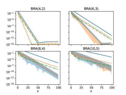
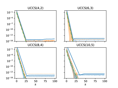
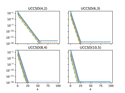
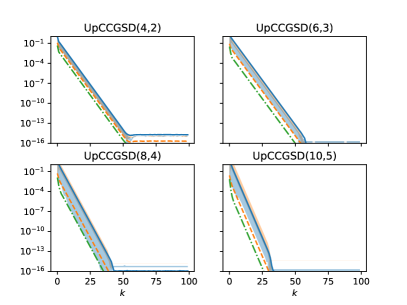
In Figure1 we plot the following quantities against different values of
, , and :
(1)the
distance between and ;
(2)the distance (relative error) between cost variance
at and , with respect to monomial observables
and .
All these distances converges to 0 as increases until exhausting machine
precision, validating our predictions.
Moreover, it appears that all these distances decays at least as
for some .
Based on this discovery, we made the following conjecture.
Figure 1:
Convergence of the projected state and cost variance with respect to .
For different ansatzs -BRA, -UCCS, -UCCSD and -UpCCGSD, and
different , we compare the
distance between
and
, and the relative difference between cost
variance at and the predicted asymptotic variance for all one- or
two-electron terms.
Notice that the cost variance is bounded by the distance multiplied by
the norm of the observable.
The logarithm of distance in all cases decreases almost perfectly in a linear
manner as increases, until reaching the machine precision.
Conjecture.
For any electronic structure Hamiltonian with , there exists some , such
that
(16)
Here is the cost function that implicitly depends on .
Moreover, for -BRA, for -UCC(G)S,
for -UCC(G)SD and -UpCCGSD.
Summary and discussion.—
In this work, we conducted a rigorous analysis of cost concentration for the
alternated dUCC ansatz in the infinite depth limit.
Contrary to previous belief [34], we showed that the
chemically inspired ansatz can also suffer from BP.
It is worth noting that our work does not rule out the practicality of
chemically inspired ansatzs.
Firstly, our study focused on alternated dUCC ansatzs, while the trainability
of Trotterized UCCSD and adaptive variants [35] remains
open.
Secondly, the BP phenomenon is considered under random parameter
initialization, whereas VQE typically benefits from reasonable heuristics for
choosing an initial guess.
BP imply that the optimizer cannot escape local minimas, but there is still a
possibility that the initial guess is already inside the same narrow gorge as
the optimal solution.
Lastly, we exclusively considered the Jordan-Wigner transformation, as employed
in the canonical implementation of UCCSD.
However, results in [18] suggest that the Bravyi-Kitaev
transformation might be a better choice due to its locality.
Acknowledgements.
We thank Kecheng Liu for helpful discussions.
This work was supported in part by the National Natural Science Foundation of
China Grants No.62325210, 62272441, 12204489, 62301531, and the
Strategic Priority Research Program of Chinese Academy of Sciences Grant
No.XDB28000000.
Appendix
Throughout the text, we will use for Pauli matrices, for identity matrix, and for identity matrix.
Two additional matrices are used: qubit annihilation operator
, and occupation number operator .
The symbol is reserved for the number of orbitals (qubits), and for
the number of occupied orbitals.
For any matrix (for example ), we define
, where and
.
We use to denote the complex conjugate of , and to
denote the conjugate transpose of matrix .
represents the imaginary unit.
Denote the symmetric group on a set of size .
The set of bit string of length is denoted by .
For a bit string ,
denotes the flip of , i.e., and .
For two bit strings ,
denotes the bitwise dot, defined by
.
Appendix A Definitions and main results
In this work we study the scalability of various alternated disentangled
UCC (dUCC) ansatzs, which can be viewed as a relaxed version of Trotterized
UCC.
Recall that in UCC theory, the trial wave function is parameterized as the
unitary exponentiation of excitation operators acting upon a reference state :
(17)
Here we use the convention that () label the occupied
(virtual) orbitals, but generalized excitations without the occupation
constraint are also allowed (and we will use for all orbitals
to emphasize the difference).
The widely used UCCSD variant corresponds to truncated up to second
excitations.
For circuit implementation, it is unclear how to exactly implement the large
exponentiation in Eq.17 efficiently (i.e., to polynomial number of one
and two qubits gates), except for the case when there are only single
excitations.
The canonical approach is to take a th order Trotter approximation, with
systematic error up to .
In contrast, for the ease of our analysis, we will incorporate an additional
relaxation step after Trotterization, as described below:
(18)
where
.
Remark that and are different set of parameters,
and we implicitly make the assumption that all parameters are real (this is
valid if we only care about real wave functions).
Obviously, such relaxation can offer higher variational accuracy, at the cost
of higher training overhead.
We refer to the last unitary in Eq.18 as alternated dUCC
ansatz111The term “dUCC” was coined in [13],
where it was used to refer to any sequence of excitation rotations (similar to
an 1-step Trotterization but conceptually different), and was proved to be able
to express the exact FCI state in the limit even when only single
and double excitations are involved.
We add the “alternated” prefix to emphasize the alternative structure.
, which
is formally defined below.
To avoid bothering with the fermionic ladder operators , we will identify with respectively, by Jordan-Wigner
transformation222Jordan-Wigner transformation is also employed in the
canonical implementation.
Other transformation such as Bravyi-Kitaev’s may be investigated in future
work.
.
A “qubit” version of UCC theory, where the -string is eliminated after
Jordan-Wigner transformation, is also considered in this work.
Definition A.1(Alternated (qubit) dUCC ansatz).
Call the unitary () an
alternated (qubit) dUCC ansatz, if it can be written as
(19)
where is a sequence of (qubit)
excitation rotations,
and
(or
in
qubit version).
While DefinitionA.1 encompasses any (qubit) excitations, our primary focus
lies on single and double (qubit) excitations.
This is particularly relevant in scenarios like UCCSD.
To this end, we will introduce dedicated notation for single and double (qubit)
excitation rotations, as follows.
(20)
(21)
where “h.c.” stands for Hermitian conjugation, and .
Examples of alternated (qubit) dUCC ansatzs (including at most double (qubit)
excitations) are
(22)
(23)
(24)
(25)
(26)
(27)
(28)
(29)
(30)
(31)
In VQE, the cost function to be optimized is naturally chosen to be
energy of the molecule system:
(32)
Here
•
is an easy-to-prepare reference state.
In this work, is fixed to be , where is a
Hartree-Fock state,
(33)
•
is the ansatz, such that
produces a trial state.
•
is the observable, usually the electronic structure Hamiltonian
.
In our study, we focus on the real case, where the one- and two-electron
integrals and are assumed to be both real and symmetric
( and ).
Moreover, we assume that only if or .
In other words, terms such as are forbidden.
It is important to note that this assumption is made for ease of analysis,
rather than due to the drawback of our proof techniques.
In fact, our results can be generalized to any observables, although the
progress of extending the analysis could be tedious.
Remark that under the aforementioned assumptions, can be
written as:
(34)
The cost function we study may take various forms, with
fixed, and potentially varying in different instances.
For simplicity, we will slightly abuse the notation and use
or even
instead of , whenever the context
is clear.
While VQA and VQE are promising in NISQ era, there are several unresolved
obstacles, among which the Barren Plateaus (BP) phenomenon poses a major
concern [34].
Analogous to the gradient vanishing problem in training classical neural
network, BP refers to the exponential concentration of gradients (of cost
function in VQA) around 0 over random parameters, thus ruling out any gradient
based optimization method with random starting point.
Another related concept is the concentration of cost function, which also
characterize the flatness of cost landscape.
For example, the exponential concentration of cost function around its mean
would rule out any gradient-free optimization method with random starting
point.
The two types of concentration are strictly defined as follows.
Let be a family of cost functions indexed by
qubit number and
for all .
Definition A.2(Gradient concentration and BP).
Let .
We say the gradients of concentrate polynomially
if , and concentrate exponentially if
.
Specifically, exhibits BP if the gradients
concentrate exponentially.
Definition A.3(Cost concentration).
Let .
We say concentrate polynomially if
, and concentrate exponentially if
.
Intuitively, both gradient concentration and cost concentration describe the
flatness of landscape.
In [30], the equivalence between exponential cost
concentration and exponential gradient concentration (i.e., BP) was established
for ansatzs comprising a polynomial number of independent Pauli rotations,
using integral arguments and the parameter shift rule.
Since their result is not directly applicable in our setting, in the following
lemma we derive a quantitative relationship between cost variance and gradient
variances, using the fact that the cost function of alternated dUCC ansatz is
periodic and has no rapid oscillations.
The proof of this lemma is postponed to AppendixB, and is largely
inspired by [28].
Lemma A.4(Relationship between variances of cost and gradients).
Let be an alternated (qubit) dUCC ansatz
defined in Eq.19, and defined in
Eq.34, then
(35)
Consequently, for alternated dUCC ansatzs, the exponential decay of cost
variance implies exponential decay of gradient variance by second inequality of
Eq.35, while the reverse holds only when is
sub-exponential by the first inequality.
Our main focus will be determining the scaling of variance of cost, and bound
the variance of gradients by LemmaA.4.
We prove in our main result (TheoremA.5) that while variants of alternated
(qubit) dUCC ansatz (-UCCSD, -BRA, etc.) differs both in structure and
performance, their asymptotic behavior of cost variance in the large depth
limit can be categorized by a few representatives.
Theorem A.5(Main result).
Let be an alternated (qubit) dUCC ansatz
defined in Eq.19, and
defined in Eq.32,
where the qubit number is , and defined in Eq.34,
with .
Denote the simple undirected graph formed by index pairs of (qubit) single
excitations in by , i.e.,
(36)
Suppose is connected.
The limit exists, and
1.
If contains only single excitation rotations, then
.
2.
If contains only single qubit excitation rotations, then if the maximum degree of is 2, and otherwise.
3.
If contains both single and double excitation rotations, then .
4.
If contains both single and double qubit excitation rotations (and
satisfy the condition in TheoremH.2), then .
AppendixesC to H are devoted to the proof of TheoremA.5,
which is in fact the calculation of cost variance .
The proof is divided into the following parts (illustrated in Figure2):
•
In AppendixC, we give a high
level description about how we calculate the th moment of cost function.
–
We represent the th moment of cost function as a circuit-like tensor
network (LemmaC.1), by contracting initial state, gates and observable into larger
tensors: .
Since the th moment of cost is essentially captured by the vector
, we refer to such vector as
-moment vector (DefinitionC.2).
–
We introduce site decomposition (DefinitionC.3), so that the enlarged space
involved in calculating can be still viewed
as tensor product of subsystems.
These subsystems are referred to as sites, each containing qubits.
Under site decomposition, tensor like can be viewed as an
operator acting on sites.
–
We show that each is an orthogonal projection (LemmaC.6), denoted
by .
–
The convergence of alternating projections hence assures that , where (CorollaryC.8).
While it is not obvious how to find the intersection space , it is easy to
find its orthogonal complement , since (LemmaC.9).
•
In AppendixD, we characterize the spanning set of (LemmaD.9).
Symmetries of is used to reduce the space.
–
The -symmetry helps to reduce to the invariant space
(CorollaryD.3).
–
The particle number symmetry helps to further reduce to the
invariant space
(LemmaD.8) when .
–
The -symmetry helps to reduce
to the invariant space (CorollaryD.13).
•
In AppendixE, we prove that the cost function is unbiased, i.e.,
the first moment is zero.
We also illustrate how to calculate the second moment by an example.
•
In AppendixesF, G and H, we prove our main result TheoremA.5,
by calculating , and taking the
inner product between and
which evaluates to .
–
The proof of case 1 and part of case 2 is constructive: we give an explicit
vector , and prove by showing that and .
In this proof, we use the spanning set of the orthogonal complement inside
—
.
–
We prove the rest of the theorem by showing that .
In such case, is obvious.
Figure 2:
Illustration of how we calculate the th moment of cost function.
(a) Tensor network representation of the th moment.
Here the square bracket represents taking the th moment.
(b) Use the independence of parameters to contract the tensor network into
a circuit-like one.
(c) The th moment of each excitation rotation is orthogonal projection.
In the infinite depth limit, these projections contract into an orthogonal
projection onto the intersection space .
(d) The th moment in the infinite depth limit can be recovered as
the inner product between vector and moment vector
(projected ).
In this section, we prove the equivalence between variances of cost and
gradients for alternated (qubit) dUCC ansatz (LemmaA.4).
In fact, we prove a more generalized version in LemmaB.2 for any
bounded frequency periodic function (defined below).
Intuitively, such function does not have rapid oscillation.
Definition B.1(Bounded frequency periodic function).
A function is called bounded frequency
periodic, if it is periodic with the following Fourier expansion
(37)
Moreover, there exists a constant independent of , s.t.
(38)
Notice that we implicitly assumed bounded frequency periodic function to have
period , but it can be generalized to any periodic function by rescaling.
The following proof is similar to Lemma 1 of [28].
We include the proof for completeness.
Lemma B.2(Relationship between variances of cost and gradients, generalized).
For bounded frequency periodic function where
the frequencies are bounded by as in Eq.38,
(39)
Proof.
Expand in Fourier basis as in Eq.37.
Since is real-valued, for any .
Since for any integer , we
have
(40)
(41)
By the fact that ,
(42)
∎
The following two lemmas show that the cost function of alternated (qubit) dUCC
ansatz is bounded frequency periodic, completing the proof of LemmaA.4.
Lemma B.3(Periodicity of (qubit) excitation rotations).
Let be a (qubit) excitation rotation (DefinitionA.1).
is periodic with period .
Moreover, there exists constant matrices , such that
(43)
Proof.
Recall , where
.
Notice that is anti-Hermitian.
It suffices to show that the eigenvalues of are
.
In fact,
(44)
Hence, is a diagonal matrix,
and each element on the diagonal is either 0 or -1.
∎
Lemma B.4.
Let be an alternated (qubit) dUCC ansatz
defined in Eq.19.
The cost function defined in Eq.32
is bounded frequency periodic.
To conclude this section, we make two remarks.
First, the lower bound in LemmaB.2 can be saturated, for example by the
function .
Notice that emerges as the global cost function
, where and
.
Second, we only utilize the periodicity of alternated (qubit) dUCC ansatzs
(LemmaB.3) when proving the equivalence between cost variance and
gradient variance.
Such argument could possibly be strengthened using other properties such as
non-locality.
Appendix C Moments of cost function
In the last section, we showed that for alternated dUCC ansatzs, the variance
of gradient can be bounded by the variance of cost itself in both directions
(LemmasB.2 and B.4).
For now on, we turn to calculate to the variance of cost function.
To start with, we employ the common trick in the study of BP
[22, 23, 24, 25]
to express the th moment of cost function as a circuit-like tensor
network.
The motivation is to separate initial state, gates and observables apart, and
to resolve the non-linearity in high order moment.
C.1 Circuit-like tensor network representation of
and moment vector
In this section, we express the th moment of cost function as a
circuit-like tensor network.
All quantum gates related to the same parameter are contracted to one
“elevated” tensor which has a larger dimension, namely, the th moment
superoperator.
The (matrix form of) thmoment superoperator of an operator with a real parameter is defined to be
(48)
To simplify the notations, we will use the shorthand
whenever the context is
clear.
Moreover, we introduce dedicated notation for the 1st
and 2nd moment of , since they will be used frequently:
(49)
The vectorization of an operator is
defined to be .
Using the fact that for independent random variables ,
we can express the th moment of cost function of alternated (qubit) dUCC
ansatzs by the product of th moment of excitation operators.
Lemma C.1(th moment of cost function).
Let be an alternated (qubit) dUCC ansatz
defined in Eq.19, be the cost
function defined in Eq.32 where is any observable.
For any and observables ,
(50)
In particular, the th moment of cost function for some observable is
(51)
Proof.
Observe that , and use the independence of parameters.
∎
Eq.50 is useful in calculating covariance, or other quantities alike.
2.
The expectations in LemmaC.1 are taken over random
parameters sampled from , or
equivalently from by the periodicity of (qubit)
excitation rotations (LemmaB.3).
LemmaC.1 indicates that the th moment of cost function for
different observables are essentially captured by a vector, which is the
product of th moment superoperators of excitation rotations and initial
state.
In other words, one can in principle calculate for
any observable if such vector is known — just take an inner product of
the vectorization of and the vector.
Hence, we refer to such vector as a moment vector, as defined below.
Definition C.2(-moment vector).
Let be a sequence of excitation rotations defined in DefinitionA.1,
and be the Hartree-Fock state defined in Eq.33.
For , the -moment vector is defined
to be
(52)
In particular, the moment vector of -UCCSD, -BRA etc. is denoted by
etc. And
the moment vector of -qubit-UCCSD etc. is denoted by
etc.
C.2 Site decomposition: a straightforward way to describe the elevated
tensors
So far, we have addressed the non-linearity in calculating the th moment
of cost by considering replicas of the original system.
Moreover, turns out to be the inner product of the vectorization of
and the -moment vector .
Before delving into the calculation of , it is
worthwhile to reorder the qubits in the enlarged Hilbert space so that the
elevated tensor can be described naturally.
Such reordering, which we refer to as site decomposition, is formally
defined below.
Definition C.3(Site decomposition).
The isomorphism between Hilbert spaces with , defined by
(53)
is
called a site decomposition.
Each is called a site of length
.
Moreover, we will use to denote any state in the enlarged space
, while is reserved for computational basis
states.
is interpreted as a bit string in .
For , denotes the bit string of the th
site, and denotes the th bit of th site.
This procedure described in DefinitionC.3 can be understood as reordering and
splitting the qubits into equally-sized subsystems, with each
subsystem forming a site.
As an example, the th moment of a qubit single excitation rotation
acting on qubit 1 and 2 can be viewed as a tensor acting on site 1 and 2, as
illustrated in Figure3.
Without site decomposition, it is less straightforward to describe such tensor.
Figure 3:
Illustration of the th moment of a double qubit gate acting on qubit
1 and 2, which can be viewed as a larger tensor acting on site 1 and 2.
Here and .
Each ball represents a qubit, the gray boxes together represent the th
moment of the double qubit gate, and the balls in the red dashed cycle form the
3rd site of length .
The reader should be aware that we will implicitly assume site decomposition in
the subsequent text.
The following proposition reexpress the initial state and vectorization of
observable and
under site decomposition.
Proposition C.4(Initial state and observable under site decomposition).
Let , and as defined in Eq.33.
Under site decomposition,
(54)
After Jordan-Wigner transformation, when (),
(55)
And when (),
(56)
Proof.
Notice that after Jordan-Wigner transformation , and the vectorization of is , respectively.
∎
The following operators related to sites will be useful.
Definition C.5().
Let .
1.
Define to be the permutation
of sites by :
(57)
In particular, denote the swap of site and .
2.
Define to be the permutation
of qubits in one site by :
(58)
3.
Define to be the flip of
the th bit in the th site for all :
(59)
In particular, denote .
C.3 Moments of excitation rotations
After introducing site decomposition, we now return to the calculation of
moment vector .
Recall the definition of in DefinitionC.2.
Since the initial state is fixed to be , it remains to determine
each , where is some (qubit) excitation rotation.
The following lemma give some basic properties of .
More properties will be covered in later sections.
Lemma C.6(Basic properties of ).
Let be a (qubit) excitation rotation (DefinitionA.1), and
.
1.
.
2.
is an orthogonal projection.
3.
Suppose is a qubit excitation rotation, i.e., for some
.
Define , and
(60)
Then
(61)
Here we use the convention that ,
and is the union of the following cases:
•
for some .
•
and for some .
•
One of and is odd.
4.
Suppose is an excitation rotation, i.e., for some .
Assume for index set .
Define and .
The following conversion rule holds:
One of the most important finding in LemmaC.6 is that the th
moment superoperator of (qubit) excitation rotations are
orthogonal projections.
This is not unusual in BP studies.
For example, in [15, 18, 24] the
circuit (or block of gates) is assumed to be Haar random up to 2nd moment.
Under such assumption one verifies that the 2nd moment superoperator of the
circuit (or block of gates) is an orthogonal projector of rank 2.
However, the projectors we encountered is significantly more complex compared
to the Haar random case.
In fact, the 2nd moment of qubit single excitation rotations is a projector
of rank 70 in the subsystem it acts on, let alone normal excitation rotations
which are highly non-local.
Hence, we do not expect it to be easy to figure out or even bound
for any finite .
Rather, we turn to study the infinite- case, which turns out to be
tractable.
The phenomenon that infinite case is easier than finite one is ubiquitous, for
example in the theoretical analysis of classical neural networks
[32].
The following lemma will play a central role.
Lemma C.7(Convergence of alternating projections [31]).
Let be a Hilbert space, and denote to be the orthogonal
projection onto a subspace .
Given subspace with intersection ,
(70)
Remark that we are working in a finite Hilbert space, and in such case uniform
convergence can
be shown.
Corollary C.8.
Let be a sequence of excitation rotations defined in DefinitionA.1,
and .
Denote the projection by , where is the subspace
that projects onto.
Define .
We have
The reason why the infinite case is easier is that by CorollaryC.8
it suffices to figure out the intersection , rather
than tracking how evolves.
2.
In the subsequent text, regardless of the form of and order of
moment , we will denote the subspace that projects
onto by , and the intersection space by , as in CorollaryC.8.
The reader should be cautious with which and is used in context
to define and .
While we may be able to characterize (albeit a bit complex) each , since
the matrix form of has been explicitly written out in
LemmaC.6, it is not obvious how to calculate their intersection at first
sight.
On the other hand, it is straightforward to determine the spanning set of the
orthogonal complement if one has determined the spanning set of
each — just take the union of these spanning sets.
The reason is explained in LemmaC.9 (2).
LemmaC.9 also includes other properties of orthogonal complement which will be
used in later sections.
The proof of LemmaC.9 is elementary and is omitted.
Lemma C.9.
Let and be subspaces of finite dimensional vector
space .
1.
.
2.
.
3.
.
4.
.
If in addition for all , then
5.
.
6.
Appendix D Reduce the space by symmetries
In the last section, we have hinted how we will calculate the th moment
of cost function at for alternated dUCC ansatzs:
1.
we find out the spanning set of each
(recall that ),
2.
take the union to
get the spanning set of (recall that ),
3.
somehow calculate , using the
spanning set of ,
4.
finally take the inner
product between and
, which
evaluates to .
Step 2 and 4 has been explained in the last section.
This section will be devoted to step 1, and will sketch the idea
behind 3.
We do so by restricting ourselves into invariant subspaces using symmetries of
.
The reduction of space is in sequence.
It is worth noting that while these symmetries should apply for any (qubit)
excitation rotations and any , we primarily focus on the
cases of (qubit) single/double excitation rotations and , since these
are enough for proving TheoremA.5.
D.1 -symmetry
The -symmetry of helps to reduce from the
whole space to , the
space spanned by states where each site has an even Hamming weight.
Definition D.1().
Define as follows:
(72)
Let be a (qubit) excitation rotation, and be a sequence
of (qubit) excitation rotations (DefinitionA.1).
Lemma D.2(-symmetry).
For any , .
Proof.
Notice that for some
(qubit) excitation , and either commutes or anti-commutes
with (since commutes with and
anti-commutes with ).
•
If commutes with , then commutes
with , and thus commutes with .
•
If anti-commutes with , then .
∎
Corollary D.3(Invariance of ).
is an invariant subspace of .
Moreover,
.
Proof.
Notice that is the common +1 eigenspace of
.
Since and
commute mutually, is an
invariant subspace of .
By PropositionC.4, .
Hence,
.
Since is closed,
.
∎
The invariance of is enough to calculate the
first moment of cost function.
The reader can jump to AppendixE for more details.
In order to calculate the second moments, however, we still need to find the
spanning set of , or equivalently diagonalizing
.
Since is an invariant subspace that contains
, we can diagonalize inside
to save some work.
But before that, we first introduce special notations for sites with an even
Hamming weight at , so that the notation for states in
can be simpler.
Recall that when , each site has a length of , indicating that the
dimension of the Hilbert space for each site is .
Out of the 16 computational basis states of each site, there are 8 with an even
Hamming weight, as follows.
Definition D.4(8 special basis states of site at ).
Define 8 product state in as follows:
(73)
Namely, they are
(74)
(75)
Remark that
.
For example, the following state is a paired state at .
Different “pair”s are marked in different colors.
(76)
We can give the square of the vectorization of and
a more succinct expression compared to that in PropositionC.4,
using the notations as follows.
Proposition D.5(Succinct expression of ).
After Jordan-Wigner transformation, when (),
(77)
And when (),
(78)
Now that we have defined the notation , we return to
the diagonalization of inside .
The following lemma gives diagonalization of and
partial diagonalization of inside
.
These will be used in the next section to derive the spanning set of
for .
Lemma D.6(Diagonalization of inside ).
1.
The subspace that
projects
onto is spanned by , where
(79)
(80)
(81)
2.
The space spanned by is invariant under ,
and when restricted in such subspace, is an
orthogonal projection onto the space spanned by .
Proof.
1. —
By LemmaC.6 (3), stabilizes
every vector in , and
(82)
Finally, since are mutually orthogonal,
is a
projection onto .
Thus, is invariant under , and
is indeed an
orthogonal projection onto the space spanned by .
∎
D.2 Particle number symmetry
The particle number symmetry of helps to reduce the
space from to
, where certain constraints regarding the
number of must be satisfied.
Notice that we exclusively focus on the case for particle number
symmetry, but such symmetry should hold for general .
Definition D.7(Paired state and related notions).
Let and .
1.
For any , define
(84)
If is omitted, it is assumed that , i.e.,
.
2.
Call a paired state, if
(85)
(86)
3.
Denote the set of all paired states by , and
the Hilbert space spanned by these states by
.
4.
Define the configuration of a paired state by
(87)
5.
Denote the set of all paired states with configuration by
, and the Hilbert space spanned by
these states by .
Remark that the 8 numbers is
uniquely determined by the configuration of a paired state , and
.
Lemma D.8(Invariance of ).
Let be a sequence of (qubit) excitation rotations, with .
is an invariant subspace of each
.
Moreover,
.
Proof.
In order to prove invariance of , it
suffices to show that
, for all
and
.
•
We first prove the case when .
Since (and )
acts non-trivially only on 2 (and 4) sites, one can enumerate (and )
states of these sites to verify that if has non-zero overlap with , then for
all and ,
(88)
Thus, .
In fact, Eq.88 is obvious when by the
diagonalization given in LemmaD.6 (1).
•
In order to prove the case when , we utilize the conversion rule
in LemmaC.6 (4).
Notice that for any and , there exists
and , such that for any ,
(89)
Here is defined as in LemmaC.6
(4) with respect to .
Thus, if has a non-zero
overlap with , then
Finally, by PropositionC.4, .
Hence,
.
Since is closed,
.
∎
LemmaD.8 indicates that we can restrict ourselves in
— instead of the spanning set of each
, it suffices to find the spanning set of the orthogonal
complement of each inside :
.
As one may expect, the union of these spanning set spans , according to LemmaC.9
(4).
The following lemma characterizes the spanning set of for .
Lemma D.9(Spanning set of for
).
Denote by the space that projects onto.
Suppose for (qubit) single excitations and for (qubit)
double excitations.
1.
is spanned by all the following
vectors: for any ,
let ,
•
.
•
if .
2.
is spanned by all the following
vectors: for any ,
•
.
•
if .
3.
contains , where , , and .
4.
contains , where , and .
Proof.
We first prove 2 and 4 using diagonalization of
in
(LemmaD.6), then prove
1 and 3 using the qubit to non-qubit conversion rule in
LemmaC.6 (4).
2. —
Denote the set of specified vectors by .
Obviously, .
We need to prove (1) , (2) (since that would imply ).
(1)
: We
show that every vector in is orthogonal to
defined in LemmaD.6 (1), hence .
First, consider the vector .
•
If , then and is
orthogonal to .
•
If , then is orthogonal
to . is also orthogonal to
since while for vectors
in the overlaps with and
are the same.
•
Otherwise, is orthogonal to .
is also orthogonal to since for vectors in the
overlaps with and differ by
.
Next, consider the vector with .
is orthogonal to .
is also orthogonal to since for vectors in the overlap
with equals one of the overlaps with , while the rest two are both
zero.
(2)
: Suppose , we prove .
Write , with .
Since is orthogonal to , we have
•
if .
•
if and .
Hence,
(93)
It is straightforward to verify that
and by LemmaD.6 (1) .
Thus, .
4. —
Obviously, .
Use the notation from LemmaD.6 (2).
Since is an invariant space of and
, we have .
is orthogonal to since .
is also orthogonal to , since for vectors in the overlaps with and differ by .
Hence, by LemmaC.9 (5).
1 and 3. —
Same as 2 and 4 but use the conversion rule.
∎
LemmaD.9 has a simple yet interesting corollary —
if contains enough (qubit) single excitations, the dimension of
is at most .
Moreover, vectors in has a nice
decomposition which we refer to as decomposition in configuration basis.
Let be a sequence of (qubit) excitation rotations defined in
DefinitionA.1, be the intersection space defined in LemmaC.7.
Denote the simple undirected graph formed by index pairs of (qubit) single
excitations in by as in TheoremA.5.
If is connected, then there exists a function
which defines a set of
configuration basis , such that for any
,
(94)
Proof.
By LemmaD.9, , for any
and .
By LemmaC.9, .
Hence, for any , we have
.
In other words, if two paired states differ only by a site swap on an edge,
their overlaps with differs by either or , and such
relative sign is independent of .
Since is connected, one can argue that if two paired states
has the same configuration , their overlaps
with differs by at most — two paired states with the
same configuration differ by some site permutation, which can be decomposed
into product of swaps, and each swap can in turn be decomposed into product of
swaps on edges.
The decomposition of a site permutation into swaps on edges may not be unique,
and if the signs induced by two different decomposition conflict, it must be
for all
(one can argue that , and thus
).
Otherwise, the relative signs for paired states in
must be unique, and are independent
of .
Hence, one can pick a sign function that satisfies the requirements — on
, define
arbitrarily, and otherwise define
arbitrarily on some ,
and extend to other
according the unique relative sign.
∎
Now that we have characterized the spanning set of , we are prepared to prove case 1 and part of
case 2 of TheoremA.5.
Our proof for these parts is constructive — we will give an explicit vector
, and prove that
.
To be precise, we show that the following two conditions holds:
The reader can jump to AppendixesF and G for more details.
Remark that such proof relies on the complete spanning set of .
We have only given an incomplete spanning set for of
, thus simply taking the
union of these spanning set is not enough.
In fact, to prove the rest of TheoremA.5 we utilize another symmetry
discussed in next section to reduce the space down to one dimension.
In such case is obvious.
D.3 -symmetry
The -symmetry of helps to further
reduce the space .
We use this symmetry to find a one-dimensional subspace of , which contains
.
Definition D.11().
For any , is defined to be
the +1 eigenspace of .
Let be a (qubit) excitation rotation, and be a sequence
of (qubit) excitation rotations (DefinitionA.1).
Lemma D.12(-symmetry).
For any , .
Proof.
, since the action of
induces a permutation of replicas of
by , which does not change the result.
∎
Corollary D.13(Invariance of ).
For any , is an invariant
subspace of .
Moreover,
.
We use the following lemma to reduce the space to dimension one in later
proofs.
Lemma D.14.
Let be a sequence of (qubit) excitation rotations.
Denote the simple undirected graph formed by index pairs of (qubit) single
excitations in by as in TheoremA.5.
Suppose
1.
is connected.
2.
For all where at
least two of is non-zero, .
Then,
(95)
where .
Proof.
Since is connected (1st condition), vectors in admits decomposition in configuration basis
(CorollaryD.10), say, with
.
Moreover, by the 2nd condition, if two of is non-zero.
We prove (1) , and likewise for
configuration and , (2) , (3) the coefficients
of in are exactly those
provided in Eq.95.
(1)
We prove that , for any (and similarly or ) and .
After that, one can argue in the same way as in CorollaryD.10 to complete the
proof.
Suppose .
By definition of , either or is contained
in .
•
If , by LemmaD.9
(2) .
Since , we have .
Hence, , and .
•
If , by LemmaD.9 (1) , where .
Since , we have .
Hence, .
The remainder is similar as the previous case.
(2)
Fix a vector .
We have proved that .
Denote by the coefficient of in , where at most one of is non-zero.
Define if at least two of is non-zero.
We prove that (2.1) , (2.2)
.
If so, it must be .
Hence, .
(2.1)
Fix .
Suppose .
We need to prove that is orthogonal to ,
since the configuration of is respectively,
and hence .
If two of are non-zero, then and the equality holds trivially.
Assume without loss of generality that .
Once more by definition of , either or is
contained in .
If , by LemmaD.9 (1) , where .
Since , we have .
Thus, , while .
By the 2nd condition, , since the configuration of is
and , and likewise for .
Hence, .
(2.2)
Fix a vector and
two swaps .
Let .
It is easy to check that the configuration of is respectively.
By DefinitionD.11, and .
Finally, since , we have and .
(3)
Since , there exists constant such that
.
Recall that , thus
(96)
Solving the equation one obtains the desired coefficients.
∎
Appendix E Average of cost is zero
In this section, we will prove that cost function of alternated dUCC ansatzs is
unbiased, i.e., , where
is an electronic structure Hamiltonian.
We also sketch a failed attack towards the variance of cost function, which
serves as an illustration of techniques used in the proof of main results.
Theorem E.1(Unbiased cost function).
Let be a cost function defined in
Eq.32, where is an alternated (qubit)
dUCC ansatz defined in Eq.19, and is an electronic structure
Hamiltonian defined in Eq.34.
We have .
As a corollary, to calculate the variance of cost, it suffices to calculate the
2nd moment, since
(98)
Now we sketch a failed attack towards the variance of cost.
The reader can safely skip this part.
It would be great if we can give a nontrivial bound of the 2nd moment of
cost function using only 1st moments, for example utilizing the following
inequality:
(99)
Unfortunately, it is not the case, at least not for Eq.99.
The derivation is sketched below, and may serve as an example of the techniques
used in the proof of main results.
Suppose we wish to bound by calculating
.
For simplicity, we consider the case , since it is straightforward to generalize to other cases.
We further assume that the index pairs of (qubit) single excitations in
form a connected graph, i.e., there exists a connected simple graph
, such that and contains (or
) for all .
The importance of this assumption would be made clear below.
Recall that (LemmaC.1 and DefinitionC.2).
Since
(PropositionC.4) and is invariant under
for all (CorollaryD.3), we can restrict ourselves in
the subspace .
Fix an , and suppose , where (or the corresponding qubit version).
By LemmaC.6 (3 and 4), for any ,
(100)
Notice that preserves the number of and
in , due to particle number symmetry.
In particular, if (or ) for any , and
differ by , the equality implies that .
The connectivity of and the particle number symmetry thus indicates
(101)
The coefficient in (Eq.101) must be by the
equality .
Lastly, since ,
(102)
And therefore,
(103)
Such upper bound is at least , and is roughly
when , definitely not enough to argue an exponential decay which is
a sufficient condition of BP.
Appendix F Proof of main result: Case 1
In this section we prove the polynomial concentration of cost function for
alternated dUCC ansatz containing only single excitation rotations, with mild
connectivity assumption (TheoremA.5 (1)).
Examples of such ansatzs include -BRA, -UCCS and -UCCGS.
Definition F.1(Crossing number of paired state).
Let .
Draw a graph of vertices according to as follows:
1.
Place the sites of in order on a
circle.
Color by red, by
green, and by blue.
Do not color .
2.
Draw an edge inside the circle between any two sites of the same
color, and color it with this same color.
Make sure no three edges cross at the same point.
The crossing number of , denoted by
, is defined to be the minimal number of
crossing points of edges in color red and green, or green and blue, or red and
blue.
Alternatively, suppose site is colored by as
above,
(104)
Figure 4:
Illustration of DefinitionF.1.
The crossing number of this paired state is 2, with the corresponding crossing
points marked by gray balls.
Notice that there are 3 crossing points not counted into the crossing number,
since the horizontal edge is not colored.
For example, the crossing number of the paired state in Eq.76 is 2
(Figure4).
We need the following properties of crossing numbers in the proof.
Lemma F.2(Properties of crossing numbers).
Let .
The following properties of crossing numbers holds.
1.
.
2.
If , then
(105)
Proof.
1. —
The key observation here is that by swapping two neighboring sites of
, the parity of crossing number will change by .
Indeed, if one of or is not colored or are both in
the same color, then , and swapping with will not change the crossing number.
And if and are in different colors, then , and swapping with will
change the parity of crossing number, since there are even-number of red, green
or blue sites and thus the degrees of and are both
odd.
Consider the paired state sequence where
and
If , then .
By changing to (or ),
site and will both be colored by red (or green, blue), and the number
of crossing points increased will be even.
Hence,
Finally, notice that .
Combined with Eqs.111 and 112 we have proved Eq.109.
∎
Lemma F.3.
Let be a connected graph with vertices.
Suppose contains a subsequence of single excitation rotations
.
Let be the intersection space of defined in CorollaryC.8 at
.
For any , .
Proof.
The proof is similar to that of CorollaryD.10, but more specific.
•
Suppose for some and .
By assumption, there exist some such that .
Thus, by LemmaD.9 (1), , where .
By LemmaC.9, .
And by LemmaF.2, .
Hence, .
•
Otherwise, for some .
The permutation can be decomposed into product of swaps, and by the fact
that is connected, each swap can in turn be decomposed into product of
swaps on edges (pick an arbitrary path connecting in , the swap can be decomposed into product of swaps along the path).
Hence, there exists and a sequence of edges
, such that .
Let , we have
and for .
By the previous case, for .
The sum of these vectors yields
, which is also a
member of .
∎
Theorem F.4.
Let be a connected graph with vertices, be a
sequence of single excitation rotations .
Define .
The -moment vector is
(113)
where .
Proof.
Denote the right-hand side of Eq.113 by .
Use the notations from CorollaryC.8.
Since , in
order to prove , it suffices
to prove that (1) and (2) .
(1)
Obviously, .
We prove that is orthogonal to , for each .
If so, we have by LemmaC.9.
Recall the spanning set of characterized in LemmaD.9
(1).
Suppose .
For any , let
.
We check the following two cases.
•
is orthogonal to .
In fact, the overlap between these two vectors is proportional to
,
which is 0 by LemmaF.2 (1).
•
is orthogonal to .
In fact, the overlap between these two vectors is proportional to
(114)
Here we define .
By LemmaF.2 (2), the numerators in the four fractions in
Eq.114 are the same.
Factoring out the four identical numerators, it can be proved that
Eq.114 equals 0 for any integer using combinatorial arguments.
(2)
Next, we prove ,
by expressing as a linear
combination of vectors in .
Recalls that the union of the spanning sets of each (characterized in LemmaD.9
(1)) spans .
Here the under script indicates that the summation is taken over vectors in
Eqs.115 and 116.
Let .
Let be the number of different paired states with configuration :
(118)
and define
(119)
where
(120)
Comparing the coefficients of vectors in both sides of Eq.117, we have
to prove the following linear equations.
(121)
(122)
Here we define , and if at least one of
.
Eq.121 follows from definition.
It can be verified that the right-hand side of Eq.122 equals
(123)
which equals the left-hand side by definition.
∎
Notice that the moment vector in
TheoremF.4 does not depend on the structure of except the
connectivity.
As an immediate corollary, the -moment vectors of -BRA,
-UCCS and -UCCGS are the same, since the underlying graphs , which are
a path, a complete bipartite graph and a complete graph respectively, are all
connected.
With characterized, we can calculate the
2nd moment of cost function for any observables in the limit.
The case 1 of main result is stated formally as following corollary.
Corollary F.6(Main result, Case 1).
Let be defined in TheoremF.4,
be the cost function defined
in Eq.32.
Here the observable is an electronic structure Hamiltonian
defined in Eq.34, with coefficients .
We have
(125)
Proof.
Recall that
(126)
The contribution of cross terms is zero.
To see that, take
with
() as an example.
Notice that is the orthogonal projection onto
.
However,
(127)
Hence, .
Consequently,
since
.
The same argument can be extended to when one of or both are
double excitation Hermitians, except for the tricky case where
are both double excitation Hermitians and the sets of indices are the same.
For example, when ,
may not be 0.
However, we have assumed that terms like
do not appear in to rule out the non-zero cases, since they
are not essential.
In this section we prove the polynomial/exponential concentration of cost
function for alternated dUCC ansatz containing only qubit single excitation
rotations, with mild connectivity assumption (TheoremA.5
(2)).
Examples of such ansatzs include -qubit-UCCS and -qubit-UCCGS.
Theorem G.1.
Let be a connected graph with vertices, be a
sequence of qubit single excitation rotations
.
Define .
Depending on structure of , the moment vector
admits the one of following forms.
1.
If is a path or a ring, then with and
for all .
2.
If , is bipartite, and both parts of have an even size (i.e.,
let be the unique partition of vertices such that both and
are independent sets, and are both even), then
can be written in the form of Eq.94,
with
As an immediate corollary, we can determine the -moment
vector of -qubit-UCCS and -qubit-UCCGS, where the underlying graph is
a complete bipartite graph and a complete graph, respectively.
With characterized, we can calculate the
2nd moment of cost function for any observables in the limit.
Case 2 of main result is stated formally as following corollary.
Corollary G.3(Main result, Case 2).
Let be defined in TheoremG.1, and
be the cost function defined
in Eq.32.
Here the observable is an electronic structure Hamiltonian
defined in Eq.34, with coefficients .
1.
If is a path or a ring, then is the same as in
CorollaryF.6.
2.
If , is bipartite, and both parts of have an even size, then,
(132)
Here we define if a proposition is true and otherwise.
3.
Otherwise,
(133)
Proof.
Similar to the proof of CorollaryF.6, it suffices to evaluate
for
and .
The basis rotation ansatz consists of single excitation rotations acting on
edges of a path which connects all neighboring qubits, i.e., .
When acting on two neighboring qubits, single excitations are equivalent to
qubit single excitations ().
Thus, when is a path connecting all neighboring qubits,
is exactly .
Suppose is an arbitrary path.
Fix one of the two corresponding permutations , such
that .
By examining the proof of TheoremF.4, it can be checked that the moment
vector remains unchanged if one replace the initial state by any paired state in
.
Thus,
(139)
To extend the conclusion to rings, it suffices to show the equality for the
“standard” ring, i.e., , and
argue for arbitrary rings similar to Eq.139.
Let .
It suffices to prove that .
If so, one can replace by without changing
.
Since can also be replaced by for
, one concludes that according to TheoremF.4.
Equivalently, we prove that the spanning sets are the same for and .
By comparing 1 and 2 in LemmaD.9, we need to
prove for any with , that (1) , (2) if
, then .
Let be defined in TheoremG.1 (2).
Suppose is an edge of .
For any , if
, then .
Proof.
Let .
Recall that is a bipartite graph, and the two parts of
are both even.
Assume without loss of generality that .
By definition, .
We prove by comparing and .
•
If or , then
.
Hence, .
Meanwhile, .
•
If one of is or , then by the
definition of , at most one of is non-zero.
In such case, we have for any
.
Hence, .
Meanwhile, .
•
Otherwise, it must the case that exactly two of is non-zero,
and .
We have , since must be one of , by the fact is even.
Meanwhile, .
∎
Lemma G.5.
Let be defined in TheoremG.1 (2).
Suppose is an edge of .
For any , with
, let
.
We have
(141)
Proof.
We prove by evaluating the values of and in
Eq.141.
•
If , the signs of are all 1 and Eq.141
follows from the equality .
•
If exactly one of is non-zero, and ,
the signs of are all 1 and Eq.141 follows from the
equality .
•
If exactly one of is non-zero, and ,
the signs of are all 1.
To see that, we may assume without loss of generality that and
, and .
By definition, , and
(142)
since and for , and
is even.
Similarly, .
Eq.141 follows from the equality
(143)
•
Otherwise, we may assume that exactly two of is non-zero,
and , since in other cases the coefficients of
are all zero.
Assume without loss of generality that , and .
By definition,
(144)
since , , for ,
and is even.
Eq.141 follows from the equality
(145)
∎
Lemma G.6.
Let be a simple, connected graph with vertices and
.
Suppose contains a subsequence of qubit single excitation rotations
.
Let be the intersection space of defined in CorollaryC.8 at
.
For any , if one of
the following two cases happens, then .
1.
Two of are non-zero and .
2.
All of are non-zero.
Proof.
Fix a vertex such that , and pick from the neighborhood of .
Then form a star motif centered at .
(1)
Assume without loss of generality that .
Since , there is at least one or
in .
We may assume that
(146)
This is because by CorollaryD.10, once we prove ,
we can argue that for any .
Consider the vector sequence , and
(147)
(148)
It can be verified that .
By LemmaD.9 (2), the following vectors lie in .
(149)
(150)
Combining these vectors to eliminate , we get , since
.
(2)
Similarly assume that
(151)
Consider the vector sequence in Eqs.147 and 148.
By LemmaD.9 (2), the following vectors lie in .
(152)
(153)
Combining these vectors to eliminate , we get , since
.
∎
Lemma G.7.
Same condition as TheoremG.1 (2).
For , if
, then
.
Proof.
Suppose .
If satisfies the conditions in LemmaG.6, then
, hence .
Otherwise, by definition in Eq.130.
The rest of the proof is similar to that of LemmaF.3, using
LemmaD.9 (2), LemmaG.4 and connectivity of .
∎
Lemma G.8.
Same condition as TheoremG.1 (2).
For any , if one of the following
3 cases happens, we have .
1.
and .
2.
and .
3.
and .
Proof.
We prove the first case, since the rest 2 cases are similar.
It suffices to prove that for any , if , then .
Furthermore, we may assume that there exists and such that
, since one can then use LemmaG.7 to argue for general cases.
By definition of , there exists such that .
By LemmaD.9 (2) and LemmaC.9, .
Since , we have
according to LemmaG.6.
Hence, .
It remains to show that , which has been proved in
Eq.144.
∎
Denote the state specified in Eqs.130 to 131 by .
Use the notations from CorollaryC.8.
We proceed similarly as in the proof of TheoremF.4 by showing that (1)
and (2) .
(1)
Obviously, .
We prove that is orthogonal to , for each .
If so, we have by LemmaC.9.
Recall the spanning set of characterized in LemmaD.9
(2).
Suppose .
For any , we check
the following two cases.
•
is orthogonal to .
In fact, the overlap between these two vectors is proportional to
, which is 0 by
LemmaG.4.
•
is orthogonal to .
In fact, the overlap between these two vectors is proportional to
, which is 0 by
LemmaG.5.
(2)
Next, we prove ,
by expressing as a linear
combination of vectors in .
Recalls that the union of the spanning sets of each (characterized in LemmaD.9
(2)) spans .
And similarly by replacing (and the corresponding configurations), we
have
(160)
(161)
We prove that there exists functions , such that
(162)
Here the subscripts indicate that the summation is taken over vectors in
Eqs.154 to 161.
Abusing the notation in the proof of
TheoremF.4, we define .
is defined recursively as follows:
(163)
By comparing coefficients of vectors in both sides of Eq.162, we have
to prove the following linear equations:
(164)
(165)
(166)
(167)
(168)
(169)
Notice that Eqs.164, 165, 166 and 168 holds by definition, and one
can check that Eq.169 also holds.
To prove Eq.167, we multiply on both sides of Eq.166 to
get
It suffices to prove that if and at least two of is non-zero, then
.
The rest follows immediately from LemmaD.14.
Since we did not fall into case 1 or 2, it must be , and
(1)
,
(2)
or
contains an odd ring as subgraph, and the size of the ring is smaller than ,
(3)
or is bipartite, but one part of has an odd size.
We prove that in the first 2 cases, and in the 3rd case.
It suffices to prove the case where exactly two of are non-zero and , since otherwise according to
LemmaG.6.
Assume without loss of generality that and .
Suppose contains a ring as subgraph, where , and
is an odd number.
Assume without loss of generality that .
Consider the vector sequence where such that
(172)
It is easy to see that .
Construct a vector
for each according to LemmaD.9 (2),
one can argue that .
(3)
Suppose the two parts of are , and is odd.
We first show that for any , if and
, then
(173)
Here we define .
The proof is similar to LemmaG.7 and LemmaG.8, hence we only
provide a proof sketch.
•
Eq.173 holds if . —
For any edge , there exists such that .
By LemmaD.9 (2) and LemmaC.9, we have .
On the other hand, one checks that .
Hence, Eq.173 holds if .
The connectivity of then implies that Eq.173 holds if
.
•
Eq.173 holds if . —
We may assume that there exists and such that .
By LemmaD.9 (2) and LemmaC.9, we have .
By LemmaG.6, .
Hence, .
On the other hand, .
Hence, Eq.173 holds.
Remark that when is even, coincides with
defined in Eq.131, while when is odd
is always -1.
Next, we show that with , which
completes the proof.
Let .
It is straightforward to check that and .
Hence, by Eq.173 we have .
On the other hand, by definition of we have
.
Thus, .
∎
Appendix H Proof of main result: Case 3 and 4
In this section we prove the exponential concentration of cost function for
alternated dUCC ansatz containing both single and double (qubit) excitation
rotations, with mild connectivity assumption (TheoremA.5
(3 and 4)).
Examples of such ansatzs include -UCCSD and -UCCGSD, -UpCCGSD,
-qubit-UCCSD, -qubit-UCCGSD.
Theorem H.1.
Let be a connected graph with vertices, be a
sequence of single excitation rotations concatenated
with at least one double excitation rotation .
We have .
Proof.
It suffices to prove that if and at least two of is non-zero, then
.
The theorem then follows immediately from LemmaD.14.
Assume without loss of generality that , and
Combining Eqs.176, 177 and 178 to eliminate we get , since .
∎
For alternated qubit dUCC ansatzs, we make mild assumption about the topology
as well as the position of qubit double excitation rotations.
Theorem H.2.
Let be a connected graph with vertices and , be a sequence of qubit single excitation rotations
concatenated with at least one qubit
double excitation rotation .
Assume, only when and is a bipartite graph with two non-empty even
parts , that .
We have .
Proof.
If or is not a bipartite graph with two non-empty even parts,
then (TheoremG.1 (3)), and it must be
.
Otherwise, we show that if and at least two of is non-zero, then
.
The theorem then follows immediately from LemmaD.14.
Similar to the proof of TheoremH.1, we assume Eq.174, and consider
the paired state sequence Eq.175.
By LemmaD.9 (4),
Combining Eqs.179 and 180 to eliminate we get , since .
∎
As an immediate corollary, the moment vector of the 2nd moment at infinity
step of -UCCSD and -UCCGSD, -UpCCGSD, -qubit-UCCSD,
-qubit-UCCGSD are the same.
Corollary H.3.
We have
(181)
With moment vector of the 2nd moment characterized, we can calculate the
2nd moment of cost function for any observables.
Case 3 and 4 of main result is stated formally as following corollary.
Corollary H.4(Main result, Case 3 and 4).
Let be defined in TheoremsH.1 and H.2, and
be the cost function defined in
Eq.32 where is an electronic structure Hamiltonian
defined in
Eq.34.
is the same as CorollaryG.3 (3).
Notice that .
References
Peruzzo et al. [2014]A. Peruzzo, J. McClean, P. Shadbolt, M.-H. Yung, X.-Q. Zhou, P. J. Love, A. Aspuru-Guzik, and J. L. O’brien, A variational eigenvalue solver on a photonic quantum processor, Nature communications 5, 4213 (2014).
Kandala et al. [2017]A. Kandala, A. Mezzacapo, K. Temme, M. Takita, M. Brink, J. M. Chow, and J. M. Gambetta, Hardware-efficient variational quantum eigensolver for small molecules and quantum magnets, nature 549, 242 (2017).
O’Malley et al. [2016]P. J. O’Malley, R. Babbush, I. D. Kivlichan, J. Romero, J. R. McClean, R. Barends, J. Kelly, P. Roushan, A. Tranter, N. Ding, et al., Scalable quantum simulation of molecular energies, Physical Review X 6, 031007 (2016).
Nam et al. [2020]Y. Nam, J.-S. Chen, N. C. Pisenti, K. Wright, C. Delaney, D. Maslov, K. R. Brown, S. Allen, J. M. Amini, J. Apisdorf, et al., Ground-state energy estimation of the water molecule on a trapped-ion quantum computer, npj Quantum Information 6, 33 (2020).
Colless et al. [2018]J. I. Colless, V. V. Ramasesh, D. Dahlen, M. S. Blok, M. E. Kimchi-Schwartz, J. R. McClean, J. Carter, W. A. de Jong, and I. Siddiqi, Computation of molecular spectra on a quantum processor with an error-resilient algorithm, Physical Review X 8, 011021 (2018).
Fedorov et al. [2022]D. A. Fedorov, B. Peng, N. Govind, and Y. Alexeev, VQE method: a short survey and recent developments, Materials Theory 6, 1 (2022).
Barkoutsos et al. [2018]P. K. Barkoutsos, J. F. Gonthier, I. Sokolov, N. Moll, G. Salis, A. Fuhrer, M. Ganzhorn, D. J. Egger, M. Troyer, A. Mezzacapo, et al., Quantum algorithms for electronic structure calculations: Particle-hole hamiltonian and optimized wave-function expansions, Physical Review A 98, 022322 (2018).
Wecker et al. [2015]D. Wecker, M. B. Hastings, and M. Troyer, Progress towards practical quantum variational algorithms, Physical Review A 92, 042303 (2015).
Taube and Bartlett [2006]A. G. Taube and R. J. Bartlett, New perspectives on unitary coupled-cluster theory, International journal of quantum chemistry 106, 3393 (2006).
Lee et al. [2018]J. Lee, W. J. Huggins, M. Head-Gordon, and K. B. Whaley, Generalized unitary coupled cluster wave functions for quantum computation, Journal of chemical theory and computation 15, 311 (2018).
Dallaire-Demers et al. [2019]P.-L. Dallaire-Demers, J. Romero, L. Veis, S. Sim, and A. Aspuru-Guzik, Low-depth circuit ansatz for preparing correlated fermionic states on a quantum computer, Quantum Science and Technology 4, 045005 (2019).
Hatano and Suzuki [2005]N. Hatano and M. Suzuki, Finding exponential product formulas of higher orders, in Quantum annealing and other optimization methods (Springer, 2005) pp. 37–68.
Evangelista et al. [2019]F. A. Evangelista, G. K. Chan, and G. E. Scuseria, Exact parameterization of fermionic wave functions via unitary coupled cluster theory, The Journal of chemical physics 151 (2019).
Quantum et al. [2020]G. A. Quantum, Collaborators*†, F. Arute, K. Arya, R. Babbush, D. Bacon, J. C. Bardin, R. Barends, S. Boixo, M. Broughton, B. B. Buckley, et al., Hartree-fock on a superconducting qubit quantum computer, Science 369, 1084 (2020).
McClean et al. [2018]J. R. McClean, S. Boixo, V. N. Smelyanskiy, R. Babbush, and H. Neven, Barren plateaus in quantum neural network training landscapes, Nature communications 9, 4812 (2018).
Cerezo and Coles [2021]M. Cerezo and P. J. Coles, Higher order derivatives of quantum neural networks with barren plateaus, Quantum Science and Technology 6, 035006 (2021).
Arrasmith et al. [2021]A. Arrasmith, M. Cerezo, P. Czarnik, L. Cincio, and P. J. Coles, Effect of barren plateaus on gradient-free optimization, Quantum 5, 558 (2021).
Cerezo et al. [2021a]M. Cerezo, A. Sone, T. Volkoff, L. Cincio, and P. J. Coles, Cost function dependent barren plateaus in shallow parametrized quantum circuits, Nature communications 12, 1791 (2021a).
Marrero et al. [2021]C. O. Marrero, M. Kieferová, and N. Wiebe, Entanglement-induced barren plateaus, PRX Quantum 2, 040316 (2021).
Wang et al. [2021]S. Wang, E. Fontana, M. Cerezo, K. Sharma, A. Sone, L. Cincio, and P. J. Coles, Noise-induced barren plateaus in variational quantum algorithms, Nature communications 12, 6961 (2021).
Holmes et al. [2022]Z. Holmes, K. Sharma, M. Cerezo, and P. J. Coles, Connecting ansatz expressibility to gradient magnitudes and barren plateaus, PRX Quantum 3, 010313 (2022).
Pesah et al. [2021]A. Pesah, M. Cerezo, S. Wang, T. Volkoff, A. T. Sornborger, and P. J. Coles, Absence of barren plateaus in quantum convolutional neural networks, Physical Review X 11, 041011 (2021).
Zhao and Gao [2021]C. Zhao and X.-S. Gao, Analyzing the barren plateau phenomenon in training quantum neural networks with the ZX-calculus, Quantum 5, 466 (2021).
Liu et al. [2022]Z. Liu, L.-W. Yu, L.-M. Duan, and D.-L. Deng, Presence and absence of barren plateaus in tensor-network based machine learning, Physical Review Letters 129, 270501 (2022).
Martín et al. [2023]E. C. Martín, K. Plekhanov, and M. Lubasch, Barren plateaus in quantum tensor network optimization, Quantum 7, 974 (2023).
Grimsley et al. [2023]H. R. Grimsley, G. S. Barron, E. Barnes, S. E. Economou, and N. J. Mayhall, Adaptive, problem-tailored variational quantum eigensolver mitigates rough parameter landscapes and barren plateaus, npj Quantum Information 9, 19 (2023).
Grant et al. [2019]E. Grant, L. Wossnig, M. Ostaszewski, and M. Benedetti, An initialization strategy for addressing barren plateaus in parametrized quantum circuits, Quantum 3, 214 (2019).
Napp [2022]J. Napp, Quantifying the barren plateau phenomenon for a model of unstructured variational ansatze, arXiv preprint arXiv:2203.06174 (2022).
Tang et al. [2021]H. L. Tang, V. Shkolnikov, G. S. Barron, H. R. Grimsley, N. J. Mayhall, E. Barnes, and S. E. Economou, qubit-adapt-vqe: An adaptive algorithm for constructing hardware-efficient ansätze on a quantum processor, PRX Quantum 2, 020310 (2021).
Arrasmith et al. [2022]A. Arrasmith, Z. Holmes, M. Cerezo, and P. J. Coles, Equivalence of quantum barren plateaus to cost concentration and narrow gorges, Quantum Science and Technology 7, 045015 (2022).
Halperin [1962]I. Halperin, The product of projection operators, Acta Sci. Math.(Szeged) 23, 96 (1962).
Jacot et al. [2018]A. Jacot, F. Gabriel, and C. Hongler, Neural tangent kernel: Convergence and generalization in neural networks, Advances in neural information processing systems 31 (2018).
Kivlichan et al. [2018]I. D. Kivlichan, J. McClean, N. Wiebe, C. Gidney, A. Aspuru-Guzik, G. K.-L. Chan, and R. Babbush, Quantum simulation of electronic structure with linear depth and connectivity, Physical review letters 120, 110501 (2018).
Cerezo et al. [2021b]M. Cerezo, A. Arrasmith, R. Babbush, S. C. Benjamin, S. Endo, K. Fujii, J. R. McClean, K. Mitarai, X. Yuan, L. Cincio, et al., Variational quantum algorithms, Nature Reviews Physics 3, 625 (2021b).
Grimsley et al. [2019]H. R. Grimsley, S. E. Economou, E. Barnes, and N. J. Mayhall, An adaptive variational algorithm for exact molecular simulations on a quantum computer, Nature communications 10, 3007 (2019).
Note [1]The term “dUCC” was coined in [13], where it was used to refer to any sequence of excitation rotations (similar to an 1-step Trotterization but conceptually different), and was proved to be able to express the exact FCI state in the limit even when only single and double excitations are involved. We add the “alternated” prefix to emphasize the alternative structure.
Note [2]Jordan-Wigner transformation is also employed in the canonical implementation. Other transformation such as Bravyi-Kitaev’s may be investigated in future work.