IPMU23-0048

Precise Estimate of Charged Higgsino/Wino Decay Rate

Masahiro Ibe^a,b, Yuhei Nakayama^a and Satoshi Shirai^b

^a ICRR, The University of Tokyo, Kashiwa, Chiba 277-8582, Japan

^b Kavli Institute for the Physics and Mathematics of the Universe (WPI),
The University of Tokyo Institutes for Advanced Study,
The University of Tokyo, Kashiwa 277-8583, Japan

1 Introduction

The absence of dark matter (DM) candidates in the Standard Model (SM) stands as compelling evidence for the existence of new physics. The supersymmetric (SUSY) extension of the SM offers a range of theoretical and phenomenological benefits, particularly its compatibility with DM properties if the $R$-parity is conserved. In particular, the SUSY model in which the Higgsino or Wino is identified as the lightest SUSY particle (LSP) and key components of DM is intriguing.

The Higgsino is the superpartner of the Higgs boson in the SUSY Standard Model (SSM), which is the vector-like SU(2)_L doublet fermion with hypercharge $1/2$. As the mass parameter of the Higgsino, i.e., the $\mu$-parameter, directly contributes to the Higgs boson mass parameter, it is a crucial parameter for the naturalness of the SSM [1], which implies a small $\mu$-parameter or a light Higgsino.

The Wino, identified as a Majorana fermion and an $\mathrm{SU}(2)_{L}$ triplet with zero hypercharge, is the superpartner of the weak gauge boson in the SSM. The Wino is likely the LSP and a candidate for DM, in the anomaly mediation model [2, 3]. Following the discovery of the Higgs boson, the minimal anomaly mediation, often referred to as “mini-split SUSY,” has gained prominence [4, 5, 6, 7, 8, 9, 10].

These Higgsino/Wino-like dark matter appear in various models, not only in the SUSY model. For instance, the minimal dark matter model [11, *Cirelli:2007xd, *Cirelli:2009uv, 14], which aims to elucidate the nature of dark matter with the fewest possible modifications to the SM, incorporates electroweak interacting massive particles such as the Higgsino/Wino as a DM.

The electroweak interactions involving the Higgsino/Wino-like DM facilitate the exploration and detection of DM. Those interactions enable various methods of investigation, including direct and indirect detection, as well as the collider experiments.

The “Dirac” Higgsino DM is in tension with the direct detection experiments since the $Z$-boson exchange process provides a huge spin-independent scattering cross section with the target material [15]. This constraint can be evaded by the mixings with the neutral gauginos, i.e., the Bino and the neutral Wino. The mixings split the Dirac neutral fermion into two Majorana fermions, and hence the DM does not have the spin-independent $Z$-boson exchange process. Instead, the DM has the coupling to the Higgs boson, which induces the small spin-independent cross section for the direct detection. Note that the coupling of the DM to the Higgs boson also affects the mass splittings among the charged Higgsino and the two Majorana Higgsinos. As the mass splittings correlate with the spin-independent cross section via the Higgs exchange [16], the Higgsino-like DM with the mass difference larger than $O(1)$ GeV has been disfavored by the direct detection experiments [17, 18].

If the mass difference between the charged and neutral Higgsino, $\mathit{\Delta}m_{\pm}$, is small, the chargino’s decay length can become macroscopic, making it accessible at the collider experiment. In this case the charged Higgsino mainly decays into mesons and its decay length is

$$c\tau_{{\chi}^{\pm}\to\chi^{0}_{1}\pi^{\pm}}=O({1})\,\mathrm{mm}\times\left(\frac{\mathit{\Delta}m_{\pm}}{500\,\mathrm{MeV}}\right)^{-3}\,.$$ (1.1)

When the decay length exceeds $O({1})$ cm, the charged Higgsino exhibits disappearing tracks [19, 20]. Even for shorter decay lengths, the pions resulting from the charged Higgsino decay produce soft and displaced tracks, offering a distinct signature from the SM background [16].

The pursuit of long-lived particles holds equal importance in the context of Wino DM. For the Wino DM, the mass difference between the charged and the neutral Wino scarcely depends on the details of the model, as it is predominantly determined by the electroweak loop. Consequently, the mass difference is estimated to be approximately $160$ MeV  [21, 22], making the disappearing charged track search a critical method at the collider experiments.

In the long-lived chargino searches, the signal acceptance depends exponentially on the lifetime of the charged states. Therefore, precise estimate of the charged Higgsino/Wino lifetime is essential for the probe of the Higgsino/Wino DM at collider experiments. In most experimental analyses, the radiative corrections to the charged Higgsino/Wino decay rates have not been taken into account. As we will see, however, there are about $10$% ambiguities in the leading order estimate of the decay rate depending on the choice of the “tree-level” parameters. This ambiguity results in an uncertainty of several tens of percent in the acceptance of disappearing track signals at the LHC.

In Ref. [23], we have performed the next-to-leading order (NLO) analysis of the charged Wino decay into a single pion aiming at the mass difference $\mathit{\Delta}m_{\pm}\simeq 160$ MeV. In this work, we extend the previous estimate of the decay rate of the chargino for larger mass difference so as to apply our analysis to more general cases including the Higgsino decay. The major difference from our previous analysis is in the inclusion of the leptonic mode, the single Kaon mode, and other multi-meson modes. With these extensions, we achieve a precision of less than 1% in calculating the chargino decay rate for $\mathit{\Delta}m_{\pm}\lesssim 1.5$ GeV.

In this paper, we perform the NLO analysis by taking the pure Higgsino as the example. However, we show that the NLO corrections to the decay rate, including electroweak correction, only depend on the difference of the QED charges of the initial and final states for the small mass splitting. Therefore, our current results can be applied to the case of more general fermionic electroweak multiplets, e.g., quintuplet dark matter [11, *Cirelli:2007xd, *Cirelli:2009uv].

The organization of the paper is as follows. In Sec. 2, we summarize our results. In Sec. 3, we review the model of the chargino and neutralino focusing on the Higgsino-like case. In Sec. 4, we define the tree-level four-fermion interaction relevant for the chargino decay and compute the short-distance electroweak corrections. In this section, we will see that ambiguities which exist in “tree-level” computation will be almost resolved by the short-distance corrections. In Sec. 5, we analytically compute the long-distance corrections to the leptonic decay mode. In Sec. 6, we update our previous estimation of NLO corrections to the single pion mode. In Sec. 7, we estimate other hadronic decay modes. In particular, we apply updated data of the hadronic tau lepton decay to estimation of the multi-meson modes of the chargino. Sec. 8 is devoted to our conclusions.

2 Summary of Results

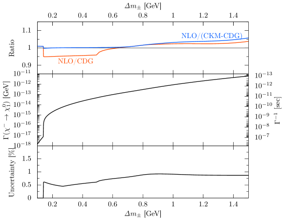
Figure 1: The NLO chargino decay rate into one of the neutralinos for a 300 GeV Higgsino, including the associated uncertainty, is presented in the middle and bottom panel. The red line in the top panel depicts the ratio of our NLO result to the previous CDG estimate. In contrast, the blue line indicates the ratio to the CDG estimate corrected for the inclusion of the CKM matrix and the single Kaon mode. The data are available at https://member.ipmu.jp/satoshi.shirai/Chargino_Decay/.

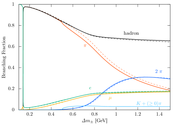
Figure 2: The branching fractions of each decay mode for 300 GeV Higgsino/Wino together with comparison with previous estimate by CDG. Our NLO results are shown by the solid lines and CDG’s results are represented by the dashed lines. The black solid line shows the sum of all the hadronic modes. The black dashed line represents the sum of the $2\pi$ and $3\pi$ modes estimated by CDG. The Kaon modes, which are not included in the CDG analysis, have a few percent branching fraction.

Before discussing details of our analysis, we first summarize the key findings of this paper. Fig. 1 displays the NLO chargino decay rate into one of the neutralinos for a 300 GeV Higgsino, including the associated uncertainties. Additionally, we provide a comparison with the previous estimates made by Chen, Drees, and Gunion (abbreviated as CDG) [24]. The NLO decay rates for other parameter points are available from the URL in Fig. 1.

When the charged Higgsino is capable of decaying into another neutral Higgsino, it is essential to include this decay rate to calculate the chargino lifetime. In the scenario of a pure Higgsino, for instance, the rate should be doubled. Furthermore, we have ascertained that the NLO correction to the decay rate is identical for both the Higgsino and the Wino. As a result, the decay rate depicted in the figure can be adapted for the charged Wino case by multiplying it by four.

As we will explain in subsection 4.3, the “tree-level” or leading-order (LO) approximation to the decay rates suffers from more than about 7% uncertainty. The NLO computation reduces this uncertainty substantially. The remaining uncertainties come from theoretical estimation of the long-distance corrections and the experimental errors of the hadronic spectral functions. As a result, we provide the decay width at a precision less than 1% for a wide range of mass difference.

The original CDG analysis does not account for the effect of the CKM matrix element. This omission leads to an approximate 5% deviation in the decay rate compared to our results, as illustrated by the red line in Fig. 1. We also present the CDG decay rate, now corrected by incorporating the CKM matrix. Additionally, we have extended their analysis on the pion mode to include the single Kaon mode, as represented by the blue line in Fig. 1. After these corrections, our results are about 3% larger than the CDG estimate for the mass difference larger than 1 GeV. These differences come from the multi-meson modes.

Fig. 2 illustrates the branching fractions of each decay mode, along with a comparison to the previous estimates by CDG. Our updated results are depicted using solid lines, while CDG’s results are represented by dashed lines. Our new estimate slightly deviates from CDG results for the hadronic modes. The deviation mainly comes from the difference of the hadronic spectral functions. The Kaon modes, which were not included in the CDG analysis, also affect the branching fractions.

Application to Wino Decay Rate

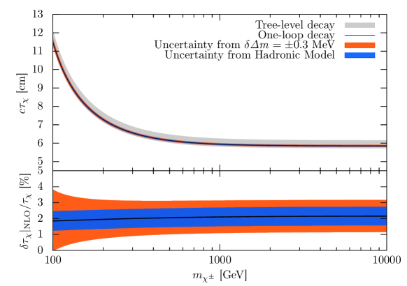
Figure 3: The decay length of the Wino as a function of its mass, denoted as $m_{\chi^{\pm}}$, is depicted using black solid lines. These lines represent the NLO estimation with the mass difference approximated at the two-loop level, approximately given by $\mathit{\Delta}m_{\pm}\simeq 160\,\mathrm{MeV}$. The blue bands illustrate the uncertainty of our one-loop estimation due to strong dynamics. In contrast, the gray band indicates the error in the tree-level analysis, which has been significantly reduced in the NLO analysis. Additionally, the red bands represent the uncertainty arising from the three-loop correction to the Wino mass difference, quantified as $\delta\mathit{\Delta}m=\pm 0.3\,\mathrm{MeV}$, as discussed in Ref. [22]. Here, we define $\delta\tau_{\chi}|_{\mathrm{NLO}}:=\tau_{\chi}|_{\mathrm{NLO}}-\tau_{\chi}|_{\mathrm{LO}}$.

The present NLO calculation can be applied to the Wino, yielding a result that suggests the Higgsino rate should be multiplied by four. In Fig. 3, we show the result of the NLO Wino decay length. The black line shows the NLO prediction of the Wino decay length for a given chargino mass. The blue bands around the black solid line show the uncertainty of the NLO decay rate estimation from the strong dynamics. The gray band shows the uncertainty of the case of the LO calculation which is reduced to the blue band by the NLO analysis.

In the figure, we have used the prediction on $\mathit{\Delta}m_{\pm}$ at the two-loop for the pure Wino in Ref. [22] (see also Ref. [25]), adopting a fitting formula

$$\mathit{\Delta}m_{\pm}/\mathrm{MeV}|_{\mathrm{tree}}=\frac{21.8641+8.68343t+0.0568066t^{2}}{1+0.0530366t+0.000345101t^{2}}~{}~{}~{}\left(t=\frac{m_{\chi^{\pm}}}{\mathrm{GeV}}\right)\ .$$ (2.1)

This fitting formula provides a stable fitting for $m_{\chi}>90$ GeV. In the figure, the red band shows the uncertainty of the lifetime from the higher loop corrections to the Wino mass difference, $\delta\mathit{\Delta}m_{\pm}$ = 0.3 MeV, in Ref. [22].

Our calculation can be used for more general mass splitting for the Wino. However, for the Wino, achieving a substantial mass difference between the neutralino and chargino, larger than the size of the radiative correction, proves challenging. The mass splitting of the Wino is heavily suppressed by the Higgsino mass,

$$\mathit{\Delta}m_{\pm}=\frac{m_{Z}^{4}s_{2\beta}^{2}s_{W}^{2}c_{W}^{2}}{(M_{1}-M_{2})\mu^{2}}\simeq\frac{140\,\mathrm{MeV}}{\tan^{2}\beta}\quantity(\frac{300\,\mathrm{GeV}}{M_{1}-M_{2}})\quantity(\frac{1\,\mathrm{TeV}}{\mu})^{2}\ .$$ (2.2)

Definitions of the parameters in this equation are given in Sec. 3. A large mass difference necessitates a smaller Higgsino mass $\mu$, which in turn would make the Wino significantly deviate from the electroweak gauge interaction eigenstates. As a result, our NLO calculation is not applicable in such scenarios.

Update from Previous Study

Let us summarize the main points of the update from Ref. [23];

• The wave function renormalization factors in the heavy Wino limit used in the short distance correction are changed to those given in Appendix A.

• We include the uncertainty of $f_{VW}$ in the analysis of the single pion mode (see subsubsection 6.6.3).

• We include the NLO decay rate into the lepton mode.

• We include the Kaon mode as well as multi-hadron modes with short-distance NLO corrections.

3 Model of Higgsino Dark Matter

In this paper, we perform the NLO analysis of the chargino decay rate by taking the Higgsino as an example. As emphasised above, however, the following NLO results can be applied to the cases of the more general electroweak multiplets. To provide a detailed demonstration of the calculations, the Higgsino will serve as our illustrative case study. Discussions on applications to other generic electroweak-interacting particles will follow in subsequent sections.

Here, we summarize the set up of the Higgsino LSP scenario where the lightest neutralino and the chargino are dominated by the Higgsino (vector-like SU$(2)_{L}$ doublets fermion) contributions. Such a setup is realized when the gauginos and sfermions are rather heavy compared with the Higgsinos. In this limit, the mass splitting between the neutralinos as well as the mass difference between the neutralino-chargino are small, which is of $O(1)$ GeV or less for the gauginos and the sfermions in the multi-TeV range. In the following, we review the effective Lagrangian of the Higgsino sector obtained from the minimal SSM (MSSM) setup. The physical parameters used in our analysis are given in Table. 1.

Table 1: Physical parameters used in our analysis. We adopt the absolute values of the CKM matrix elements provided in Ref. [26]. The other parameters are taken from Ref. [27]. We use the weak mixing angle defined in the on-shell scheme in Eq. (4.1).

Quantity	Symbol	Value
QED fine-structure constant	$\alpha=e^{2}/(4\pi)$	1/137.035 999 084(21)
Fermi constant	$G_{F}$	$1.1663788\times 10^{-5}\,\mathrm{GeV}^{-2}$
$\absolutevalue{V_{ud}}$		0.974353(53)
$\absolutevalue{V_{us}}$		0.22500(23)
$W^{\pm}$-boson mass	$m_{W}$	80.379(12) GeV
$Z$-boson mass	$m_{Z}$	91.1876(21) GeV
$e$ mass	$m_{e}$	0.51099895000(15) MeV
$\mu$ mass	$m_{\mu}$	105.6583755(23) MeV
$\tau$ mass	$m_{\tau}$	1776.86(12) MeV
$\pi^{\pm}$ mass	$m_{\pi^{\pm}}$	139.57039(18) MeV
$\pi^{0}$ mass	$m_{\pi^{0}}$	134.9768(5) MeV
$K^{\pm}$ mass	$m_{K}$	493.677(13) MeV
Pion decay constant	$\sqrt{2}F_{\pi}\absolutevalue{V_{ud}}$	127.13(13) MeV
Kaon decay constant	$\sqrt{2}F_{K}\absolutevalue{V_{us}}$	35.09(5) MeV
Charged pion lifetime	$\tau_{\pi}$	$2.6033(5)\times 10^{-8}\,\mathrm{sec}$
Charged Kaon lifetime	$\tau_{K}$	$1.2380(20)\times 10^{-8}\,\mathrm{sec}$
$B(\pi^{\pm}\to\mu^{\pm}+\nu(+\gamma))$		$99.98770(4)$%
$B(K^{\pm}\to\mu^{\pm}+\nu(+\gamma))$		$63.56(11)$%

3.1 Mass Spectrum

In the MSSM, the Higgsinos $\tilde{H}_{u}$ and $\tilde{H}_{d}$ form the SU$(2)_{L}$ doublets,

$$\tilde{H}_{u}=\begin{pmatrix}\tilde{H}_{u}^{+}\\ \tilde{H}_{u}^{0}\end{pmatrix}\ ;\quad\tilde{H}_{d}=\begin{pmatrix}\tilde{H}_{d}^{0}\\ \tilde{H}_{d}^{-}\end{pmatrix}\ .$$ (3.1)

with hypercharges $1/2$ and $-1/2$, respectively. Here those fermions are the left-handed Weyl spinor. The mass term for the Higgsinos is given by

$$\mathcal{L}_{\mathrm{Higgsino\,\,mass}}=-\mu\epsilon^{ij}(\tilde{H}_{u})_{i}(\tilde{H}_{d})_{j}+\mathrm{h.c.}\ ,$$ (3.2)

where $\epsilon^{ij}$ is an antisymmetric tensor with $\epsilon^{12}=-\epsilon^{21}=+1$. The covariant derivative is given by

$$D_{\mu}=\partial_{\mu}-igt^{a}W^{a}_{\mu}-ig^{\prime}Q_{Y}B_{\mu}\ ,$$ (3.3)

where $g$ and $g^{\prime}$ denote the gauge coupling constants of SU(2)${}_{L}\times$U(1)_Y gauge interactions, $t^{a}$ the halves of the Pauli matrices, $W_{\mu}^{a}(a=1,2,3)$ the SU(2)_L gauge bosons, $Q_{Y}$ the hypercharge, and $B_{\mu}$ the U(1)_Y gauge boson.

In the MSSM, the gauge-eigenstates of the neutralino $\psi^{0}$ and the chargino $\psi^{\pm}$ are given by

$$\psi^{0} =\quantity(\tilde{B},\tilde{W}^{3},\tilde{H}_{d}^{0},\tilde{H}_{u}^{0})^{T};$$ (3.4)

$$\psi^{-} =\quantity(\tilde{W}^{-},\,\,\tilde{H}_{d}^{-})^{T};\,\,\,\psi^{+}=\quantity(\tilde{W}^{+},\,\,\tilde{H}_{u}^{+})^{T}\ ,$$ (3.5)

where $\tilde{W}^{3,\pm}$ and $\tilde{B}$ are the Winos and the Bino. Again, they are represented by two-component Weyl spinors. After the electroweak symmetry breaking, the mass terms of the neutralinos and the charginos are given by,

$$\mathcal{L}_{\text{neutralino mass}} =-\frac{1}{2}\quantity(\psi^{0})^{T}M_{\tilde{N}}\psi^{0}+\mathrm{h.c.}\ ;$$ (3.6)

$$\mathcal{L}_{\text{chargino mass}} =-\quantity(\psi^{-})^{T}M_{\tilde{C}}\psi^{+}+\mathrm{h.c.}\ .$$ (3.7)

Here $M_{\tilde{N}}$ is a $4\times 4$ complex symmetric matrix,

and $M_{\tilde{C}}$ is a $2\times 2$ complex matrix,

The complex parameters $M_{1,2}$ are the Bino and the Wino mass parameters and $\langle H_{u,d}^{0}\rangle$ are the vacuum expectation values of the neutral components of the up- and down-type Higgs bosons.

We can go to the diagonal basis of the neutralino by Takagi’s decomposition, that is, there exists a unitary matrix $N_{ia}$ such that

$$(M_{\tilde{N}})_{ab}=(N^{T})_{ai}\matrixquantity(m_{\tilde{N}_{1}}&&&\\ &m_{\tilde{N}_{2}}&&\\ &&m_{\tilde{N}_{3}}&\\ &&&m_{\tilde{N}_{4}})_{ij}N_{jb}\ ,$$ (3.8)

where the neutralino in the mass basis is given by

$$\tilde{N}_{i}=N_{ia}\psi^{0}_{a}\ .$$ (3.9)

Hereafter, $a,b=1,\cdots,4$ denote gauge interaction basis, and $i,j=1,\cdots,4$ denote the mass eigenbasis for the neutralinos. Similarly, we can find the mass basis of the charginos by the singular decomposition by a pair of unitary matrices $(U,V)$ such that

$$(M_{\tilde{C}})_{ab}=(U^{T})_{ai}\matrixquantity(m_{\tilde{C}_{1}}&\\ &m_{\tilde{C}_{2}})_{ij}V_{jb}\ .$$ (3.10)

The mass basis of the chargino can be defined by

$$\tilde{C}^{+}_{i}=V_{ia}\psi^{+}_{a}\ ,\quad\tilde{C}^{-}_{i}=U_{ia}\psi^{-}_{a}\ ,$$ (3.11)

with $a,b=1,2$ and $i,j=1,2$ being the gauge interaction and the mass eigenbasis, respectively. Here, $\tilde{N}_{3,4}$ and $\tilde{C}^{\pm}_{2}$ consist of the Higgsino-like states. When $M_{1,2}$ and $\mu$ are real-valued, the mass eigenvalues of them are given by

$$m_{\tilde{N}_{3}} =\mu-\frac{(1+s_{2\beta})m_{Z}^{2}}{2}\quantity(\frac{c_{W}^{2}}{M_{2}-\mu}+\frac{s_{W}^{2}}{M_{1}-\mu})+O({m_{Z}^{4}})\ ;$$ (3.12)

$$m_{\tilde{N}_{4}} =-\mu-\frac{(1-s_{2\beta})m_{Z}^{2}}{2}\quantity(\frac{c_{W}^{2}}{M_{2}+\mu}+\frac{s_{W}^{2}}{M_{1}+\mu})+O({m_{Z}^{4}})\ ;$$ (3.13)

$$m_{\tilde{C}_{2}} =\mu-\frac{c_{W}^{2}m_{Z}^{2}(s_{2\beta}M_{2}+\mu)}{M_{2}^{2}-\mu^{2}}+O({m_{Z}^{4}})\ .$$ (3.14)

Here, $s_{W}$ and $c_{W}$ stand for $\sin\theta_{W}$ and $\cos\theta_{W}$ with $\theta_{W}$ being the weak mixing angle, respectively. The $Z$-boson mass is denoted by $m_{Z}$. The ratio of the Higgsino mass is defined by $\tan\beta=\langle H_{u}^{0}\rangle/\langle H_{d}^{0}\rangle>0$ with $s_{2\beta}=\sin 2\beta$. Note that we take the mass eigenvalues $m_{\tilde{N}_{i},\tilde{C}_{i}}$ are complex valued in general and the mass ordering is not determined.

In the following, we consider a heavy gaugino scenario, specifically $|M_{1,2}|\gg|\mu|$, where the Higgsino-like neutralinos $\chi^{0}_{1,2}$ are ordered based on the tree-level mass parameters:

$$m_{\chi^{0}_{1}} :=\min\left(|m_{\tilde{N}_{3}}|,|m_{\tilde{N}_{4}}|\right)\ ;$$ (3.15)

$$m_{\chi^{0}_{2}} :=\max\left(|m_{\tilde{N}_{3}}|,|m_{\tilde{N}_{4}}|\right)\ ,$$ (3.16)

and the Higgsino-like chargino $\chi^{-}$ is composed of $\tilde{C}_{2}^{\pm}$ with a tree-level mass defined by

$$m_{\chi^{\pm}}:=\absolutevalue{m_{\tilde{C}_{2}}}\ .$$ (3.17)

When $M_{1,2}$ and $\mu$ are real-valued, the mass difference between $\chi_{1,2}^{0}$ is given by

$$\mathit{\Delta}m_{0}^{\mathrm{tree}}:=m_{\chi^{0}_{2}}-m_{\chi^{0}_{1}}\simeq m_{Z}^{2}\quantity|\frac{c_{W}^{2}}{M_{2}}+\frac{s_{W}^{2}}{M_{1}}|\ ,$$ (3.18)

for $|M_{1,2}|\gg|\mu|$. The mass differences between the lightest $\chi_{1,2}^{0}$ and $\chi^{\pm}$ are given by

$$\mathit{\Delta}m_{\pm,1}^{\text{tree}} =m_{\chi^{\pm}}-m_{\chi_{1}^{0}}\simeq\frac{\mathit{\Delta}m_{0}^{\text{tree}}}{2}-\frac{1}{2}s_{2\beta}\,m_{Z}^{2}\left(\frac{c_{W}^{2}}{M_{2}}-\frac{s_{W}^{2}}{M_{1}}\right)\ ,$$ (3.19)

$$\mathit{\Delta}m_{\pm,2}^{\text{tree}} =m_{\chi^{\pm}}-m_{\chi_{2}^{0}}\simeq-\frac{\mathit{\Delta}m_{0}^{\text{tree}}}{2}-\frac{1}{2}s_{2\beta}\,m_{Z}^{2}\left(\frac{c_{W}^{2}}{M_{2}}-\frac{s_{W}^{2}}{M_{1}}\right)\ .$$ (3.20)

Thus, for $|M_{1,2}|$ in the TeV range and $\tan\beta\gg 1$, the neutralinos and the chargino are quasi-degenerate with mass differences of $O({1})$ GeV or smaller.

The radiative corrections also induce the chargino-neutralino mass splitting. As we assume the heavy gaugino/sfermions, the mass splitting from the radiative corrections is dominated by the electroweak contributions, which result in

$$\mathit{\Delta}m_{\pm}^{\text{rad}} \simeq\frac{\alpha_{\overline{\mathrm{MS}}}(m_{Z})\absolutevalue{\mu}}{2\pi}\int^{1}_{0}{\rm d}t(1+t)\log\left[1+\frac{m_{Z}^{2}(1-t)}{\absolutevalue{\mu}^{2}t^{2}}\right]\ ,$$ (3.21)

where $\alpha_{\overline{\mathrm{MS}}}(m_{Z})^{-1}=127.93$ is the $\overline{\mathrm{MS}}$ fine structure constant in the SM evaluated at the $Z$-boson mass. In the limit of $|\mu|\to\infty$,

$$\mathit{\Delta}m^{\text{rad}}_{\pm}\simeq 353\,\text{MeV}\ .$$ (3.22)

Here, we have included the two-loop corrections to the mass splitting, which is about $-3$ MeV in Ref. [21]. Note that when considering a finite Higgsino mass, the radiative mass splitting shows a mild mass dependence. This effect can influence the mass splitting by $O(10\%)$ for a Higgsino whose mass is on the order of the weak scale [15].

As a result, the mass differences between the neutralinos and the chargino are given by,

$$\mathit{\Delta}m_{\pm,i} =\mathit{\Delta}m_{\pm,i}^{\text{tree}}+\mathit{\Delta}m_{\pm}^{\text{rad}}\ ,$$ (3.23)

for $i=1,2$, respectively. As we are interested in the Higgsino-like dark matter scenario, we assume the spectrum

$$m_{\chi^{0}_{1}}<m_{\chi^{\pm}}\ ,$$ (3.24)

where the ordering between $\chi^{\pm}$ and $\chi_{2}^{0}$ is not specified.

3.2 Gauge Interaction

The charged Higgsino decay mediated by the Higgs and the sfermions are highly suppressed, and hence, the decay process is dominated by the $W$-boson exchange. In the two-component fashion, the gauge interactions with the $W$-boson, $W_{\mu}^{+}=(W_{\mu}^{1}-iW_{\mu}^{2})/\sqrt{2}$, are written by

$$\mathcal{L}_{\mathrm{MSSM}}\supset gW^{+}_{\mu}\quantity[\tilde{W}^{3\dagger}\bar{\sigma}^{\mu}\tilde{W}^{-}-\tilde{W}^{+\dagger}\bar{\sigma}^{\mu}\tilde{W}^{3}+\frac{1}{\sqrt{2}}\quantity(\tilde{H}_{d}^{0\dagger}\bar{\sigma}^{\mu}\tilde{H}_{d}^{-}+\tilde{H}_{u}^{+\dagger}\bar{\sigma}^{\mu}\tilde{H}_{u}^{0})]+\mathrm{h.c.}$$ (3.25)

We define four-component spinors for the Wino and Higgsino as

$$\begin{split}\Psi_{\tilde{W}}^{-}&=\matrixquantity(\tilde{W}^{-}\\ \tilde{W}^{+\dagger});\,\,\,\Psi_{\tilde{H}}^{-}=\matrixquantity(\tilde{H}^{-}_{d}\\ -\tilde{H}_{u}^{+\dagger});\\ \Psi_{\tilde{W}}^{0}&=\matrixquantity(\tilde{W}^{3}\\ \tilde{W}^{3\dagger});\,\,\,\Psi_{\tilde{H}_{d}}^{0}=\matrixquantity(\tilde{H}_{d}^{0}\\ \tilde{H}_{d}^{0\dagger});\,\,\,\Psi_{\tilde{H}_{u}}^{0}=\matrixquantity(\tilde{H}_{u}^{0}\\ \tilde{H}_{u}^{0\dagger}).\end{split}$$ (3.26)

Note that $\Psi^{0}_{\tilde{W}},\Psi^{0}_{\tilde{H}_{d}}$ and $\Psi^{0}_{\tilde{H}_{u}}$ are Majorana fields. In terms of these four-component fields, the gauge interactions are rewritten as

$$\mathcal{L}_{\mathrm{MSSM}}\supset gW^{-}_{\mu}\quantity[\bar{\Psi}^{-}_{\tilde{W}}\gamma^{\mu}\Psi^{0}_{\tilde{W}}+\frac{1}{\sqrt{2}}\quantity(\bar{\Psi}^{-}_{\tilde{H}}\gamma^{\mu}P_{L}\Psi^{0}_{\tilde{H}_{d}}+\bar{\Psi}^{-}_{\tilde{H}}\gamma^{\mu}P_{R}\Psi^{0}_{\tilde{H}_{u}})]+\mathrm{h.c.}$$ (3.27)

To express the mixings (3.9) and (3.11) in the four-component spinors, we introduce

$$\quantity(\Psi_{\tilde{C}})_{i}=\matrixquantity(\tilde{C}_{i}^{-}\\ \tilde{C}_{i}^{+\dagger})\ ;\,\,\,\quantity(\Psi_{\tilde{N}})_{j}=\matrixquantity(\tilde{N}_{j}\\ \tilde{N}^{\dagger}_{j})\ ,$$ (3.28)

whose mass terms are given by

$$\mathcal{L}_{\mathrm{MSSM}}\supset-m_{\tilde{C}_{i}}\quantity(\bar{\Psi}_{\tilde{C}})_{i}\quantity(\Psi_{\tilde{C}})_{i}-\frac{1}{2}m_{\tilde{N}_{j}}\quantity(\bar{\Psi}_{\tilde{N}})_{j}\quantity(\Psi_{\tilde{N}})_{j}\ ,$$ (3.29)

with $i=1,2$ and $j=1,\cdots 4$. We can readily see that

$$\begin{split}\Psi^{-}_{\tilde{W}}&=U^{*}_{i1}P_{L}\quantity(\Psi_{\tilde{C}})_{i}+V_{i1}P_{R}\quantity(\Psi_{\tilde{C}})_{i}\ ;\\ \Psi^{-}_{\tilde{H}}&=U^{*}_{i2}P_{L}\quantity(\Psi_{\tilde{C}})_{i}-V_{i2}P_{R}\quantity(\Psi_{\tilde{C}})_{i}\ ;\\ \Psi^{0}_{\tilde{W}}&=N^{*}_{j2}P_{L}\quantity(\Psi_{\tilde{N}})_{j}+N_{j2}P_{R}\quantity(\Psi_{\tilde{N}})_{j}\ ;\\ \Psi^{0}_{\tilde{H}_{d}}&=N^{*}_{j3}P_{L}\quantity(\Psi_{\tilde{N}})_{j}+N_{j3}P_{R}\quantity(\Psi_{\tilde{N}})_{j}\ ;\\ \Psi^{0}_{\tilde{H}_{u}}&=N^{*}_{j4}P_{L}\quantity(\Psi_{\tilde{N}})_{j}+N_{j4}P_{R}\quantity(\Psi_{\tilde{N}})_{j}\ .\end{split}$$ (3.30)

Therefore, we obtain

$$\mathcal{L}_{\mathrm{MSSM}}\supset gW^{+}_{\mu}\quantity(\bar{\Psi}^{0}_{\tilde{N}})_{j}\gamma^{\mu}\quantity[(O^{W}_{L})_{ji}P_{L}+(O^{W}_{R})_{ji}P_{R}](\Psi^{-}_{\tilde{C}})_{i}\ ,$$ (3.31)

where

$$(O^{W}_{L})_{ji}=N_{j2}U^{*}_{i1}+\frac{1}{\sqrt{2}}N_{j3}U^{*}_{i2}\ ;\quad(O^{W}_{R})_{ji}=N^{*}_{j2}V_{i1}-\frac{1}{\sqrt{2}}N^{*}_{j4}V_{i2}\ .$$ (3.32)

In the limit of $\absolutevalue{M_{1,2}}\gg\absolutevalue{\mu}\gg m_{Z}$, these mixing matrices are approximated as

$$(O^{W}_{L})_{32} \simeq\frac{1}{2}-\frac{(c_{\beta}^{2}-s_{\beta}^{2})}{8}\frac{m_{Z}^{2}(M_{1}c_{W}^{2}+M_{2}s_{W}^{2})}{M_{1}M_{2}\mu}\ ;\,\,\,(O^{W}_{R})_{32}\simeq\frac{1}{2}+\frac{(c_{\beta}^{2}-s_{\beta}^{2})}{8}\frac{m_{Z}^{2}(M_{1}c_{W}^{2}+M_{2}s_{W}^{2})}{M_{1}M_{2}\mu}\ ;$$ (3.33)

$$(O^{W}_{L})_{42} \simeq\frac{1}{2}+\frac{(c_{\beta}^{2}-s_{\beta}^{2})}{8}\frac{m_{Z}^{2}(M_{1}c_{W}^{2}+M_{2}s_{W}^{2})}{M_{1}M_{2}\mu}\ ;\,\,\,(O^{W}_{R})_{42}\simeq-\frac{1}{2}+\frac{(c_{\beta}^{2}-s_{\beta}^{2})}{8}\frac{m_{Z}^{2}(M_{1}c_{W}^{2}+M_{2}s_{W}^{2})}{M_{1}M_{2}\mu}\ ,$$ (3.34)

where we have assumed that $M_{1,2}$ and $\mu$ are real. Moreover, we find

$$(O^{W}_{L})_{32} \simeq\frac{1}{2}\quantity(1+\frac{\mathit{\Delta}m_{0}^{\mathrm{tree}}}{4\mu})\ ;\quad(O^{W}_{R})_{32}\simeq\frac{1}{2}\quantity(1-\frac{\mathit{\Delta}m_{0}^{\mathrm{tree}}}{4\mu})\ ,$$ (3.35)

$$(O^{W}_{L})_{42} \simeq\frac{1}{2}\quantity(1-\frac{\mathit{\Delta}m_{0}^{\mathrm{tree}}}{4\mu})\ ;\quad(O^{W}_{R})_{42}\simeq-\frac{1}{2}\quantity(1+\frac{\mathit{\Delta}m_{0}^{\mathrm{tree}}}{4\mu})\ ,$$ (3.36)

which are related to $\mathit{\Delta}m_{\pm,1}^{\mathrm{tree}}$ via $\mathit{\Delta}m_{\pm,1}^{\mathrm{tree}}=\mathit{\Delta}m_{0}^{\mathrm{tree}}/2$ for $\tan\beta\gg 1$. In this paper, we consider the case of the quasi-degenerate Higgsino, where $\absolutevalue{\mu}\gtrsim 100$ GeV and $\mathit{\Delta}m_{\pm,1}^{\mathrm{tree}}\lesssim O(1)$ GeV. In such a scenario, the $W$-boson interaction of the Higgsino-like states are close to those of the pure-Higgsino case. A similar observation can be made for the $Z$-boson interactions. Therefore, the gauge interactions of the Higgsino-like states can be well approximated as those of the pure Higgsinos. We will address effects on the Higgsino decay rate coming from the small mixing later.

4 Four-Fermion Interaction and Radiative Corrections

The decay process of the chargino is described by the effective four-fermion operators. To estimate its decay rate precisely, we should compute radiative corrections to the decay processes. Those corrections are composed of the electroweak, QED and QCD corrections. The electroweak interactions give rise to the short-distance corrections, whose computational framework we will show in this section. The perturbative QCD effects of ${O}(\alpha^{0}\alpha_{s})$ are absent from the short-distance corrections. The long-distance QED and QCD effects are discussed in Sec. 5 and Sec. 6.

In our analysis, we adopt the on-shell scheme of the electroweak theory [28]. The weak mixing angle $\theta_{W}$ is defined by

$$c_{W}=\cos\theta_{W}=\frac{m_{W}}{m_{Z}}\ ;\quad s_{W}=\sin\theta_{W}=\sqrt{1-\frac{m_{W}^{2}}{m_{Z}^{2}}}$$ (4.1)

to all order of perturbation, where $m_{W}$ and $m_{Z}$ are the physical masses of the $W$- and $Z$-bosons, respectively.

4.1 Tree-Level Four-Fermion Interaction

The gauge interactions of the chargino and neutralino exhibit a complex structure attributed to mass mixing, as detailed in Sec. 3. Nevertheless, in the pure-Wino/Higgsino scenario, the chargino decay can be examined within a simplified model at tree-level as outlined below.

We would like to discuss the weak decay of the chargino $\chi^{-}$ into a neutralino $\chi^{0}$ with emission of the SM particles, $\chi^{-}\to\chi^{0}+\mathrm{SM}$. We define the Dirac fermion $\Psi_{\chi^{-}}$ for the chargino and the Majorana fermion $\Psi_{\chi^{0}}$ for the neutralino. Their mass terms are written in the form of

$$\mathcal{L}_{\mathrm{mass}}=-m_{\chi^{\pm}}\overline{\Psi}_{\chi^{-}}\Psi_{\chi^{-}}-\frac{1}{2}m_{\chi^{0}}\overline{\Psi}_{\chi^{0}}\Psi_{\chi^{0}}\ .$$ (4.2)

We have rearranged the complex phases of the chargino/neutralino fields so that the mass parameters $m_{\chi^{\pm}}$ and $m_{\chi^{0}}$ are real and positive. In the Higgsino DM scenario, we have the two independent neutralinos, $\chi_{1}^{0}$ and $\chi^{0}_{2}$. In this case, the chargino mass is given by Eq. (3.17), whilst the neutralino mass is either Eqs. (3.15) or (3.16).

The decay of the chargino proceeds through the exchange of the $W$-boson, as we consider the scenario where all sparticles, except for the chargino and the neutralinos, are decoupled. In this case, the decay process would be characterized mainly by the mass difference,

$$\mathit{\Delta}m_{\pm}=m_{\chi^{\pm}}-m_{\chi^{0}}\ .$$ (4.3)

For $\mathit{\Delta}m_{\pm}\lesssim O(1)$ GeV, the $W$-boson exchange can be well approximated by the current-current operator,

$$\mathcal{L}_{\mathrm{CC}} =-2\sqrt{2}G_{F}J^{-\mu}_{\chi}J^{+}_{\mathrm{SM}\mu}+\mathrm{h.c.}\ ,$$ (4.4)

where $G_{F}$ denotes the Fermi constant determined by the muon decay [27], $J^{\mu}_{\chi}$ is the weak current of the chargino and the neutralino, and $J_{\mathrm{SM}}^{\mu}$ is the weak current composed of the SM quarks and the SM leptons. The small correction from the $W$-boson propagator is suppressed by $\quantity(\mathit{\Delta}m_{\pm}/m_{W})^{2}$ and can be safely neglected in the following discussion. By recalling that the mass mixing effects appear in the weak interaction as in Eq. (3.31), the weak current of the chargino and neutralino can be written as

$$J^{-\mu}_{\chi}=\sqrt{2}\,\overline{\Psi}_{\chi^{0}}\gamma^{\mu}\quantity(O^{W}_{L}P_{L}+O^{W}_{R}P_{R})\Psi_{\chi^{-}}\ ,$$ (4.5)

where $O_{L,R}^{W}$ are complex constants. We can rotate away the complex phases of $O_{L,W}^{W}$ which are relevant for the chargino decay. We follow the convention on the phases so that 

$$\begin{split}&O_{L}^{W}=+1\ ;\quad O_{R}^{W}=+1\quad\text{(pure-Wino case)}\ ;\\ &O_{L}^{W}=+\frac{1}{2}\ ;\quad O_{R}^{W}=+\frac{1}{2}\quad\text{(pure-Higgsino case)}\ .\end{split}$$ (4.6)

The weak charged current of the $u,d,s$-quarks and the leptons $\ell,\nu_{\ell}$ is given by

$$J_{\mathrm{SM}}^{+\mu}=V^{*}_{ud}\overline{\Psi}_{d}\gamma^{\mu}P_{L}\Psi_{u}+V^{*}_{us}\overline{\Psi}_{s}\gamma^{\mu}P_{L}\Psi_{u}+\overline{\Psi}_{\ell}\gamma^{\mu}P_{L}\Psi_{\nu_{\ell}}\ ,$$ (4.7)

where $V_{uD}\,(D=d,s)$ is the CKM matrix element and the SM particles are denoted by four-component spinors.

Since we consider cases that $\mathit{\Delta}m_{\pm}\lesssim O(1)$ GeV, we have to treat the quarks in the final state as hadrons (See Fig. 4(b)-4(d) ).

(a)

(b)

(c)

(d)

Figure 4: Example diagrams of chargino decay

Then, the decay channels for the chargino-neutralino mass difference less than $O(1)$ GeV are

• Leptonic modes ($\chi^{-}\to\chi^{0}+e/\mu+\bar{\nu}$, Sec. 5)

• Single pion mode ($\chi^{-}\to\chi^{0}+\pi^{-}$, Sec. 6)

• Single Kaon and multi-meson modes ($\chi^{-}\to\chi^{0}+K^{-}$ and $\chi^{-}\to\chi^{0}+(\geq 2)P,\,(P=\pi,K)$, Sec. 7)

For a detailed discussion of each decay mode, see the sections indicated in the parentheses. In the following, we calculate the universal short-distance corrections, which is a common contribution for all the modes.

4.2 Electroweak Correction to Four-Fermion Interaction

We calculate the short-distance correction to the four-fermion interactions. We are interested in corrections of $\mathcal{O}\quantity(\alpha)$ and neglect the contributions suppressed by $\quantity(\mathit{\Delta}m_{\pm}/m_{W})^{2}$. In this approximation, we can adopt the pure-Higgsino/Wino theory to estimate the electroweak corrections.

In the following, we will provide a detailed description of the pure-Higgsino case. The pure-Higgsino theory is defined by the following Lagrangian,

$$\mathcal{L}_{\mathrm{tree}}^{\mathrm{pure}}=\, \overline{\Psi}_{0}i\gamma^{\mu}\partial_{\mu}\Psi_{0}-m_{\chi}\overline{\Psi}_{0}\Psi_{0}+\bar{\Psi}_{-}i\gamma^{\mu}\partial_{\mu}\Psi_{-}-m_{\chi}\overline{\Psi}_{-}\Psi_{-}$$

$$+\frac{e}{c_{W}s_{W}}\quantity(\frac{1}{2}\overline{\Psi}_{0}\gamma^{\mu}\Psi_{0}-\frac{1}{2}\overline{\Psi}_{-}\gamma^{\mu}\Psi_{-}+s_{W}^{2}\overline{\Psi}_{-}\gamma^{\mu}\Psi_{-})Z_{\mu}-e\overline{\Psi}_{-}\gamma^{\mu}\Psi_{-}A_{\mu}$$

$$+\frac{e}{\sqrt{2}s_{W}}\overline{\Psi}_{-}\gamma^{\mu}\Psi_{0}W^{-}_{\mu}+\frac{e}{\sqrt{2}s_{W}}\overline{\Psi}_{0}\gamma^{\mu}\Psi_{-}W^{+}_{\mu}\ .$$ (4.8)

Here, $m_{\chi}$ is the SU$(2)$-symmetric mass parameter, which is taken to be equal to the physical charged Higgsino mass $m_{\chi^{\pm}}$ by tuning the $\mathrm{SU}(2)$ symmetric mass counterterm. The charged and neutral pure-Higgsinos are represented by the Dirac fields, $\Psi_{-}$ and $\Psi_{0}$, respectively. These two fields form the SU(2)_L doublet with the U(1)_Y hypercharge $-1/2$. We choose the phases of $\Psi_{-}$ and $\Psi_{0}$ so that $m_{\chi}$ is real and positive. We can see the equivalence to the gauge interactions written in the basis described in subsection 3.2 by the replacement

$$m_{\chi}=\mu\ ;\quad\Psi_{-}=i\quantity(\Psi_{\tilde{C}})_{2}\ ;\quad\Psi_{0}=\frac{i}{\sqrt{2}}\quantity[\quantity(\Psi_{\tilde{N}}^{0})_{3}-\gamma_{5}\quantity(\Psi_{\tilde{N}}^{0})_{4}]\ .$$ (4.9)

The four-fermion operator relevant for the charged Higgsino decay is given by 

$$\mathcal{L}_{\mathrm{FF}}^{\mathrm{pure},0}=-2\sqrt{2}G_{F}^{0}\quantity(\overline{\Psi}_{0}\gamma^{\mu}\Psi_{-})\quantity(\overline{\Psi}_{f}\gamma_{\mu}P_{L}\Psi_{f^{\prime}})+\mathrm{h.c.}\ ,$$ (4.10)

where $f,f^{\prime}$ represent the SU$(2)_{L}$ SM doublet fermions and $G_{F}^{0}$ is defined by

$$G_{F}^{0} =\frac{e^{2}}{4\sqrt{2}s_{W}^{2}m_{W}^{2}}\ .$$ (4.11)

In the rest of this section, physical quantities with the superscript $0$ should be understood as those determined by $G_{F}^{0}$, not by the Fermi constant $G_{F}$. The $W$-boson mass $m_{W}$ is related to the Fermi constant as

$$G_{F}^{0}=G_{F}\times(1-\mathit{\Delta}r)\ ,$$ (4.12)

where $\mathit{\Delta}r=0.0354055$. At one-loop level, $\mathit{\Delta}r$ is given by [31] 

$$\mathit{\Delta}r|_{\text{1-loop}} =\frac{\alpha}{4\pi}\quantity(\displaystyle{\frac{\hat{\Sigma}_{WW}^{\mathrm{1PI}}(0)}{m_{W}^{2}}}+\frac{6}{s_{W}^{2}}+\frac{7-4s_{W}^{2}}{s_{W}^{4}}\log c_{W})\ .$$ (4.13)

Note that $\mathit{\Delta}r|_{\text{1-loop}}$ dominates $\mathit{\Delta}r$ by including higher-order QCD effects in the self-energy of $W$-boson $\quantity(\alpha/(4\pi))\times\hat{\Sigma}_{WW}^{\mathrm{1PI}}(0)$ [32].

By following Ref. [33], we compute the electroweak radiative correction to the tree-level amplitude,

$$\mathcal{M}_{\mathrm{tree}}^{0}=-2\sqrt{2}G_{F}^{0}\bar{u}_{0}(p_{2})\gamma^{\mu}u_{-}(p_{1})\bar{u}_{f}(p_{3})\gamma_{\mu}P_{L}v_{f^{\prime}}(p_{4})\ ,$$ (4.14)

where the momentum assignment is determined as $\chi^{-}(p_{1})\to\chi^{0}(p_{2})f(p_{3})\overline{f^{\prime}}(p_{4})$. To derive the matching conditions to the low-energy effective theories, we keep the QED charge difference $\overline{Q}=Q_{f}-\quantity(-Q_{f^{\prime}})$ arbitrary [34]. For the short-distance correction, the SM fermion masses in the final state can be safely neglected. In the following, therefore, we approximate the momenta as $p_{1}\simeq p_{2}$ and $p_{3,4}\simeq 0$.

The radiative corrections in electroweak theory are composed of wave-function renormalizations, box contributions, vertex corrections, and the self-energy of the virtual $W$-boson. We describe computational detail in Appendix A. In our analysis, we calculate the radiative corrections with the help of $\mathtt{FeynArts}$ [35], $\mathtt{FeynCalc}$ [36, *Shtabovenko:2016sxi, *Shtabovenko:2020gxv] and $\mathtt{Package\mbox{--}X}$ [39] through $\mathtt{FeynHelper}$ [40]. Putting all the contributions together, we can write down the electroweak corrections in the form of

$$\mathcal{M}_{\mathrm{Virtual(EW)}}^{0} =\mathcal{M}_{\mathrm{tree}}^{0}\times\frac{\alpha}{4\pi}\quantity[3\log\frac{m_{W}}{m_{\gamma}}+\frac{\hat{\Sigma}_{WW}^{\mathrm{1PI}}(0)}{m_{W}^{2}}+F^{\mathrm{Virtual(EW)}}_{V}(r_{W})]$$

$$\hskip 20.0pt+\mathcal{M}_{A}^{0}\times\frac{\alpha}{4\pi}F^{\mathrm{Virtual(EW)}}_{A}(r_{W})\ ,$$ (4.15)

where $r_{W}=m_{W}/m_{\chi^{\pm}}$, $\mathcal{M}_{A}^{0}$ is the axial current contribution given by

$$\mathcal{M}_{A}^{0}=-2\sqrt{2}G_{F}^{0}\bar{u}_{0}(p_{2})\gamma^{\mu}\gamma_{5}u_{-}(p_{1})\bar{u}_{f}(p_{3})\gamma_{\mu}P_{L}v_{f^{\prime}}(p_{4})\ ,$$ (4.16)

and $F_{V,A}^{\mathrm{Virtual(EW)}}(r_{W})$ represent non-logarithmic electroweak corrections.

For later use, we provide the analytical expression of $F_{V}^{\mathrm{Virtual(EW)}}(r_{W})$ here:

$$F_{V}^{\mathrm{Virtual(EW)}}(r_{W})=\frac{3(2-r_{W}^{2})}{2s_{W}^{2}}+\frac{2-s_{W}^{2}}{2s_{W}^{2}c_{W}^{2}}\times r_{W}^{4}\log r_{W}$$ (4.17)

$$\hskip 20.0pt+\frac{2(4-5s_{W}^{2}-2s_{W}^{4}+3s_{W}^{6})+(c_{W}^{2}-s_{W}^{2})r_{W}^{4}}{2s_{W}^{4}c_{W}^{2}}\log c_{W}$$ (4.19)

$$\hskip 20.0pt+\frac{8-4s_{W}^{2}+(1+s_{W}^{2})r_{W}^{2}(2-r_{W}^{2})}{2s_{W}^{4}}\times\frac{r_{W}}{\sqrt{4-r_{W}^{2}}}\cot^{-1}\quantity(\frac{r_{W}}{\sqrt{4-r_{W}^{2}}})$$ (4.20)

$$\hskip 20.0pt+\frac{-4(2-s_{W}^{2})c_{W}^{4}-2(1-3s_{W}^{2}+2s_{W}^{4})r_{W}^{2}+(c_{W}^{2}-s_{W}^{2})r_{W}^{4}}{2s_{W}^{4}c_{W}^{2}}$$ (4.21)

$$\hskip 40.0pt\times\frac{r_{W}}{\sqrt{4c_{W}^{2}-r_{W}^{2}}}\cot^{-1}\quantity(\frac{r_{W}}{\sqrt{4c_{W}^{2}-r_{W}^{2}}})\ .$$ (4.22)

Note that, in the degenerate limit $\mathit{\Delta}m_{\pm}\to 0$, the finite part of the one-loop electroweak corrections to the four-fermion interaction (4.10) is independent of the $\mathrm{SU}(2)_{L}\times\mathrm{U}(1)_{Y}$ representation of the chargino/neutralino multiplet (see Appendices A.1 and A.2).

Consequently, the short-distance correction factor described in Eq. (4.17) is universal to weak decays of colorless fermions with $|\mathit{\Delta}Q_{\mathrm{QED}}|=1$ and with small mass splitting. Therefore, our current results can be utilized for the Wino and quintuplet minimal dark matter [11, *Cirelli:2007xd, *Cirelli:2009uv] as well as for more generic electroweak-interacting dark matter [41], particularly in scenarios involving the mass degenerate limit.

The self-energy of the $W$-boson is removed by using the relation (4.12). In other words, the perturbative expansion can be rearranged as

$$\mathcal{M}_{\mathrm{1-loop}} =\mathcal{M}_{\mathrm{tree}}^{0}+\mathcal{M}_{\mathrm{Virtual(EW)}}^{0}$$

$$=\mathcal{M}_{\mathrm{tree}}+\quantity(\mathcal{M}_{\mathrm{tree}}^{0}-\mathcal{M}_{\mathrm{tree}}+\mathcal{M}_{\mathrm{Virtual(EW)}}^{0})\ ,$$ (4.23)

where $\mathcal{M}_{\mathrm{tree}}$ denotes the tree-level amplitude obtained by replacing $G_{F}^{0}$ with $G_{F}$ in Eq. (4.14). In this case, the electroweak correction is given by

$$\mathcal{M}_{\mathrm{Virtual(EW)}}:=\,\, \mathcal{M}_{\mathrm{tree}}^{0}-\mathcal{M}_{\mathrm{tree}}+\mathcal{M}_{\mathrm{Virtual(EW)}}^{0}$$ (4.24)

$$=\,\, \mathcal{M}_{\mathrm{tree}}\times\frac{\alpha}{4\pi}\quantity[3\log\frac{m_{W}}{m_{\gamma}}+F^{\mathrm{Virtual(EW)}}_{V}(r_{W})-\quantity(\frac{6}{s_{W}^{2}}+\frac{7-4s_{W}^{2}}{s_{W}^{4}}\log c_{W})]$$ (4.25)

$$+\mathcal{M}_{A}\times\frac{\alpha}{4\pi}F^{\mathrm{Virtual(EW)}}_{A}(r_{W})\ ,$$ (4.26)

where $\mathcal{M}_{A}$ also represents the amplitude (4.16) with $G_{F}^{0}$ replaced by $G_{F}$.

Finally, we would like to stress that these contributions become constant in the heavy chargino limit $m_{\chi^{\pm}}\to\infty$ in the radiative correction (4.25). This is physically sensible behaviour since the recoil energy received by the heavy neutralino in the final state is very small and the total decay rate should be insensitive to the chargino mass in the limit of $m_{\chi^{\pm}}\to\infty$. The situation is similar to the limiting behaviour argued by Appelquist-Carrazone’s decoupling theorem [42], but different from the theorem in that in our case the heavy particles are external ones. In our analysis, we assume the decoupling of external particles to all order, which will be used as a sanity check to our computation.

4.3 Ambiguities in Definition of “Tree-Level”

Figure 5: The NLO electroweak and short-distance QED correction factor $S_{\mathrm{EW}}^{\chi}$. This factor is universal to weak decays of colorless fermions with $|\mathit{\Delta}Q_{\mathrm{QED}}|=1$ and with small mass splitting. Therefore, $S_{\mathrm{EW}}^{\chi}$ is common to both the Wino and the Higgsino. The orange band shows the dependence of $S_{\mathrm{EW}}^{\chi}$ on the infrared cut-off $\mu_{\mathrm{IR}}$. The solid line represents the case of $\mu_{\mathrm{IR}}=m_{\rho}$.

As stressed in Introduction, there is an ambiguity in definition of the “tree-level” decay rate. Namely, we can adopt the four-fermion operator (4.4) using the Fermi constant $G_{F}$ instead of the operator (4.10) using $G_{F}^{0}$ defined by Eq. (4.11). The difference in the choice of the tree-level coupling introduces about 7% error in the decay rate:

$$\frac{G_{F}^{2}}{\quantity(G_{F}^{0})^{2}}-1\simeq 0.07\ .$$ (4.27)

We cannot determine which coupling to be used and hence the tree-level estimation has the uncertainty provided by Eq. (4.27) as long as we stick to the leading-order computation.

As we stated below Eq. (4.13), the difference between $G_{F}^{0}$ and $G_{F}$ is dominated by $\left.\mathit{\Delta}r\right|_{\mathrm{1-loop}}$ with higher-order QCD effects included in the $W$-boson self energy $\quantity(\alpha/(4\pi))\times\hat{\Sigma}_{WW}^{\mathrm{1PI}}(0)$. Hence, by using the NLO amplitude, Eq. (4.2) or Eq. (4.25), the result is almost free from the ambiguity (4.27).

We should also note that the constant $G_{F}^{0}$ can be defined in terms of the running weak gauge coupling constant renormalized at high energy scale. For example, the weak gauge coupling at the scale larger than 1 TeV results in the deviation of the “tree-level” decay rate by more than $5$%. Our NLO analysis resolves this uncertainty too since we obtained the renormalization scale independent virtual correction at the one-loop level (see Eq. (4.25)).

A caveat is that in Eqs. (4.2) and (4.25), the IR cutoff $m_{\gamma}$ still remains since so far we only computed the virtual corrections. These dependencies on the photon mass vanish if we include real emission processes. In this paper, we present the complete calculation of long-distance corrections for the leptonic mode and single pion mode in Sec. 5 and Sec. 6, respectively.

For later convenience, we introduce the multiplicative factor $S_{\mathrm{EW}}^{\chi}$ defined by,

$$S^{\chi}_{\mathrm{EW}}(\mu_{\mathrm{IR}})-1=\,\, \frac{\alpha}{4\pi}\quantity[6\log\frac{m_{W}}{\mu_{\mathrm{IR}}}+2F^{\mathrm{Virtual(EW)}}_{V}\quantity(\frac{m_{W}}{m_{\chi^{\pm}}})-2\quantity(\frac{6}{s_{W}^{2}}+\frac{7-4s_{W}^{2}}{s_{W}^{4}}\log c_{W})]$$ (4.28)

$$+O(\alpha^{2},\alpha\alpha_{s})\ ,$$ (4.29)

to encapsulate the electroweak and short-distance QED corrections above $\mu_{\mathrm{IR}}$ to the decay rates computed in terms of the Fermi constant $G_{F}$ rather $G_{F}^{0}$. Here, the logarithmic factor in $S_{\mathrm{EW}}^{\chi}$ arises from the renormalization group (RG) effect  and $\mu_{\mathrm{IR}}$ is some infrared cutoff. In Fig. 5, we show the dependence of $S_{\mathrm{EW}}^{\chi}-1$ on the chargino mass. The dependence of $S_{\mathrm{EW}}^{\chi}-1$ on $\mu_{\mathrm{IR}}$ (from $0.5\,\mathrm{GeV}$ to $1\,\mathrm{GeV}$) is depicted as the orange band. In the limit of $m_{\chi^{\pm}}\to\infty$, we obtain a numerical estimation with $\mu_{\mathrm{IR}}$ around the $\rho$ meson mass, $m_{\rho}=0.77$ GeV,

$$S_{\mathrm{EW}}^{\chi}-1\simeq\frac{\alpha}{4\pi}\cdot 6\log\quantity(\frac{0.77\,\mathrm{GeV}}{\mu_{\mathrm{IR}}})+7.88\times{10}^{-3}\ .$$ (4.30)

For the single Kaon and multi-meson modes, we will approximate electroweak corrections by multiplying the decay rates by $S_{\mathrm{EW}}(m_{\rho})$ without performing full one-loop computation, since the branching fractions of these modes are small.

5 Decay into Leptons

The chargino can decay into leptons if kinematically allowed. In this section, we review the tree-level decay rates and perform analytical computation of one-loop corrections to the leptonic decay.

5.1 Tree-Level Decay Rate

The chargino decays into a neutralino $\chi^{0}_{1}$ (or $\chi^{0}_{2}$ if possible) and leptons through the operators,

$$\mathcal{L}^{\mathrm{lepton}}_{\mathrm{CC}}=-4G_{F}\,\overline{\Psi}_{\ell}\gamma^{\mu}P_{L}\Psi_{\nu_{\ell}}\times\overline{\Psi}_{\chi^{0}}\gamma^{\mu}\quantity(O^{W}_{L}P_{L}+O^{W}_{R}P_{R})\Psi_{\chi^{-}}+\mathrm{h.c.}\ ,$$ (5.1)

where $\Psi_{\nu_{\ell}}$ and $\Psi_{\ell}$ are four-component spinors to indicate the neutrino and charged lepton. At tree-level, we obtain the decay rate,

$$\Gamma_{\mathrm{tree}}(\chi^{-}\to\chi^{0}\ell^{-}\overline{\nu}_{\ell})=\frac{G_{F}^{2}}{\quantity(2\pi)^{3}}\int_{m_{\ell}^{2}}^{(\mathit{\Delta}m_{\pm})^{2}}ds\,\frac{s^{3}}{m_{\chi^{\pm}}^{3}}\lambda_{\chi^{\pm}\chi^{0}}^{1/2}(s)\times K^{\mathrm{lep}}(s)\ ,$$ (5.2)

where $m_{\ell}$ is the charged lepton mass, $\lambda_{AB}(s)$ is the kinematical function defined by

$$\lambda_{AB}(s) =\lambda(1,m_{A}^{2}/s,m_{B}^{2}/s)\ ;$$ (5.3)

$$\lambda(a,b,c) =a^{2}+b^{2}+c^{2}-2ab-2bc-2ca\ ,$$ (5.4)

and

$$K^{\mathrm{lep}}(s) =\quantity(1-\frac{m_{\ell}^{2}}{s})^{2}\quantity[\quantity(\absolutevalue{O^{W}_{L}}^{2}+\absolutevalue{O^{W}_{R}}^{2})K_{1}^{\mathrm{lep}}(s)+\quantity(O^{W}_{L}O^{W*}_{R}+O^{W}_{R}O^{W*}_{L})K_{2}^{\mathrm{lep}}(s)]\ ;$$ (5.5)

$$K_{1}^{\mathrm{lep}}(s) =\frac{1}{6}\quantity{\quantity(\frac{m_{\chi^{\pm}}^{2}+m_{\chi^{0}}^{2}}{s}-1)\quantity(1-\frac{m_{\ell}^{2}}{s})+\quantity[\quantity(\frac{m_{\chi^{\pm}}^{2}-m_{\chi^{0}}^{2}}{s})^{2}-1]\quantity(1+\frac{2m_{\ell}^{2}}{s})}\ ;$$ (5.6)

$$K_{2}^{\mathrm{lep}}(s) =-\frac{m_{\chi^{\pm}}m_{\chi^{0}}}{s}\ .$$ (5.7)

If we consider the Higgsino DM scenario, that is, if we take the limit of $\absolutevalue{M_{1,2}}\gg\absolutevalue{\mu}\,(\gtrsim m_{Z})$, then the decay rate is approximated as

$$\Gamma_{\mathrm{tree}}(\chi^{-}\to\chi^{0}\ell^{-}\overline{\nu}_{\ell})=\Gamma^{\chi\to\ell}_{\mathrm{tree},m_{\ell}=0}\times f\quantity(\frac{m_{\ell}}{\mathit{\Delta}m_{\pm}})\quantity(1-\frac{3\mathit{\Delta}m_{\pm}}{2m_{\chi^{\pm}}})\quantity[1+O\quantity(\quantity(\frac{\mathit{\Delta}m_{\pm}}{\mu})^{2})]\ ,$$ (5.8)

where $\Gamma_{\mathrm{tree},m_{\ell}=0}^{\chi\to\ell}=G_{F}^{2}\quantity(\mathit{\Delta}m_{\pm})^{5}/(30\pi^{3})$ and the function

$$f(x)=\frac{1}{2}\quantity[(2-9x^{2}-8x^{4})\sqrt{1-x^{2}}+15x^{4}\tanh^{-1}\quantity(\sqrt{1-x^{2}})]$$ (5.9)

reflects the nonzero lepton mass. The $O\quantity((\mathit{\Delta}m_{\pm}/\mu)^{2})$ contribution in Eq. (5.8), which is negligible in the present setup, comes from the mass mixing $O_{L/R}^{W}\simeq 1/2$ and expansion of the integrand (5.5). We can obtain the decay rate into leptons in the pure-Wino case, $O_{L/R}^{W}\simeq 1$, by multiplying Eq. (5.8) by four.

As stressed in subsection 4.3, there is an ambiguity in definition of the “tree-level” decay rate coming from the difference between $G_{F}$ and $G_{F}^{0}$, $G_{F}^{2}/(G_{F}^{0})^{2}-1\simeq 0.07$. Although this ambiguity has been mostly resolved by the short-distance NLO corrections computed in Sec. 4, the dependence on the photon mass $m_{\gamma}$ remains. In the following, we perform the NLO computation of the long-distance corrections and will obtain a result free from the photon mass dependence.

5.2 Computation of Radiative Corrections

We compute NLO corrections to the lepton mode according to the following strategy. First of all, we define the effective Lagrangian described by the four-fermion operators, whose counterterms are tuned so that the four-fermion theory reproduces the on-shell amplitude in the electroweak theory. Next, we compute virtual-photon corrections and real-photon emissions based on the four-fermion theory defined above and obtain a UV and IR-finite result.

For definiteness, we assume the chargino and neutralino are Higgsino-like in this section. We can obtain the NLO leptonic decay rate of the Wino just by multiplying the result of the Higgsino case by four, because the radiative corrections are common to both cases up to $O(\alpha\mathit{\Delta}m_{\pm}/m_{\chi^{\pm}})$ contributions.

5.2.1 Effective Fermi Theory

We define the effective four-fermion theory of the Higgsinos,

$$\mathcal{L}_{\mathrm{FF}}^{\mathrm{lepton}}=\, -2G_{F}\quantity(\overline{\Psi}_{\ell}\gamma^{\mu}P_{L}\Psi_{\chi^{-}})\quantity(\overline{\Psi}_{\chi^{0}}\gamma_{\mu}P_{L}\Psi_{\nu_{\ell}})+4G_{F}\quantity(\overline{\Psi}_{\ell}P_{R}\Psi_{\chi^{-}})\quantity(\overline{\Psi}_{\chi^{0}}P_{L}\Psi_{\nu_{\ell}})+\mathrm{h.c.}\ ,$$ (5.10)

which is obtained by applying Fierz reorderings to Eq. (5.1) with $O_{L}^{W}=O_{R}^{W}=1/2$. The operator basis (5.10) is convenient for calculation of radiative corrections since the neutral fermion line is not affected by virtual photon exchanges. We add counterterms to the above four-fermion interaction as 

$$\delta\mathcal{L}_{\mathrm{FF}}^{\mathrm{lepton}}=\, -2G_{F}\delta_{V}^{L}\quantity(\overline{\Psi}_{\ell}\gamma^{\mu}P_{L}\Psi_{\chi^{-}})\quantity(\overline{\Psi}_{\chi^{0}}\gamma_{\mu}P_{L}{\nu_{\ell}})+4G_{F}\delta_{Y}^{R}\quantity(\overline{\Psi}_{\ell}P_{R}\Psi_{\chi^{-}})\quantity(\overline{\Psi}_{\chi^{0}}P_{L}\Psi_{\nu_{\ell}})+\mathrm{h.c.}$$ (5.11)

The electroweak corrections computed in Sec. 4 will be incorporated via the finite parts of these counterterms. That is, $\delta_{V}^{L}$ and $\delta_{Y}^{R}$ are determined so that the effective theory (5.10) reproduces the amplitude in the electroweak theory (4.25) when we neglect the lepton mass.

Here is a minor note on matching with the electroweak theory in the pure-Higgsino case. In the pure-Higgsino scenario, we have the two neutralinos $\chi_{1}^{0}$ and $\chi_{2}^{0}$ with different masses. In principle, the coefficients of the counterterms $\delta$’s should be prepared for each neutralino. Under the situation where the mass mixing effects are sufficiently small, we may use the $\delta$’s common to both $\chi^{0}_{1}$ and $\chi^{0}_{2}$ because the electroweak and QED interaction do not distinguish the two neutralinos. In addition, the two Majorana field, $\Psi_{\chi^{0}_{1}}$ and $\Psi_{\chi^{0}_{2}}$, can be collected into the single Dirac field of the pure-neutral Higgsino, which is denoted by $\Psi_{0}$ in Sec. 4. Therefore, the two copies of the Fermi theory defined by Eqs. (5.10) and (5.11) are equivalent to the Fermi theory of the pure-Higgsinos described by Dirac spinors,

$$\mathcal{L} \supset\mathcal{L}_{\mathrm{FF,lepton}}^{\mathrm{Dirac}}+\delta\mathcal{L}_{\mathrm{FF,lepton}}^{\mathrm{Dirac}}+\mathrm{h.c.}\ ;$$ (5.12)

$$\mathcal{L}_{\mathrm{FF,lepton}}^{\mathrm{Dirac}} =-2\sqrt{2}G_{F}\quantity(\overline{\Psi}_{\ell}\gamma^{\mu}P_{L}\Psi_{-})\quantity(\bar{\Psi}_{0}\gamma_{\mu}P_{L}\Psi_{\nu_{\ell}})+4\sqrt{2}G_{F}\quantity(\overline{\Psi}_{\ell}P_{R}\Psi_{-})\quantity(\overline{\Psi}_{0}P_{L}\Psi_{\nu_{\ell}})\ ;$$ (5.13)

$$\delta\mathcal{L}_{\mathrm{FF,lepton}}^{\mathrm{Dirac}} =-2\sqrt{2}G_{F}\delta_{V}^{L}\quantity(\overline{\Psi}_{\ell}\gamma^{\mu}P_{L}\Psi_{-})\quantity(\overline{\Psi}_{0}\gamma_{\mu}P_{L}\Psi_{\nu_{\ell}})+4\sqrt{2}G_{F}\delta_{Y}^{R}\quantity(\overline{\Psi}_{\ell}P_{R}\Psi_{-})\quantity(\overline{\Psi}_{0}P_{L}\Psi_{\nu_{\ell}})\ ,$$ (5.14)

which can be directly compared with the theory defined by Eq. (4.2).

By explicit computation, we find that these counterterms should be chosen as

$$\delta_{V}^{L}= \frac{\alpha}{4\pi}\quantity(\frac{3}{2}\log\frac{m_{W}^{2}}{m_{\chi^{\pm}}^{2}}-\frac{11}{4})$$ (5.15)

$$+\frac{\alpha}{4\pi}\quantity[F^{\mathrm{Virtual(EW)}}_{V}\quantity(\frac{m_{W}}{m_{\chi^{\pm}}})-\quantity(\frac{6}{s_{W}^{2}}+\frac{7-4s_{W}^{2}}{s_{W}^{4}}\log c_{W})-\left.F^{\mathrm{Virtual(EW)}}_{A}\quantity(\frac{m_{W}}{m_{\chi^{\pm}}})\right|_{\overline{Q}=-1}]\ ;$$ (5.16)

$$\delta_{Y}^{R}=\,\, -\frac{\alpha}{4\pi}\quantity(3\log\frac{\Lambda_{\mathrm{FF}}^{2}}{m_{\chi^{\pm}}^{2}}+\frac{3}{2}\log\frac{m_{W}^{2}}{m_{\chi^{\pm}}^{2}}-\frac{1}{4})$$ (5.17)

$$+\frac{\alpha}{4\pi}\quantity[F^{\mathrm{Virtual(EW)}}_{V}\quantity(\frac{m_{W}}{m_{\chi^{\pm}}})-\quantity(\frac{6}{s_{W}^{2}}+\frac{7-4s_{W}^{2}}{s_{W}^{4}}\log c_{W})+\left.F^{\mathrm{Virtual(EW)}}_{A}\quantity(\frac{m_{W}}{m_{\chi^{\pm}}})\right|_{\overline{Q}=-1}]\ ,$$ (5.18)

to reproduce the electroweak theory (see Eq. (4.25)). Here, $\Lambda_{\mathrm{FF}}$ is the Pauli-Villars regulator mass introduced to regularize the photon loop.

5.2.2 Virtual Corrections

Figure 6: Feynman diagrams of 1PI virtual corrections and counterterm contribution to the leptonic mode.

We perform computation of the virtual photon corrections including the finite lepton mass. These corrections consist of wave-function renormalizations, 1PI corrections, and counterterm contributions (for the last two contributions, see Fig. 6). The resultant one-loop corrections can be broken up into the three pieces:

$$\delta\Gamma^{\chi\to\ell}_{\mathrm{virtual}}=\delta\Gamma^{\chi\to\ell}_{\mathrm{SD(EW)}}+\delta\Gamma^{\chi\to\ell}_{\mathrm{virtual,IR}}+\delta\Gamma^{\chi\to\ell}_{\mathrm{LD(QED)}}\ .$$ (5.19)

The first term represents the electroweak non-logarithmic corrections provided by the counterterms,

$$\delta\Gamma^{\chi\to\ell}_{\mathrm{SD(EW)}} =\Gamma^{\chi\to\ell}_{\mathrm{tree}}\times\frac{\alpha}{4\pi}\cdot 2\quantity[F^{\mathrm{Virtual(EW)}}_{V}\quantity(\frac{m_{W}}{m_{\chi^{\pm}}})-\quantity(\frac{6}{s_{W}^{2}}+\frac{7-4s_{W}^{2}}{s_{W}^{4}}\log c_{W})]\ .$$ (5.20)

Here, $\Gamma^{\chi\to\ell}_{\mathrm{tree}}$ is the tree-level rate  in the limit of $\mathit{\Delta}m_{\pm}\ll m_{\chi^{\pm}}$:

$$\Gamma^{\chi\to\ell}_{\mathrm{tree}}=\Gamma_{\mathrm{tree},m_{\ell}=0}^{\chi\to\ell}\times\int_{x}^{1}dw\,\rho_{\mathrm{tree}}(w)\ ,$$ (5.21)

where $w$ is the charged lepton energy normalized by $\mathit{\Delta}m_{\pm}$, $x=m_{\ell}/\mathit{\Delta}m_{\pm}$, and

$$\rho_{\mathrm{tree}}(w) =30w^{2}(1-w)^{2}\sqrt{1-\frac{x^{2}}{w^{2}}}\ .$$ (5.22)

The second term $\delta\Gamma^{\chi\to\ell}_{\mathrm{IR(virtual)}}$ is the infrared divergent part,

$$\delta\Gamma^{\chi\to\ell}_{\mathrm{virtual,IR}} =4\log\frac{m_{\ell}^{2}}{m_{\gamma}^{2}}\times\frac{\alpha}{4\pi}\Gamma_{\mathrm{tree},m_{\ell}=0}^{\chi\to\ell}\int_{x}^{1}dw\,\rho_{\mathrm{tree}}(w)\quantity[1-\frac{w}{\sqrt{w^{2}-x^{2}}}\cosh^{-1}\quantity(\frac{w}{x})]\ ,$$ (5.23)

which will be canceled with real photon corrections.

The third term $\delta\Gamma^{\chi\to\ell}_{\mathrm{LD(QED)}}$ represents the long-distance corrections from the virtual photon exchange. In the limit of $\mathit{\Delta}m_{\pm}\ll m_{\chi^{\pm}}$, it is given by

$$\delta\Gamma^{\chi\to\ell}_{\mathrm{LD(QED)}}=\Gamma^{\chi\to\ell}_{\mathrm{tree},m_{\ell}=0}\times\frac{\alpha}{4\pi}\int_{x}^{1}dw\,\rho_{\mathrm{LD(QED)}}(w)\ ,$$ (5.24)

where

$$\rho_{\mathrm{LD(QED)}}(w)=\, \quantity(-\frac{5}{2}+3\log\frac{m_{W}^{2}}{m_{\ell}^{2}})\rho_{\mathrm{tree}}(w)$$

$$+120w^{2}(1-w)^{2}\quantity[\cosh^{-1}\quantity(\frac{w}{x})-\quantity(\cosh^{-1}\quantity(\frac{w}{x}))^{2}-\mathrm{Li}_{2}\quantity(\frac{2\sqrt{w^{2}-x^{2}}}{w+\sqrt{w^{2}-x^{2}}})]$$

$$-120x^{2}(1-w)^{2}\cosh^{-1}\quantity(\frac{w}{x})\ .$$ (5.25)

Note that the axial contribution from the interference between the axial and the tree-level amplitudes in Eqs. (4.14) and (4.16) is suppressed by $\alpha\cdot m_{\ell}/m_{\chi^{\pm}}$.

We find no divergent terms in the limit of $m_{\chi^{\pm}}\to\infty$ as in the case of the electroweak correction. However, the decay spectrum $\rho_{\mathrm{LD(QED)}}(w)$ has logarithmic singularities with respect to the charged lepton mass,

$$\rho_{\mathrm{LD(QED)}}(w)\xrightarrow[m_{\ell}\ll\mathit{\Delta}m_{\pm}]{}\, -6\log x\times\rho_{\mathrm{tree}}(w)$$ (5.26)

$$-120\quantity[\log x+\quantity(\log x)^{2}]\times w^{2}(1-w)^{2}$$ (5.27)

$$+240\log x\times w^{2}(1-w)^{2}\log(w+\sqrt{w^{2}-x^{2}})$$ (5.28)

$$=:\rho_{\mathrm{LD(QED)}}^{\mathrm{singular}}(w)\ ,$$ (5.29)

which correspond to divergences arising when the charged lepton and photon become collinear. According to the Kinoshita-Lee-Nauenberg (KLN) theorem [43, 44], if we include real photon emissions, such singularities in decay spectra will disappear after integrating them over the phase space. We will see that the cancellation of the mass singularities will actually occur in the next subsubsection.

5.2.3 Real Photon Emission

Figure 7: Feynman diagrams of real photon emissions in the leptonic mode.

For completeness, we calculate the real photon emission processes shown in Fig. 7. The resultant decay rate is composed of the infrared divergent part and finite part,

$$\Gamma^{\chi\to\ell}_{\mathrm{emit}}=\Gamma^{\chi\to\ell}_{\mathrm{emit,IR}}+\Gamma^{\chi\to\ell}_{\mathrm{emit,finite}}\ .$$ (5.30)

The infrared divergent part is given by

$$\Gamma^{\chi\to\ell}_{\mathrm{emit,IR}}=-4\log\frac{m_{\ell}^{2}}{m_{\gamma}^{2}}\times\frac{\alpha}{4\pi}\Gamma_{\mathrm{tree},m_{\ell}=0}^{\chi\to\ell}\int_{x}^{1}dw\,\rho_{\mathrm{tree}}(w)\quantity[1-\frac{w}{\sqrt{w^{2}-x^{2}}}\cosh^{-1}\quantity(\frac{w}{x})]\ ,$$ (5.31)

which exactly cancels the IR divergence in the virtual correction (5.23). In the limit of $\mathit{\Delta}m_{\pm}\ll m_{\chi^{\pm}}$, the part free from IR divergences is given by

$$\Gamma^{\chi\to\ell}_{\mathrm{emit,finite}}=\Gamma^{\chi\to\ell}_{\mathrm{tree},m_{\ell}=0}\times\frac{\alpha}{4\pi}\int_{x}^{1}dw\,\rho_{\mathrm{emit}}(w)\ ,$$ (5.32)

where

$$\rho_{\mathrm{emit}}(w) =240w^{2}(1-w)^{2}\quantity[-\log x+\log(1-w)]\quantity[-\sqrt{1-\frac{x^{2}}{w^{2}}}+\cosh^{-1}\quantity(\frac{w}{x})]$$ (5.33)

$$+120w^{2}(1-w)^{2}\sqrt{1-\frac{x^{2}}{w^{2}}}\,(1-2\log 2)$$ (5.34)

$$+240(\log 2)w^{2}(1-w)^{2}\cosh^{-1}\quantity(\frac{w}{x})$$ (5.35)

$$+120w^{2}(1-w)^{2}\cosh^{-1}\quantity(\frac{w}{x})\quantity[1+\log x-\log(2w)]$$ (5.36)

$$+120w^{2}(1-w)^{2}\quantity[\mathrm{Li}_{2}\quantity(-\sqrt{1-\frac{x^{2}}{w^{2}}})-\mathrm{Li}_{2}\quantity(\sqrt{1-\frac{x^{2}}{w^{2}}})]$$ (5.37)

$$+60w^{2}(1-w)^{2}\quantity[\mathrm{Li}_{2}\quantity(\frac{w+\sqrt{w^{2}-x^{2}}}{2w})-\mathrm{Li}_{2}\quantity(\frac{w-\sqrt{w^{2}-x^{2}}}{2w})]$$ (5.38)

$$+360w^{2}(1-w)^{2}\quantity[\sqrt{1-\frac{x^{2}}{w^{2}}}-\cosh^{-1}\quantity(\frac{w}{x})]$$ (5.39)

$$+10(1-w)^{3}\quantity[-8\sqrt{w^{2}-x^{2}}+(1+7w)\cosh^{-1}\quantity(\frac{w}{x})]\ .$$ (5.40)

This estimation includes hard photon emissions. As in the case of the virtual corrections, the spectrum does not depend on the chargino/neutralino mass in the limit of $m_{\chi^{\pm}}\to\infty$.

The decay spectrum (5.33) exhibits the mass singularity in the limit of $m_{\ell}\ll\mathit{\Delta}m_{\pm}$:

$$\rho_{\mathrm{emit}}(w)\xrightarrow[m_{\ell}\ll\mathit{\Delta}m_{\pm}]{}\, 120\log x\times w^{2}(1-w)^{2}$$ (5.41)

$$\hskip 10.0pt\times\quantity[2\sqrt{1-\frac{x^{2}}{w^{2}}}-\log(w+\sqrt{w^{2}-x^{2}})-2\log(1-w)-1+\log\frac{w}{2}]$$ (5.42)

$$+120(\log x)^{2}w^{2}(1-w)^{2}$$ (5.43)

$$+360\log x\times w^{2}(1-w)^{2}-10\log x\times(1-w)^{3}(1+7w)$$ (5.44)

$$=:\rho_{\mathrm{emit}}^{\mathrm{singular}}(w)\ .$$ (5.45)

However, after combining the limiting behaviour of the virtual correction (5.26) and integration over the phase space, we find

$$\int_{x}^{1}dw\,\quantity[\rho_{\mathrm{LD(QED)}}^{\mathrm{singular}}(w)+\rho_{\mathrm{emit}}^{\mathrm{singular}}(w)]=-10x+O(x^{2})\ .$$ (5.46)

That is, the mass singularities completely vanish and the result is regular at $x=m_{\ell}/\mathit{\Delta}m_{\pm}=0$, as argued by the KLN theorem.

5.2.4 NLO Decay Rate

By combining the virtual and real photon corrections, we obtain the inclusive decay rate at one-loop level in the limit of $\mathit{\Delta}m_{\pm}\ll m_{\chi^{\pm}}$:

$$\Gamma_{\mathrm{NLO}}\quantity(\chi^{-}\to\chi^{0}\ell^{-}\overline{\nu}_{\ell}(\gamma))=\Gamma_{\mathrm{tree}}\quantity(\chi^{-}\to\chi^{0}\ell^{-}\overline{\nu}_{\ell})+\delta\Gamma^{\chi\to\ell}_{\mathrm{one\mathchar 45\relax loop}}\ ,$$ (5.47)

where

$$\delta\Gamma^{\chi\to\ell}_{\mathrm{one\mathchar 45\relax loop}}=\Gamma^{\chi\to\ell}_{\mathrm{tree},m_{\ell}=0}\times\frac{\alpha}{4\pi}\int_{x}^{1}dw\,\rho_{\mathrm{one\mathchar 45\relax loop}}(w)\ ,$$ (5.48)

and

$$\rho_{\mathrm{one\mathchar 45\relax loop}}(w)=\,\, 2\quantity[F^{\mathrm{Virtual(EW)}}_{V}\quantity(\frac{m_{W}}{m_{\chi^{\pm}}})-\quantity(\frac{6}{s_{W}^{2}}+\frac{7-4s_{W}^{2}}{s_{W}^{4}}\log c_{W})]\rho_{\mathrm{tree}}(w)$$ (5.49)

$$+\rho_{\mathrm{LD(QED)}}(w)+\rho_{\mathrm{emit}}(w)\ .$$ (5.50)

5.3 Numerical Results

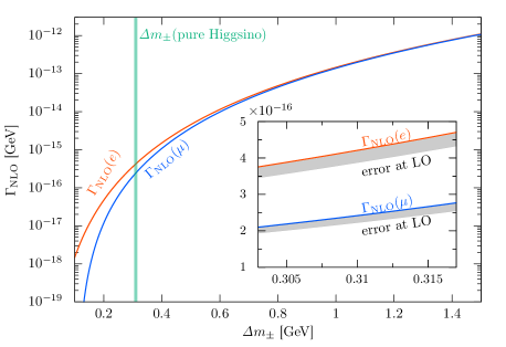
(a)

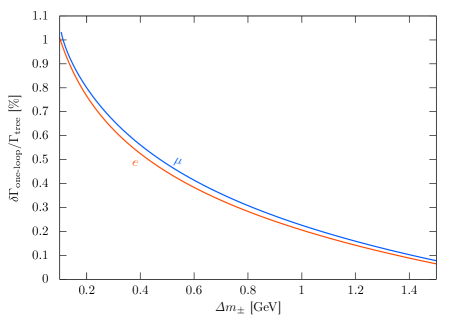
(b)

Figure 8: (Left) The NLO decay rate into the leptons as functions of $\mathit{\Delta}m_{\pm}$ in the case of $300$ GeV Higgsino. The blue and red line represent the muon and electron modes, respectively. The inserted window is the close-up view of the intersection between $\Gamma_{\mathrm{NLO}}$ and the vertical green band, which corresponds to the case of the 300 GeV pure-Higgsino. The gray bands represent the uncertainty of about 7% in the leading order decay rate (see Eq. (4.27)), which shrink to too small values to be shown in the NLO results. (Right) The ratio of the one-loop correction to the tree-level decay rate as functions of the mass difference for $m_{\chi^{\pm}}=300\,\mathrm{GeV}$.

In Fig. 8(a), we show the NLO decay rate of the 300 GeV Higgsino into the leptons as functions of $\mathit{\Delta}m_{\pm}$ for the muon mode (blue) and the electron mode (red). Here, only the decay to $\chi^{0}_{1}$ is considered; In the pure-Higgsino case, the decay rate should be multiplied by two. The decay rates in Fig. 8(a) are translated into the NLO decay rate of the charged Wino into the leptons just by multiplying the rate by four. The inserted window is the close-up view of the intersection between $\Gamma_{\mathrm{NLO}}$ and the vertical green band, which corresponds to the mass difference of the 300 GeV pure-Higgsino [45, 21, 15]. The gray bands represent the uncertainty of about 7% in the leading order decay rate (see Eq. (4.27)). The NLO calculation determines the decay rate to a precision of $O(\alpha/\pi\cdot\mathit{\Delta}m_{\pm}/m_{\chi^{\pm}})$.

In Fig. 8(b), we show the ratio of the one-loop correction to the tree-level decay rate as functions of the mass difference for the 300 GeV Higgsino. The NLO correction provides about $0.1$–$1$% modification to the tree-level rate.

6 Decay into Single Pion

In this section, we reanalyze the single pion mode of the chargino decay and update our previous estimate in Ref. [23] as mentioned in Sec. 2.

6.1 Tree-Level Decay Rate

The decay into the single charged pion $\pi^{\pm}$ is caused by the operators,

$$\mathcal{L}_{\mathrm{CC}}^{\mathrm{pion}}=-2\sqrt{2}\,G_{F}V_{ud}^{*}F_{\pi}(\partial_{\mu}\pi^{-})^{*}\times\overline{\Psi}_{\chi^{0}}\gamma^{\mu}\quantity(O^{W}_{L}P_{L}+O^{W}_{R}P_{R})\Psi_{\chi^{-}}+\mathrm{h.c.}\ ,$$ (6.1)

where $V_{ud}$ is the CKM matrix element and $F_{\pi}$ is the pion decay constant (see Table 1). When $\mathit{\Delta}m_{\pm}$ is larger than the charged pion mass $m_{\pi^{\pm}}$, the chargino $\chi^{-}$ can decay into a neutralino $\chi^{0}$ and a single pion $\pi^{-}$ through this coupling. The tree-level decay rate is given by

$$\Gamma_{\mathrm{tree}}\quantity(\chi^{-}\to\chi^{0}+\pi^{-})= \frac{F_{\pi}^{2}G_{F}^{2}\absolutevalue{V_{ud}}^{2}}{8\pi m_{\chi^{\pm}}}\sqrt{\lambda\quantity(1,m_{\chi^{0}}^{2}/m_{\chi^{\pm}}^{2},m_{\pi^{\pm}}^{2}/m_{\chi^{\pm}}^{2})}$$ (6.2)

$$\times\Bigg{\{}\absolutevalue{O^{W}_{L}+O^{W}_{R}}^{2}\quantity(m_{\chi^{\pm}}-m_{\chi^{0}})^{2}\quantity[\quantity(m_{\chi^{\pm}}+m_{\chi^{0}})^{2}-m_{\pi^{\pm}}^{2}]$$ (6.3)

$$\hskip 40.0pt+\absolutevalue{O^{W}_{L}-O^{W}_{R}}^{2}\quantity(m_{\chi^{\pm}}+m_{\chi^{0}})^{2}\quantity[\quantity(m_{\chi^{\pm}}-m_{\chi^{0}})^{2}-m_{\pi^{\pm}}^{2}]\Bigg{\}}\ ,$$ (6.4)

where $\lambda(a,b,c)$ is given by

$$\lambda(a,b,c)=a^{2}+b^{2}+c^{2}-2ab-2bc-2ca\ .$$ (6.5)

For the almost pure-Higgsino case that $\absolutevalue{M_{1,2}}\gg\absolutevalue{\mu}\gtrsim m_{Z}$, the above rate can be approximated as

$$\Gamma_{\mathrm{tree}}\quantity(\chi^{-}\to\chi^{0}+\pi^{-})=\, \frac{1}{\pi}F_{\pi}^{2}G_{F}^{2}\absolutevalue{V_{ud}}^{2}\quantity(\mathit{\Delta}m_{\pm})^{3}\sqrt{1-\quantity(\frac{m_{\pi^{\pm}}}{\mathit{\Delta}m_{\pm}})^{2}}$$ (6.6)

$$\times\quantity[1-\frac{\mathit{\Delta}m_{\pm}}{m_{\chi^{\pm}}}+\frac{\quantity(\mathit{\Delta}m_{\pm})^{2}-m_{\pi^{\pm}}^{2}}{4m_{\chi^{\pm}}^{2}}]^{3/2}\quantity[1+O\quantity(\quantity(\frac{\mathit{\Delta}m_{0}^{\mathrm{tree}}}{\mu})^{2})]\ ,$$ (6.7)

where $O\quantity((\mathit{\Delta}m_{0}^{\mathrm{tree}}/\mu)^{2})$ correction from the couplings $O_{L/R}^{W}$ stands for the deviation from the pure-Higgsino assumption.

6.2 “Tree-Level” and “Leading-Order” Decay Rates

As we have mentioned in Sec. 4.3, we face ambiguities in choice of the coupling constants of Lagrangian as long as we stick to the tree-level computation. Since the single pion mode is the most important decay mode for searches of the almost pure-Wino/Higgsino at collider experiments, we elucidate the ambiguities of the tree-level prediction of the decay rate to the single pion.

In subsection 6.1, we used the tree-level Lagrangian with the coefficient given by the Fermi constant $G_{F}$. We can also consider the tree-level decay rate with $G_{F}$ replaced by $G_{F}^{0}$ given by Eq. (4.11),

$$\Gamma^{0}_{\mathrm{tree}}\quantity(\chi^{-}\to\chi^{0}+\pi^{-}):=\left.\Gamma_{\mathrm{tree}}\quantity(\chi^{-}\to\chi^{0}+\pi^{-})\right|_{G_{F}\to G_{F}^{0}}\ .$$ (6.8)

Alternatively, we may consider the leading-order decay rate defined as the tree-level decay rate normalized by the $\pi_{\mu 2}$ decay rate, i.e., [22]

$$\Gamma_{\mathrm{LO}}\quantity(\chi^{-}\to\chi^{0}+\pi^{-}):=B\quantity(\pi^{-}\to\mu^{-}+\overline{\nu_{\mu}}(+\gamma))\times\Gamma^{\mathrm{tot}}_{\pi}\times\frac{\Gamma_{\mathrm{tree}}\quantity(\chi^{-}\to\chi^{0}+\pi^{-})}{\Gamma_{\mathrm{tree}}\quantity(\pi^{-}\to\mu^{-}+\overline{\nu_{\mu}})}\ ,$$ (6.9)

where

$$\Gamma_{\mathrm{tree}}\quantity(\pi^{-}\to\mu^{-}+\overline{\nu_{\mu}})=\frac{1}{4\pi}G_{F}^{2}\absolutevalue{V_{ud}}^{2}F_{\pi}^{2}m_{\pi^{\pm}}m_{\mu}^{2}\quantity(1-\frac{m_{\mu}^{2}}{m_{\pi^{\pm}}^{2}})^{2}\ ,$$ (6.10)

with $\Gamma^{\mathrm{tot}}_{\pi}=\tau_{\pi}^{-1}$ and $B(\pi^{-}\to\mu^{-}+\overline{\nu_{\mu}}(+\gamma))$ being the charged pion decay width and the branching fraction of the $\pi_{\mu 2}$ mode given in Table 1. Note that the dependence on $G_{F}\absolutevalue{V_{ud}}F_{\pi}$ is canceled in the ratio of the tree-level decay rates,

$$\frac{\Gamma_{\mathrm{tree}}\quantity(\chi^{-}\to\chi^{0}+\pi^{-})}{\Gamma_{\mathrm{tree}}\quantity(\pi^{-}\to\mu^{-}+\overline{\nu_{\mu}})}\simeq\, \frac{4\quantity(\mathit{\Delta}m_{\pm})^{3}}{m_{\pi^{\pm}}m_{\mu}^{2}}\sqrt{1-\quantity(\frac{m_{\pi^{\pm}}}{\mathit{\Delta}m_{\pm}})^{2}}\quantity[1-\frac{\mathit{\Delta}m_{\pm}}{m_{\chi^{\pm}}}+\frac{\quantity(\mathit{\Delta}m_{\pm})^{2}-m_{\pi^{\pm}}^{2}}{4m_{\chi^{\pm}}^{2}}]^{3/2}\quantity(1-\frac{m_{\mu}^{2}}{m_{\pi^{\pm}}^{2}})^{-2}\ .$$ (6.11)

When focusing on the “tree-level” decay rate, it is important to note that the three decay rates $\Gamma_{\mathrm{tree}}$, $\Gamma_{\mathrm{tree}}^{0}$, and $\Gamma_{\mathrm{LO}}$ are all considered “correct.” Numerically, however, we find that those tree-level decay rates differ by about 10%,

$$\frac{\Gamma_{\mathrm{tree}}\quantity(\chi^{-}\to\chi^{0}+\pi^{-})}{\Gamma_{\mathrm{LO}}\quantity(\chi^{-}\to\chi^{0}+\pi^{-})}\simeq 0.98\ ;\qquad\frac{\Gamma^{0}_{\mathrm{tree}}\quantity(\chi^{-}\to\chi^{0}+\pi^{-})}{\Gamma_{\mathrm{LO}}\quantity(\chi^{-}\to\chi^{0}+\pi^{-})}\simeq 0.91\ .$$ (6.12)

This uncertainty profoundly affects searches for meta-stable charginos at collider experiments, where the detection efficiency strongly depends on the chargino lifetime.

6.3 Prelude to Radiative Corrections: Two-step Matching Procedure

Figure 9: Flowchart of the matching procedure.

The decay into a single pion is described by the non-renormalizable interaction (6.1). In the presence of the QED interactions, the derivative in this operator should be replaced with the covariant one, $D_{\mu}=\partial_{\mu}-ieA_{\mu}$. As a result, we obtain the interaction term,

$$\mathcal{L}_{\mathrm{CC}}^{\mathrm{meson}}=-2\sqrt{2}\,G_{F}V_{ud}^{*}F_{\pi}\quantity(D_{\mu}\pi^{-})^{*}\times\overline{\Psi}_{\chi^{0}}\gamma^{\mu}\quantity(O_{L}^{W}P_{L}+O_{R}^{W}P_{R})\Psi_{\chi^{-}}+\mathrm{h.c.}$$ (6.13)

This theory can no longer be renormalized multiplicatively since the QED interaction explicitly violates the shift symmetry of the pion field.

We encounter a similar situation in the $\pi_{\ell 2}$ decay, which Knecht et al. [46] addressed within the framework of the chiral perturbation theory (ChPT). In that literature, the authors enumerate $O(e^{2}p^{2})$ low-energy constants (LECs) to the pion-lepton interactions. By using those LECs, they provide a UV-finite decay rate of the charged pion at one-loop level. Note that the finite part of the LECs cannot be determined unambiguously unless ChPT is matched with some UV-complete and renormalizable theory. Descotes-Genon and Moussallam [34] (hereafter referred to as D&M) match ChPT with the electroweak theory and fix the finite part of the LECs relevant for the $\pi_{\ell 2}$ decay.

In our previous analysis [23], we introduced the LECs $Y_{i}$ for the Wino-pion interaction following Ref. [46] and determined their finite parts by D&M’s matching procedure (See Fig. 9). First, we tune the counterterms of the intermediate four-fermion theory, $\mathcal{L}^{\mathrm{FF}}_{\mathrm{CT}}$, to reproduce the amplitude of the decay into the free quarks calculated by the electroweak theory including the Wino, $\mathcal{L}^{\mathrm{EW}}$. In the second step, we determine the LECs $Y_{i}$ in $\mathcal{L}_{\mathrm{CT}}^{\mathrm{ChPT+QED}}$ by matching ChPT with the four-fermion theory through the so-called current correlators. We found that the LECs $Y_{i}$ obtained by D&M’s matching method successfully provide the UV-finite Wino decay rate into a single pion.

As we will see in the following subsections, the computational framework used in the Wino case can be extended straightforwardly to more generic electroweak fermions including the Higgsino. In this case, we can safely neglect $O(\alpha\mathit{\Delta}m_{\pm}/m_{\chi^{\pm}})$ contributions in the computation of the radiative corrections. In addition, we can omit the mass mixing effect discussed in Sec. 3 because it is suppressed by $\alpha$ and the Wino or the Higgsino mass parameter. Therefore, the radiative corrections can be computed based on the pure-Higgsino/Wino Lagrangian. In the following analysis, we compute the radiative corrections to the decay rate of the charged Higgsino into a single pion based on the computational method used in Ref. [23].

6.4 Matching Four-Fermion Theory with Electroweak Theory

Following the analysis conducted by D&M, we introduce the intermediate step to define the four-fermion theory which reproduces the decay rate into free quarks under the electroweak interactions. The four-fermion theory obtained here will be matched with ChPT.

Let us consider the four-fermion theory with counterterms,

$$\mathcal{L} \supset\mathcal{L}_{\mathrm{FF,quark}}+\delta\mathcal{L}_{\mathrm{FF,quark}}+\mathrm{h.c.}\ ;$$ (6.14)

$$\mathcal{L}_{\mathrm{FF,quark}} =-2G_{F}V_{ud}^{*}(\overline{\Psi}_{d}\gamma^{\mu}P_{L}\Psi_{u})(\overline{\Psi}_{\chi^{0}}\gamma^{\mu}\Psi_{\chi^{-}})\ ;$$ (6.15)

$$\delta\mathcal{L}_{\mathrm{FF,quark}} =-2G_{F}V_{ud}^{*}(\overline{\Psi}_{d}\gamma^{\mu}P_{L}\Psi_{u})(\overline{\Psi}_{\chi^{0}}\gamma^{\mu}\Psi_{\chi^{-}})$$

$$\hskip 20.0pt\times e^{2}\quantity[f_{\chi\chi}Q_{\chi}^{2}+f_{d\bar{u}}(Q_{d}+Q_{\bar{u}})^{2}+f_{\chi d}Q_{\chi}Q_{d}-f_{\chi\bar{u}}Q_{\chi}Q_{\bar{u}}]\ ,$$ (6.16)

where $Q_{d}$ and $Q_{\bar{u}}$ are the charges of the $d$-quark and $u$-antiquark, respectively. The coefficients $f_{\chi\chi},f_{d\bar{u}},f_{\chi d}$, and $f_{\chi\bar{u}}$ should be determined by matching with the results of Sec. 4. It is important to leave the difference of the charges, $\overline{Q}=Q_{d}-Q_{\bar{u}}$, arbitrary to derive matching conditions.

As we noted in subsubsection 5.2.1, if we consider the case of the Higgsino-like DM, then we have the two Majorana neutralinos $\chi_{1}^{0}$ and $\chi_{2}^{0}$ with different masses and the counterterms should be prepared for each neutralino. However, since we address the situation where the mass mixings are sufficiently small, the two copies of the four-fermion theory (6.14) are equivalent to the four-fermion theory of the pure-Higgsinos,

$$\mathcal{L} \supset\mathcal{L}_{\mathrm{FF,quark}}^{\mathrm{Dirac}}+\delta\mathcal{L}_{\mathrm{FF,quark}}^{\mathrm{Dirac}}+\mathrm{h.c.}\ ;$$ (6.17)

$$\mathcal{L}_{\mathrm{FF,quark}}^{\mathrm{Dirac}} =-2\sqrt{2}G_{F}V_{ud}^{*}(\overline{\Psi}_{d}\gamma^{\mu}P_{L}\Psi_{u})(\overline{\Psi}_{0}\gamma^{\mu}\Psi_{-})\ ;$$ (6.18)

$$\delta\mathcal{L}_{\mathrm{FF,quark}}^{\mathrm{Dirac}} =-2\sqrt{2}G_{F}V_{ud}^{*}(\overline{\Psi}_{d}\gamma^{\mu}P_{L}\Psi_{u})(\overline{\Psi}_{0}\gamma^{\mu}\Psi_{-})$$

$$\hskip 20.0pt\times e^{2}\quantity[f_{\chi\chi}Q_{\chi}^{2}+f_{d\bar{u}}(Q_{d}+Q_{\bar{u}})^{2}+f_{\chi d}Q_{\chi}Q_{d}-f_{\chi\bar{u}}Q_{\chi}Q_{\bar{u}}]\ ,$$ (6.19)

where $\Psi_{-}$ and $\Psi_{0}$ are Dirac spinors for the charged and neutral Higgsinos, respectively. The four-fermion theory (6.17) can be directly compared with the theory defined by Eq. (4.2).

The decay amplitude of the chargino into free quarks can be computed at one-loop level based on the four-fermion theory (6.17). The QED correction generates the amplitude including the axial current of the chargino/neutralino, $\mathcal{M}_{A}^{\mathrm{quark}}$. As we pointed out in Ref. [23], however, the axial amplitude provides only two-loop-level contribution because the interference between $\mathcal{M}_{\mathrm{tree}}^{\mathrm{quark}}$ and $\mathcal{M}_{A}^{\mathrm{quark}}$ vanishes after integration over the phase space. Hence, we take into account only the one-loop level amplitude proportional to the tree-level one,

$$\frac{\mathcal{M}_{\mathrm{Virtual(FF)}}^{\mathrm{quark}}}{{\mathcal{M}}_{\mathrm{tree}}^{\mathrm{quark}}} =\frac{\alpha}{4\pi}\frac{3}{2}\quantity(\log\frac{\Lambda_{\mathrm{FF}}^{2}}{m_{\gamma}^{2}}-1)+e^{2}\left(f_{\chi\chi}+f_{d\bar{u}}+\frac{1-\overline{Q}}{2}f_{\chi d}-\frac{1+\overline{Q}}{2}f_{\chi\bar{u}}\right)\ ,$$ (6.20)

where $\Lambda_{\mathrm{FF}}$ is the Pauli-Villars regulator mass. We have set $Q_{\chi}=-1$ and $Q_{d}+Q_{\bar{u}}=-1$ while leaving $Q_{d}-Q_{\bar{u}}=\overline{Q}$ arbitrary. Since we use the bare fermion fields in this analysis, the virtual correction includes both the 1PI vertex corrections and the corrections to the two-point functions of the fermions. Note that unlike our previous analysis [23], we use the Pauli-Villars regularization to avoid the ambiguity in four-dimensional anti-symmetric tensor, $\epsilon_{\mu\nu\rho\sigma}$, in generic space-time dimension, which appears in the reduction of the UV divergent vertex correction.

By comparing the amplitude in the four-fermion theory (6.20) with the vector-like part of the amplitude in the electroweak theory (4.25), we get two independent matching conditions since the amplitude in the four-fermion theory (6.20) depends on the charge difference $\overline{Q}$: 

$$-e^{2}\frac{f_{\chi d}+f_{\chi\bar{u}}}{2} =0\ ;$$ (6.21)

$$e^{2}(f_{\chi\chi}+f_{d\bar{u}}+f_{\chi d}/2-f_{\chi\bar{u}}/2) =\frac{\alpha}{4\pi}\left[-\frac{3}{2}\quantity(\log\frac{\Lambda_{\mathrm{FF}}^{2}}{m_{W}^{2}}-1)\right.$$ (6.22)

$$\left.\hskip 20.0pt+F_{V}^{\mathrm{Virtual(EW)}}\quantity(\frac{m_{W}}{m_{\chi^{\pm}}})-\quantity(\frac{6}{s_{W}^{2}}+\frac{7-4s_{W}^{2}}{s_{W}^{4}}\log c_{W})\right]\ .$$ (6.23)

These counterterms incorporate the electroweak corrections into the four-fermion theory.

6.5 Matching ChPT with Four-Fermion Theory

We match the four-fermion theory obtained in the previous step with the extended ChPT including the charginos. We implement the procedure following D&M’s method. This step is essential as it yields integral representations of the LECs, which encapsulate vital information about the strong dynamics.

6.5.1 Contributions from Low-Energy Constants to Branching Fraction

The correction of the decay rate depends on three kinds of the LECs: $K_{i}$ for virtual photon introduced by Urech [47]; $X_{i}$ for virtual leptons enumerated by Knecht et al. [46]; $Y_{i}$ for virtual charginos obtained in parallel with $X_{i}$ [23]. The radiative correction of the chargino/pion’s decay rates depends on those LECs as

$$\left.\frac{\delta\Gamma_{\chi\to\pi}}{\Gamma_{\chi\to\pi}}\right|_{\mathrm{LEC}} =e^{2}\Bigg{[}\frac{8}{3}K_{1}+\frac{20}{9}K_{5}+4K_{12}$$ (6.24)

$$\hskip 85.35826pt-\hat{Y}_{6}-\frac{4}{3}(Y_{1}+\hat{Y}_{1})-4\left(Y_{2}+\hat{Y}_{2}-\frac{m_{{\chi^{\pm}}}}{\mathit{\Delta}m_{\pm}}Y_{3}\right)\Bigg{]}\ ;$$ (6.25)

$$\left.\frac{\delta\Gamma_{\pi}}{\Gamma_{\pi}}\right|_{\mathrm{LEC}} =e^{2}\Bigg{[}\frac{8}{3}K_{1}+\frac{20}{9}K_{5}+4K_{12}$$ (6.26)

$$\hskip 85.35826pt-\hat{X}_{6}-\frac{4}{3}(X_{1}+\hat{X}_{1})-4(X_{2}+\hat{X}_{2})+4X_{3}\Bigg{]}\ .$$ (6.27)

For the definitions of these LECs, consult subsection 5.1 of Ref. [23]. Here, we show LECs needed to cancel UV divergences arising from virtual photon exchange without taking the ratio between the chargino and pion decay rates. 

We would like to stress that we do not have to determine these LECs individually. In addition, as we can see from Eqs. (6.24) and (6.26), the radiative corrections to the branching ratio (6.11) does not depend on $K_{i}$ at all and are free from uncertainties from these LECs. In our analysis, therefore, the NLO decay rate is given in the form,

$$\Gamma_{\mathrm{NLO}}\quantity(\chi^{-}\to\chi^{0}+\pi^{-}(+\gamma))=\Gamma_{\mathrm{LO}}\quantity(\chi^{-}\to\chi^{0}+\pi^{-})\times\quantity(1+\frac{\delta\Gamma_{\chi\to\pi}}{\Gamma_{\chi\to\pi}}-\frac{\delta\Gamma_{\pi}}{\Gamma_{\pi}})\ ,$$ (6.28)

where

$$\Gamma_{\chi\to\pi}:=\Gamma_{\mathrm{tree}}\quantity(\chi^{-}\to\chi^{0}+\pi^{-})\ ;\quad\Gamma_{\pi}:=\Gamma_{\mathrm{tree}}\quantity(\pi^{-}\to\mu^{-}+\overline{\nu_{\mu}})\ ,$$ (6.29)

and $\delta\Gamma_{\chi\to\pi}$ and $\delta\Gamma_{\pi}$ stand for the radiative corrections to these tree-level decay rates.

6.5.2 Current Correlator with Minimal Resonance

To estimate numerically the above LECs’ contributions, we have to introduce a model to describe hadronization effects. From the discussion in the previous section, we find that the combinations of LECs relevant for our discussion are given by $X_{2}+\hat{X}_{2}-X_{3}$, $X_{1}+\hat{X}_{1}$, $Y_{2}+\hat{Y}_{2}-\quantity(m_{\chi^{\pm}}/\mathit{\Delta}m_{\pm})Y_{3}$, and $Y_{1}+\hat{Y}_{1}$. By using D&M’s method, we find that $X_{2}+\hat{X}_{2}-X_{3}$ and $X_{1}+\hat{X}_{1}$ are related to the current correlation functions in the momentum space,

$$if^{abc}\Gamma_{VA}^{\mu\nu}(\ell,r):=\int d^{4}xe^{i\ell x}\langle 0|TJ_{V}^{b\mu}(x)J_{A}^{c\nu}(0)|\pi^{a}(r)\rangle$$ (6.30)

and

$$d^{abc}\Gamma_{VV}^{\mu\nu}(\ell,r) :=\int d^{4}xe^{i\ell x}\langle 0|TJ_{V}^{b\mu}(x)J_{V}^{c\nu}(0)|\pi^{a}(r)\rangle\ ,$$ (6.31)

respectively. Here, $r$ is the pion momentum. The vector- and the axial-vector currents of the light quarks $\Psi_{q}=\quantity(\Psi_{u},\Psi_{d},\Psi_{s})^{T}$ are given by

$$J_{V}^{a\mu}=\overline{\Psi}_{q}\gamma^{\mu}t^{a}\Psi_{q}\ ;\quad J_{A}^{a\mu}=\overline{\Psi}_{q}\gamma^{\mu}\gamma^{5}t^{a}\Psi_{q}\ ,$$ (6.32)

where $t^{a}=\lambda^{a}/2$ with $\lambda^{a}$ being the Gell-Mann matrix, and $f^{abc}$ and $d^{abc}$ are the structure constants given by,

$$f^{abc}=-2i\mathop{\rm tr}[t^{a},[t^{b},t^{c}]]\ ,\quad d^{abc}=2\mathop{\rm tr}[t^{a},\{t^{b},t^{c}\}]\ .$$ (6.33)

Similarly, the combinations relevant for the chargino decay, $Y_{2}+\hat{Y}_{2}-\quantity(m_{\chi^{\pm}}/\mathit{\Delta}m_{\pm})Y_{3}$ and $Y_{1}+\hat{Y}_{1}$, can be connected to the current correlation functions

$$if^{abc}\overline{\Gamma}_{VA}^{\mu\nu}(\ell,r):=\int d^{4}xe^{-i\ell x}\langle\pi^{a}(r)|TJ_{V}^{b\mu}(x)J_{A}^{c\nu}(0)|0\rangle$$ (6.34)

and

$$d^{abc}\overline{\Gamma}_{VV}^{\mu\nu}(\ell,r) :=\int d^{4}xe^{-i\ell x}\langle\pi^{a}(r)|TJ_{V}^{b\mu}(x)J_{V}^{c\nu}(0)|0\rangle\ ,$$ (6.35)

respectively. These correlators can be related to Eqs. (6.30) and (6.31) via the crossing symmetry,

$$\overline{\Gamma}_{VA/VV}^{\mu\nu}(\ell,r)=\Gamma_{VA/VV}^{\mu\nu}(-\ell,-r)\ .$$ (6.36)

As in the Wino case, we adopt the minimal consistent resonance model (MRM) [48, 49, 50, 51] to estimate these current correlators. In this model, a current correlation function is represented by rational functions with a finite number of mesons. In particular, for the correlation functions (6.30) and (6.31), by including the resonances corresponding to $\rho(770)$ and $a_{1}(1260)$, we can give interpolation functions such that they satisfy the asymptotic constraints put by the operator product expansion (OPE). Hence, the current correlators (6.30) and (6.31) are characterized by two mass parameters $M_{V}$ and $M_{A}$. The explicit form of $\Gamma_{VA}^{\mu\nu}$ in the MRM [50, 51] is given by

$$\Gamma_{VA}^{\mu\nu}(k,p)=F_{0}\Bigg{[}\frac{(k^{\mu}+2q^{\mu})q^{\nu}}{q^{2}}-g^{\mu\nu}+F(k^{2},q^{2})P^{\mu\nu}+G(k^{2},q^{2})Q^{\mu\nu}\Bigg{]}\ ,$$ (6.37)

where $q=p-k$ with

$$P^{\mu\nu}=q^{\mu}k^{\nu}-(k\cdot q)g^{\mu\nu}\ ,\quad Q^{\mu\nu}=k^{2}q^{\mu}q^{\nu}+q^{2}k^{\mu}k^{\nu}-(k\cdot q)k^{\mu}q^{\nu}-k^{2}q^{2}g^{\mu\nu}\ ,$$ (6.38)

and

$$F(k^{2},q^{2})=\frac{k^{2}-q^{2}+2(M_{A}^{2}-M_{V}^{2})}{2(k^{2}-M_{V}^{2})(q^{2}-M_{A}^{2})}\ ,\quad G(k^{2},q^{2})=\frac{-q^{2}+2M_{A}^{2}}{(k^{2}-M_{V}^{2})(q^{2}-M_{A}^{2})q^{2}}\ .$$ (6.39)

The MRM expression of $\Gamma_{VV}^{\mu\nu}$ [49, 51] is provided by

$$\Gamma_{VV}^{\mu\nu}(k,p)=iF_{0}\varepsilon^{\mu\nu\rho\sigma}k_{\rho}p_{\sigma}\Gamma_{VV}(k,p)\ ,$$ (6.40)

with

$$\Gamma_{VV}(k,p)=\frac{2k^{2}-2k\cdot p-c_{V}}{2(k^{2}-M_{V}^{2})((p-k)^{2}-M_{V}^{2})}\ .$$ (6.41)

The value of $c_{V}$ is given by

$$c_{V}=\frac{N_{c}M_{V}^{4}}{4\pi^{2}F_{0}^{2}}\ ,$$ (6.42)

which is determined by the coupling of the Wess-Zumino-Witten term.

In our analysis, we consider $M_{V}$ and $M_{A}$ as model parameters, and they will be determined under the constraint $M_{A}=\sqrt{2}M_{V}$ by fitting with the result of lattice calculations [52]. Typically, $M_{V}$ takes a value around the $\rho$ meson mass $m_{\rho}\simeq 0.77$ GeV.

6.5.3 Matching Conditions

By applying D&M’s method, we can work out the matching conditions for the combinations of the LECs, $Y_{2}+\hat{Y}_{2}-\quantity(m_{\chi^{\pm}}/\mathit{\Delta}m_{\pm})Y_{3}$ and $Y_{1}+\hat{Y}_{1}$. See Sec. 5 of Ref. [23] for a detailed explanation of how to determine these LEC combinations. Here we list the resultant matching conditions.

The combination of LECs $Y_{1}+\hat{Y}_{1}$ does not provide any contribution to the decay rate thanks to the matching condition (6.21):

$$e^{2}(Y_{1}+\hat{Y}_{1})=\frac{1}{4}e^{2}(f_{\chi d}+f_{\chi\bar{u}})=0\ .$$ (6.43)

On the other hand, the combination $Y_{2}+\hat{Y}_{2}-\quantity(m_{\chi^{\pm}}/\mathit{\Delta}m_{\pm})Y_{3}$ is given by

$$- e^{2}\left(Y_{2}+\hat{Y}_{2}-\frac{m_{{\chi^{\pm}}}}{\mathit{\Delta}m_{\pm}}Y_{3}\right)-\frac{\alpha}{8\pi}\frac{m_{{\chi^{\pm}}}}{\mathit{\Delta}m_{\pm}}\left(\frac{3}{\bar{\epsilon}_{\mathrm{ChPT}}}+3\log\frac{\mu_{\mathrm{ChPT}}^{2}}{m_{{\chi^{\pm}}}^{2}}+4\right)$$ (6.44)

$$+\frac{\alpha}{16\pi}\left(\frac{5}{\bar{\epsilon}_{\mathrm{ChPT}}}+5\log\frac{\mu_{\mathrm{ChPT}}^{2}}{m_{{\chi^{\pm}}}^{2}}+\log\frac{m_{{\chi^{\pm}}}^{2}}{m_{\gamma}^{2}}+\frac{9}{2}-\frac{5}{3}\pi^{2}-4\log\frac{m_{\gamma}^{2}}{m_{\chi^{\pm}}^{2}}-\log^{2}\frac{m_{\gamma}^{2}}{4\quantity(\mathit{\Delta}m_{\pm})^{2}}\right)$$ (6.45)

$$=\, \frac{e^{2}}{4}(f_{\chi d}-f_{\chi\bar{u}})+\frac{\alpha}{16\pi}f_{VW}(\mathit{\Delta}m_{\pm},M_{A},M_{V})$$ (6.46)

$$+\frac{\alpha}{16\pi}\quantity[5\log\frac{\Lambda_{\mathrm{FF}}^{2}}{m_{\chi^{\pm}}^{2}}-\frac{9}{2}+\log\frac{m_{{\chi^{\pm}}}^{2}}{m_{\gamma}^{2}}+\log\frac{m_{{\chi^{\pm}}}^{2}}{M_{V}^{2}}-4\log\frac{m_{\gamma}^{2}}{M_{V}^{2}}-\log^{2}\frac{m_{\gamma}^{2}}{4(\mathit{\Delta}m_{\pm})^{2}}]\ ,$$ (6.47)

where $f_{VW}$ is very complicated function of $\mathit{\Delta}m_{\pm}$ and $M_{A,V}$. Here, we have used the dimensional regularization with $d=4-2\epsilon_{\mathrm{ChPT}}$ on the ChPT side, and have obtained expression with the UV pole $\quantity(\bar{\epsilon}_{\mathrm{ChPT}})^{-1}=\epsilon_{\mathrm{ChPT}}^{-1}-\gamma_{E}+\log 4\pi$ and the arbitrary mass parameter $\mu_{\mathrm{ChPT}}$. On the four-fermion theory side, we have regularized the loop integral by the Pauli-Villars mass parameter for the same reason explained in Sec. 6.4, unlike our previous analysis [23].

Note that since in ChPT we prepare only LECs corresponding to operators without derivatives on the chargino or neutralino, we treat the terms higher than $O\quantity((\mathit{\Delta}m_{\pm}/M_{A,V})^{0})$ in the function $f_{VW}$ as uncertainty of our analysis. For $\mathit{\Delta}m_{\pm}\ll M_{V,A}$, the function $f_{VW}$ is approximated as

$$f_{VW}\quantity(\mathit{\Delta}m_{\pm},M_{A},M_{V})= -\frac{4}{\mathit{\Delta}m_{\pm}}\frac{\pi M_{A}M_{V}}{M_{A}+M_{V}}$$ (6.48)

$$-\frac{5\pi^{2}}{3}+\frac{6M_{A}^{2}-9M_{V}^{2}}{M_{A}^{2}-M_{V}^{2}}+3\frac{M_{V}^{4}}{\quantity(M_{A}^{2}-M_{V}^{2})^{2}}\log\frac{M_{A}^{2}}{M_{V}^{2}}+O\quantity(\frac{\mathit{\Delta}m_{\pm}}{M_{A,V}})\ .$$ (6.49)

We simply use the expression (6.48) even in the region $\mathit{\Delta}m_{\pm}\gtrsim M_{A,V}$ by neglecting $O\quantity(\mathit{\Delta}m_{\pm}/M_{A,V})$ contributions to $f_{VW}$. We will discuss uncertainty of the decay rate caused by the approximation of $f_{VW}$ at the end of subsection 6.6.

The LEC $\hat{Y}_{6}$ is determined by matching of the wave-function renormalization of the chargino,

$$e^{2}\hat{Y}_{6}+\frac{\alpha}{4\pi}\frac{1}{\bar{\epsilon}_{\mathrm{ChPT}}}=-2e^{2}f_{\chi\chi}+\frac{\alpha}{4\pi}\quantity(\log\frac{\Lambda_{\mathrm{FF}}^{2}}{\mu_{\mathrm{ChPT}}^{2}}+\frac{1}{2})\ .$$ (6.50)

Combining the above conditions, the contributions of $Y_{i}$ can be expressed in terms of the counterterms of the four-fermion theory as

$$\left.\frac{\delta\Gamma_{\chi\to\pi}}{\Gamma_{\chi\to\pi}}\right|_{\mathrm{LEC}} \supset e^{2}\quantity[-\hat{Y}_{6}-\frac{4}{3}(Y_{1}+\hat{Y}_{1})-4\quantity(Y_{2}+\hat{Y}_{2}-\frac{m_{{\chi^{\pm}}}}{\mathit{\Delta}m_{\pm}}Y_{3})]$$ (6.51)

$$=e^{2}\quantity(2f_{\chi\chi}+f_{\chi d}-f_{\chi\bar{u}})+\frac{\alpha}{4\pi}\cdot 4\log\frac{\Lambda_{\mathrm{FF}}^{2}}{m_{W}^{2}}$$ (6.52)

$$\hskip 20.0pt-\frac{\alpha}{4\pi}\cdot\quantity(4-6\frac{m_{\chi^{\pm}}}{\mathit{\Delta}m_{\pm}})\quantity(\frac{1}{\bar{\epsilon}_{\mathrm{ChPT}}}+\log\frac{\mu_{\mathrm{ChPT}}^{2}}{m_{\chi^{\pm}}^{2}})+\mathrm{(finite\,\,terms)}\ .$$ (6.53)

In order to match ChPT with the electroweak theory by using the matching condition (6.22), we need the matching condition for the LEC $K_{12}$, 

$$e^{2}K_{12}+\frac{\alpha}{4\pi}\frac{1}{8}\quantity(\frac{1}{\bar{\epsilon}_{\mathrm{ChPT}}}+\log\frac{\mu_{\mathrm{ChPT}}^{2}}{m_{W}^{2}})$$ (6.54)

$$=\, \frac{1}{2}e^{2}f_{d\bar{u}}$$ (6.55)

$$+\frac{\alpha}{4\pi}\frac{1}{8}\left(-2\log\frac{\Lambda_{\mathrm{FF}}^{2}}{m_{W}^{2}}-3\log\frac{m_{W}^{2}}{M_{V}^{2}}+\frac{3(M_{A}^{2}+M_{V}^{2})M_{V}^{2}}{(M_{A}^{2}-M_{V}^{2})^{2}}\log\frac{M_{A}^{2}}{M_{V}^{2}}-\frac{6M_{A}^{2}}{M_{A}^{2}-M_{V}^{2}}-\frac{1}{2}\right)\ .$$ (6.56)

By using this condition, the LEC contribution to the decay rate can be expressed as

$$\left.\frac{\delta\Gamma_{\chi\to\pi}}{\Gamma_{\chi\to\pi}}\right|_{\mathrm{LEC}} \supset e^{2}\quantity[4K_{12}-\hat{Y}_{6}-\frac{4}{3}(Y_{1}+\hat{Y}_{1})-4\quantity(Y_{2}+\hat{Y}_{2}-\frac{m_{{\chi^{\pm}}}}{\mathit{\Delta}m_{\pm}}Y_{3})]$$ (6.57)

$$=e^{2}\quantity(2f_{\chi\chi}+f_{\chi d}-f_{\chi\bar{u}}+2f_{d\bar{u}})+\frac{\alpha}{4\pi}\cdot 3\log\frac{\Lambda_{\mathrm{FF}}^{2}}{m_{W}^{2}}$$ (6.58)

$$\hskip 20.0pt-\frac{\alpha}{4\pi}\cdot\quantity(\frac{9}{2}-6\frac{m_{\chi^{\pm}}}{\mathit{\Delta}m_{\pm}})\quantity(\frac{1}{\bar{\epsilon}_{\mathrm{ChPT}}}+\log\frac{\mu_{\mathrm{ChPT}}^{2}}{m_{\chi^{\pm}}^{2}})+\mathrm{(finite\,\,terms)}\ .$$ (6.59)

From Eq. (6.22), we see that the above combination is free from the Pauli-Villars regulator mass. The remaining contributions from $K_{1}$ and $K_{5}$ in Eqs. (6.24) and (6.26) cancel each other in the correction to the branching ratio $\Gamma_{\chi\to\pi}/\Gamma_{\pi}$.

6.6 NLO Decay Rate

6.6.1 Corrections to Chargino Decay Rate

To estimate the NLO rate of the chargino decay into the single pion, we include long-distance virtual photon exchanges. They consist of wave-function renormalizations and 1PI virtual photon corrections. Note that we do not need to include virtual meson loops since they contribute to the chargino decay in the same way as the pion decay and will be canceled in the branching ratio (6.28). In our analysis, therefore, the virtual corrections are composed of virtual photon loops (see Fig. 14 in Ref. [23]). The UV divergences will be subtracted by the LECs’ contributions determined by Eqs. (6.57) and (6.22).

In addition, we include the real emission processes (see Fig. 15 in Ref. [23]), in order to see the cancellation of infrared divergences and collinear singularities between real photons and the on-shell pion. The resultant radiative correction to the decay rate is given by

$$\frac{\delta\Gamma_{\chi\to\pi}}{\Gamma_{\chi\to\pi}}=\, \frac{\alpha}{4\pi}\quantity[3\log\frac{m_{{\chi^{\pm}}}^{2}}{\mathit{\Delta}m_{\pm}^{2}}+4f_{{\chi}}\left(\frac{m_{\pi^{\pm}}}{\mathit{\Delta}m_{\pm}}\right)]$$ (6.60)

$$+\frac{\alpha}{4\pi}\quantity[3\left(\frac{1}{\bar{\epsilon}_{\mathrm{ChPT}}}+\log\frac{\mu_{\mathrm{ChPT}}^{2}}{m_{\pi^{\pm}}^{2}}\right)-\frac{6m_{{\chi^{\pm}}}}{\mathit{\Delta}m_{\pm}}\left(\frac{1}{\bar{\epsilon}_{\mathrm{ChPT}}}+\log\frac{\mu_{\mathrm{ChPT}}^{2}}{m_{{\chi^{\pm}}}^{2}}+\frac{4}{3}\right)]$$ (6.61)

$$+e^{2}\quantity(\frac{8}{3}K_{1}+\frac{20}{9}K_{5})$$ (6.62)

$$+e^{2}\quantity[4K_{12}-\hat{Y}_{6}-\frac{4}{3}(Y_{1}+\hat{Y}_{1})-4\left(Y_{2}+\hat{Y}_{2}-\frac{m_{{\chi^{\pm}}}}{\mathit{\Delta}m_{\pm}}Y_{3}\right)]\ ,$$ (6.63)

where $f_{\chi}$ is a function arising from the calculation of the real emission process,

$$f_{{\chi}}(z)=\, 5+\frac{5}{2}\log z-2\log(4(1-z^{2}))$$ (6.64)

$$+\frac{1}{\sqrt{1-z^{2}}}\Bigg{\{}-\frac{2\pi^{2}}{3}-\frac{1}{2}\log^{2}2+(1-2\log 2)\log z+6\log^{2}z$$ (6.65)

$$\hskip 30.0pt-\frac{1}{2}(\log 2+2\log z)\log(1-z^{2})-\frac{1}{8}\log^{2}\left(1-z^{2}\right)$$ (6.66)

$$\hskip 30.0pt+\frac{1}{2}\quantity[-2+6\log 2+3\log(1-z^{2})-20\log z]\log(1-\sqrt{1-z^{2}})$$ (6.67)

$$\hskip 30.0pt+\frac{7}{2}\log^{2}(1-\sqrt{1-z^{2}})-\mathrm{Li}_{2}\quantity(\frac{1}{2}-\frac{1}{2\sqrt{1-z^{2}}})+3\mathrm{Li}_{2}\quantity(\frac{1-\sqrt{1-z^{2}}}{1+\sqrt{1-z^{2}}})\Bigg{\}}\ .$$ (6.68)

The last line in Eq. (6.60) is determined by matching conditions (6.57) and (6.22). The LEC contribution in the third line of Eq. (6.60) subtracts the UV divergences from virtual photon loops as

$$e^{2}\quantity(\frac{8}{3}K_{1}+\frac{20}{9}K_{5})=\frac{\alpha}{4\pi}\frac{3}{2}\quantity(\frac{1}{\bar{\epsilon}_{\mathrm{ChPT}}}+1)+e^{2}\quantity[\frac{8}{3}K_{1}^{r}(\mu_{\mathrm{ChPT}})+\frac{20}{9}K_{5}^{r}(\mu_{\mathrm{ChPT}})]\ ,$$ (6.69)

where $K^{r}_{1,5}(\mu_{\mathrm{ChPT}})$ are the finite parts. By combining the UV pole with the one appearing in Eq. (6.57), we can see that the radiative correction (6.60) is UV-finite. Note that since the same combination from $K_{1,5}$ appears in the correction to the $\pi_{\ell 2}$ decay rate, we do not need explicit expressions for $K_{1,5}^{r}(\mu_{\mathrm{ChPT}})$.

By substitute the explicit expressions of the finite parts of the LECs, we obtain the NLO correction to the decay rate of the chargino,

$$\frac{\delta\Gamma_{\chi\to\pi}}{\Gamma_{\chi\to\pi}}=\, \frac{\alpha}{4\pi}\left\{-\frac{4\pi M_{A}M_{V}}{\mathit{\Delta}m_{\pm}(M_{A}+M_{V})}+\frac{1}{4}g_{\chi}\quantity(\frac{M_{V}}{M_{A}},\frac{\mathit{\Delta}m_{\pm}}{M_{A}})+4f_{\chi}\quantity(\frac{m_{\pi^{\pm}}}{\mathit{\Delta}m_{\pm}})\right.$$ (6.70)

$$\hskip 20.0pt\left.-\frac{3}{2}+2F_{V}^{\mathrm{Virtual(EW)}}(r_{W})-2\quantity(\frac{6}{s_{W}^{2}}+\frac{7-4s_{W}^{2}}{s_{W}^{4}}\log c_{W})\right.$$ (6.71)

$$\hskip 20.0pt\left.+(4\pi)^{2}\quantity[\frac{8}{3}K_{1}^{r}(\mu_{\mathrm{ChPT}})+\frac{20}{9}K_{5}^{r}(\mu_{\mathrm{ChPT}})]\right.$$ (6.72)

$$\hskip 20.0pt\left.+\frac{3}{2}\log\frac{\mu_{\mathrm{ChPT}}^{2}}{M_{V}^{2}}+3\log\frac{m_{W}^{2}}{\mu_{\mathrm{ChPT}}^{2}}+\log\quantity(\frac{(\mathit{\Delta}m_{\pm})^{2}M_{V}^{4}}{m_{\pi^{\pm}}^{6}})+8\log 2\right\}\ ,$$ (6.73)

where we have defined the function

$$g_{{\chi}}(\zeta,\eta)=\, -\frac{3\quantity[1+6\zeta^{2}-7\zeta^{4}+4\quantity(\zeta^{2}+3\zeta^{4})\log\zeta]}{\quantity(1-\zeta^{2})^{2}}-16\log(\frac{4\eta^{2}}{\zeta^{2}})\ .$$ (6.74)

We can see that the radiative correction (6.70) has no infrared divergences. Moreover, Eq. (6.70) remains finite in the limit of $m_{\pi^{\pm}}\to 0$ (Note that the $K$-terms do not introduce dependence on the pion mass since they are determined in the chiral limit). That is, our result is free from collinear divergences and respects the KLN theorem as in the case of the leptonic decay.

6.6.2 Ratio Between Chargino and Pion Decay Rates

Similarly, we can compute the radiative corrections to $\pi_{\ell 2}$ decay rate. See subsection 7.2 of Ref. [23] for computational detail. The total radiative correction to the branching fraction is given by

$$\frac{\delta\Gamma_{{\chi\to\pi}}}{\Gamma_{{\chi\to\pi}}}-\frac{\delta\Gamma_{\pi}}{\Gamma_{\pi}}$$ (6.75)

$$=\, \frac{\alpha}{4\pi}\left\{6\log\frac{m_{W}}{\mathit{\Delta}m_{\pm}}-8\log\frac{m_{Z}}{\mathit{\Delta}m_{\pm}}\right.$$ (6.76)

$$\left.+2F_{V}^{\mathrm{Virtual(EW)}}\quantity(\frac{m_{W}}{m_{\chi^{\pm}}})-2\quantity(\frac{6}{s_{W}^{2}}+\frac{7-4s_{W}^{2}}{s_{W}^{4}}\log c_{W})\right.$$ (6.77)

$$\left.-\frac{4\pi M_{A}M_{V}}{\mathit{\Delta}m_{\pm}(M_{A}+M_{V})}+\frac{1}{4}\quantity[g_{\chi}\quantity(\frac{M_{V}}{M_{A}},\frac{\mathit{\Delta}m_{\pm}}{M_{A}})-g_{\pi}\quantity(\frac{M_{V}}{M_{A}})]+12\log\frac{M_{V}}{\mathit{\Delta}m_{\pm}}\right.$$ (6.78)

$$\left.+4f_{\chi}\quantity(\frac{m_{\pi^{\pm}}}{\mathit{\Delta}m_{\pm}})-\quantity[12\log\frac{m_{\mu}}{\mathit{\Delta}m_{\pm}}+9-8\log 2-\frac{4}{3}\pi^{2}+2f_{\pi}\left(\frac{m_{\mu}}{m_{\pi^{\pm}}}\right)]\right\}\ .$$ (6.79)

Here, $F_{V}^{\mathrm{Virtual(EW)}}(m_{W}/m_{\chi^{\pm}})$ represents the non-logarithmic electroweak corrections; If the chargino is Higgsino-like, then it is given by Eq. (4.17). The other functions $f_{\pi}$ and $g_{\pi}$ stem from the radiative corrections to $\pi_{\ell 2}$ decay rate. They are given by

$$f_{\pi}(r)= 4\left(\frac{1+r^{2}}{1-r^{2}}\log r-1\right)\log(1-r^{2})+4\frac{1+r^{2}}{1-r^{2}}\mathrm{Li}_{2}(r^{2})$$ (6.80)

$$-\frac{r^{2}(8-5r^{2})}{(1-r^{2})^{2}}\log r-\frac{r^{2}}{1-r^{2}}\left(\frac{3}{2}+\frac{4}{3}\pi^{2}\right)\ ;$$ (6.81)

$$g_{\pi}(\zeta)= -19-\frac{36\zeta^{2}\log\zeta}{1-\zeta^{2}}+2\hat{c}_{V}\ .$$ (6.82)

The constant $\hat{c}_{V}$ is related to the parameter $c_{V}$ (6.42) by the relation $\hat{c}_{V}=c_{V}/M_{V}^{2}$.

The RHS of Eq. (6.75) can be understood line by line as follows; The first line is the difference in the leading-log contributions between the chargino and the pion decay; The second line arises because the non-logarithmic electroweak contribution to the chargino decay is different from that to the muon decay; The third line represents the contributions which depend on the parameters of the hadron model (the MRM in our computation); The remaining long-distance corrections are collected in the fourth line. 

6.6.3 Estimation of Error from Hadron Model

First, we consider the uncertainties when the mass difference is sufficiently smaller than resonance masses, $\mathit{\Delta}m_{\pm}\ll M_{V}$, and hence ChPT works well. In this region, we follow the estimation provided in our previous analysis (see subsection 7.3 of Ref. [23]). Here, we state briefly how to evaluate those errors. For those small mass difference, dominant error comes from the numerically dominant term in the correction,

$$\frac{\delta\Gamma_{{\chi\to\pi}}}{\Gamma_{{\chi\to\pi}}}-\frac{\delta\Gamma_{\pi}}{\Gamma_{\pi}}\supset-\frac{\alpha}{4\pi}\frac{4\pi M_{A}M_{V}}{\mathit{\Delta}m_{\pm}(M_{A}+M_{V})}\ .$$ (6.83)

This term provides the leading hadronic contribution, whose uncertainty we estimate by varying $M_{V}$ in the range of $[0.6,0.8]$ MeV while keeping $M_{A}=\sqrt{2}M_{V}$. This range was determined by comparing two-point current correlator in the MRM with the lattice simulation [52]. Following D&M. we put $\pm 50\%$ error on the contributions from the MRM,

$$\frac{\delta\Gamma_{{\chi\to\pi}}}{\Gamma_{{\chi\to\pi}}}-\frac{\delta\Gamma_{\pi}}{\Gamma_{\pi}}\supset\frac{\alpha}{4\pi}\quantity{\frac{1}{4}\quantity[g_{\chi}\quantity(\frac{M_{V}}{M_{A}},\frac{\mathit{\Delta}m_{\pm}}{M_{A}})-g_{\pi}\quantity(\frac{M_{V}}{M_{A}})]}\ .$$ (6.84)

Next, let us consider the case that the mass splitting is large, i.e., $\mathit{\Delta}m_{\pm}\gtrsim M_{V}$. In this case, our estimation using ChPT is not valid. Nevertheless, we extrapolate Eq. (6.75) up to the higher mass difference by neglecting $O\quantity(\mathit{\Delta}m_{\pm}/M_{A,V})$ contributions from $f_{VW}$. We take the difference between $f_{VW}$ and its expansion (6.48) as an estimation of the size of theoretical error, which ranges from 0.5% to 1%. Alternatively, we can also estimate uncertainty when the momentum transfer exceeds the valid range of ChPT, by comparing long-distance corrections in the $\pi_{\ell 2}$ decay rate and the tau decay rate into the single pion. These two estimates provide similar size of the uncertainty in the chargino decay rate into the single pion.

6.7 Numerical Results

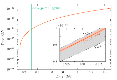
(a)

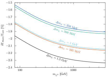
(b)

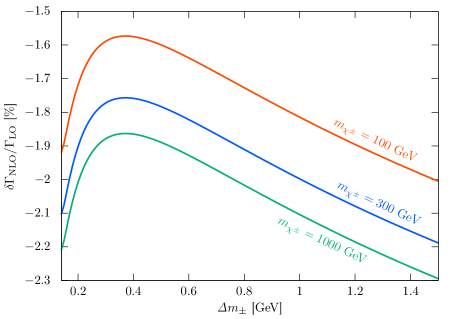
(c)

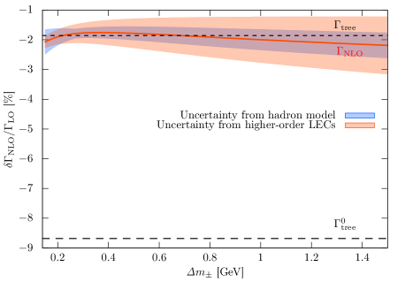
(d)

Figure 10: (a) The NLO decay rate as a function of the mass difference for the 300 GeV charged Higgsino. The inserted window is the close-up view for the mass difference in the limit of the pure Higgsino for $m_{\chi^{\pm}}=300$ GeV, $\mathit{\Delta}m_{\pm}\simeq 310$ MeV. The gray band represents the uncertainties of the tree-level approximation, which is reduced to the very thin orange band at the NLO computation. (b) The ratio of the NLO correction to the leading-order decay rate (6.9) as a function of the chargino mass. (c) The ratio of the NLO correction to the LO decay rate (6.9) as a function of the mass difference. (d) The deviations of $\Gamma_{\mathrm{tree}}$ (6.2), $\Gamma_{\mathrm{tree}}^{0}$ (6.8) and $\Gamma_{\mathrm{NLO}}$ (6.28) from $\Gamma_{\mathrm{LO}}$ (6.9) together with the theoretical uncertainties explained in subsubsection 6.6.3. The NLO single pion decay rate of the Wino can be obtained just by multiplying the result in (a) by four.

In Fig. 10(a), we show the NLO decay rate as a function of the mass difference for the 300 GeV charged Higgsino. The inserted window is the close-up view of the intersection between $\Gamma_{\mathrm{NLO}}$ and the vertical green band, which corresponds to the mass difference of the 300 GeV pure-Higgsino. The gray band represents uncertainty in the tree-level approximation explained in Sec. 6.2; $\Gamma^{0}_{\mathrm{tree}}$ and $\Gamma_{\mathrm{LO}}$ in the figure are given by Eqs. (6.8) and (6.9), respectively. In the close-up window, the NLO decay rate is shown as the orange line accompanied by the very thin light-orange band representing the theoretical error. Fig. 10(b) shows the ratio of the NLO correction to the leading-order decay rate (6.9) as a function of the chargino mass for multiple mass differences. In Fig. 10(c), we show the same ratio as a function of the mass difference for $m_{\chi^{\pm}}=100,300,\mathrm{and}\,1000$ GeV. The figures show that the NLO correction reduces the decay rate from $\Gamma_{\mathrm{LO}}$ by about 2%.

In Fig. 10(d), we show deviations of $\Gamma_{\mathrm{tree}}$ (6.2), $\Gamma_{\mathrm{tree}}^{0}$ (6.8), and $\Gamma_{\mathrm{NLO}}$ (6.28) from $\Gamma_{\mathrm{LO}}$ (6.9) together with the theoretical uncertainties explained in subsubsection 6.6.3 for the 300 GeV Higgsino. The orange band represents theoretical error from the minimal resonance model described by Eqs. (6.83) and (6.84). The blue band indicates uncertainty due to contributions from operators with derivatives on the Higgsinos which are not included in our analysis. The former error is dominated by the latter one for $\mathit{\Delta}m_{\pm}\gtrsim 0.4\,\mathrm{GeV}$. The combined uncertainty of the NLO analysis is a few percent for the mass difference less than 1.5 GeV. Compared with the uncertainty in the “tree-level” estimation of about 9%, i.e. the difference between $\Gamma_{\mathrm{tree}}^{0}$ and $\Gamma_{\mathrm{LO}}$, the NLO analysis substantially reduces the uncertainty of the chargino decay rate into the single pion.

7 Decay into Single Kaon and Multi-Meson

When the mass difference $\mathit{\Delta}m_{\pm}$ exceeds roughly 0.5 GeV, the branching fractions of the chargino decay into a single Kaon as well as multi-meson become significant. For such a large mass difference, the hadron resonances such as the $\rho$-mesons play significant roles. In the following analysis, instead of relying on hadron models, we make use of an observed differential decay rate of the tau lepton to calculate the hadronic chargino decay width. These methods are discussed in Refs. [24]. We revisit these estimations by considering short-distance corrections from electroweak interactions and by using updated data for the hadronic tau lepton decay. These effects result in a difference of several tens of percent from the previous estimations.

7.1 Inclusive Decay Rates

Let us consider a generic decay process, $\chi^{-}(p_{1})\rightarrow\chi^{0}(p_{2})+\mathrm{mesons}$. Here, $p_{1(2)}$ is the momentum of the chargino (neutralino). At tree level, the decay amplitude is given by

$$\mathcal{M}(\chi^{-}\rightarrow\chi^{0}+\mathrm{mesons}) =-2G_{F}V^{*}_{uD}\,\bar{u}_{\chi^{0}}(p_{2})\gamma^{\mu}\quantity(O^{W}_{L}P_{L}+O^{W}_{R}P_{R})u_{\chi^{-}}(p_{1})\matrixelement{\mathrm{mesons}}{U_{\mu}(0)}{0}\ ,$$ (7.1)

where $V_{uD}(D=d,s)$ is the CKM matrix element, and $U_{\mu}(x)$ is the vector $\quantity(U_{\mu}=V_{\mu}=\overline{\Psi}_{D}\gamma^{\mu}\Psi_{u})$ or axial $\quantity(U_{\mu}=A_{\mu}=\overline{\Psi}_{D}\gamma^{\mu}\gamma_{5}\Psi_{u})$ color-singlet quark current. With the spectral functions $v_{J}(s)$ and $a_{J}(s)\,(J=0,1)$ [53], we can write the decay rate into vector ($V^{-}_{J}$) or axial ($A^{-}_{J}$) channel as

$$\Gamma_{\mathrm{tree}}(\chi^{-}\rightarrow\chi^{0}+(V/A)^{-}_{J})= \,\frac{G_{F}^{2}\absolutevalue{V_{uD}}^{2}}{(2\pi)^{3}}\int ds\,\frac{s^{3}}{m_{\chi^{\pm}}^{3}}\lambda_{\chi^{\pm}\chi^{0}}^{1/2}(s)\times(v/a)_{J}(s)K_{J}(s)\ ,$$ (7.2)

where $s=(p_{1}-p_{2})^{2}$ is the invariant mass of the multi-meson system in the final state. For the normalization of the spectral functions, see Appendix D. The kinematical function $\lambda_{AB}(s)$ is given by

$$\lambda_{AB}(s) =\lambda(1,m_{A}^{2}/s,m_{B}^{2}/s)\ ,$$ (7.3)

with $\lambda(a,b,c)=a^{2}+b^{2}+c^{2}-2ab-2bc-2ca$, and

$$K_{J=1}(s)=\frac{1}{2}\left\{-6(O^{W}_{L}O^{W*}_{R}+O^{W*}_{L}O^{W}_{R})\frac{m_{\chi^{0}}m_{\chi^{\pm}}}{s}\phantom{\quantity[-\quantity(\frac{m_{\chi^{\pm}}^{2}-m_{\chi^{0}}^{2}}{s})^{2}]}\right.$$ (7.4)

$$\left.\hskip 120.0pt+\quantity(\absolutevalue{O^{W}_{L}}^{2}+\absolutevalue{O^{W}_{R}}^{2})\quantity[\frac{m_{\chi^{\pm}}^{2}+m_{\chi^{0}}^{2}}{s}-2+\quantity(\frac{m_{\chi^{\pm}}^{2}-m_{\chi^{0}}^{2}}{s})^{2}]\right\}\ ;$$ (7.5)

$$K_{J=0}(s)=\frac{1}{2}\left\{2(O^{W}_{L}O^{W*}_{R}+O^{W*}_{L}O^{W}_{R})\frac{m_{\chi^{0}}m_{\chi^{\pm}}}{s}\phantom{\quantity[-\frac{m_{\chi^{\pm}}^{2}+m_{\chi^{0}}^{2}}{s}+\quantity(\frac{m_{\chi^{\pm}}^{2}-m_{\chi^{0}}^{2}}{s})^{2}]}\right.$$ (7.6)

$$\left.\hskip 120.0pt+\quantity(\absolutevalue{O^{W}_{L}}^{2}+\absolutevalue{O^{W}_{R}}^{2})\quantity[-\frac{m_{\chi^{\pm}}^{2}+m_{\chi^{0}}^{2}}{s}+\quantity(\frac{m_{\chi^{\pm}}^{2}-m_{\chi^{0}}^{2}}{s})^{2}]\right\}\ .$$ (7.7)

The spectral functions $v_{J}(s)$ and $a_{J}(s)$ encapsulate the hadronization effects. In our analysis, we will use the spectral functions obtained from the data of the tau lepton decay up to $s=m_{\tau}^{2}\simeq 3\,\mathrm{GeV}^{2}$. The specific extraction procedure will be detailed in subsections 7.3 and 7.4.

We approximate the electroweak and short-distance QED corrections above $\mu_{\mathrm{IR}}$ by multiplying the tree-level decay rate (7.2) by the factor $S_{\mathrm{EW}}^{\chi}(\mu_{\mathrm{IR}})$ (4.28), with the central value of $\mu_{\mathrm{IR}}$ chosen to be the $\rho$ meson mass. That is, the NLO decay rate is given by

$$\Gamma_{\mathrm{tree+EW}}(\chi^{-}\rightarrow\chi^{0}+(V/A)^{-}_{J})=\Gamma_{\mathrm{tree}}(\chi^{-}\rightarrow\chi^{0}+(V/A)^{-}_{J})\times S_{\mathrm{EW}}^{\chi}(\mu_{\mathrm{IR}}=m_{\rho})\ .$$ (7.8)

This approximation effectively captures the leading logarithmic enhancements in QED. Additionally, it accounts for electroweak corrections that are enhanced by the inverse power of $s_{W}^{2}$. Relative to other sources of theoretical and experimental errors, such as those arising from spectral functions, the remaining non-logarithmic QED corrections are comparatively negligible.

7.2 Single Kaon Mode

The spectral function $a_{0}(s)$ corresponds to $J^{P}=0^{-}$ transitions, and therefore includes the pole of a single meson $P^{-}=\pi^{-},K^{-}$ as

$$a_{0}(s)\supset a_{0}^{P}(s)=\quantity(2\pi F_{P})^{2}\delta(s-m_{P}^{2})\ .$$ (7.9)

Plugging this into Eq. (7.2), we obtain the decay rate of the single meson mode,

$$\Gamma_{\mathrm{tree}}\quantity(\chi^{-}\to\chi^{0}+P^{-})= \frac{F_{P}^{2}G_{F}^{2}\absolutevalue{V_{uD}}^{2}}{8\pi m_{\chi^{\pm}}}\sqrt{\lambda\quantity(1,m_{\chi^{0}}^{2}/m_{\chi^{\pm}}^{2},m_{P}^{2}/m_{\chi^{\pm}}^{2})}$$ (7.10)

$$\times\Bigg{\{}\absolutevalue{O^{W}_{L}+O^{W}_{R}}^{2}\quantity(m_{\chi^{\pm}}-m_{\chi^{0}})^{2}\quantity[\quantity(m_{\chi^{\pm}}+m_{\chi^{0}})^{2}-m_{P}^{2}]$$ (7.11)

$$\hskip 40.0pt+\absolutevalue{O^{W}_{L}-O^{W}_{R}}^{2}\quantity(m_{\chi^{\pm}}+m_{\chi^{0}})^{2}\quantity[\quantity(m_{\chi^{\pm}}-m_{\chi^{0}})^{2}-m_{P}^{2}]\Bigg{\}}\ ,$$ (7.12)

which reproduces the result of the single pion mode (6.2).

We define the leading-order rate of the single Kaon mode in terms of the Kaon partial decay rate to the muon as in the case of the single pion mode,

$$\Gamma_{\mathrm{LO}}(\chi^{-}\to\chi^{0}+K^{-}):=B\quantity(K^{-}\to\mu^{-}+\overline{\nu_{\mu}}(+\gamma))\times\Gamma_{K}^{\mathrm{tot}}\times\frac{\Gamma_{\mathrm{tree}}(\chi^{-}\to\chi^{0}+K^{-})}{\Gamma_{\mathrm{tree}}\quantity(K^{-}\to\mu^{-}+\overline{\mu_{\nu}})}\ ,$$ (7.13)

where $\Gamma^{\mathrm{tot}}_{K}$ is the total decay rate of the charged pion and $B(K^{-}\to\mu^{-}+\overline{\nu_{\mu}}(+\gamma))$ is the branching fraction of the $K_{\mu 2(\gamma)}$ decay. We use measured values for both of $\Gamma_{K}^{\mathrm{tot}}=\tau_{K}^{-1}$ and $B(K^{-}\to\mu^{-}+\overline{\nu_{\mu}}(+\gamma))$ in Table 1.

We approximate the electroweak and short-distance QED corrections to $\Gamma_{\mathrm{LO}}$ as

$$\Gamma_{\mathrm{LO+EW}}(\chi^{-}\to\chi^{0}+K^{-})=\Gamma_{\mathrm{LO}}(\chi^{-}\to\chi^{0}+K^{-})\times S_{\mathrm{EW}}^{\chi\to K}(\mu_{\mathrm{IR}}=m_{\rho})\ ,$$ (7.14)

where 

$$S_{\mathrm{EW}}^{\chi\to K}(\mu_{\mathrm{IR}}):=S_{\mathrm{EW}}^{\chi}(\mu_{\mathrm{IR}})-\frac{\alpha}{4\pi}\cdot 8\log\frac{m_{Z}}{\mu_{\mathrm{IR}}}\ .$$ (7.15)

In the single Kaon mode, we do not compute the long-distance radiative correction, and hence it provides theoretical uncertainty of the decay rate. For the single pion mode, the long-distance NLO correction provides around $3\%$ modification of the leading-order decay rate (6.75). We take this percentage as a crude estimate of the size of the long-distance correction to the single Kaon mode.

7.3 Non-Strange Multi-Meson Modes

Let us consider multi-meson modes without strangeness, e.g., $\pi^{-}\pi^{0}$, $K^{-}K^{0}$, $\pi^{-}2\pi^{0}$, $\pi^{+}2\pi^{-}$, $4\pi$,  $\cdots$ modes. Here, $K^{0}$ is the linear combination of the mass eigenstates $K_{L}$ and $K_{S}$, i.e., $\ket{K_{0}}\simeq(\ket{K_{L}}+\ket{K_{S}})/\sqrt{2}$. For these modes, the relevant spectral functions are $v_{1}(s)/a_{1}(s)$, which can be extracted from the observation of the tau lepton decay based on the relation

$$v_{1}(s)/a_{1}(s) =\frac{m_{\tau}^{2}}{6\absolutevalue{V_{ud}}^{2}S_{\mathrm{EW}}^{\tau}}\frac{B\quantity(\tau^{-}\to V^{-}/A^{-}\nu_{\tau})}{B\quantity(\tau^{-}\to e^{-}\overline{\nu_{e}}\nu_{\tau})}\frac{dN_{V/A}}{N_{V/A}ds}\quantity[\quantity(1-\frac{s}{m_{\tau}^{2}})^{2}\quantity(1+\frac{2s}{m_{\tau}^{2}})]^{-1}\ .$$ (7.16)

Here, $S_{\mathrm{EW}}^{\tau}$ is the short-distance NLO correction defined by Eq. (7.17), $B(\cdots)$ is the branching fraction, and $(1/N_{V/A})dN_{V/A}/ds$ is the normalized invariant mass-distribution from the tau lepton decay. The effect of short- and long-distance corrections to the extraction of these spectral functions will be also discussed below.

7.3.1 Effects of Radiative Corrections to Tau Decay

The short-distance corrections to the hadronic tau lepton decay introduce about 2% modification to the spectral functions. Therefore, it is important to exercise caution when deducing the spectral function from an experimentally measured mass distribution.

The factor $S_{\mathrm{EW}}^{\tau}$ in Eq. (7.16) is given by the ratio between the radiative corrections to the hadron mode and those to the lepton mode of the tau lepton decay,

$$S_{\mathrm{EW}}^{\tau}=\frac{S^{\tau}(m_{\tau},m_{Z})}{\left.S^{\tau}_{\mathrm{EW}}\right|_{\mathrm{lepton}}}\ .$$ (7.17)

Here, the numerator is defined to be the short-distance correction to the hadronic tau lepton decay [54],

$$S^{\tau}(m_{\tau},m_{Z})=\,\, \quantity[\frac{\alpha(m_{b})}{\alpha(m_{\tau})}]^{9/19}\quantity[\frac{\alpha(m_{W})}{\alpha(m_{b})}]^{9/20}\quantity[\frac{\alpha(m_{Z})}{\alpha(m_{W})}]^{36/17}$$ (7.18)

$$\times\quantity[\frac{\alpha_{s}(m_{b})}{\alpha_{s}(m_{\tau})}]^{(3/25)\quantity(\alpha(m_{\tau})/\pi)}\quantity[\frac{\alpha_{s}(m_{Z})}{\alpha_{s}(m_{b})}]^{(3/23)\quantity(\alpha(m_{\tau})/\pi)}$$ (7.19)

$$\simeq\,\, 1.01907\ ,$$ (7.20)

where leading-logarithmic corrections with perturbative QCD effects are resummed. The denominator $\left.S^{\tau}_{\mathrm{EW}}\right|_{\mathrm{lepton}}$ represents the short- and long-distance radiative corrections to the semi-leptonic decay of tau lepton [55, 33],

$$\left.S^{\tau}_{\mathrm{EW}}\right|_{\mathrm{lepton}}=1+\frac{\alpha(m_{\tau})}{4\pi}\quantity(\frac{25}{2}-2\pi^{2})\simeq 0.9957\ ,$$ (7.21)

where no logarithmic enhanced terms appear. Hence, we obtain

$$S_{\mathrm{EW}}^{\tau}=\frac{S^{\tau}(m_{\tau},m_{Z})}{\left.S^{\tau}_{\mathrm{EW}}\right|_{\mathrm{lepton}}}\simeq 1.0235\pm 0.0003\ ,$$ (7.22)

where the error $\pm 0.0003$ incorporates the RG effects [56].

The formula for the spectral functions (7.16) also receives long-distance virtual/real photon corrections to the hadronic tau decay, which depend on what kind of hadrons are in the final state. These effects can be encapsulated by a mode-dependent function $G_{\mathrm{EM}}^{\tau}(s)$ , and the relation of the spectral functions to observed mass distributions should be corrected as

$$v_{1}(s)/a_{1}(s) =\frac{m_{\tau}^{2}}{6\absolutevalue{V_{ud}}^{2}S_{\mathrm{EW}}^{\tau}G_{\mathrm{EM}}^{\tau}(s)}\frac{B\quantity(\tau^{-}\to V^{-}/A^{-}\nu_{\tau})}{B\quantity(\tau^{-}\to e^{-}\overline{\nu_{e}}\nu_{\tau})}\frac{dN_{V/A}}{N_{V/A}ds}\quantity[\quantity(1-\frac{s}{m_{\tau}^{2}})^{2}\quantity(1+\frac{2s}{m_{\tau}^{2}})]^{-1}\ .$$ (7.23)

When representing hadronic chargino decay rates with the spectral functions defined by Eq. (7.23), long-distance corrections to the chargino decay can also be factorized into a similar function $G_{\mathrm{EM}}^{\chi}(s)$. The difference between $G_{\mathrm{EM}}^{\chi}(s)$ and $G_{\mathrm{EM}}^{\tau}(s)$ for each hadronic decay mode would be approximated as

$$\frac{G_{\mathrm{EM}}^{\chi}(s)}{G_{\mathrm{EM}}^{\tau}(s)}-1\simeq O\quantity(\frac{\alpha}{\pi}\log\frac{m_{\tau}}{m_{\pi^{\pm}}})\ ,$$ (7.24)

where we expect that no enhanced corrections of $O((\alpha/\pi)\log m_{\chi^{\pm}})$ appear as we have confirmed in the cases of the leptonic and the single pion modes. In the following analysis, we define the spectral functions by Eq. (7.23) and multiply the decay rate by $G_{\mathrm{EM}}^{\chi}(s)$ for each multi-meson mode. We take $\pm(\alpha/\pi)\log(m_{\tau}/m_{\pi^{\pm}})=\pm 0.6\%$ as the theoretical error for this approximation. Note that the uncertainty from the choice of the IR cutoff $\mu_{\mathrm{IR}}$ in the correction factor (4.28) is replaced by the uncertainty from the long-distance correction $G_{\mathrm{EM}}^{\chi}(s)/G_{\mathrm{EM}}^{\tau}(s)$.

7.3.2 Two-Pion Mode

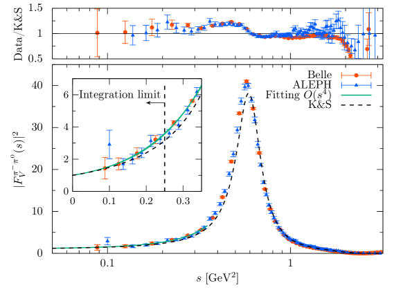
Figure 11: The pion form factor $|F^{\pi^{-}\pi^{0}}_{V}(s)|^{2}$ measured by ALEPH and Belle experiments. The black-dashed line represents the fitting given by Kühn&Santamaria (K&S) [62]. The green band in the close-up window is our fitting with Eq. (7.26). In estimation of the decay rate, we apply the cubic polynomial approximation (7.26) up to the integration limit, $s=0.25\,\mathrm{GeV}^{2}$. Above this limit, we use the linear interpolation of the ALEPH data. The upper panel shows the ratio between the observed data and the K&S fitting curve.

Let us consider the two-pion mode, which is dominant among the multi-meson modes and mediated only by the vector-current. The axial current contribution to the two-pion mode is suppressed by the conservation of $G$-parity. The two-pion part of the spectral function $v_{1}(s)$ (7.16) is related to the pion form factor $F_{V}^{\pi^{-}\pi^{0}}(s)$

$$v_{1}(s)\supset v^{\pi^{-}\pi^{0}}_{1}(s) =\frac{1}{12}\lambda^{3/2}_{\pi^{-}\pi^{0}}(s)\absolutevalue{F^{\pi^{-}\pi^{0}}_{V}(s)}^{2}\ .$$ (7.25)

In our analysis, the numerical estimation of the pion form factor $\absolutevalue{F_{V}^{\pi^{-}\pi^{0}}(s)}^{2}$ is obtained as follows. The pion form factor can be measured by decay of the tau lepton. Following Ref. [63], we fit the experimental data on the pion form factor obtained by the ALEPH [64, 65, 66] and Belle [56] in the range of $s\in[(m_{\pi^{0}}+m_{\pi^{\pm}})^{2},0.35\,\mathrm{GeV}^{2}]$ with

$$F^{\pi^{-}\pi^{0}}_{V}(s)=1+\frac{1}{6}\langle r^{2}\rangle_{\pi}s+c_{1}s^{2}+c_{2}s^{3}+O(s^{4})\ .$$ (7.26)

Here, we use the pion charge radius $\langle r^{2}\rangle_{\pi}$ given by the PDG value [27], $\langle r^{2}\rangle_{\pi}=0.434\pm 0.005\,\mathrm{fm}^{2}$, by assuming the isospin symmetry. In the integration in Eq. (7.2), we apply this cubic polynomial approximation to the form factor up to the integration limit, $s=0.25\,\mathrm{GeV}^{2}$. Above this limit, we use the linear interpolation of the ALEPH data  in Eq. (7.2).

In Fig. 11, we show the observed data [56, 66] of the pion form factor $\absolutevalue{F_{V}^{\pi^{-}\pi^{0}}(s)}^{2}$ together with the fitting curve by the Kühn & Santamaria (K&S) model [62] in the black-dashed line. Here, the parameters of the K&S model are chosen according to the analysis by CDG. The figure shows the observed data is about 10%–20% larger than the K&S fitting curve around $s=0.2$–$0.6$ GeV².

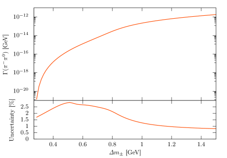
(a)

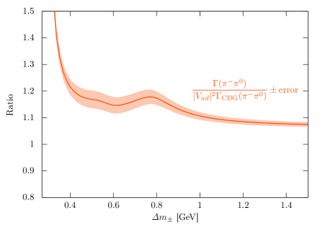
(b)

Figure 12: (a) The partial decay rate and the uncertainty of the two-pion mode for $300\,$GeV Higgsino. (b) The ratio of the decay rates of the two pion mode in the present analysis and that of CDG for $300\,$GeV Higgsino multiplied by $|V_{ud}|^{2}$.

In Fig. 12(a), we show the partial decay rate and its uncertainty of the two-pion mode for the $300\,$GeV Higgsino. The uncertainty comprises errors in data of the pion form factor and the errors from the long-distance NLO correction to the chargino decay, $G_{\mathrm{EM}}^{\chi}(s)/G_{\mathrm{EM}}^{\tau}(s)$. The figure shows that for $\mathit{\Delta}m_{\pm}\simeq 0.5$ GeV, the error of the measured data dominates and provides about 3% uncertainty to the decay rate. For a larger mass difference, e.g. $\mathit{\Delta}m_{\pm}\simeq 1.4$ GeV, the error is dominated by that of the long-distance NLO corrections.

In Fig. 12(b), we compare our numerical result of the chargino decay rate into the two pions with the previous estimate by CDG. Here, we have multiplied the CDG decay rate by the CKM factor $\absolutevalue{V_{ud}}^{2}$, which has not been included in the original expression by CDG. The red band around the ratio corresponds to the error of our analysis. Typically, our estimate is $O(10\%)$ larger than the previous one.

7.3.3 Other Non-Strange Multi-Meson Modes

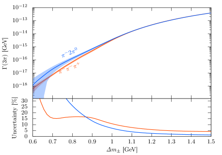
(a)

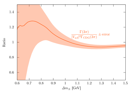
(b)

Figure 13: (a) The partial decay rate and the uncertainty of the three-pion modes for $300\,$GeV Higgsino. (b) The ratio of the decay rates of the three pion modes in the present analysis and that of CDG for $300\,$GeV Higgsino multiplied by $|V_{ud}|^{2}$.

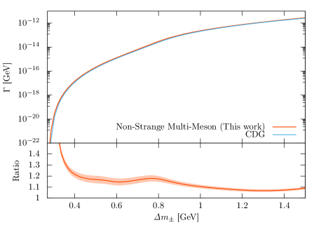
(a)

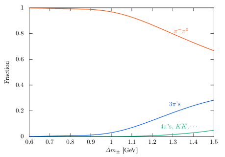
(b)

Figure 14: (a) The decay rate and the uncertainty of the non-strange multi-meson modes for the $300\,$GeV Higgsino. The bottom panel shows the ratio of the decay rates of the non-strange multi-meson modes in the present analysis and that of CDG including $|V_{ud}|^{2}$. (b) The branching fractions of each mode for the 300 GeV Higgsino.

When the mass difference is greater than about 1 GeV, the three-pion modes also provide significant contribution to the chargino decay. We use the linear interpolation of the ALEPH data of the three pion modes to obtain the spectral functions, $a_{1}^{\pi^{+}2\pi^{-}}(s)$ and $a_{1}^{\pi^{-}2\pi^{0}}(s)$. Again, the contribution of $v_{1}(s)$ to the three-pion modes is negligible due to the $G$-parity conservation. In Fig. 13(a), we show the chargino decay rates into three pions and their uncertainties. These uncertainties include both experimental error of the ALEPH data and theoretical error from $G_{\mathrm{EM}}$ (7.24). In the low mass difference, the error of the three-pion modes is dominated by the experimental uncertainty of the ALEPH data. This large uncertainty scarcely affects the estimation of the total chargino decay rate due to their small branching fractions. In Fig. 13(b), we compare our numerical result of the chargino decay rate into three pions with the previous estimate by CDG.

We also include other minor non-strange multi-meson modes, $K^{-}K^{0}$, $4\pi$, $\cdots$, which have not been included in the CDG analysis. In Fig. 14, we summarize non-strange multi-meson modes of the chargino decay with comparison to the previous CDG decay rate. Compared to the previous estimate by CDG, the total rate of the non-strange multi-meson modes increases by about 10%.

7.4 Multi-Meson Modes with Strangeness

There are multi-meson modes with the strangeness final states $\mathit{\Delta}S=-1$. Those modes are suppressed by the Cabbibo angle $V_{us}$, and they provide a few percent contribution to the total decay rate for a larger mass difference.

7.4.1 $\quantity(K\pi)^{-}$ Mode

The form factors for the $\pi^{-}{K}_{S}$ mode are provided by Ref. [56] in the Breit-Wigner approximation,

$$F_{V}^{\pi^{-}K_{S}}(s) =\frac{1}{1+\beta}\quantity[BW_{K^{*}(892)}^{J=1}(s)+\beta BW_{K^{*}(1410)}^{J=1}(s)]\ ;$$ (7.27)

$$F_{S}^{\pi^{-}K_{S}}(s) =\kappa\frac{s}{M_{K^{*}_{0}(800)}}BW_{K^{*}_{0}(800)}^{J=0}(s)\ .$$ (7.28)

Here, $BW_{R}^{J}(s)$ is the Breit-Wigner function for resonance $R$ with mass $M_{R}$,

$$BW_{R}^{J}(s)=\frac{M_{R}^{2}}{s-M_{R}^{2}+i\sqrt{s}\,\Gamma_{R}^{J}(s)}\ .$$ (7.29)

The $s$-dependent total width $\Gamma_{R}(s)$ is given by

$$\Gamma_{R}^{J}(s)=\Gamma_{0R}\frac{M_{R}^{2}}{s}\quantity(\frac{P(s)}{P(M_{R}^{2})})^{2J+1}\ ,$$ (7.30)

where $\Gamma_{0R}$ is the resonance width at its peak, $P(x)$ is given by

$$P(x)=\frac{1}{2\sqrt{x}}\sqrt{\quantity[x-(m_{K}+m_{\pi^{\pm}})^{2}]\quantity[x-(m_{K}-m_{\pi^{\pm}})^{2}]}\ ,$$ (7.31)

and $J=0,1$ is the angular momentum of the $(K\pi)^{-}$ system. Following Ref. [56], we adopt the parameters such as $\beta$ and $\kappa$ fitted in the model including $K_{0}^{*}(800)$, $K^{*}(892)$, and $K^{*}(1410)$ resonances.

These form factors can be translated into the spectral functions in the following relations:

$$v^{\pi^{-}K_{S}}_{1}(s) =\frac{1}{48}\quantity{\frac{2P(s)}{\sqrt{s}}}^{3}\absolutevalue{F^{\pi^{-}K_{S}}_{V}(s)}^{2}\ ;$$ (7.32)

$$v^{\pi^{-}K_{S}}_{0}(s) =\frac{1}{16}\quantity(\frac{m_{K}^{2}-m_{\pi^{\pm}}^{2}}{s})^{2}\,\frac{2P(s)}{\sqrt{s}}\absolutevalue{F^{\pi^{-}K_{S}}_{S}(s)}^{2}\ ;$$ (7.33)

$$v^{\pi^{0}K^{-}}_{1}(s) =v^{\pi^{-}K_{L}}_{1}(s)=v^{\pi^{-}K_{S}}_{1}(s)\ ;\quad v^{\pi^{0}K^{-}}_{0}(s)=v^{\pi^{-}K_{L}}_{0}(s)=v^{\pi^{-}K_{S}}_{0}(s)\ ,$$ (7.34)

where we have used the isospin symmetry. By substituting these spectral functions into Eq. (7.2), we obtain the decay rate into the final state indicated by the superscript of the vector spectral functions.

7.4.2 Other Multi-Meson Modes with Strangeness

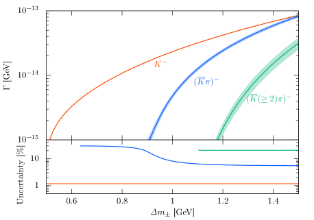
(a)

(b)

Figure 15: The strange hadronic decay modes for the 300 GeV Higgsino. (a) The decay rates and uncertainties of the single $K^{-}$, $\quantity(\overline{K}\pi)^{-}$ and $\quantity(\overline{K}(\geq 2)\pi)^{-}$ modes. (b) The branching ratio of the strange multi-meson modes to the single Kaon mode together with their uncertainties.

The spectral functions for other strange modes such as $\quantity(\overline{K}(\geq 2)\pi)^{-}$ are contained in $v+a$ with $\mathit{\Delta}S=-1$. We approximate the inclusive spectral function by $\left.v+a\right|_{\mathit{\Delta}S=-1}\simeq 1$ which is obtained by the parton model. This approximation is consistent with the observed data of the spectral functions of the strangeness final states. See Fig. 9 in Ref. [67]. To avoid over-counting with the $(K\pi)^{-}$ mode, we include $\left.v+a\right|_{\mathit{\Delta}S=-1}\simeq 1$ contribution only for $s\gtrsim 1.1\,\mathrm{GeV}^{2}$. This treatment reproduces the tau lepton decay rate to $K\,\quantity(\geq 2)\pi$ to accuracy of about $20\%$, and hence the $K\quantity(2\geq)\pi$ modes of the chargino can be predicted to precision of about $20\%$. Since the contributions of the multi-meson modes with the strangeness final states to the total decay rate are minor, this approach provides the level of accuracy necessary for determining the total chargino decay rate as aimed for in this paper.

In Fig. 15, we summarize strange hadronic decay modes for the 300 GeV Higgsino. In Fig. 15(a), we show the decay rates and uncertainties of the single $K^{-}$, $\quantity(\overline{K}\pi)^{-}$ and $\quantity(\overline{K}(\geq 2)\pi)^{-}$ modes. The error of the single Kaon mode is addressed in subsection 7.2. The uncertainty of the $\quantity(\overline{K}\pi)^{-}$ mode comes from that of the experimental data. We estimate the error of $\quantity(\overline{K}(\geq 2)\pi)^{-}$ mode as explained in the previous paragraph. In Fig. 15(b), we show the branching ratio of the strange multi-meson modes to the single Kaon mode together with their uncertainties.

8 Conclusions

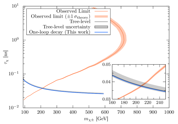
Figure 16: The LHC constraint on the charged Higgsino mass and lifetime based on the disappearing charged track search, where $\mathit{\Delta}m_{\pm}\sim 300$ MeV. The red solid line shows the 95%. limit by the ATLAS with data of $\int\mathcal{L}dt=136\,\mathrm{fb}^{-1}$ and $\sqrt{s}=13$ TeV [19]. The red band shows $\pm 1\,\sigma$ uncertainty of the production cross section of the Higgsino. The upper-left region of the red line has been excluded. The blue solid line is the lifetime based on the NLO decay rate for the pure Higgsino, which decays into $\chi^{0}_{1}$ and $\chi^{0}_{2}$. The gray band shows the tree-level prediction with its uncertainty.

In this paper, we performed precise estimate of the decay rate of the chargino. We extend the previous analysis on the charged Wino decay [23] so as to apply our analysis to larger mass difference between the chargino and the neutralino. We have updated $O(\alpha)$ correction to the single pion mode following the D&M analysis [34] as in the Wino case. Other difference from our previous analysis is in the inclusion of the leptonic mode, the single Kaon mode, and other multi-meson modes. In the leptonic mode, we have computed $O(\alpha)$ corrections with the real emission effects, and predicted the decay rate neglecting of $O(\alpha\mathit{\Delta}m_{\pm}/m_{\chi^{\pm}})$ contributions. We also estimated the single Kaon mode, including the dominant short-distance $O(\alpha)$ corrections, and evaluated the remaining uncertainty by comparison with the single pion case. We also utilized the latest data on hadronic tau lepton decays to estimate the multi-meson decay rates and their associated uncertainties. Through these updates, we achieved the NLO chargino decay rate with a precision of less than 1% for $\mathit{\Delta}m_{\pm}\lesssim 1.5$ GeV. We also emphasize that the NLO results can be applied to the case of more general fermionic electroweak multiplets, e.g., quintuplet dark matter.

As emphasised in the text, the NLO calculation is mandatory to obtain the decay rate with this high precision. In fact, “tree-level” analysis is always subject to indeterminacy due to the choice of tree-level coupling. As we have seen, for example, the choice of either $G_{F}$ or $G_{F}^{0}$ results in the uncertainty of the decay rate about $8$%. Besides, the use of the running gauge coupling constant as the tree-level coupling makes the uncertainty larger.

The reduction of this uncertainty by our NLO analysis plays a critical role in the search for metastable particles at colliders such as the LHC. Fig .16 presents the results from a search using the disappearing charged track technique at the current ATLAS setup. The gray area in the figure underscores the tree-level uncertainty in the pure-Higgsino decay rate, which markedly influences the search for the Higgsinos. As a consequence of this uncertainty, the established mass limit for the Higgsino is subject to a margin of error of approximately 10%. Our one-loop analysis resolved those problems. Currently, a comprehensive two-loop calculation to determine the mass difference of the pure Higgsino is not available. It is anticipated that this gap contributes to an uncertainty in the sub-percent range regarding the mass difference. This uncertainty, in turn, leads to a theoretical prediction of the charged pure Higgsino lifetime with an approximate 1% margin of error. While these theoretical calculations is beyond the scope of this paper, we aim to conduct precise calculations of the mass difference in the near future.

Finally, it should be emphasised that we confirmed that the decay rate becomes independent of $m_{\chi^{\pm}}$ in the limit of $m_{\chi^{\pm}}\to\infty$ at the NLO level. This confirms that the decoupling theorem similar to the Appelquist-Carazzone theorem holds at one-loop level in the chargino decay, although the theorem is not directly applicable to an amplitude where the external lines of the diagrams include heavy particles. We also confirmed that the decay rates of the leptonic and the single pion modes are free from collinear divergences, in accordance with the KLN theorem.

Appendix A Details of Electroweak Corrections

Here, we present the detailed computation of the electroweak corrections to the four-fermion interaction based on the pure-Higgsino Lagrangian (4.2). To see the generalization to other representations of $\mathrm{SU}(2)_{L}\times\mathrm{U}(1)_{Y}$, we introduce a redundant notation of the coupling constants of the fermion $F$ to the $Z$-boson,

$$g_{F}^{Z}=T_{F}^{3}-s_{W}^{2}Q_{F}\ ,$$ (A.1)

where $T^{3}_{F}$ and $Q_{F}$ represent the eigenvalues of the diagonal generator of $\mathrm{SU}(2)_{L}$ and the charge operator with respect to $F$.

A.1 Corrections to Wave-Functions and Vertices

A.1.1 Wave-Function Renormalization of Higgsinos

To begin with, we show the self-energy of the fermions which appear in our problem at one-loop level. We define the self-energy of a fermion with a mass parameter $m_{\mathrm{fermion}}$, which we denote by $\Sigma_{\mathrm{fermion}}(\not{p})$, by the following relation:

$$\Gamma_{\mathrm{fermion}}^{(2)}(p)=(\not{p}-m_{\mathrm{fermion}})-\Sigma_{\mathrm{fermion}}(\not{p})+(\mathrm{CT})\ .$$ (A.2)

Here, $p$ is the momentum of the fermion, $\Gamma^{(2)}_{\mathrm{fermion}}(p)$ is the coefficient of the quadratic term in the quantum effective action, and $(\mathrm{CT})$ represents the wavefunction and the mass counterterm. In the following, we use the dimensional regularization with $d=4-2\epsilon_{\mathrm{EW}}$.

The self-energies provide corrections to a decay amplitude as a residue of external legs. At $O(\alpha)$, the derivatives of $\Sigma(\not{p})$ at the $\mathrm{SU}(2)_{L}$ symmetric mass appear in the amplitude. The virtual $\gamma/Z/W$ contributions to the wave-function of the charged Higgsino are given by

$$\frac{d}{d\not{p}}\Sigma_{-}^{\mathrm{\gamma}}(m_{\chi})=-Q_{\chi^{-}}^{2}\frac{\alpha}{4\pi}\left(\frac{1}{\bar{\epsilon}_{\mathrm{EW}}}+\log\frac{\mu_{\mathrm{EW}}^{2}}{m_{\chi}^{2}}-2\log\frac{m_{\chi}^{2}}{m_{\gamma}^{2}}+4\right)\ ;$$ (A.3)

$$\frac{d}{d\not{p}}\Sigma_{-}^{Z\mathrm{(EW)}}(m_{\chi})=-\frac{1}{c_{W}^{2}s_{W}^{2}}\quantity(g^{Z}_{\chi^{-}})^{2}\frac{\alpha}{4\pi}\left[\frac{1}{\bar{\epsilon}_{\mathrm{EW}}}+\log\frac{\mu_{\mathrm{EW}}^{2}}{m_{\chi}^{2}}+F_{\Sigma}(r_{Z})\right]\ ;$$ (A.4)

$$\frac{d}{d\not{p}}\Sigma_{-}^{W\mathrm{(EW)}}(m_{\chi})=-\quantity(\frac{1}{\sqrt{2}s_{W}})^{2}\frac{\alpha}{4\pi}\left[\frac{1}{\bar{\epsilon}_{\mathrm{EW}}}+\log\frac{\mu_{\mathrm{EW}}^{2}}{m_{\chi}^{2}}+F_{\Sigma}(r_{W})\right]\ .$$ (A.5)

Here, $\mu_{\mathrm{EW}}$ is an arbitrary mass parameter, $\bar{\epsilon}_{\mathrm{EW}}^{-1}=\epsilon_{\mathrm{EW}}^{-1}-\gamma_{E}+\log 4\pi$ with $\gamma_{E}$ being the Euler-Mascheroni constant, and $m_{\gamma}$ a photon mass to regulate the infrared singularity. The function $F_{\Sigma}$ is given by

$$F_{\Sigma}(r)=4\log r+4+3r^{2}-3r^{4}\log r-\frac{3r(4+2r^{2}-r^{4})}{\sqrt{4-r^{2}}}\cos^{-1}\frac{r}{2}\ .$$ (A.6)

The arguments $r_{W}$ and $r_{Z}$ are given by $r_{W}=m_{W}/m_{\chi}$ and $r_{Z}=m_{Z}/m_{\chi}$, respectively.

To avoid confusion in the matching procedure, we label the UV pole and the arbitrary scale with the name of theory which provides them; The pole $\epsilon^{-1}_{\mathrm{EW}}$ means the UV divergence arising from loops in the electroweak theory. Similarly, the subscript of $\mu_{\mathrm{EW}}$ shows that the scale is generated by the dimensional regularization in the electroweak theory.

The normalization of the wave-function of the neutral Higgsino is contributed by the virtual $Z/W$ loops: 

$$\frac{d}{d\not{p}}\Sigma_{0}^{Z\mathrm{(EW)}}(m_{\chi})=-\frac{1}{c_{W}^{2}s_{W}^{2}}\quantity(g^{Z}_{\chi^{0}})^{2}\frac{\alpha}{4\pi}\left[\frac{1}{\bar{\epsilon}_{\mathrm{EW}}}+\log\frac{\mu_{\mathrm{EW}}^{2}}{m_{\chi}^{2}}+F_{\Sigma}(r_{Z})\right]\ ;$$ (A.7)

$$\frac{d}{d\not{p}}\Sigma_{0}^{W\mathrm{(EW)}}(m_{\chi})=-\quantity(\frac{1}{\sqrt{2}s_{W}})^{2}\frac{\alpha}{4\pi}\left[\frac{1}{\bar{\epsilon}_{\mathrm{EW}}}+\log\frac{\mu_{\mathrm{EW}}^{2}}{m_{\chi}^{2}}+F_{\Sigma}(r_{W})\right]\ .$$ (A.8)

The contribution from the wave-function renormalizations of the Higgsinos is given by 

$$\mathcal{M}^{\chi,0}_{\mathrm{WF(EW)}}=\mathcal{M}^{0}_{\mathrm{tree}}\times\quantity[\frac{1}{2}\frac{d}{d\not{p}}\Sigma_{0}^{(\mathrm{EW})}(m_{\chi})+\frac{1}{2}\frac{d}{d\not{p}}\Sigma_{-}^{(\mathrm{EW})}(m_{\chi})]\ ,$$ (A.9)

where

$$\frac{d}{d\not{p}}\Sigma_{0}^{(\mathrm{EW})} =\frac{d}{d\not{p}}\Sigma_{0}^{Z(\mathrm{EW})}+\frac{d}{d\not{p}}\Sigma_{0}^{W(\mathrm{EW})}\ ;$$ (A.10)

$$\frac{d}{d\not{p}}\Sigma_{-}^{(\mathrm{EW})} =\frac{d}{d\not{p}}\Sigma_{-}^{\gamma(\mathrm{EW})}+\frac{d}{d\not{p}}\Sigma_{-}^{Z(\mathrm{EW})}+\frac{d}{d\not{p}}\Sigma_{-}^{W(\mathrm{EW})}\ .$$ (A.11)

A.1.2 Corrections to Vertex of Higgsinos

(a)

(b)

(c)

Figure 17: Radiative corrections to the Higgsino’s vertex.

The Higgsino’s vertex receives the radiative corrections shown in Figs. 17(a)-17(c), which can be written as multiplicative factors to the tree-level amplitude:

$$\mathcal{M}_{\chi}^{Z,0} =\mathcal{M}_{\mathrm{tree}}^{0}\times\frac{g^{Z}_{\chi^{0}}g^{Z}_{\chi^{-}}}{c_{W}^{2}s_{W}^{2}}\frac{\alpha}{4\pi}\quantity[\frac{1}{\bar{\epsilon}_{\mathrm{EW}}}+\log\frac{\mu_{\mathrm{EW}}^{2}}{m_{\chi}^{2}}+F_{\Sigma}\quantity(r_{Z})]\ ;$$ (A.12)

$$\mathcal{M}_{\chi}^{\gamma W,0} =\mathcal{M}_{\mathrm{tree}}^{0}\times\mathit{\Delta}Q_{\chi}\frac{\alpha}{4\pi}\quantity[\frac{3}{\bar{\epsilon}_{\mathrm{EW}}}+3\log\frac{\mu_{\mathrm{EW}}^{2}}{m_{\chi}^{2}}+F_{\chi}^{\gamma W}(r_{W})]\ ;$$ (A.13)

$$\mathcal{M}_{\chi}^{WZ,0} =\mathcal{M}_{\mathrm{tree}}^{0}\times\frac{g^{Z}_{\chi^{0}}-g^{Z}_{\chi^{-}}}{s_{W}^{2}}\frac{\alpha}{4\pi}\quantity[\frac{3}{\bar{\epsilon}_{\mathrm{EW}}}+3\log\frac{\mu_{\mathrm{EW}}^{2}}{m_{\chi}^{2}}+F_{\chi}^{WZ}(r_{W})]\ ,$$ (A.14)

where the $\mathit{\Delta}Q_{\chi}=Q_{\chi^{0}}-Q_{\chi^{-}}=1$ is the charge difference between the neutralino and the chargino, and

$$F_{\chi}^{\gamma W}(r_{W})= \,4+r_{W}^{2}-r_{W}^{4}\log(r_{W})-r_{W}(2+r_{W}^{2})\sqrt{4-r_{W}^{2}}\cot^{-1}\quantity(\frac{r_{W}}{\sqrt{4-r_{W}^{2}}})\,,$$ (A.15)

$$F_{\chi}^{WZ}(r_{W})= \,4+\quantity(1+\frac{1}{c_{W}^{2}})r_{W}^{2}+\frac{\log(c_{W})}{c_{W}^{4}s_{W}^{2}}r_{W}^{4}-\quantity(1+\frac{1}{c_{W}^{2}}+\frac{1}{c_{W}^{4}})r_{W}^{4}\log(r_{W})$$

$$+\frac{c_{W}^{2}}{s_{W}^{2}}(2+r_{W}^{2})r_{W}\sqrt{4-r_{W}^{2}}\cot^{-1}\quantity(\frac{r_{W}}{\sqrt{4-r_{W}^{2}}})$$

$$-\frac{2c_{W}^{2}+r_{W}^{2}}{c_{W}^{4}s_{W}^{2}}r_{W}\sqrt{4c_{W}^{2}-r_{W}^{2}}\cot^{-1}\quantity(\frac{r_{W}}{\sqrt{4c_{W}^{2}-r_{W}^{2}}})\ .$$ (A.16)

Note that the virtual $W$-boson loop does not exist in the corrections to the charged-current operator of the Higgsinos, since we treat the neutral Higgsino as a Dirac fermion.

A.1.3 Renormalization

The virtual $Z$-boson contribution to the charged-current operator of the Higgsinos is given by

$$\mathcal{M}^{Z,0}_{J_{\chi}^{-}} =\mathcal{M}_{\chi}^{Z,0}+\mathcal{M}^{0}_{\mathrm{tree}}\times\quantity[\frac{1}{2}\frac{d}{d\not{p}}\Sigma_{0}^{Z(\mathrm{EW})}(m_{\chi})+\frac{1}{2}\frac{d}{d\not{p}}\Sigma_{-}^{Z(\mathrm{EW})}(m_{\chi})]$$ (A.17)

$$=\mathcal{M}^{0}_{\mathrm{tree}}\times\frac{-\quantity(g^{Z}_{\chi^{0}}-g^{Z}_{\chi^{-}})^{2}}{2c_{W}^{2}s_{W}^{2}}\frac{\alpha}{4\pi}\quantity[\frac{1}{\bar{\epsilon}_{\mathrm{EW}}}+\log\frac{\mu_{\mathrm{EW}}^{2}}{m_{\chi}^{2}}+F_{\Sigma}(r_{Z})]$$ (A.18)

$$=\mathcal{M}^{0}_{\mathrm{tree}}\times\frac{-\quantity(\mathit{\Delta}Q_{\chi})^{2}}{2}\frac{c_{W}^{2}}{s_{W}^{2}}\frac{\alpha}{4\pi}\quantity[\frac{1}{\bar{\epsilon}_{\mathrm{EW}}}+\log\frac{\mu_{\mathrm{EW}}^{2}}{m_{\chi}^{2}}+F_{\Sigma}(r_{Z})]\ .$$ (A.19)

Note that not only the divergent part but also the finite part is independent of the hypercharge thanks to neglecting the momentum transfer. Similarly, the virtual photon/$W$ contribution to the charged-current operator of the Higgsinos is given by

$$\mathcal{M}^{\gamma,0}_{J_{\chi}^{-}} =\mathcal{M}^{0}_{\mathrm{tree}}\times\frac{-\quantity(\mathit{\Delta}Q_{\chi})^{2}}{2}\frac{\alpha}{4\pi}\quantity(\frac{1}{\bar{\epsilon}_{\mathrm{EW}}}+\log\frac{\mu_{\mathrm{EW}}^{2}}{m_{\chi}^{2}}+4-2\log\frac{m_{\chi}^{2}}{m_{\gamma}^{2}})\ ;$$ (A.20)

$$\mathcal{M}^{W,0}_{J_{\chi}^{-}} =\mathcal{M}^{0}_{\mathrm{tree}}\times\frac{-1}{2s_{W}^{2}}\frac{\alpha}{4\pi}\quantity[\frac{1}{\bar{\epsilon}_{\mathrm{EW}}}+\log\frac{\mu_{\mathrm{EW}}^{2}}{m_{\chi}^{2}}+F_{\Sigma}(r_{W})]\ .$$ (A.21)

The total of virtual contributions from the wave-function renormalization and the vertex corrections can be simplified as

$$\left.\mathcal{M}^{\chi,0}_{\mathrm{WF+Vertex(EW)}}\right|_{\mathrm{Virtual}}=\,\, \sum_{V=\gamma,Z,W}\mathcal{M}_{J_{\chi}^{-}}^{V,0}+\mathcal{M}_{\chi}^{\gamma W,0}+\mathcal{M}_{\chi}^{WZ,0}$$ (A.22)

$$=\,\, \left\{\quantity[\frac{2}{s_{W}^{2}}-\frac{(5-\mathit{\Delta}Q_{\chi})(1-\mathit{\Delta}Q_{\chi})}{2s_{W}^{2}}]\quantity(\frac{1}{\bar{\epsilon}_{\mathrm{EW}}}+\log\frac{\mu_{\mathrm{EW}}^{2}}{m_{\chi}^{2}})\right.$$ (A.23)

$$\left.-\frac{1}{2s_{W}^{2}}F_{\Sigma}(r_{W})+\mathit{\Delta}Q_{\chi}\quantity[F_{\chi}^{\gamma W}(r_{W})+\frac{c_{W}^{2}}{s_{W}^{2}}F_{\chi}^{WZ}(r_{W})]\right.$$ (A.24)

$$\left.-\frac{1}{2}\quantity(\mathit{\Delta}Q_{\chi})^{2}\quantity[4-2\log\frac{m_{\chi}^{2}}{m_{\gamma}^{2}}+F_{\Sigma}(r_{Z})]\right\}\times\mathcal{M}^{0}_{\mathrm{tree}}\ .$$ (A.25)

As long as we consider transitions with $\mathit{\Delta}Q_{\chi}=1$, the UV divergence must be canceled with the counterterm determined by the renormalization of the weak gauge coupling and the wave-function of the weak gauge boson because of the gauge invariance. The counterterm contribution is given by

$$\left.\mathcal{M}^{0}_{\mathrm{Vertex}(\mathrm{EW})}\right|_{\mathrm{CT}}=\mathcal{M}^{0}_{\mathrm{tree}}\times(\delta Z_{1}^{W}-\delta Z_{2}^{W})\ ,$$ (A.26)

where $\delta Z_{1}^{W}$ is the renormalization constants of the weak gauge coupling and $\delta Z_{2}^{W}$ is the renormalization factor of the wave function of the weak gauge boson. In the on-shell renormalization scheme of the electroweak theory, this counterterm is set to satisfy [28]

$$\delta Z_{1}^{W}-\delta Z_{2}^{W}=-\frac{2}{s_{W}^{2}}\frac{\alpha}{4\pi}\left(\frac{1}{\bar{\epsilon}_{\mathrm{EW}}}+\log\frac{\mu_{\mathrm{EW}}^{2}}{m_{W}^{2}}\right)\ ,$$ (A.27)

which successfully subtract the UV pole in Eq. (A.22) when $\mathit{\Delta}Q_{\chi}=1$. By combining the counterterm contribution (A.26) with Eq. (A.22), we obtain

$$\mathcal{M}^{\chi,0}_{\mathrm{WF+Vertex(EW)}} =\left.\mathcal{M}^{\chi,0}_{\mathrm{WF+Vertex(EW)}}\right|_{\mathrm{Virtual}}+\left.\mathcal{M}^{0}_{\mathrm{Vertex(EW)}}\right|_{\mathrm{CT}}$$ (A.28)

$$=2\log\frac{m_{W}}{m_{\gamma}}+F^{\mathrm{WF+Vertex(EW)}}_{\chi}(r_{W})\ ,$$ (A.29)

where we have set $\mathit{\Delta}Q_{\chi}=1$ and defined the functions

$$F^{\mathrm{WF+Vertex(EW)}}_{\chi}(r_{W})=\,\, -2+\frac{2c_{W}^{2}}{s_{W}^{2}}\log c_{W}$$ (A.30)

$$-\frac{1}{2s_{W}^{2}}\bar{F}_{\Sigma}(r_{W})-\frac{c_{W}^{2}}{2s_{W}^{2}}\bar{F}_{\Sigma}(r_{Z})+F_{\chi}^{\gamma W}(r_{W})+\frac{c_{W}^{2}}{s_{W}^{2}}F_{\chi}^{WZ}(r_{W})\ ;$$ (A.31)

$$\bar{F}_{\Sigma}(r)=\,\, 4+3r^{2}-3r^{4}\log r-\frac{3r(4+2r^{2}-r^{4})}{\sqrt{4-r^{2}}}\cos^{-1}\frac{r}{2}\ ,$$ (A.32)

which remain finite in the limit of $r\to 0$.

We would like to stress that the coefficients of the amplitudes $\mathcal{M}_{\chi}^{\gamma W,0}$ (A.13), $\mathcal{M}_{\chi}^{WZ,0}$ (A.14), $\mathcal{M}_{J_{\chi}^{-}}^{Z,0}$ (A.17), and $\mathcal{M}_{J_{\chi}^{-}}^{\gamma,0}$ (A.20) are determined only by the charge difference. Given that the cancellation of the UV divergence in Eq. (A.22) by the counterterm contribution (A.26), which is independent of the $\mathrm{SU}(2)_{L}\times\mathrm{U}(1)_{Y}$ representation of the chargino/neutralino multiplet, the coefficient of Eq. (A.21) is also independent of the representation of the decaying particle as long as $\mathit{\Delta}Q_{\chi}=1$.  Consequently, the one-loop contribution from the wave-function and vertex corrections (A.28) does not depend on the representation of the external fermion for the weak transition with $\mathit{\Delta}Q_{\chi}=1$.

A.1.4 Corrections to SM Fermions

The contribution from the wave-function renormalizations and the vertex corrections to the SM fermions can be computed in a similar way. The wave-function renormalization in the SM fermions gives rise to the amplitude,

$$\mathcal{M}_{\mathrm{WF(EW)}}^{f,0}=\mathcal{M}_{\mathrm{tree}}^{0}\times\quantity[\frac{1}{2}\frac{d}{d\not{p}}\Sigma_{f_{L}}^{(\mathrm{EW})}(0)+\frac{1}{2}\frac{d}{d\not{p}}\Sigma_{f^{\prime}_{L}}^{(\mathrm{EW})}(0)]\ ,$$ (A.33)

where for $F=f$ or $f^{\prime}$,

$$\frac{d}{d\not{p}}\Sigma_{F}^{\mathrm{(EW)}}(0)=\frac{d}{d\not{p}}\Sigma_{F}^{\mathrm{\gamma(EW)}}(0)\frac{d}{d\not{p}}\Sigma_{F_{L}}^{\mathrm{Z(EW)}}(0)\frac{d}{d\not{p}}\Sigma_{F_{L}}^{\mathrm{W(EW)}}(0)\ ,$$ (A.34)

and

$$\frac{d}{d\not{p}}\Sigma_{F}^{\mathrm{\gamma(EW)}}(0)=-Q_{F}^{2}\frac{\alpha}{4\pi}\quantity(\frac{1}{\bar{\epsilon}_{\mathrm{EW}}}+\log\frac{\mu_{\mathrm{EW}}^{2}}{m_{\gamma}^{2}}-\frac{1}{2})\ ;$$ (A.35)

$$\frac{d}{d\not{p}}\Sigma_{F_{L}}^{Z\mathrm{(EW)}}(0)=-\frac{1}{c_{W}^{2}s_{W}^{2}}\quantity(g_{F}^{Z})^{2}\frac{\alpha}{4\pi}\quantity(\frac{1}{\bar{\epsilon}_{\mathrm{EW}}}+\log\frac{\mu_{\mathrm{EW}}^{2}}{m_{Z}^{2}}-\frac{1}{2})\ ;$$ (A.36)

$$\frac{d}{d\not{p}}\Sigma_{F_{L}}^{W\mathrm{(EW)}}(0)=-\quantity(\frac{1}{\sqrt{2}s_{W}})^{2}\frac{\alpha}{4\pi}\quantity(\frac{1}{\bar{\epsilon}_{\mathrm{EW}}}+\log\frac{\mu_{\mathrm{EW}}^{2}}{m_{W}^{2}}-\frac{1}{2})\ .$$ (A.37)

(a)

(b)

(c)

Figure 18: Radiative corrections to SM fermion’s vertex.

The radiative corrections to the SM fermion’s vertex (Figs. 18(a)-18(c)) are given by

$$\mathcal{M}^{\gamma,0}_{ff^{\prime}} =\mathcal{M}_{\mathrm{tree}}^{0}\times Q_{f}Q_{f^{\prime}}\frac{\alpha}{4\pi}\left(\frac{1}{\bar{\epsilon}_{\mathrm{EW}}}+\log\frac{\mu_{\mathrm{EW}}^{2}}{m_{\gamma}^{2}}-\frac{1}{2}\right)\ ;$$ (A.38)

$$\mathcal{M}^{Z,0}_{ff^{\prime}} =\mathcal{M}_{\mathrm{tree}}^{0}\times\frac{g_{f}^{Z}g_{f^{\prime}}^{Z}}{c_{W}^{2}s_{W}^{2}}\frac{\alpha}{4\pi}\left(\frac{1}{\bar{\epsilon}_{\mathrm{EW}}}+\log\frac{\mu_{\mathrm{EW}}^{2}}{m_{Z}^{2}}-\frac{1}{2}\right)\ ;$$ (A.39)

$$\mathcal{M}^{\gamma W,0}_{ff^{\prime}} =\mathcal{M}_{\mathrm{tree}}^{0}\times\mathit{\Delta}Q_{f}\frac{\alpha}{4\pi}\left(\frac{3}{\bar{\epsilon}_{\mathrm{EW}}}+3\log\frac{\mu_{\mathrm{EW}}^{2}}{m_{W}^{2}}+\frac{5}{2}\right)\ ;$$ (A.40)

$$\mathcal{M}^{WZ,0}_{ff^{\prime}} =\mathcal{M}_{\mathrm{tree}}^{0}\times\frac{g_{f^{\prime}}^{Z}-g_{f}^{Z}}{s_{W}^{2}}\frac{\alpha}{4\pi}\left(\frac{3}{\bar{\epsilon}_{\mathrm{EW}}}+3\log\frac{\mu_{\mathrm{EW}}^{2}}{m_{W}^{2}}+\frac{5}{2}+\frac{3}{s_{W}^{2}}\log c_{W}^{2}\right)\ ,$$ (A.41)

where we have defined the charge difference $\mathit{\Delta}Q_{f}=Q_{f^{\prime}}-Q_{f}=1$.

From these amplitudes, we obtain the virtual $\gamma/Z/W$ corrections to the charged-current operator composed of the SM fermions,

$$\mathcal{M}_{J_{f}^{-}}^{\gamma,0} =-\frac{\quantity(\mathit{\Delta}Q_{f})^{2}}{2}\frac{\alpha}{4\pi}\left(\frac{1}{\bar{\epsilon}_{\mathrm{EW}}}+\log\frac{\mu_{\mathrm{EW}}^{2}}{m_{\gamma}^{2}}-\frac{1}{2}\right)\times\mathcal{M}_{\mathrm{tree}}^{0}\ ;$$ (A.42)

$$\mathcal{M}_{J_{f}^{-}}^{Z,0} =-\frac{\quantity(g_{f^{\prime}Z}-g_{fZ})^{2}}{2c_{W}^{2}s_{W}^{2}}\frac{\alpha}{4\pi}\left(\frac{1}{\bar{\epsilon}_{\mathrm{EW}}}+\log\frac{\mu_{\mathrm{EW}}^{2}}{m_{Z}^{2}}-\frac{1}{2}\right)\times\mathcal{M}_{\mathrm{tree}}^{0}$$ (A.43)

$$=-\frac{c_{W}^{2}}{s_{W}^{2}}\frac{\quantity(\mathit{\Delta}Q_{f})^{2}}{2}\frac{\alpha}{4\pi}\left(\frac{1}{\bar{\epsilon}_{\mathrm{EW}}}+\log\frac{\mu_{\mathrm{EW}}^{2}}{m_{Z}^{2}}-\frac{1}{2}\right)\times\mathcal{M}_{\mathrm{tree}}^{0}\ ;$$ (A.44)

$$\mathcal{M}_{J_{f}^{-}}^{W,0} =-\frac{1}{2s_{W}^{2}}\frac{\alpha}{4\pi}\left(\frac{1}{\bar{\epsilon}_{\mathrm{EW}}}+\log\frac{\mu_{\mathrm{EW}}^{2}}{m_{W}^{2}}-\frac{1}{2}\right)\times\mathcal{M}_{\mathrm{tree}}^{0}\ .$$ (A.45)

The total of virtual contributions from the wave-function renormalization and the vertex corrections to the SM fermions is given by

$$\left.\mathcal{M}^{f,0}_{\mathrm{WF+Vertex(EW)}}\right|_{\mathrm{Virtual}}=\,\, \sum_{V=\gamma,Z,W}\mathcal{M}_{J_{f}^{-}}^{V,0}+\mathcal{M}_{ff^{\prime}}^{\gamma W,0}+\mathcal{M}_{ff^{\prime}}^{WZ,0}$$ (A.46)

$$=\,\, \left\{\quantity[\frac{2}{s_{W}^{2}}-\frac{(5-\mathit{\Delta}Q_{\chi})(1-\mathit{\Delta}Q_{\chi})}{2s_{W}^{2}}]\quantity(\frac{1}{\bar{\epsilon}_{\mathrm{EW}}}+\log\frac{\mu_{\mathrm{EW}}^{2}}{m_{W}^{2}})\right.$$ (A.47)

$$\left.-\frac{1}{2s_{W}^{2}}\quantity(-\frac{1}{2})+\mathit{\Delta}Q_{f}\quantity[\frac{5}{2}+\frac{c_{W}^{2}}{s_{W}^{2}}\quantity(\frac{5}{2}+\frac{6}{s_{W}^{2}}\log c_{W})]\right.$$ (A.48)

$$\left.-\frac{1}{2}\quantity(\mathit{\Delta}Q_{\chi})^{2}\quantity[\log\frac{m_{W}^{2}}{m_{\gamma}^{2}}-\frac{1}{2}+\frac{c_{W}^{2}}{s_{W}^{2}}\quantity(\log c_{W}-\frac{1}{2})]\right\}\times\mathcal{M}_{\mathrm{tree}}^{0}\ .$$ (A.49)

By combining the counterterm contribution (A.26) with Eq. (A.46), we obtain the UV finite amplitude,

$$\mathcal{M}^{f,0}_{\mathrm{WF+Vertex(EW)}} =\left.\mathcal{M}^{f,0}_{\mathrm{WF+Vertex}}\right|_{\mathrm{Virtual}}+\left.\mathcal{M}^{0}_{\mathrm{Vertex(EW)}}\right|_{\mathrm{CT}}$$ (A.50)

$$=-\log\frac{m_{W}}{m_{\gamma}}+\frac{3}{s_{W}^{2}}+\frac{(6-s_{W}^{2})c_{W}^{2}}{s_{W}^{4}}\log c_{W}\ ,$$ (A.51)

where we have set $\mathit{\Delta}Q_{f}=1$.

A.2 Box Contribution

(a)

(b)

Figure 19: Box contribution from virtual photon.

(a)

(b)

(c)

(d)

Figure 20: Box contributions from virtual $Z$ boson.

The box contributions generated by the virtual photon exchange (Fig 19(a) and 19(b)) can be written in the form:

$$\mathcal{M}_{\mathrm{box},a}^{\gamma\mathrm{(EW)},0} =Q_{f}Q_{\chi^{-}}\frac{\alpha}{4\pi}\quantity{\mathcal{M}_{\mathrm{tree}}^{0}\times\quantity[\log\frac{m_{W}^{2}}{m_{\gamma}^{2}}+F^{\gamma\mathrm{(EW)}}_{V}(r_{W})]+\mathcal{M}_{A}^{0}\times F^{\gamma\mathrm{(EW)}}_{A}(r_{W})}\ ;$$ (A.52)

$$\mathcal{M}_{\mathrm{box},b}^{\gamma\mathrm{(EW)},0} =Q_{f^{\prime}}Q_{\chi^{-}}\frac{\alpha}{4\pi}\quantity{-\mathcal{M}_{\mathrm{tree}}^{0}\times\quantity[\log\frac{m_{W}^{2}}{m_{\gamma}^{2}}+F^{\gamma\mathrm{(EW)}}_{V}(r_{W})]+\mathcal{M}_{A}^{0}\times F^{\gamma\mathrm{(EW)}}_{A}(r_{W})}\ ,$$ (A.53)

where $\mathcal{M}_{A}^{0}$ is the axial current contribution given by Eq. (4.16) and

$$F^{\gamma\mathrm{(EW)}}_{V}(r_{W}) =-\frac{r_{W}^{2}}{2}+\frac{1}{2}r_{W}^{4}\log(r_{W})+r_{W}\quantity(1+\frac{r_{W}^{2}}{2})\sqrt{4-r_{W}^{2}}\cot^{-1}\quantity(\frac{r_{W}}{\sqrt{4-r_{W}^{2}}})\ ;$$ (A.54)

$$F^{\gamma\mathrm{(EW)}}_{A}(r_{W}) =\frac{r_{W}}{6}\left[-r_{W}+r_{W}(6+r_{W}^{2})\log(r_{W})+(8+r_{W}^{2})\sqrt{4-r_{W}^{2}}\cot^{-1}\quantity(\frac{r_{W}}{\sqrt{4-r_{W}^{2}}})\right]\ .$$ (A.55)

Hence, the photon box contribution can be summarized as

$$\mathcal{M}_{\mathrm{box}}^{\gamma,0}=\mathcal{M}_{\mathrm{tree}}^{0}\times\mathit{\Delta}Q_{\chi}\mathit{\Delta}Q_{f}\frac{\alpha}{4\pi}\quantity[\log\frac{m_{W}^{2}}{m_{\gamma}^{2}}+F^{\gamma\mathrm{(EW)}}_{V}(r_{W})]-\mathcal{M}_{A}^{0}\times\overline{Q}\frac{\alpha}{4\pi}F^{\gamma\mathrm{(EW)}}_{A}(r_{W})\ ,$$ (A.56)

where $\overline{Q}=Q_{f}+Q_{f^{\prime}}$. The coefficient of the vector-like part depends only on the charge differences, and hence, is independent of the representation of the chargino/neutralino multiplet.

$Z$-boson exchanges generate the box diagrams depicted in Figs. 20(a)$-$20(d), which have contributions given by

$$\mathcal{M}^{Z\mathrm{(EW)},0}_{\mathrm{box},a}=\, \frac{g_{\chi^{-}}^{Z}g_{f}^{Z}}{4c_{W}^{4}s_{W}^{4}}\frac{\alpha}{4\pi}\quantity[\mathcal{M}_{\mathrm{tree}}^{0}\times F^{Z\mathrm{(EW)}}_{V}(r_{W})+\mathcal{M}_{A}^{0}\times F^{Z\mathrm{(EW)}}_{A}(r_{W})]\ ;$$ (A.57)

$$\mathcal{M}^{Z\mathrm{(EW)},0}_{\mathrm{box},b}=\, \frac{g_{\chi^{-}}^{Z}g_{f^{\prime}}^{Z}}{4c_{W}^{4}s_{W}^{4}}\frac{\alpha}{4\pi}\quantity[-\mathcal{M}_{\mathrm{tree}}^{0}\times F^{Z\mathrm{(EW)}}_{V}(r_{W})+\mathcal{M}_{A}^{0}\times F^{Z\mathrm{(EW)}}_{A}(r_{W})]\ ;$$ (A.58)

$$\mathcal{M}^{Z\mathrm{(EW)},0}_{\mathrm{box},c}=\, \frac{g_{\chi^{0}}^{Z}g_{f}^{Z}}{4c_{W}^{4}s_{W}^{4}}\frac{\alpha}{4\pi}\quantity[-\mathcal{M}_{\mathrm{tree}}^{0}\times F^{Z\mathrm{(EW)}}_{V}(r_{W})+\mathcal{M}_{A}^{0}\times F^{Z\mathrm{(EW)}}_{A}(r_{W})]\ ;$$ (A.59)

$$\mathcal{M}^{Z\mathrm{(EW)},0}_{\mathrm{box},d}=\, \frac{g_{\chi^{0}}^{Z}g_{f^{\prime}}^{Z}}{4c_{W}^{4}s_{W}^{4}}\frac{\alpha}{4\pi}\quantity[\mathcal{M}_{\mathrm{tree}}^{0}\times F^{Z\mathrm{(EW)}}_{V}(r_{W})+\mathcal{M}_{A}^{0}\times F^{Z\mathrm{(EW)}}_{A}(r_{W})]\ ,$$ (A.60)

where

$$F^{Z\mathrm{(EW)}}_{V}(r_{W})=\, -2c_{W}^{4}(4+r_{W}^{4})\log(c_{W})-2c_{W}^{2}r_{W}^{2}+2c_{W}^{4}r_{W}^{2}-(1-c_{W}^{4})r_{W}^{4}\log(\frac{c_{W}^{2}}{r_{W}^{2}})$$

$$\hskip 20.0pt-2c_{W}^{4}r_{W}(2+r_{W}^{2})\sqrt{4-r_{W}^{2}}\cot^{-1}\quantity(\frac{r_{W}}{\sqrt{4-r_{W}^{2}}})$$

$$\hskip 20.0pt+2r_{W}(2c_{W}^{2}+r_{W}^{2})\sqrt{4c_{W}^{2}-r_{W}^{2}}\cot^{-1}\quantity(\frac{r_{W}}{\sqrt{4c_{W}^{2}-r_{W}^{2}}})\ ;$$ (A.61)

$$F^{Z\mathrm{(EW)}}_{A}(r_{W})=\, \frac{r_{W}}{3}\left[-2c_{W}^{4}r_{W}(6+r_{W}^{2})\log(c_{W})-r_{W}\quantity(6s_{W}^{2}c_{W}^{2}+s_{W}^{2}(1+c_{W}^{2})r_{W}^{2})\log(\frac{c_{W}^{2}}{r_{W}^{2}})\right.$$

$$\left.\hskip 20.0pt-2c_{W}^{2}s_{W}^{2}r_{W}-2c_{W}^{4}(8+r_{W}^{2})\sqrt{4-r_{W}^{2}}\cot^{-1}\quantity(\frac{r_{W}}{\sqrt{4-r_{W}^{2}}})\right.$$

$$\left.\hskip 20.0pt+2(8c_{W}^{2}+r_{W}^{2})\sqrt{4c_{W}^{2}-r_{W}^{2}}\cot^{-1}\quantity(\frac{r_{W}}{\sqrt{4c_{W}^{2}-r_{W}^{2}}})\right]\ .$$ (A.62)

Hence, the $Z$-boson box contributions can be summarized as

$$\mathcal{M}_{\mathrm{box}}^{Z\mathrm{(EW)},0}=\,\, \frac{\quantity(g_{\chi^{-}}^{Z}-g_{\chi^{0}}^{Z})\quantity(g_{f}^{Z}-g_{f^{\prime}}^{Z})}{4c_{W}^{4}s_{W}^{4}}\frac{\alpha}{4\pi}\mathcal{M}_{\mathrm{tree}}^{0}\times F^{Z\mathrm{(EW)}}_{V}(r_{W})$$ (A.63)

$$+\frac{\quantity(g_{\chi^{-}}^{Z}+g_{\chi^{0}}^{Z})\quantity(g_{f}^{Z}+g_{f^{\prime}}^{Z})}{4c_{W}^{4}s_{W}^{4}}\frac{\alpha}{4\pi}\mathcal{M}_{A}^{0}\times F^{Z\mathrm{(EW)}}_{A}(r_{W})$$ (A.64)

$$=\,\, \frac{\mathit{\Delta}Q_{\chi}\mathit{\Delta}Q_{f}}{4s_{W}^{4}}\frac{\alpha}{4\pi}\mathcal{M}_{\mathrm{tree}}^{0}\times F^{Z\mathrm{(EW)}}_{V}(r_{W})$$ (A.65)

$$+\frac{\quantity(c_{W}^{2}\overline{Q}_{\chi}-2Y_{\chi})\quantity(c_{W}^{2}\overline{Q}-2Y)}{4c_{W}^{4}s_{W}^{4}}\frac{\alpha}{4\pi}\mathcal{M}_{A}^{0}\times F^{Z\mathrm{(EW)}}_{A}(r_{W})\ .$$ (A.66)

where $\overline{Q}_{\chi}=Q_{\chi^{-}}+Q_{\chi^{0}}=-1$ and $Y_{\chi}(Y)$ is the hypercharge of the Higgsino doublet (the SM fermion doublet). The coefficient of the vector-like part depends only on the charge differences, and hence, is independent of the representation of the chargino/neutralino multiplet.

By using $2Y_{\chi}=\overline{Q}_{\chi}=-1$, $2Y=\overline{Q}$, and $\mathit{\Delta}Q_{\chi}=\mathit{\Delta}Q_{f}=1$, the total box contribution can be reduced as

$$\mathcal{M}_{\mathrm{Box(EW)}}^{0} =\mathcal{M}^{\gamma\mathrm{(EW)},0}_{\mathrm{box}}+\mathcal{M}^{Z\mathrm{(EW)},0}_{\mathrm{box}}$$ (A.67)

$$=\, \mathcal{M}_{\mathrm{tree}}^{0}\times\frac{\alpha}{4\pi}\quantity[\log\frac{m_{W}^{2}}{m_{\gamma}^{2}}+F^{\mathrm{Box(EW)}}_{V}(r_{W})]+\mathcal{M}_{A}^{0}\times\frac{\alpha}{4\pi}F_{A}^{\mathrm{Box(EW)}}(r_{W})\ ,$$ (A.68)

where

$$F^{\mathrm{Box(EW)}}_{V}(r_{W}) =F^{\gamma\mathrm{(EW)}}_{V}(r_{W})+\frac{1}{4s_{W}^{4}}F_{V}^{Z\mathrm{(EW)}}(r_{W})\ ;$$ (A.69)

$$F^{\mathrm{Box(EW)}}_{A}(r_{W}) =-\overline{Q}\quantity[F_{A}^{\gamma\mathrm{(EW)}}(r_{W})+\frac{1}{4c_{W}^{4}}F_{A}^{Z\mathrm{(EW)}}(r_{W})]\ .$$ (A.70)

A.3 Total Contribution

In addition to the above contributions, we have to include the amplitude coming from the vacuum polarization of the $W$-boson:

$$\mathcal{M}_{\mathrm{VP(EW)}}^{0}=\mathcal{M}_{\mathrm{tree}}^{0}\times\quantity[1-\frac{\alpha}{4\pi}\frac{\hat{\Sigma}_{WW}^{\mathrm{1PI}}(0)}{m_{W}^{2}}]^{-1}\simeq\mathcal{M}_{\mathrm{tree}}^{0}\times\quantity[1+\frac{\alpha}{4\pi}\frac{\hat{\Sigma}_{WW}^{\mathrm{1PI}}(0)}{m_{W}^{2}}]\ .$$ (A.71)

Putting all the contributions together, we can write down the electroweak corrections in the form of

$$\mathcal{M}_{\mathrm{Virtual(EW)}}^{0} =\mathcal{M}_{\mathrm{WF+Vertex(EW)}}^{\chi,0}+\mathcal{M}_{\mathrm{WF+Vertex(EW)}}^{f,0}+\mathcal{M}_{\mathrm{Box(EW)}}^{0}+\mathcal{M}_{\mathrm{VP(EW)}}^{0}$$ (A.72)

$$=\mathcal{M}_{\mathrm{tree}}^{0}\times\frac{\alpha}{4\pi}\quantity[3\log\frac{m_{W}}{m_{\gamma}}+\frac{\hat{\Sigma}_{WW}^{\mathrm{1PI}}(0)}{m_{W}^{2}}+F^{\mathrm{Virtual(EW)}}_{V}(r_{W})]$$

$$\hskip 20.0pt+\mathcal{M}_{A}^{0}\times\frac{\alpha}{4\pi}F^{\mathrm{Virtual(EW)}}_{A}(r_{W})\ ,$$ (A.73)

where

$$F^{\mathrm{Virtual(EW)}}_{V}(r_{W}) =F_{\chi}^{\mathrm{WF+Vertex(EW)}}(r_{W})+F_{f}^{\mathrm{WF+Vertex(EW)}}+F_{V}^{\mathrm{Box(EW)}}(r_{W})\ ;$$ (A.74)

$$F^{\mathrm{Virtual(EW)}}_{A}(r_{W}) =F^{\mathrm{Box(EW)}}_{A}(r_{W})\ .$$ (A.75)

The finite correction to the vector-like part, $F_{V}^{\mathrm{Virtual(EW)}}(r_{W})$, does not depend on both the charge difference $\overline{Q}$ and the representation of the decaying particle. Here, the analytical expression of $F_{V}^{\mathrm{Virtual(EW)}}(r_{W})$ is given by Eq. (4.17).

Appendix B Renormalization Group Analysis to Fermi Interaction

The vector-like part of the one-loop level amplitude (4.25) does not depend on the charge difference in the final state, $\overline{Q}=Q_{f}-\quantity(-Q_{f^{\prime}})$. This means that the short-distance correction is insensitive to the choice of the SM particles. The situation is different from the decay of the tau lepton; The hadronic and the leptonic decay have different the leading logs in their short-distance corrections in the tau-lepton case. In the following, we clarify the leading-log structure in the case of the Higgsino by the language of the Wilson coefficient.

Let us introduce the operator basis

$$\mathcal{O}_{V}=\quantity(\overline{\Psi}_{\chi^{0}}\gamma^{\mu}\Psi_{\chi^{-}})\quantity(\overline{\Psi}_{f}\gamma_{\mu}P_{L}\Psi_{f^{\prime}})\ ;\quad\mathcal{O}_{A}=\quantity(\overline{\Psi}_{\chi^{0}}\gamma^{\mu}\gamma_{5}\Psi_{\chi^{-}})\quantity(\overline{\Psi}_{f}\gamma_{\mu}P_{L}\Psi_{f^{\prime}})\ .$$ (B.1)

Then the renormalized operators at the scale $\mu$ are given by

$$\mathcal{O}_{i}=Z_{ij}(\mu)\quantity[\mathcal{O}_{j}]_{\mu}\,\,\,(i,j=V,A)\ .$$ (B.2)

Explicit calculations of photon loops provide us the renormalization factors,

$$Z_{VV}(\mu) =1-\frac{\alpha}{4\pi}\frac{3}{2}\quantity(\frac{1}{\bar{\epsilon}}+\log\mu^{2})=Z_{AA}(\mu)\ ;$$ (B.3)

$$Z_{VA}(\mu) =\frac{\alpha}{4\pi}\frac{3}{2}\overline{Q}\quantity(\frac{1}{\bar{\epsilon}}+\log\mu^{2})=Z_{AV}(\mu)\ ,$$ (B.4)

where we have used $Q_{\chi}=-1$ and $Q_{f}-Q_{f^{\prime}}=-1$. Note that the QCD corrections of $O(\alpha^{0}\alpha_{s})$ are absent from the renormalization factors even if $f$ and $f^{\prime}$ are quarks. Therefore, the anomalous dimension matrix for $(\mathcal{O}_{V},\mathcal{O}_{A})$ at one-loop level is given by

The operator basis to diagonalize the matrix is given by

$$\mathcal{O}_{V}^{L}=\quantity(\mathcal{O}_{V}-\mathcal{O}_{A})/2\ ;\,\,\,\mathcal{O}_{Y}^{R}=\quantity(\mathcal{O}_{V}+\mathcal{O}_{A})/2\ .$$ (B.5)

The Wilson coefficients of the effective Lagrangian,

$$\mathcal{L}_{\mathrm{FF}}=-2\sqrt{2}G_{F1}(\mu)\quantity[\mathcal{O}_{V}^{L}]_{\mu}+4\sqrt{2}G_{F2}(\mu)\quantity[\mathcal{O}_{Y}^{R}]_{\mu}\ ,$$ (B.6)

obey the RG equations

$$\mu\frac{d}{d\mu}G_{F1}(\mu)=\gamma_{V}^{L}(\alpha)G_{F1}(\mu)\ ;\,\,\,\mu\frac{d}{d\mu}G_{F2}(\mu)=\gamma_{Y}^{R}(\alpha)G_{F2}(\mu)\ ,$$ (B.7)

where

$$\gamma_{V}^{L}(\alpha)=-\frac{\alpha}{4\pi}\cdot 3(1+\overline{Q})\ ;\,\,\,\gamma_{Y}^{R}(\alpha)=-\frac{\alpha}{4\pi}\cdot 3(1-\overline{Q})\ .$$ (B.8)

By solving the RG equations under the condition, $G_{F1}(m_{W})=G_{F1}(m_{W})=G_{F}^{0}$, at the leading-order of $\alpha$, we obtain

$$G_{F1}(\mu_{\mathrm{IR}}) =\quantity[1+\frac{\alpha}{4\pi}\cdot 3\quantity(1+\overline{Q})\log\frac{m_{W}}{\mu_{\mathrm{IR}}}]G_{F}^{0}\ ;$$ (B.9)

$$G_{F2}(\mu_{\mathrm{IR}}) =\quantity[1+\frac{\alpha}{4\pi}\cdot 3\quantity(1-\overline{Q})\log\frac{m_{W}}{\mu_{\mathrm{IR}}}]G_{F}^{0}\ .$$ (B.10)

The decay amplitude defined by the coupling at the renormalization scale $\mu_{\mathrm{IR}}$,

$$\mathcal{M}_{\overline{\mathrm{MS}},\mathrm{1-loop}}=\, -2\sqrt{2}G_{F1}(\mu_{\mathrm{IR}})\bar{u}_{f}(p_{3})\gamma^{\mu}P_{L}u_{\chi^{-}}(p_{1})\bar{u}_{\chi^{0}}(p_{2})\gamma_{\mu}P_{L}v_{f^{\prime}}(p_{4})$$ (B.11)

$$+4\sqrt{2}G_{F2}(\mu_{\mathrm{IR}})\bar{u}_{f}(p_{3})P_{R}u_{\chi^{-}}(p_{1})\bar{u}_{\chi^{0}}(p_{2})P_{L}v_{f^{\prime}}(p_{4})\ ,$$ (B.12)

provides the leading-log decay rate,

$$\Gamma_{\mathrm{LL}}\quantity(\chi^{-}\to\chi^{0}ff^{\prime}) =\quantity{1+\frac{\alpha}{4\pi}\cdot\quantity[3\quantity(1+\overline{Q})+3\quantity(1-\overline{Q})]\log\frac{m_{W}}{\mu_{\mathrm{IR}}}}\Gamma_{\mathrm{tree}}\quantity(\chi^{-}\to\chi^{0}ff^{\prime})$$ (B.13)

$$=\quantity{1+\frac{\alpha}{4\pi}\cdot 6\log\frac{m_{W}}{\mu_{\mathrm{IR}}}}\Gamma_{\mathrm{tree}}\quantity(\chi^{-}\to\chi^{0}ff^{\prime})\ .$$ (B.14)

Now we observe that the leading log correction to the decay rate is independent of $\overline{Q}$.

Appendix C QED Correction to Single Pion Decay Rate

The QED correction to the pion decay rate including the real photon emissions is given in Ref. [46] (see also Refs. [68, 69] ),

$$\frac{\delta\Gamma_{\pi}}{\Gamma_{\pi}}=\,\, \frac{\alpha}{2\pi}\left[-\frac{3}{2}\left(\frac{1}{\bar{\epsilon}}+\log\frac{\bar{\mu}^{2}}{m_{\pi^{\pm}}^{2}}\right)+6\log\frac{m_{\mu}}{m_{\pi^{\pm}}}+\frac{11}{4}-\frac{2}{3}\pi^{2}+f_{\pi}\left(\frac{m_{\mu}}{m_{\pi^{\pm}}}\right)\right]$$ (C.1)

$$+e^{2}\Bigg{[}\frac{8}{3}K_{1}+\frac{20}{9}K_{5}+4K_{12}$$ (C.2)

$$\hskip 28.45274pt-\hat{X}_{6}-\frac{4}{3}(X_{1}+\hat{X}_{1})-4(X_{2}+\hat{X}_{2})+4X_{3}\Bigg{]}\ ,$$ (C.3)

where 

$$f_{\pi}(r)=\,\, 4\left(\frac{1+r^{2}}{1-r^{2}}\log r-1\right)\log(1-r^{2})+4\frac{1+r^{2}}{1-r^{2}}\mathrm{Li}_{2}(r^{2})$$ (C.4)

$$-\frac{r^{2}(8-5r^{2})}{(1-r^{2})^{2}}\log r-\frac{r^{2}}{1-r^{2}}\left(\frac{3}{2}+\frac{4}{3}\pi^{2}\right)\ .$$ (C.5)

In D&M analysis, three mass scales, $\mu$, $\mu_{0}$, $\mu_{1}$ are introduced, although final result does not depend on $\mu$’s. Here, we set $\mu=\mu_{0}=\mu_{1}=\bar{\mu}$ for simplicity. The expression for $K_{12}$ is given in Eq. (6.54), and the expressions for the relevant $X$’s are given by,

$$e^{2}(X_{1}+\hat{X}_{1})= \frac{3\alpha}{16\pi}\left(\log\frac{M_{V}^{2}}{m_{Z}^{2}}+1-\frac{c_{V}}{2M_{V}^{2}}\right)\ ;$$ (C.6)

$$e^{2}(X_{2}+\hat{X}_{2})= \frac{\alpha}{16\pi}\Bigg{[}\frac{5}{\bar{\epsilon}}+\frac{3M_{V}^{2}M_{A}^{2}}{(M_{A}^{2}-M_{V}^{2})^{2}}\log\frac{M_{A}^{2}}{M_{V}^{2}}-\frac{3M_{A}^{2}}{M_{A}^{2}-M_{V}^{2}}+\frac{15}{2}\Bigg{]}$$ (C.7)

$$-\frac{1}{4}e^{2}(g_{02}^{r(\mathrm{PV})}(\bar{\mu})-g_{03}^{r(\mathrm{PV})}(\bar{\mu}))\ ,$$ (C.8)

$$e^{2}X_{3}= \frac{3\alpha}{8\pi}\left(\frac{1}{\bar{\epsilon}}+\log\frac{\bar{\mu}^{2}}{M_{V}^{2}}+\frac{M_{V}^{2}}{M_{A}^{2}-M_{V}^{2}}\log\frac{M_{A}^{2}}{M_{V}^{2}}+\frac{5}{6}\right)\ ;$$ (C.9)

$$e^{2}\hat{X}_{6}= -\frac{\alpha}{4\pi}\frac{1}{\bar{\epsilon}}-2e^{2}g_{00}^{r(\mathrm{PV})}(\bar{\mu})+\frac{\alpha}{8\pi}\ .$$ (C.10)

Note that we misinterpreted the subtraction scheme for the $K$-terms and $X$-terms in Ref. [34] as the minimal subtraction in Ref. [23]. However, the error of the decay rates of the single pion mode caused by the changes of the constants is negligible compared to the other uncertainties associated with the hadron models.

Appendix D Hadronic Decay of Tau Lepton

D.1 Inclusive Multi-Hadron Decay

The amplitude of the decay, $\tau^{-}(p_{1})\rightarrow\nu_{\tau}(p_{2})+h^{-}(p_{f})$, is given by

$$\mathcal{M}(\tau^{-}\rightarrow\nu_{\tau}h^{-}) =-\frac{G_{F}V^{*}_{uD}}{\sqrt{2}}\bar{u}_{\nu_{\tau}}(p_{2})\gamma^{\mu}(1-\gamma_{5})u_{\tau}(p_{1})\matrixelement{h^{-}(p_{f})}{U_{\mu}(0)}{0}\ ,$$ (D.1)

where $p_{f}$ collectively denotes final state momenta, and $U_{\mu}(x)$ is the vector or axial current of the light quarks, that is, $U_{\mu}=V_{\mu}=\overline{\Psi}_{D}\gamma^{\mu}\Psi_{u}$ or $U_{\mu}=A_{\mu}=\overline{\Psi}_{D}\gamma^{\mu}\gamma_{5}\Psi_{u}\ (D=d,s)$.

The matrix element of the current $U_{\mu}$ in Eq. (D.1) is responsible for hadronization. In the decay rates, this matrix element is characterized by functions of the invariant mass of the hadrons in the final state, $q^{2}=p_{f}^{2}=(p_{1}-p_{2})^{2}$, via the optical theorem. Those function are called the spectral functions $v_{J}(q^{2})$ and $a_{J}(q^{2})$ [53], which are defined by

$$\sum_{h}\frac{1}{S_{h}}\int\prod_{f}\frac{d^{3}p_{f}}{(2\pi)^{3}2p_{f}^{0}}\matrixelement{0}{V^{\mu\dagger}(0)}{h^{-}(p_{f})}\matrixelement{h^{-}(p_{f})}{V^{\nu}(0)}{0}(2\pi)^{4}\delta^{4}(q-p_{f})$$ (D.2)

$$\phantom{abcd}=\frac{1}{\pi}\quantity{(q^{\mu}q^{\nu}-q^{2}g^{\mu\nu})v_{1}(q^{2})+q^{\mu}q^{\nu}v_{0}(q^{2})}\times\theta(q^{0})\ ;$$ (D.3)

$$\sum_{h}\frac{1}{S_{h}}\int\prod_{f}\frac{d^{3}p_{f}}{(2\pi)^{3}2p_{f}^{0}}\matrixelement{0}{A^{\mu\dagger}(0)}{h^{-}(p_{f})}\matrixelement{h^{-}(p_{f})}{A^{\nu}(0)}{0}(2\pi)^{4}\delta^{4}(q-p_{f})$$ (D.4)

$$\phantom{abcd}=\frac{1}{\pi}\quantity{(q^{\mu}q^{\nu}-q^{2}g^{\mu\nu})a_{1}(q^{2})+q^{\mu}q^{\nu}a_{0}(q^{2})}\times\theta(q^{0})\ ,$$ (D.5)

where $S_{h}$ is the symmetry factor for the hadronic final state (for instance, $S_{\pi^{+}2\pi^{-}}=2$). The normalization of our spectral function is the same as that of Ref. [67]. Note that this convention is different from that of Ref. [53] by a factor $\pi$, that is, $\left.(v/a)_{J}\right|_{\mathrm{ours}}=\pi\times\left.(v/a)_{J}\right|_{\mathrm{Tsai}}$.

In terms of these functions, we obtain the decay rate as a integral over the momentum transfer,

$$\Gamma(\tau^{-}\rightarrow\nu_{\tau}+\mathrm{hadrons})= \,\frac{G_{F}^{2}\absolutevalue{V_{uD}}^{2}m_{\tau}^{3}}{32\pi^{3}}\int dq^{2}\,\quantity(1-\frac{q^{2}}{m_{\tau}^{2}})^{2}\quantity(1+\frac{2q^{2}}{m_{\tau}^{2}})v_{1}(q^{2})$$

$$\hskip 20.0pt+\frac{G_{F}^{2}\absolutevalue{V_{uD}}^{2}m_{\tau}^{3}}{32\pi^{3}}\int dq^{2}\,\quantity(1-\frac{q^{2}}{m_{\tau}^{2}})^{2}v_{0}(q^{2})\ .$$ (D.6)

The decay rates for the axial channels can be obtained by replacing the vector spectral functions with the axial ones. By including short-distance effects, we get

$$\frac{d\Gamma(\tau^{-}\rightarrow\nu_{\tau}V^{-}_{J=1}(q))}{dq^{2}} =S_{\mathrm{EW}}^{\tau}\times\Gamma_{e}\frac{6\absolutevalue{V_{uD}}^{2}}{m_{\tau}^{2}}\quantity(1-\frac{q^{2}}{m_{\tau}^{2}})^{2}\quantity(1+\frac{2q^{2}}{m_{\tau}^{2}})v_{1}(q^{2});$$ (D.7)

$$\frac{d\Gamma(\tau^{-}\rightarrow\nu_{\tau}A^{-}_{J=1}(q))}{dq^{2}} =S_{\mathrm{EW}}^{\tau}\times\Gamma_{e}\frac{6\absolutevalue{V_{uD}}^{2}}{m_{\tau}^{2}}\quantity(1-\frac{q^{2}}{m_{\tau}^{2}})^{2}\quantity(1+\frac{2q^{2}}{m_{\tau}^{2}})a_{1}(q^{2});$$ (D.8)

$$\frac{d\Gamma(\tau^{-}\rightarrow\nu_{\tau}V^{-}_{J=0}(q))}{dq^{2}} =S_{\mathrm{EW}}^{\tau}\times\Gamma_{e}\frac{6\absolutevalue{V_{uD}}^{2}}{m_{\tau}^{2}}\quantity(1-\frac{q^{2}}{m_{\tau}^{2}})^{2}v_{0}(q^{2});$$ (D.9)

$$\frac{d\Gamma(\tau^{-}\rightarrow\nu_{\tau}A^{-}_{J=0}(q))}{dq^{2}} =S_{\mathrm{EW}}^{\tau}\times\Gamma_{e}\frac{6\absolutevalue{V_{uD}}^{2}}{m_{\tau}^{2}}\quantity(1-\frac{q^{2}}{m_{\tau}^{2}})^{2}a_{0}(q^{2}),$$ (D.10)

where $\Gamma_{e}=\left.S^{\tau}_{\mathrm{EW}}\right|_{\mathrm{lepton}}G_{F}^{2}m_{\tau}^{5}/(192\pi^{3})$. The radiative correction factors $S_{\mathrm{EW}}^{\tau}$ and $\left.S_{\mathrm{EW}}^{\tau}\right|_{\mathrm{lepton}}$ are given by Eqs. (7.22) and (7.21), respectively.

D.2 Two Pseudo-Scalar Meson Mode

Let us restrict our attention to the two pseudo-scalar meson mode. The amplitude of the decay, $\tau^{-}(p_{1})\rightarrow\nu_{\tau}(p_{2})+P^{-}(p_{3})+P^{0}(p_{4})$, is given by

$$\mathcal{M}(\tau^{-}\rightarrow\nu_{\tau}P^{-}P^{0}) =-\frac{G_{F}V^{*}_{uD}}{\sqrt{2}}\bar{u}_{\nu_{\tau}}(p_{2})\gamma^{\mu}(1-\gamma_{5})u_{\tau}(p_{1})\matrixelement{P^{-}(p_{3})P^{0}(p_{4})}{V^{\mu}(q)}{0}\ .$$ (D.11)

The matrix element of the charged vector current can be written by two form factors [70],

$$\matrixelement{P^{-}(p_{3})P^{0}(p_{4})}{V^{\mu}(q)}{0}=C_{P^{-}P^{0}}\quantity[F^{P^{-}P^{0}}_{V}(q^{2})\quantity(g^{\mu\nu}-\frac{q^{\mu}q^{\nu}}{q^{2}})(p_{3}-p_{4})_{\nu}+\frac{\Delta_{P^{-}P^{0}}}{q^{2}}F^{P^{-}P^{0}}_{S}(q^{2})q^{\mu}]\ ,$$ (D.12)

where $\Delta_{P^{-}P^{0}}=m_{P^{-}}^{2}-m_{P^{0}}^{2}$ and $C_{P^{-}P^{0}}$ is a normalization constant chosen as

$$\absolutevalue{C_{\pi^{-}\pi^{0}}}=\sqrt{2}\ ;\quad\absolutevalue{C_{K^{-}K^{0}}}=1\ ;\quad\absolutevalue{C_{\pi^{-}\overline{K^{0}}}}=1\ ;\quad\absolutevalue{C_{K^{-}\pi^{0}}}=\frac{1}{\sqrt{2}}\ ;\quad\absolutevalue{C_{K^{-}\eta}}=\sqrt{\frac{3}{2}}\ .$$ (D.13)

Except for these group theoretical factors, the matrix elements in the same isospin multiplet are expressed by the same form factors. Therefore

$$F^{\pi^{-}\overline{K^{0}}}_{V}=F^{K^{-}\pi^{0}}_{V}(=:F^{\pi K}_{V})\ ;\quad F^{\pi^{-}\overline{K^{0}}}_{S}=F^{K^{-}\pi^{0}}_{S}(=:F^{\pi K}_{S})\ .$$ (D.14)

Then the decay rate,

$$\Gamma(\tau^{-}\rightarrow\nu_{\tau}P^{-}P^{0}) =\frac{1}{2m_{\tau}}\int\frac{d^{3}p_{2}}{(2\pi)^{3}2p_{2}^{0}}\frac{d^{3}p_{3}}{(2\pi)^{3}2p_{3}^{0}}\frac{d^{3}p_{4}}{(2\pi)^{3}2p_{4}^{0}}(2\pi)^{4}\delta^{4}(q-p_{3}-p_{4})$$

$$\hskip 60.0pt\times\overline{\absolutevalue{\mathcal{M}(\tau^{-}\rightarrow\nu_{\tau}P^{-}P^{0})}^{2}}$$ (D.15)

$$=:\int_{(m_{P^{-}}+m_{P^{0}})^{2}}^{m_{\tau}^{2}}dq^{2}\,\frac{d\Gamma_{P^{-}P^{0}}}{dq^{2}}\ ,$$ (D.16)

is given by

$$\frac{d\Gamma_{P^{-}P^{0}}}{dq^{2}} =S_{\mathrm{EW}}^{\tau}\times\frac{\absolutevalue{V_{uD}}^{2}\Gamma_{e}}{4m_{\tau}^{2}}C_{P^{-}P^{0}}^{2}\quantity(1-\frac{q^{2}}{m_{\tau}^{2}})^{2}$$

$$\hskip 10.0pt\times\quantity[\quantity(1+\frac{2q^{2}}{m_{\tau}^{2}})\lambda^{3/2}_{P^{-}P^{0}}(q^{2})\absolutevalue{F_{V}^{P^{-}P^{0}}(q^{2})}^{2}+3\quantity(\frac{\Delta_{P^{-}P^{0}}}{q^{2}})^{2}\lambda^{1/2}_{P^{-}P^{0}}(q^{2})\absolutevalue{F_{S}^{P^{-}P^{0}}(q^{2})}^{2}],$$ (D.17)

where $\lambda_{P^{-}P^{0}}(q^{2}):=\lambda(1,m_{P^{-}}^{2}/q^{2},m_{P^{0}}^{2}/q^{2})$. By comparing this with Eqs. (D.7) and (D.9), we obtain the relations to the spectral functions:

$$v^{P^{-}P^{0}}_{1}(q^{2}) =\frac{1}{24}\lambda^{3/2}_{P^{-}P^{0}}(q^{2})\absolutevalue{C_{P^{-}P^{0}}^{2}F_{V}^{P^{-}P^{0}}(q^{2})}^{2};$$ (D.18)

$$v^{P^{-}P^{0}}_{0}(q^{2}) =\frac{1}{8}\quantity(\frac{\Delta_{P^{-}P^{0}}}{q^{2}})^{2}\lambda^{1/2}_{P^{-}P^{0}}(q^{2})\absolutevalue{C_{P^{-}P^{0}}^{2}F_{S}^{P^{-}P^{0}}(q^{2})}^{2}.$$ (D.19)

The mass squared difference, $\Delta_{P^{-}P^{0}}$, reflects isospin breaking effects and we can ignore it when $P^{-}$ and $P^{0}$ have the same strangeness. Hence we obtain the decay rate for each mode,

$$\frac{d\Gamma_{\pi^{-}\pi^{0}}}{dq^{2}} =S_{\mathrm{EW}}^{\tau}\times\frac{\absolutevalue{V_{ud}}^{2}\Gamma_{e}}{2m_{\tau}^{2}}\quantity(1-\frac{q^{2}}{m_{\tau}^{2}})^{2}\quantity(1+\frac{2q^{2}}{m_{\tau}^{2}})\quantity(1-\frac{4m_{\pi^{\pm}}^{2}}{q^{2}})^{3/2}\absolutevalue{F_{V}^{\pi^{-}\pi^{0}}(q^{2})}^{2}\ ;$$ (D.20)

$$\frac{d\Gamma_{K^{-}K^{0}}}{dq^{2}} =S_{\mathrm{EW}}^{\tau}\times\frac{\absolutevalue{V_{ud}}^{2}\Gamma_{e}}{4m_{\tau}^{2}}\quantity(1-\frac{q^{2}}{m_{\tau}^{2}})^{2}\quantity(1+\frac{2q^{2}}{m_{\tau}^{2}})\quantity(1-\frac{4m_{K}^{2}}{q^{2}})^{3/2}\absolutevalue{F_{V}^{K^{-}K^{0}}(q^{2})}^{2}\ ;$$ (D.21)

$$\frac{d\Gamma_{\pi^{-}\overline{K^{0}}}}{dq^{2}} =S_{\mathrm{EW}}^{\tau}\times\frac{\absolutevalue{V_{us}}^{2}\Gamma_{e}}{4m_{\tau}^{2}}\quantity(1-\frac{q^{2}}{m_{\tau}^{2}})^{2}$$

$$\hskip 10.0pt\times\quantity[\quantity(1+\frac{2q^{2}}{m_{\tau}^{2}})\lambda^{3/2}_{\pi^{-}\overline{K^{0}}}(q^{2})\absolutevalue{F_{V}^{\pi K}(q^{2})}^{2}+3\quantity(\frac{\Delta_{\pi^{-}\overline{K^{0}}}}{q^{2}})^{2}\lambda_{\pi^{-}\overline{K^{0}}}(q^{2})\absolutevalue{F_{S}^{\pi K}(q^{2})}^{2}]\ ;$$ (D.22)

$$\frac{d\Gamma_{K^{-}\pi^{0}}}{dq^{2}} =S_{\mathrm{EW}}^{\tau}\times\frac{\absolutevalue{V_{us}}^{2}\Gamma_{e}}{8m_{\tau}^{2}}\quantity(1-\frac{q^{2}}{m_{\tau}^{2}})^{2}$$

$$\hskip 10.0pt\times\quantity[\quantity(1+\frac{2q^{2}}{m_{\tau}^{2}})\lambda^{3/2}_{K^{-}\pi^{0}}(q^{2})\absolutevalue{F_{V}^{\pi K}(q^{2})}^{2}+3\quantity(\frac{\Delta_{K^{-}\pi^{0}}}{q^{2}})^{2}\lambda_{K^{-}\pi^{0}}(q^{2})\absolutevalue{F_{S}^{\pi K}(q^{2})}^{2}]\ ;$$ (D.23)

$$\frac{d\Gamma_{K^{-}\eta}}{dq^{2}} =S_{\mathrm{EW}}^{\tau}\times\frac{3\absolutevalue{V_{us}}^{2}\Gamma_{e}}{8m_{\tau}^{2}}\quantity(1-\frac{q^{2}}{m_{\tau}^{2}})^{2}$$

$$\hskip 10.0pt\times\quantity[\quantity(1+\frac{2q^{2}}{m_{\tau}^{2}})\lambda^{3/2}_{K^{-}\eta}(q^{2})\absolutevalue{F_{V}^{K^{-}\eta}(q^{2})}^{2}+3\quantity(\frac{\Delta_{K^{-}\eta}}{q^{2}})^{2}\lambda_{K^{-}\eta}(q^{2})\absolutevalue{F_{S}^{K^{-}\eta}(q^{2})}^{2}]\ .$$ (D.24)