Auctions and mass transportation

Alexander V. Kolesnikov
Abstract

In this survey paper we present classical and recent results relating the auction design and the optimal transportation theory.

1 Introduction

The optimal transportation theory attracts nowadays substantial attention of researchers in economical science. Among other applications let us mention the problems of matching, equilibrium, mechanism design, multidimensional screening, urban planning and financial mathematics. Detailed expositions are given in books Galichon [11], Santambrogio [22], but now they are far from being complete, because the number of related articles is rapidly growing every year.

The auction theory is a modern branch in economics, several researchers in this field were awarded with Nobel Prizes in the 21st century. The aim of this expository paper is to present some classical and new result from the auction theory to a mathematically-minded reader, unfamiliar with economical applications. As the reader will realize, a deep understanding of the auction design model requires a solid mathematical background, which include linear programming and duality theory, PDE’s, variational calculus and functional analysis. The generally recognized mathematical approach to auctions was given in the celebrated paper of Myerson [20] from 1981, where he completely solved the problem for the case of one good. But still very little is known in the general case and the author hopes that this short survey could be useful for mathematicians interested in economical applications.

The first part of this paper presents the description of the Myerson’s model and related classical results. In is followed by a short introduction to the optimal transportation theory. Then we start to discuss recent results. A remarkable relation between optimal transportation and auction theory for the case of 1 bidder was discovered by Daskalakis, Deckelbaum and Tzamos in their celebrated paper [9]. We present the result from [9] and consequent developments and extensions for many bidders obtained in [14], then discuss some open problems and the perspectives.

The author thanks Ayrat Rezbaev and Konstantin Afonin for their help in preparation of this manuscript.

Author acknowledges the support of RSF Grant 22-21-00566 https://rscf.ru/en/project/22-21-00566/. The article was prepared within the framework of the HSE University Basic Research Program.

2 Auctions

2.1 The model: $1$ bidder

The standard Bayesian auction design deals with the following model: we consider a set of $m$ bidders and $n$ items of goods, $n,m\in\mathbb{N}$. Items are supposed to be divisible and normalized in such a way that the total amount every item is exactly one unit.

We attribute to every bidder its "private information" vector $x_{j}\in X=[0,1]^{n}$, which specifies the willingness of the bidder $j$ to pay for each item. Thus, the utility for bidder $j$ receiving a bundle $p_{j}\in\mathbb{R}^{n}_{+}$ of items for the price $t_{j}\in\mathbb{R}$ can be computed as follows:

$$\langle p_{j},x_{j}\rangle-t_{j}.$$

Let us start with the case of $m=1$ bidder. The private information is distributed according to a given probability law

$$\rho(x)dx.$$

The auctioneer offers to the bidder

  • β€’

    Allocation function

    $$P\colon X\to X,$$

    $P=(P_{1},P_{2},\cdots,P_{n})$. Here $P_{i}(x)$ is the amount of $i$-th item which auctioneer sells to the bidder of type $x$.

  • β€’

    The price function $T\colon X\to\mathbb{R}_{+}$. This is the amount of money the bidder pays for the bundle $P$.

The map $(P,T)$ is called mechanism. The bidder is supposed to report his type $x$ to the auctioneer. In order to prevent the situation when the bidder reports the false value, the auctioneer has to make some restrictions on the mechanism. More precisely, if the the bidder claims to have type $x^{\prime}$ instead of $x$, the bidder’s utility must decrease:

$$\langle x,P(x)\rangle-T(x)\geq\langle x,P(x^{\prime})\rangle-T(x^{\prime}).$$ (1)

Thus the mechanism must satisfy assumption (1), which is called "incentive compatibility assumption".

Another natural assumption is assumption of "individual rationality": the utility has to be nonnegative:

$$\langle x,P(x)\rangle-T(x)\geq 0.$$ (2)

The aim of the auctioneer is to maximize the total expected revenue:

$$\int_{X}P\rho dx\to\max$$

over all mechanisms $(P,T)$ satisfying assumptions (1), (2).

2.2 The model : many bidders

Let us consider the case of $m>1$ bidders. The types of bidders are supposed to be distributed according to a probability law $\rho(x_{j})dx_{j}$ and, in addition, we assume that they are chosen independently.

Thus we work with the model space

$$\overline{X}=X^{m}$$

and use the following notations:

$$x\in\overline{X},\ x=(x_{1},\cdots,x_{m}),\ \ \ \ \ \ x_{j}\in\mathbb{R}^{n},\ 1\leq j\leq m$$
$$x_{j}=(x_{1,j},x_{2,j},\cdots,x_{n,j}),\ \ \ \ \ x_{i,j}\in[0,1],\ \ 1\leq i\leq n,1\leq j\leq m.$$

The space $\overline{X}$ is equipped with the probability measure

$$\overline{\rho}dx=\bigotimes_{j=1}^{m}\rho(x_{j})dx_{j}.$$

When we talk about distribution of a function $f\colon\overline{X}\to\mathbb{R}$, we mean the distribution of $f$ considered as a random variable on the space $(\overline{X},\overline{\rho}dx)$ equipped with the standard Borel sigma-algebra.

The auctioneer creates $m$ mechanisms $(P_{j},T_{j})$, where $P_{j}$ is the bundle of items received by the bidder $j$ for the price $T_{j}$. for every bidder. Formally, a mechanism (auction) is a map

$$(P,T)\colon X^{m}\to\mathbb{R}_{+}^{n\times m}\times\mathbb{R}^{m},\ (P,T)=(P_{j},T_{j})_{1\leq j\leq m}.$$
$$P_{j}=(P_{1,j},\cdots,P_{n,j})\in\mathbb{R}_{+}^{n},\ T_{j}\in\mathbb{R}.$$

In case of many bidders we have to add additional assumption of feasilibily: the mechanism is feasible if for every item $i$

$$\sum_{j=1}^{m}P_{i,j}(x)\leq 1.$$ (3)

This restriction means that the auctioneer has at most one unit of every item to sell.

As before, the auctioneer is looking for the maximum of the expected revenue:

$$\int_{\overline{X}}\bigl{(}\sum_{1\leq j\leq m}T_{j}\bigr{)}\overline{\rho}dx\to\max.$$ (4)

As in the case of $1$ bidder the auctioneer has to solve the problem of preventing the misreport. Informally, this can be done in the following way: the expected revenue of individual bidder under condition that the other bidders report their true types to the auctioneer must decrease if the bidder misreports his type.

Formally, we introduce the following marginals of the mechanism:

PΒ―j​(xj)=∫Xmβˆ’1Pj​(x1,β‹―,xm)β€‹βˆiβ‰ jρ​(xi)​d​x1​⋯​d​xjβˆ’1​d​xj+1​⋯​d​xm.subscript¯𝑃𝑗subscriptπ‘₯𝑗subscriptsuperscriptπ‘‹π‘š1subscript𝑃𝑗subscriptπ‘₯1β‹―subscriptπ‘₯π‘šsubscriptproductπ‘–π‘—πœŒsubscriptπ‘₯𝑖𝑑subscriptπ‘₯1⋯𝑑subscriptπ‘₯𝑗1𝑑subscriptπ‘₯𝑗1⋯𝑑subscriptπ‘₯π‘š\overline{P}_{j}(x_{j})=\int_{X^{m-1}}P_{j}(x_{1},\cdots,x_{m})\prod_{i\neq j}\ \rho(x_{i})dx_{1}\cdots dx_{j-1}dx_{j+1}\cdots dx_{m}. (5)
TΒ―j​(xj)=∫Xmβˆ’1Tj​(x1,β‹―,xm)β€‹βˆiβ‰ jρ​(xi)​d​x1​⋯​d​xjβˆ’1​d​xj+1​⋯​d​xm.subscript¯𝑇𝑗subscriptπ‘₯𝑗subscriptsuperscriptπ‘‹π‘š1subscript𝑇𝑗subscriptπ‘₯1β‹―subscriptπ‘₯π‘šsubscriptproductπ‘–π‘—πœŒsubscriptπ‘₯𝑖𝑑subscriptπ‘₯1⋯𝑑subscriptπ‘₯𝑗1𝑑subscriptπ‘₯𝑗1⋯𝑑subscriptπ‘₯π‘š\overline{T}_{j}(x_{j})=\int_{X^{m-1}}T_{j}(x_{1},\cdots,x_{m})\prod_{i\neq j}\ \rho(x_{i})dx_{1}\cdots dx_{j-1}dx_{j+1}\cdots dx_{m}. (6)

We note that the mapping $(\overline{P}_{j},\overline{T}_{j})$ (which is called reduced mechanism) is nothing else but the conditional expectation of $(P_{j},T_{j})$ with respect to the random vector $x_{j}$. We write

$$(\overline{P}_{j},\overline{T}_{j})=\mathbb{E}^{\overline{\rho}}\bigl{(}(P_{j},T_{j})|x_{j}\bigr{)}.$$

The mechanism is called incentive-compatible if

$$\big{\langle}\overline{P}_{j}(x_{j}),\,x_{j}\big{\rangle}-\overline{T}_{j}(x_{j})\geq\langle\overline{P}_{j}(x_{j}^{\prime}),\,x_{j}\rangle-\overline{T}_{j}(x_{j}^{\prime})$$ (7)

and individually-rational if

$$\big{\langle}\overline{P}_{j}(x_{j}),\,x_{j}\big{\rangle}-\overline{T}_{j}(x_{j})\geq 0$$ (8)

Finally, we are ready to formulate the general auctioneer’s problem: maximize the expected revenue

$$\int_{\overline{X}}\bigl{(}\sum_{1\leq j\leq m}T_{j}\bigr{)}\overline{\rho}dx$$

over all feasible (3), incentive-compatible (7) and individually-rational (8) mechanisms.

2.3 Some explicit solutions

The formulation of the auction design problem as stated above goes back to the celebrated paper of Myerson [20]. In this work Myerson proved equivalence of different types of auctions. Moreover, he proved that in the case of $n=1$ item the auction problem admits an explicit solution.

Apart from the $n=1$ case the explicit solutions are rare. The following example was given in [15].
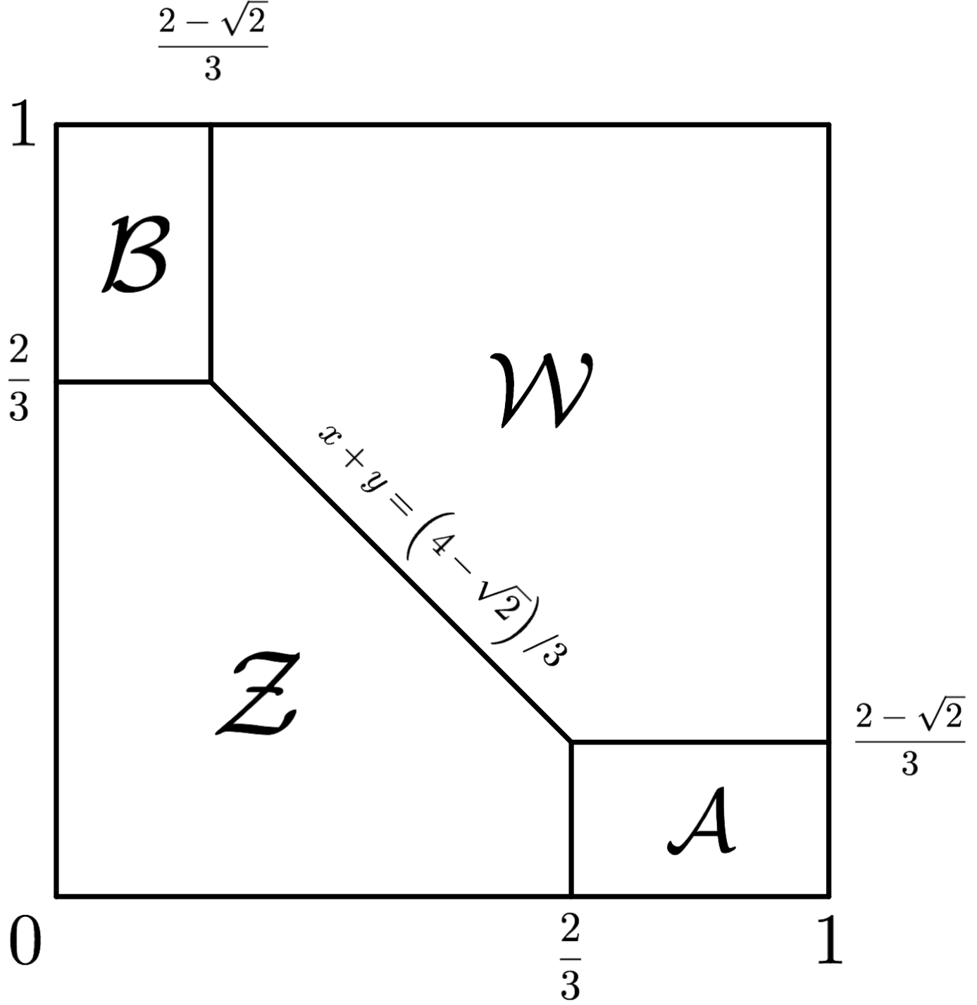
Example 1.

Let $n=2$, $m=1$ and $\rho$ be the Lebesgue measure on $X=[0,1]^{2}$. The square is divided in four parts as shown on FigureΒ 1 (the picture is taken from [14]). If the type of the bidder belongs to $\mathcal{Z}$, then the bidder receives no goods and pays nothing. In the region $\mathcal{A}$ the bidder receives the first good and pays $2/3$, in $\mathcal{B}$ the bidder receives the second good and pays $2/3$. Finally, in the region $\mathcal{W}$ the bidder receives both goods and pays $(4-\sqrt{2})/3$.

This examples demonstrates, in particular, that even in apparently simple cases the solution can not be reduced to one dimensional ones (the optimal mechanism neither sells goods together nor separately). See in this respect [14], D.2.

Refer to caption
Figure 1: Partition of the square for $n=2,m=1$ and the Lebesgue measure

Some other examples of explicit solutions can be found in [9].

2.4 The monopolist’s problem and Rochet representation

In the important particular case of $m=1$ bidder the auctioneer’s problem can be reduced to a maximization problem for functions (not to mechanisms). The problem turns out to be a particular case of the so-called monopolist’s problem. This approach goes back to Rochet (see [21] and the references therein). See also new results about the monopolist problem in [10], [17], [18], [3].

Let $m=1$. Given a mechanism $(P,T)$ let us consider the utility function

$$u(x)=\langle P(x),x\rangle-T(x)$$

(note that $(P,T)=(\overline{P},\overline{T})$).

Clearly, individually-rationality assumption is equivalent to $u\geq 0$. The incentive compatibility can be rewritten as follows:

$$u(x)=\langle P(x),x\rangle-T(x)\geq\langle P(x^{\prime}),x\rangle-T(x^{\prime})=u(x^{\prime})+\langle P(x^{\prime}),x-x^{\prime}\rangle.$$

Then it can be easily concluded that incentive compatibility is equivalent to convexity of $u$ and, in addition, one has:

$$P=\nabla u$$

(more precisely, $P\in\partial u$, where $\partial u$ is the subdifferential of $u$).

Thus the incentive compatible and individually-rational mechanism can be recovered from utility $u$. Clearly, feasibility $P_{i}\leq 1$ and nonnegativity $P_{i}\geq 0$ is equivalent to condition:

$$0\leq u_{x_{i}}\leq 1$$

for all $i$. We say that a function $f$ on $X$ is increasing, if $x_{i}\to f(x)$ is an increasing function for all fixed values xj,jβ‰ isubscriptπ‘₯𝑗𝑗𝑖x_{j},j\neq i. Clearly, for a differentiable function $f$ this is equivalent to assumption $f_{x_{i}}\geq 0$ for all $i$.

In what follows we denote by $\mathcal{U}$ the set of convex increasing functions satisfying $u(0)=0$.

Thus we get the following:

Theorem 1.

(Rochet) For $m=1$ bidder the auctioneer’s problem is equivalent to the problem of maximization of

$$\int_{[0,1]^{n}}\bigl{(}\langle x,\nabla u(x)\rangle-u(x)\bigr{)}\rho(x)dx$$

over all convex nonnegative functions $u$ on $[0,1]^{n}$ satisfying $0\leq u_{x_{i}}\leq 1$ for all $i$.

Equivalently maximization can be taken over functions belonging to $\mathcal{U}$.

Let us briefly describe another related problem: the so-called monopolist’s problem, going back to Mussa–Rosen [19]. Similarly to the auctioneer’s problem the initial formulation was given in terms of mechanisms and a reduction to optimization problem in certain class of utility functions has been obtained in a seminal paper of Rochet and ChonΓ© [21].

Monopolist’s problem: Given a function $\varphi$ and a probability distribution $\rho$ find maximum of

$$\Phi(u)=\int_{[0,1]^{n}}\bigl{(}\langle x,\nabla u(x)\rangle-u(x)-\varphi(\nabla u)\bigr{)}\rho(x)dx$$

on the set of convex increasing nonegative functions.

Function $\varphi$ is usually supposed to be convex and is interpreted as a cost of the (multidimensional) product $\nabla u$. In particular, choosing $\varphi=\delta_{[0,1]^{n}}$, we get the auctioneer’s problem for one bidder. Here indicator function $\delta_{A}$ is defined for a given set $A$ as follows : $\delta_{A}(x)=0$ for $x\in A$ and $\delta_{A}(x)=+\infty$ for $x\notin A$.

A systematic investigation of solutions to the monopolist’s problem was made in the seminal paper [21]. We emphasize that despite of a classical form of the "energy" functional $\Phi$, the convexity and monotonicity constraints makes unable the classical variational approach to the analysis of the monopolist problem. In general, any solution $u$ to this problem splits $X$ into three different regions:

  • β€’

    Indifference region

    $$\Omega_{0}=\{u=0\}$$
  • β€’

    Bunching region $\Omega_{1}$: uβ‰ 0𝑒0u\neq 0, $D^{2}u$ is degenerated

  • β€’

    Ξ©2subscriptΞ©2\Omega_{2}: $u$ is strictly convex: $D^{2}u>0$ (nonbunching regions).

The word "bunching" refers to a situation where a group of agents having different types are treated identically in the optimal solution. The standard technique of calculus of variation is available only inside of $\Omega_{1}$, where we get that $u$ solves the quasi-linear equation

$${\rm div}(\nabla\varphi(\nabla u))-1-{\rm div}(x\cdot\rho)=0.$$

Rochet and ChonΓ© suggested a hypothesis about explicit solution for $\varphi(x)=\frac{1}{2}|x|^{2}$ and $n=2$. However, their guess turns out to be wrong. Recently McCann and Zhang [18] gave a description of the solution partially based on rigorous proofs and partially on numerical simulations. An additional important ingredient is the proofs is a regularity result for solutions to monopolist’s problem obtained in [7]. As we will see, despite of the fact that the solution can be described in many details, it looks impossible to give a closed-form solution even in this model case.

More, precisely, McCann and Zhang studied the maximization problem

$$\int_{[a,a+1]^{2}}\biggl{(}\langle x,\nabla v(x)\rangle-v(x)-\frac{1}{2}|\nabla v(x)|^{2}\biggr{)}\,dx\to\max,\quad v\in\mathcal{U}.$$ (9)

They proved that the solution $v$ splits $[a,a+1]^{2}$ into the following regions:

$\displaystyle\{\nabla v=0\}$ $\displaystyle\subset$ $\displaystyle\Omega_{0}=\{(x,y)\in[a,a+1]^{2}\colon x+y<a+y_{0}\},$
$\displaystyle\{\det D^{2}v=0,\ \nabla v>0\}$ $\displaystyle\subset$ $\displaystyle\Omega_{1}=\Omega^{0}_{1}\cup\Omega^{\pm}_{1},$ (10)
$\displaystyle\{\det D^{2}v>0\}$ $\displaystyle\subset$ $\displaystyle\Omega_{2}=\mathop{\mathrm{cl}}([a,a+1]^{2}\backslash(\Omega_{0}\cup\Omega_{1})),$

where

$\displaystyle\Omega^{0}_{1}$ $\displaystyle=$ $\displaystyle\{(x,y)\in[a,a+1]^{2}\colon a+y_{0}\leq x+y\leq a+y_{1}\},$
$\displaystyle\Omega^{\pm}_{1}$ $\displaystyle=$ $\displaystyle\{(x,y)\in\Omega_{1}\backslash\Omega^{0}_{1}\colon\pm(x-y)\geq 0\}.$

According to [7] every solution $v$ to (9) belongs to $C^{1}$. This information was used to construct the solution $v$ as follows:

  1. 1.
    $$v(x,y)=0,\quad(x,y)\in\Omega_{0}.$$ (11)
  2. 2.
    $$v(x,y)=\frac{3}{8}(x+y)^{2}-\frac{a}{2}(x+y)-\frac{1}{2}\ln(x+y-2a)+C_{0},\quad(x,y)\in\Omega^{0}_{1},$$ (12)

    for some $C_{0}$, defined by property of regularity of $v$ on $\partial\Omega^{0}_{1}\cap\partial\Omega^{\pm}_{1}$

  3. 3.

    Function $v$ has the following form on $\Omega^{-}_{1}$:

    $$v(x,y)=v(z(r,\theta))=m(\theta)r+b(\theta),\quad(x,y)\in\Omega^{-}_{1},$$ (13)

    where

    $$z(r,\theta)=(a,h(\theta))+r(\cos\theta,\sin\theta),\quad\theta\in\Bigl{(}-\frac{\pi}{4},\frac{\pi}{2}\Bigr{]},r\in[0,R(\theta)],$$

    for some functions $R\colon[-\frac{\pi}{4},\frac{\pi}{2}]\to[0,\sqrt{2})$ and $m,b$. Function $v$ is symmetrically extended to $\Omega^{\pm}_{1}$.

  4. 4.
    $$\begin{cases}\Delta v_{2}(x,y)=3,&(x,y)\in\mathop{\mathrm{Int}}\Omega_{2};\\ \langle\nabla v_{2}(x,y),n(x,y)\rangle=\langle(x,y),n(x,y)\rangle,&(x,y)\in\partial\Omega_{2}\cap\partial X;\\ v_{2}=\left.v\right|_{\Omega_{1}},&(x,y)\in\partial\Omega_{1}\cap\partial\Omega_{2}.\end{cases}$$ (14)
  5. 5.

    In addition, since $v\in C^{1}(X)$, one has to assume the Neumann boundary condition

    $$\langle\nabla v_{2}(x,y),n(x,y)\rangle=\langle\nabla v_{1}(x,y),n(x,y)\rangle,\quad(x,y)\in\partial\Omega_{1}\cap\partial\Omega_{2},$$ (15)

    here $v_{1}:=\left.v\right|_{\Omega_{1}}$.

The main result of [18] is the following characterization.

Theorem 2.

Assume that $v\in\mathcal{U}$ satisfies (11) – (15), and $v$, $\Omega_{2}$ are Lipschitz. Then $v$ is the unique solution toΒ (9).

2.5 Stochastic domination and reduction to maximization problem for functions

Does there exist a reduction in the spirit of Theorem 1 for many bidders? The answer is affirmative and the approach heavily relies on the symmetry of mechanism. Let us start with the result of Hart and Reny [13] for the case of $n=1$ item. Some earlier results in this spirit were obtained by Matthews [16] and Border [5].

It turns out that the marginals of a feasible mechanism can be characterized in terms if stochastic dominance.

Let for simplicity $n=1$. First, without loss of generality we can restrict ourselves to symmetric mechanisms. If $(P,T)$ is not symmetric, we can symmetrize it :

(Pjs​y​m​(x1,β‹―,xm),Tjs​y​m​(x1,β‹―,xm))=1m!β€‹βˆ‘Οƒ(Pσ​(j)​(xσ​(1),β‹―,xσ​(m)),Tσ​(j)​(xσ​(1),β‹―,xσ​(m))),superscriptsubscriptπ‘ƒπ‘—π‘ π‘¦π‘šsubscriptπ‘₯1β‹―subscriptπ‘₯π‘šsuperscriptsubscriptπ‘‡π‘—π‘ π‘¦π‘šsubscriptπ‘₯1β‹―subscriptπ‘₯π‘š1π‘šsubscript𝜎subscriptπ‘ƒπœŽπ‘—subscriptπ‘₯𝜎1β‹―subscriptπ‘₯πœŽπ‘šsubscriptπ‘‡πœŽπ‘—subscriptπ‘₯𝜎1β‹―subscriptπ‘₯πœŽπ‘š\bigl{(}P_{j}^{sym}(x_{1},\cdots,x_{m}),T_{j}^{sym}(x_{1},\cdots,x_{m})\bigr{)}=\frac{1}{m!}\sum_{\sigma}\bigl{(}P_{\sigma(j)}(x_{\sigma(1)},\cdots,x_{\sigma(m)}),T_{\sigma(j)}(x_{\sigma(1)},\cdots,x_{\sigma(m)})\bigr{)},

where the sum is taken over all the permutations of the bidders.

Clearly, the symmetrized mechanism satisfies the same restrictions and gives the same value to the revenue. At this step we use that all the bidders are independently and identically distributed. Thus without loss of generality everywhere below we will talk about symmetric mechanisms.

Consider $\overline{P}$ defined by (5) and for a fixed $\alpha\in\mathbb{R}_{+}$ set $A=\{x:\overline{P}(x)>\alpha\}\subset X.$ Using symmetry and feasibility of the mechanism one obtains:

$\displaystyle m\int_{X}\overline{P}(x)I_{A}(x)\rho dx$ $\displaystyle=\int_{\overline{X}}\Bigl{(}\sum_{j=1}^{m}P_{j}(x_{j})I_{A}(x_{j})\Bigr{)}\overline{\rho}dx$
$\displaystyle\leq\int_{\overline{X}}I_{\exists j:x_{j}\in A}(x_{1},\cdots,x_{m})\overline{\rho}dx=1-\Bigl{(}\int_{A^{c}}\rho(x)dx\Bigr{)}^{m}.$

Put $p=\int_{A^{c}}\rho dx$.

$\displaystyle\int_{X}$ $\displaystyle\bigl{(}\overline{P}-\alpha\bigr{)}_{+}\rho dx=\int_{A}\overline{P}dx-\alpha(1-p)\leq\frac{1}{m}-\frac{p^{m}}{m}-\alpha(1-p)$
$\displaystyle\leq\frac{1}{m}-\alpha+\frac{m-1}{m}\alpha^{\frac{m}{m-1}}=\int_{0}^{1}(t^{m-1}-\alpha)_{+}dt.$

Since the convex hull of functions $(x-\alpha)_{+}$ are precisely convex increasing functions, we obtain the following important property:

$$\int_{0}^{1}f(\overline{P})\rho dx\leq\int_{0}^{1}f(t^{m-1})dx$$

for every convex increasing function $f$, i.e. the distribution of $\overline{P}$ is stochastically dominated by the distribution of $\xi^{m-1}$, where $\xi$ is uniformly distributed on $[0,1]$. In what follows we write:

$$\overline{P}\preceq\xi^{m-1}$$

It was shown by Hart and Reny that the converse is also true: of $\nu\preceq\xi^{m-1}$, then $\nu$ is a distribution of $\overline{P}$ for some symmetric mechanism $P$.

The general result for many bidders and items unifying results of Rochet and Hart–Reny was obtained in [14]. In the same way as for $n=1$ we define for a feasible symmetric mechanism $(P,T)$, satisfying (8) and (7):

$$u(x)=\langle\overline{P}_{1}(x),x\rangle-\overline{T}_{1}(x).$$

Then we prove that $u$ is convex, nonnegative and increasing ((7), (8)), see [14], Lemma 2. Moreover we conclude that

$$\overline{P}_{1}=\nabla u(x)$$

and, repeating the above arguments, we prove that the distribution of $\overline{P}_{1,i}$ is stochastically dominated by the distribution of $\xi^{m-1}$. Conversely, using the Hart–Reny theorem we can show that every $u\in\mathcal{U}$ satisfying $u_{x_{i}}\preceq\xi^{m-1}$ defines feasible, individually rational, incentive compatible mechanism on $X^{m}$ with the same total revenue ([14], Lemma 3). Thus we get the following:

Theorem 3.

The value of the general auctioneer’s problem coincides with the maximum of

$$m\int_{[0,1]^{n}}\bigl{(}\langle x,\nabla u(x)\rangle-u(x)\bigr{)}\rho(x)dx$$

over all convex nonnegative increasing functions $u$ on $[0,1]^{n}$ satisfying $u_{x_{i}}\preceq\xi^{m-1}$, where $\xi$ is uniformly distributed on $[0,1]$ for all $i$.

Remark 1.

It is easy to check that without loss of generality one can assume that $u(0)=0$. Thus the functional in the auctioneer’s problem can be equivalently rewritten in the form

$$m\int_{[0,1]^{n}}\bigl{(}\langle x,\nabla u(x)\rangle-u(x)\bigr{)}\rho(x)dx+mu(0).$$

3 Mass transportation problem

In this section we briefly recall some facts about optimal transportation theory, which are important for application to the auction design. A comprehensive presentation of the mathematical theory of transportation can be found in the books byΒ [22] and [23] and in survey [4].

3.1 General optimal transportation problem

Let $\mu$ and $\nu$ be probability measures on measurable spaces $X$ and $Y$, and let $c:X\times Y\to\mathbb{R}$ be a measurable function. The classical Kantorovich problem is the minimization problem

$$\int_{X\times Y}c(x,y)\leavevmode\nobreak\ d\pi\to\inf$$

on the space Π​(ΞΌ,Ξ½)Ξ πœ‡πœˆ\Pi(\mu,\nu) of probability measures on $X\times Y$ with fixed marginals $\pi_{x}=\mu$ and $\pi_{y}=\nu$.

It is well-known that this problem is closely related to another linear programming problem, which is called β€˜β€˜dual transportation problem’’

$$\int f\leavevmode\nobreak\ d\mu+\int g\leavevmode\nobreak\ d\nu\to\sup.$$

The dual transportation problem is considered on the couples of integrable functions $(f,g)$, satisfying $f(x)+g(y)\leq c(x,y)$ for all $x\in X$, $y\in Y$.

These problems are linear programming problems and under broad assumptions the values of both problems coincide. Complementary slackness condition gives that

$$f(x)+g(y)=c(x,y)$$

for $\pi$-almost all $(x,y)$.

3.2 $L^{1}$-transportation problem

The case when $X=Y=\mathbb{R}^{N}$ and $c(x,y)=|x-y|$, where $|\cdot|$ is a norm, is special. In this case the solution $(f,g)$ to the dual problem satisfies $f=-g$ and, in addition, $f$ is a $1$-Lipschitz function with respect to $|\cdot|$: $|f(x)-f(y)|\leq|x-y|$. Thus the value of the dual problem equals

$$W_{1}(\mu-\nu)=\max\left\{\int\limits_{X}ud(\mu-\nu):u\in Lip(X)\right\}.$$

The functional $W_{1}$ is a norm on the space of the signed finite measures.

The transport density $\sigma$ is a measure related to the solution $\gamma$ as follows:

$$\sigma(B)=\int\limits_{X\times Y}\mathcal{H}^{1}([x,y]\cap B)\gamma(dx\,dy),$$

where $\mathcal{H}^{1}$ is the one-dimensional Hausdorff measure, $[x,y]$ is the segment joining $x$ and $y$. The transport density satisfies the following equation

$$\mu-\nu=-{\rm div}(\nabla u\cdot\sigma),$$

which is understood in the weak sense.

More generally, given a cost $c(x,y)$ and a signed measure $\pi$ on $X=Y$ satisfying $\pi(X)=0$, one can consider optimal transshipment problem

$$\int_{X\times Y}c(x,y)d\gamma\to\min,$$

where $\gamma$ satisfies $\gamma_{x}-\gamma_{y}=\pi$. The dual problem takes the form

$$\int_{X}ud\pi\to\max$$

over functions satisfying $u(x)-u(y)\leq c(x,y)$.

3.3 Beckmann’s problem.

Beckmann’s problem was introduced in [2] to model commodity flows. Mathematically it can be stated as follows: we are given a (convex) function $\varphi$ and a measure $\pi$ on $\mathbb{R}^{N}$ with $\pi(\mathbb{R}^{N})=0$. Then

$${\rm Beck}_{\varphi,\rho}(\pi)=\inf\left\{\int_{\mathbb{R}^{N}}\varphi(c(x))\rho dx,\quad-\operatorname{div}(c\cdot\rho)=\pi\right\},$$

where $c$ is a vector field and divergence is understood in the weak sense

$$\int_{\mathbb{R}^{N}}\left\langle\nabla f,c\right\rangle dx=\int_{\mathbb{R}^{N}}fd\pi,$$

for all sufficiently smooth $f$.

If $\varphi$ is a norm on $\mathbb{R}^{n}$, the Beckmann problem is equivalent to the $L^{1}$-transportation problem (see [22]).

3.4 Congested transport

Beckmann’s problem is equivalent to a Monge-Kantorovich-type problem called β€˜β€˜congested optimal transport’’; see [22] for the detailed presentation and references. Let us describe the equivalence informally for Beckmann’s problem with the weight $\rho\equiv 1$. Given a domain $\Omega$ of a Euclidean space, an absolutely continuous supply-demand imbalance measure $\pi$ on $\Omega$ satisfying $\pi(\Omega)=0$, and a convex function $\Phi$, the following identity holds:

$$\inf_{c:\,{\mathrm{div}}[c]+\pi=0}\int\Phi(c){\,\mathrm{d}}x=\inf_{Q:\,Q_{1}-Q_{0}+\pi=0}\int_{\Omega}\Phi(i_{Q}){\,\mathrm{d}}x.$$ (16)

Here $Q$ ranges over to the set of all probability measures on β€˜β€˜curves’’, i.e., continuous mappings $\gamma\colon[0,1]\to\Omega$, and $Q_{t}$ denotes the probability measure on $\Omega$ obtained as the image of $Q$ under the map $\gamma\to\gamma(t)\in\Omega$. The object $i_{Q}$ is the so-called traffic intensity function which is defined so that the following identity holds for any test function $\varphi$:

$$\int_{\Omega}\varphi(x)i_{Q}(x){\,\mathrm{d}}x=\int\left(\int_{0}^{1}\varphi(\gamma(t))|\gamma^{\prime}(t)|{\,\mathrm{d}}t\right){\,\mathrm{d}}Q(\gamma)$$

Formula (16) can be seen as a Lagrangian formulation of Beckmann’s problem taking a form of a β€˜β€˜problem for measures on curves.’’ It is a quasi-dynamical formulation, a version of which is well known for the Monge-Kantorovich transportation problem; see [23].

3.5 Weak transport

Let $\mu,\nu$ be probability measures on $X$. Assume we are given a cost function

$$c:X\times\mathcal{P}(X)\to\mathbb{R}_{+},$$

where $\mathcal{P}(X)$ is the space of probability measures on $X$. Consider the following nonlinear optimization problem

Kc​(Ξ½|ΞΌ):=infΟƒβˆˆΞ β€‹(ΞΌ,Ξ½)∫Xc​(x,Οƒx)​μ​(d​x),assignsubscript𝐾𝑐conditionalπœˆπœ‡subscriptinfimumπœŽΞ πœ‡πœˆsubscript𝑋𝑐π‘₯superscript𝜎π‘₯πœ‡π‘‘π‘₯K_{c}(\nu|\mu):=\inf_{\sigma\in\Pi(\mu,\nu)}\int_{X}c(x,\sigma^{x})\mu(dx), (17)

where $\sigma^{x}$ are conditional distributions, i.e. identity

$$\int_{X\times X}f(x,y)\sigma(dx\,dy)=\int_{X}\int_{X}f(x,y)\sigma^{x}(dy)\mu(dx)$$

holds for every bounded Borel $f$. This problem is called weak (nonlinear) mass transportation problem.

An important particular case of this problem is given by $c(x,y)=|x-\int yp_{x}(dy)|$, where $|\cdot|$ is a norm. Then the dual problem takes the form

$$\sup\left\{\int_{X}\varphi d\mu-\int_{X}\varphi d\nu\right\},$$

where the supremum is taken over all convex $1$-Lipschitz functions (see [12]).

This problem attracts a lot of attention withing the last decade. We refer to the nice survey paper [1], where refer can find a long list of applications (measure concentration, SchrΓΆdinger problem, martingale optimal transport).

Let us mention, in particular, a nice proof by duality of the Strassen theorem about characterization of the marginals of martingales (see [12]). Apart from auctions, some applications of weak transport in economics (labor theory) were found in [8].

4 Mass transportation in $1$-bidder case

A remarkable relation of the $1$-bidder problem to the mass transportation problem was discovered by Daskalakis, Deckelbaum and Tzamos in [9]. The main idea of [9] was to rewrite the auctioneer’s functional using integration by parts. Indeed, assume that $\rho$ is sufficiently regular (at least $C^{1}(X)$). Then

$\displaystyle m\int_{[0,1]^{n}}\bigl{(}\langle x,\nabla u(x)\rangle-u(x)\bigr{)}\rho(x)dx+mu(0)=$
$\displaystyle m\Big{(}\int_{\partial[0,1]^{n}}u\langle x,\nu\rangle\rho d\mathcal{H}^{n-1}-\int_{[0,1]^{n}}\bigl{(}\langle x,\nabla\rho(x)\rangle+(n+1)\rho(x)\bigr{)}udx+u(0)\Bigr{)}.$

Here $\mathcal{H}^{n-1}$ is the Hausdorff measure of dimension $n-1$ and $\nu$ is the outer normal to $\partial X$. We rewrite the auctioneer’s problem in the form

$$\int_{X}ud\mu\to\max,$$

where $u$ is convex and increasing and

$$\mu=m\Bigl{(}\langle x,\nu\rangle\rho\mathcal{H}^{n-1}-(n+1)\rho dx-\langle x,\nabla\rho(x)\rangle dx+\delta_{0}\Bigr{)}$$

is a signed measure with zero balance: $\mu(X)=0$. We will call $\mu$ transform measure.

Finally, we get the following reformulation of the auctioneer’s problem with $1$ bidder: find

$$\max_{u\in\mathcal{U},u\in{\rm Lip}_{1}(X)}\int ud\mu$$

on the set of convex increasing $1$-Lipschitz functions.

In this form the problem looks quite similar to the dual transportation problem, especially to the dual weak $L^{1}$-transportation problem. Indeed, additional constraints on $u$ lead naturally to a variant of the weak transportation problem.

Theorem 4.

(Daskalakis–Deckelbaum–Tzamos). The $1$-bidder problem is equivalent to a weak transportation problem. In particular, the following duality relation holds:

$$\max_{u\in\mathcal{U},u\in{\rm Lip}_{1}(X)}\int ud\mu=\min_{\gamma\in\Gamma}\int_{X^{2}}\|x-y\|_{1}\gamma(dxdy),$$

where $\Gamma$ is the set of nonnegative measures on $X^{2}$ satisfying $Pr_{1}\gamma\succeq\mu_{+}$, $Pr_{2}\gamma=\mu_{-}$.

Remark 2.

Moreover, another duality relation holds for the related weak transshipment problem:

$$\max_{u\in\mathcal{U},u\in{\rm Lip}_{1}(X)}\int ud\mu=\min_{\gamma:\pi\succeq\mu}\int_{X^{2}}\|x-y\|_{1}\gamma(dxdy),$$

where $\pi=Pr_{1}\gamma-Pr_{2}\gamma$.

The proof of Theorem 4 is based on the application of the so-called Fenchel–Rockafellar duality. Given two convex functionals $\Theta,\Xi$ with values in $\mathbb{R}\cup\{+\infty\}$ on a normed space $E$ one has the following form of the minimax principle:

$$\inf_{z\in E}\bigl{(}\Theta(z)+\Xi(z)\bigr{)}=\max_{z^{*}\in E^{*}}\bigl{(}-\Theta(-z^{*})-\Xi(z^{*})\bigr{)},$$ (18)

provided there exists a point $z_{0}$ such that $\Theta(z_{0})<\infty,\Xi(z_{0})<\infty$, and $\Theta$ is continuous at $z_{0}$. The latter conditions is needed for application of the Hahn-Banach separation theorem and establishing the existence of the maximum point at the right-hand side of the duality. The proof can be found in [23].

The direct application of the Fenchel–Rockafellar duality to the functionals

$$\Theta(f)=\begin{cases}0,&\mbox{if}\ f(x,y)\geq-\|x-y\|_{1}\\ +\infty,&\mbox{in the opposite case}\end{cases}$$
$$\Xi(f)=\begin{cases}\int\psi d\mu_{-}-\int\phi d\mu_{+},&\mbox{if}f(x,y)=\psi(y)-\phi(x),\mbox{where}\ \psi,\phi\in\mathcal{U}(X)\\ +\infty,&\mbox{in the opposite case.}\end{cases}$$

gives

$$\min_{Pr_{1}\gamma\succeq\mu_{+},Pr_{2}\gamma\preceq\mu_{-}}\int_{X^{2}}\|x-y\|_{1}\gamma(dxdy)=\sup_{\phi,\psi\in\mathcal{U},\phi(x)-\psi(y)\leq\|x-y\|_{1}}\Bigl{(}\int\phi d\mu_{+}-\int\psi d\mu_{-}\Bigr{)},$$

where $\gamma$ is a measure on $X^{2}$ with

$$\gamma_{+}(X)=\gamma_{-}(X)=\mu_{+}(X)=\mu_{-}(X).$$

The proof will be completed if we show that without loss of generality one can assume $\varphi=\psi$ and replace condition $Pr_{1}\gamma\succeq\mu_{+}$ with $Pr_{1}\gamma=\mu_{+}$.

The first statement was proved in [9], Lemma 5. Given $\phi\in\mathcal{U}$ define $\overline{\psi}(y)=\sup_{x}(\varphi(x)-\|x-y\|_{1})$. It is clear that

$$\int\phi d\mu_{+}-\int\psi d\mu_{-}\leq\int\phi d\mu_{+}-\int\overline{\psi}d\mu_{-}.$$

Then one can show that $\overline{\psi}\in\mathcal{U}$ and, moreover, $\overline{\psi}=\phi$. Thus the replacement of $(\phi,\psi)$ with $(\phi,\overline{\psi})=(\phi,\phi)$ will increase the value of the functional.

The second statement was proved in [1] Theorem 6.1. by the following argument: given $\gamma$ with $Pr_{1}\gamma\succeq\mu_{+},Pr_{2}\gamma\preceq\mu_{-}$ let $\xi,\eta$ be $X$-valued random variables satisfying

$$\xi_{1}\sim\mu_{+},\\ \eta_{2}\sim\mu_{-},\\ (\xi_{2},\eta_{1})\sim\gamma.$$

and

$$\xi_{1}\leq\mathbb{E}(\xi_{2}|\xi_{1}),\ \eta_{1}\leq\mathbb{E}(\eta_{2}|\eta_{1}).$$

Such variables can be easily built with the help of Strassen theorem. We will prove the statement if we show that there exists a variable $Z$ satisfying $Z\preceq\mu_{-}$ and $\mathbb{E}\|\xi_{2}-\eta_{1}\|_{1}\geq\mathbb{E}\|\xi_{1}-Z\|_{1}.$ Define

$$Z=\xi_{1}+\mathbb{E}(\eta_{1}-\xi_{2}|\xi_{1}).$$

Indeed,

$\displaystyle Z\preceq Z+\mathbb{E}(\xi_{2}-\xi_{1}|\xi_{1})=\mathbb{E}(\eta_{1}|\xi_{1})\preceq\eta_{1}\preceq\eta_{2}\sim\mu_{-}.$

Finally, by Jenssen’s inequality

$$\mathbb{E}\|\xi_{2}-\eta_{1}\|_{1}\geq\mathbb{E}\|\mathbb{E}(\xi_{2}-\eta_{1}|\xi_{1})\|_{1}=\mathbb{E}\|\xi_{1}-Z\|_{1}.$$

Let us revisit Example 1. The solution $u$ and the majorizing measure $\pi$ are given below (see the details in [9]).

The optimal function $u=u^{\mathrm{opt}}$ is given by

$$u^{\mathrm{opt}}(x,y)=\begin{cases}0&(x,y)\in\mathcal{Z}\\ x-\frac{2}{3}&(x,y)\in\mathcal{A}\\ y-\frac{2}{3}&(x,y)\in\mathcal{B}\\ x+y-\frac{4-\sqrt{2}}{3}&(x,y)\in\mathcal{W}.\end{cases}$$ (19)

The answers for the transform measure $\mu$ and for the optimal β€˜β€˜imbalance’’ $\pi=\pi^{\mathrm{opt}}$ majorizing $m$ are as follows:

$$\mu=\delta_{0}+\lambda_{1}|_{[0,1]\times\{0\}}+\lambda_{1}|_{\{0\}\times[0,1]}-3\lambda_{2}|_{[0,1]^{2}},$$ (20)
$$\pi^{\mathrm{opt}}=\lambda_{1}|_{[0,1]\times\{0\}}+\lambda_{1}|_{\{0\}\times[0,1]}-3\lambda_{2}|_{[0,1]^{2}\setminus\mathcal{Z}},$$ (21)

where $\lambda_{2},\lambda_{1}$ are the two- and one-dimensional Lebesgue measures, respectively.

5 Duality for $n$-bidder case

In this section we prove a duality statement for the $n$-bidder case. The results were obtained in [14]. We show, in particular, that the dual problem us naturally related to the Beckmann’s transportation problem.

5.1 Duality in the monopolist’s problem

An important auxiliary result is the duality theorem in monopolist’s problem. Informally, the duality relation looks as follows: given a convex function $\varphi$ and a measure $\mu$ of finite variation satisfying $\mu(X)=0$ one has:

$$\sup_{u\in\mathcal{U}}\Bigl{(}\int_{X}ud\mu-\int_{X}\varphi(\nabla u)\rho dx\Bigr{)}=\inf_{c:-{\rm div}(c\cdot\rho)\succeq\mu}\int_{X}\varphi^{*}(c)\rho dx.$$

Here $\mathcal{U}$ is the set of convex increasing functions on $X$ and divergence is a signed measure ${\rm div}(c\cdot\rho)$. We always understand it in the weak (integration by parts) sense: for a smooth function $\psi$ on $X$ one has

$$\int_{X}\psi d{\rm div}(c\cdot\rho)=-\int_{X}\langle\nabla\psi,c\rangle\rho dx.$$

As usual, inequality $\sup\leq\inf$ is easy to verify:

$$\int_{X}ud\mu-\int_{X}\varphi(\nabla u)\rho dx\leq-\int_{X}ud{\rm div}(c\cdot\rho)-\int_{X}\varphi(\nabla u)\rho dx=\int_{X}\langle\nabla u,c\rangle\rho dx-\int_{X}\varphi(\nabla u)\rho dx\leq\int_{X}\varphi^{*}(c)\rho dx.$$

By complementary slackness argument we conclude that in the absence of the duality gap the extremizers $u_{0},c_{0}$ must satisfy

$$c_{0}\in\partial\varphi(\nabla u_{0}).$$

The rigorous proofs of different versions of this result can be found

1. In [14] Proposition 6,7. The proof relies on a version of minimax theorem (Sion’s theorem) using compactness of one of the spaces. This leads to essential restrictions on $\varphi$.

2. In [18]. Function $\varphi$ is assumed to be strictly convex. In the McCann–Zhang formulation the assumption $-{\rm\mathrm{div}}(c\cdot\rho)\succeq\mu$ is replaced by another assumption, which does not presume any regularity of the vector field $c$:

$$\int_{X}ud\mu\leq\int_{X}\langle c,\nabla u\rangle\rho dx,$$

for all $u\in\mathcal{U}$ (see also Section 4 below). The proof is based on the Fenchel–Rockafellar duality and some regularization of the problem.

3. Another relatively simple and general proof based on the use of the Fenchel–Rockafellar duality as well was given in [3].

To understand informally the duality statement let us observe the following simple duality relation: given a convex function $\varphi$ and a distribution $\rho$ let us define the energy functional:

$$\Theta(u)=\begin{cases}\int_{X}\varphi(\nabla u)\rho dx,\ u\in W^{1,1}(X),\\ +\infty,&\mbox{in the opposite case}.\end{cases}$$ (22)

Here the standard notation $W^{1,1}(X)$ is used for the classical Sobolev space.

Theorem 5.

The Legendre transform

$$\Theta^{*}(\mu)=\sup_{u}\Bigl{(}\int ud\mu-\Theta(u)\Bigr{)}.$$

of the energy functional (22) coincides with the Beckmann transportation functional (23) for the dual potential $\varphi^{*}$.

Ξ˜βˆ—β€‹(ΞΌ)={+∞,if​μ​(X)β‰ 0,infc:div​(ρ⋅c)=βˆ’ΞΌβˆ«XΟ†βˆ—β€‹(c)​ρ​𝑑x,if​μ​(X)=0.superscriptΞ˜πœ‡casesifπœ‡π‘‹0subscriptinfimum:𝑐divβ‹…πœŒπ‘πœ‡subscript𝑋superscriptπœ‘π‘πœŒdifferential-dπ‘₯ifπœ‡π‘‹0\Theta^{*}(\mu)=\begin{cases}+\infty,&\mbox{if}\ \mu(X)\neq 0,\\ \inf_{c:{\rm div}(\rho\cdot c)=-\mu}\int_{X}\varphi^{*}(c)\rho dx,&\mbox{if}\ \mu(X)=0.\end{cases} (23)

As usual, it is easy to see that one functional dominates another: indeed, for all admissible $(u,\mu,c)$ one has

$$\int ud\mu-\Theta(u)=-\int ud{\rm div}(\rho\cdot c)-\Theta(u)=\int\langle\nabla u,c\rangle\rho dx-\int\varphi(\nabla u)\rho dx\leq\int\varphi^{*}(c)\rho dx.$$

Hence

$$\inf_{c:{\rm div}(\rho\cdot c)=-\mu}\int_{X}\varphi^{*}(c)\rho dx\geq\sup_{u}\Bigl{(}\int ud\mu-\Theta(u)\Bigr{)}.$$

The proof of the equality $\inf=\sup$ can be found (in slightly different settings) in [6], [22], [3].

Theorem 6.

Let $\varphi$ be a convex lower semicontinuous function, finite on $X=[0,1]^{n}$ and taking $+\infty$-value outside of $X$. Let $\mu\in\mathcal{M}_{0}$, where $\mathcal{M}_{0}$ is the space of measures with finite variation satisfying $\mu(X)=0$. Then the following duality relation holds:

$$\max_{u\in\mathcal{U}(X)}\Phi(u)=\inf_{\pi\in\mathcal{M}_{0}:\mu\preceq\pi}{\rm Beck}_{\rho,\varphi^{*}}(\pi),$$

where

$$\Phi(u)=\biggl{(}\int_{X}ud\mu-\int_{X}\varphi(\nabla u)\rho dx\biggr{)},\ {\rm Beck}_{\rho,\varphi^{*}}(\pi)=\inf_{c\colon\pi+{\rm div}(c\cdot\rho)=0}\int_{X}\varphi^{*}(c)\rho dx.$$
Remark 3.

We warn the reader that it was mistakenly claimed in [3] that the infimum in the duality relation can be always reached on some measure $\pi$ of finite variation.

We give a proof of this result under assumption that $\varphi$ is bounded on $X$ and infinite on $\mathbb{R}^{n}\setminus X$.

Sketch of the proof of Theorem 6: We consider functionals $\Theta,\Xi$ on the space of continuous functions $E=C(X)$ equipped with the uniform norm and functionals $\Theta^{*},\Xi^{*}$ on the dual space $\mathcal{M}(X)$ of signed measures with finite variation. We denote by $E_{0}\subset E$ the subspace of functions satisfying $x(0)=0$ and by $\mathcal{M}_{0}(X)$ the subset of $\mathcal{M}(X)$ satisfying $\mu(X)=0$.

Let us consider functional

$$\Xi(u)=\begin{cases}-\int_{X}ud\mu,&u\in\mathcal{U}\\ +\infty,&\mbox{in the opposite case}\end{cases}$$

It is easy to check that $\Xi$ is convex and its Legendre transform satisfies

$\displaystyle\Xi^{*}(\nu)$ =supu∈E(∫Xu​𝑑μ+∫Xu​𝑑ν)={+∞,if​ν​(X)β‰ 0,supuβˆˆπ’°βˆ«Xu​d​(ΞΌ+Ξ½),if​ν​(X)=0,absentsubscriptsupremum𝑒𝐸subscript𝑋𝑒differential-dπœ‡subscript𝑋𝑒differential-d𝜈casesifπœˆπ‘‹0subscriptsupremum𝑒𝒰subscriptπ‘‹π‘’π‘‘πœ‡πœˆifπœˆπ‘‹0\displaystyle=\sup_{u\in E}\biggl{(}\int_{X}ud\mu+\int_{X}ud\nu\biggr{)}=\begin{cases}+\infty,&\mbox{if}\ \nu(X)\neq 0,\\ \sup_{u\in\mathcal{U}}\int_{X}ud(\mu+\nu),&\mbox{if}\ \nu(X)=0,\end{cases}

Note that

$$-\max_{u\in\mathcal{U}_{0}}\biggl{(}\int_{X}ud\mu-\int_{X}\varphi(\nabla u)\rho dx\biggr{)}=\min_{u\in E}\Bigl{(}\Theta(u)+\Xi(u)\Bigr{)}.$$

We apply the following duality to be proved later :

$$\inf_{u\in E}\Bigl{(}\Theta(u)+\Xi(u)\Bigr{)}=-\inf_{\nu\in\mathcal{M}(X)}\Bigl{(}\Theta^{*}(-\nu)+\Xi^{*}(\nu))\Bigr{)}.$$ (24)

One has

$\displaystyle\max_{u\in\mathcal{U}}$ $\displaystyle\biggl{(}\int_{X}ud\mu-\int_{X}\varphi(\nabla u)\rho dx\biggr{)}=\inf_{\nu\in\mathcal{M}(X)}\Bigl{(}\Theta^{*}(-\nu)+\Xi^{*}(\nu))\Bigr{)}$
$\displaystyle=\inf_{\nu\in\mathcal{M}_{0},\nu\preceq-\mu}\Theta^{*}(-\nu)=\inf_{\nu\in\mathcal{M}_{0},\mu\preceq\nu}\Theta^{*}(\nu)=\inf_{\nu\in\mathcal{M}_{0},\mu\preceq\nu}{\rm Beck}_{\rho,\varphi^{*}}(\nu).$

Let us prove (24). Note that (18) is different from (24), because (24) does not claim that mininum can be reached. We follow the proof of [23, Theorem 1.9]. Relation (24) is equivalent to the following:

$$\inf_{u\in E}\Bigl{(}\Theta(u)+\Xi(u)\Bigr{)}=\sup_{\nu\in E^{*}}\inf_{u,v\in E}\biggl{(}\Theta(u)+\Xi(v)+\int_{X}(u-v)d\nu\biggr{)}.$$

Taking $u=v$, one gets

$$\inf_{u\in E}\Bigl{(}\Theta(u)+\Xi(u)\Bigr{)}\geq\sup_{\nu\in E^{*}}\inf_{u,v\in E}\biggl{(}\Theta(u)+\Xi(v)+\int_{X}(u-v)d\nu\biggr{)}.$$

It is sufficient to prove that there exists a sequence $\nu_{n}\in\mathcal{M}$ such that

$$\Theta(u)+\Xi(v)+\int_{X}(u-v)d\nu_{n}+\frac{1}{n}\geq\inf_{u\in E}\Bigl{(}\Theta(u)+\Xi(u)\Bigr{)}\quad\forall\,u,v\in E.$$

Since $\Theta,\Xi$ a both invariant with respect to addition of a constant, the desired inequality is possible if and only if $\nu_{n}\in\mathcal{M}_{0}$. Thus from the very beginning we take $u,v\in E_{0}$. Note that any functional frΠΎm $E^{*}_{0}$ can be identified with $\mathcal{M}_{0}$.

Thus the problem is reduced to the following: prove existence of $\nu_{n}\in\mathcal{M}_{0}$ such that

$$\Theta(u)+\Xi(v)+\int_{X}(u-v)d\nu_{n}+\frac{1}{n}\geq\inf_{u\in E_{0}}\Bigl{(}\Theta(u)+\Xi(u)\Bigr{)}\ \ \forall\,u,v\in E_{0}.$$

Let us define

Cn={(u,t)∈E0×ℝ;maxx∈X⁑φ​(x)+1nβ‰₯tβ‰₯Ξ˜β€‹(u)+1n},K={(v,s)∈E0×ℝ;s≀minβˆ’Ξžβ€‹(v)}.formulae-sequencesubscript𝐢𝑛formulae-sequence𝑒𝑑subscript𝐸0ℝsubscriptπ‘₯π‘‹πœ‘π‘₯1π‘›π‘‘Ξ˜π‘’1𝑛𝐾formulae-sequence𝑣𝑠subscript𝐸0β„π‘ Ξžπ‘£C_{n}=\Bigl{\{}(u,t)\in E_{0}\times\mathbb{R};\ \max_{x\in X}\varphi(x)+\frac{1}{n}\geq t\geq\Theta(u)+\frac{1}{n}\Bigr{\}},\quad K=\{(v,s)\in E_{0}\times\mathbb{R};\ s\leq\min-\Xi(v)\}.

Note that $C_{n}$ and $K$ don’t intersect. They are convex, $K$ is closed and $C_{n}$ is compact because $\varphi$ is bounded. By the Banach-Khan theorem there exists a separating functional $(\omega_{n},\alpha)$, $\omega_{n}\in E^{*}_{0}=\mathcal{M}_{0}$, $\alpha\in\mathbb{R}$:

Ο‰n​(u)+α​tβ‰₯Ο‰n​(v)+α​s,subscriptπœ”π‘›π‘’π›Όπ‘‘subscriptπœ”π‘›π‘£π›Όπ‘ \omega_{n}(u)+\alpha t\geq\omega_{n}(v)+\alpha s,

if $N\geq t\geq\Theta(u)+\frac{1}{n}$, s≀minβˆ’Ξžβ€‹(v)π‘ Ξžπ‘£s\leq\min-\Xi(v), $u,v\in E_{0}$. It is possible only if $\alpha>0$. Set $\nu_{n}=\omega_{n}/\alpha$. Dividing inequality by $\alpha$, one gets

$$\int_{X}ud\nu_{n}+\Theta(u)+\frac{1}{n}\geq\int_{X}vd\nu_{n}+\min-\Xi(v).$$

The proof is complete.

We conclude this subsection with an important auxiliary result from [14] (stated here in a more general form). This is a priori estimate which can be quite useful for studying maxima of the monopolist’s functional.

Proposition 1.

Then for every function $u\in\mathcal{U}$, there exists a non-decreasing convex function $\tilde{u}$ with $\tilde{u}(0)=0$ such that

$$\langle x,\nabla\tilde{u}(x)\rangle-\tilde{u}(x)-\varphi(\nabla\tilde{u})\geq\max\left\{\langle x,\nabla u(x)\rangle-u(x)-\varphi(\nabla u),\,0\right\}$$ (25)

for all $x\in X$. In particular, this implies that for any function $u^{\mathrm{opt}}\in\mathcal{U}$ maximizing the functional $\Phi(u)$ over $u\in\mathcal{U}$, the inequality

$$\langle x,\nabla{u^{\mathrm{opt}}}(x)\rangle-{u^{\mathrm{opt}}}(x)-\varphi(\nabla u^{opt})\geq 0$$ (26)

holds almost everywhere.

5.2 Beckmann’s problem and duality for $n$-bidder case

Several form of the duality for the multibidder cae have been established in [14]. The formal proof is given by the following line on computations:

$\displaystyle\max_{u\in\mathcal{U}(X),u_{x_{i}}\preceq\xi^{m-1}}\int_{X}\bigl{(}\langle x,\nabla u(x)\rangle-u(x)\bigr{)}\rho dx=\max_{u\in\mathcal{U}(X),u_{x_{i}}\preceq\xi^{m-1}}\int_{X}ud\mu$
$\displaystyle=\max_{u\in\mathcal{U}(X)}\min_{\varphi_{i}\in\mathcal{U}([0,1])}\Bigl{(}\int_{X}ud\mu-\int_{X}\sum_{i}\varphi_{i}(u_{x_{i}})\rho dx+\sum_{i}\int_{0}^{1}\varphi_{i}(t^{m-1})dt\Bigr{)}$
$\displaystyle=\min_{\varphi_{i}\in\mathcal{U}([0,1])}\max_{u\in\mathcal{U}(X)}\Bigl{(}\int_{X}ud\mu-\int_{X}\sum_{i}\varphi_{i}(u_{x_{i}})\rho dx+\sum_{i}\int_{0}^{1}\varphi_{i}(t^{m-1})dt\Bigr{)}$
$\displaystyle=\inf_{\varphi_{i}\in\mathcal{U}([0,1]),\mu\preceq\pi}\Bigl{(}{\rm Beck}_{\rho,\sum_{i}\varphi^{*}_{i}}(\pi)+\sum_{i}\int_{0}^{1}\varphi_{i}(t^{m-1})dt\Bigr{)}.$

Here we formally interchange $min$ with $\max$ (minimax principle) and use the duality for the monopolist’s problem. The rigorous proof is, however, tedious and applies various instruments from functional analysis. We state the final result in the following theorem:

Theorem 7.

In the auctioneer’s problem with $m\geq 1$ bidders, $n\geq 1$ items, and bidders’ types distributed on $X=[0,1]^{n}$ with positive density $\rho$, the optimal revenue coincides with

$$m\cdot\inf_{\footnotesize{\begin{array}[]{c}(\varphi_{i})_{i\in\mathcal{I}},\\ \pi\succeq m\end{array}}}\left[\Bigl{(}{\rm Beck}_{\rho,\sum_{i}\varphi^{*}_{i}}(\pi)+\sum_{i=1}^{n}\int_{0}^{1}\varphi_{i}\left(t^{m-1}\right){\,\mathrm{d}}t\right],$$ (27)

where $\Phi$ is given by $\sum_{i=1}^{n}\varphi_{i}(x_{i})$ and $\varphi_{i}\colon\mathbb{R}_{+}\to\mathbb{R}_{+}\cup\{+\infty\}$ are non-decreasing convex functions with $\varphi_{i}(0)=0$ for each item $i\in\mathcal{I}$.

Another Theorem from [14] establishes a duality relation in the form $max=min$. To this end let us consider the set $\mathcal{C}^{\mathrm{mes}}$ of non-negative vector measures $\varsigma=(\varsigma_{i})_{i\in\mathcal{I}}$ satisfying the following condition

$$\int_{X}\bigl{(}\langle\nabla u(x),\,x\rangle-u(x)\bigr{)}\cdot\rho(x){\,\mathrm{d}}x\leq\sum_{i=1}^{n}\int_{X}\frac{\partial u}{\partial x_{i}}(x){\,\mathrm{d}}\varsigma_{i}(x)$$ (28)

for any $u\in\mathcal{U}$. By the Lebesgue decomposition theorem, each $\varsigma_{i}$ can be represented as the sum of the component that is absolutely continuous with respect to $\rho(x){\,\mathrm{d}}x$ and the singular one. We get

$${\,\mathrm{d}}\varsigma_{i}=c_{i}(x)\cdot\rho(x){\,\mathrm{d}}x+{\,\mathrm{d}}\varsigma_{i}^{\mathrm{sing}}(x).$$ (29)

If the singular component is absent and $c=(c_{i})_{i\in\mathcal{I}}$ is smooth, we can define $\pi=-\mathrm{div}_{\rho}[c]$ and see that the conditionΒ (28) is equivalent to the familiar majorization condition $-{\rm div}(c\cdot\rho)\succeq m$.

Theorem 8 (Extended dual).

The optimal revenue in the auctioneer’s problem coincides with

$$m\cdot\min_{\footnotesize{\begin{array}[]{c}\varphi_{i}\in\mathcal{U}[0,1],\\ \varsigma\in\mathcal{C}^{\mathrm{mes}}\end{array}}}\sum_{i=1}^{n}\left(\varsigma_{i}^{\mathrm{sing}}(X)+\int_{X}\varphi^{*}_{i}\big{(}c_{i}(x)\big{)}\rho(x){\,\mathrm{d}}x+\int_{0}^{1}\varphi_{i}\left(t^{m-1}\right){\,\mathrm{d}}t\right)$$ (30)

and the minimum is attained.

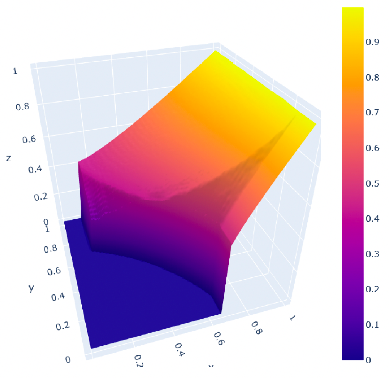
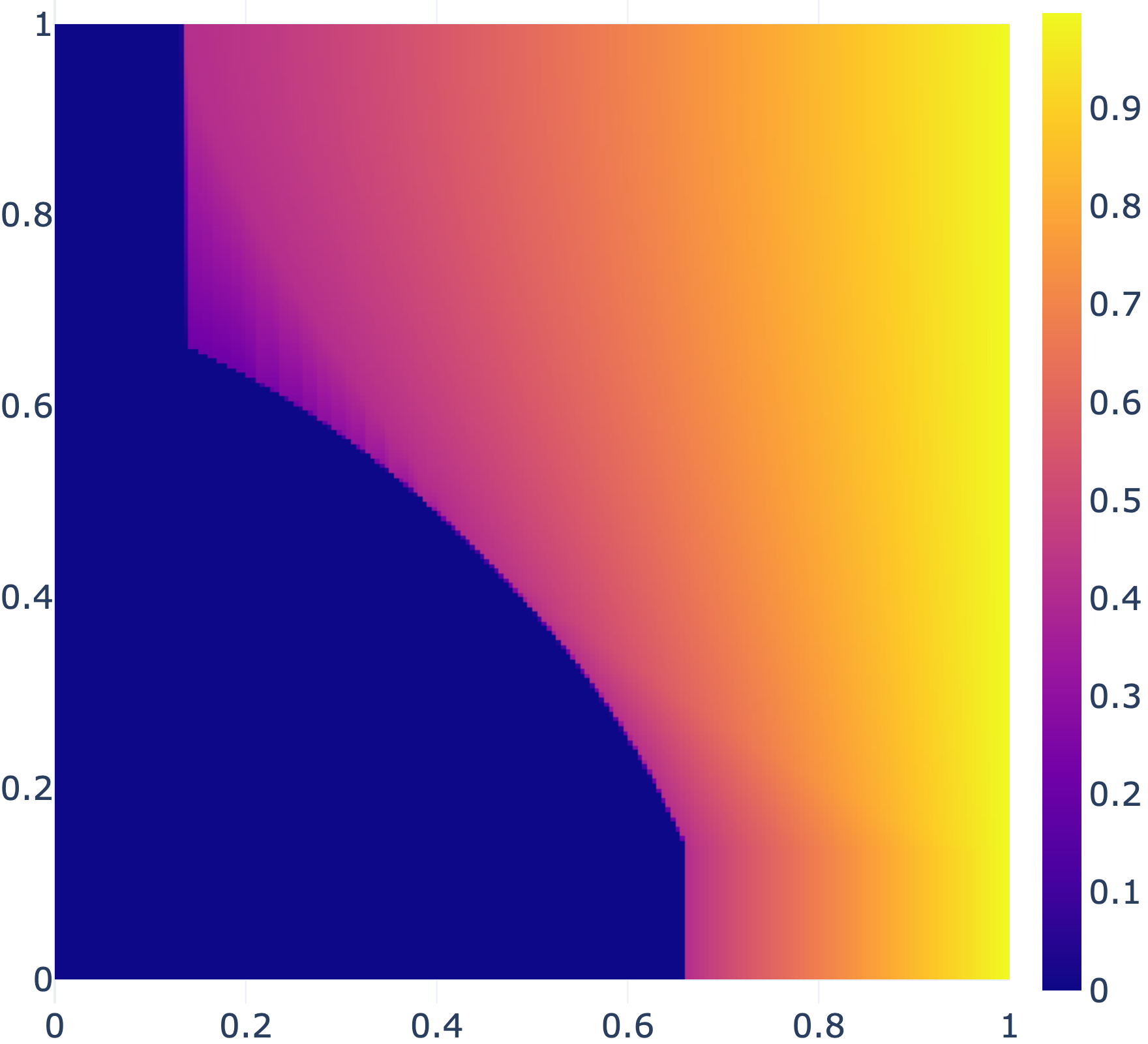
We conclude this section by presenting the result of numerical simulations for $n=m=2$ and the Lebesgue measure of $[0,1]^{2}$ ( figure 2 is taken from [14]). The detailed description of the algorithm can be found in [14]. The simulations indicate a complicated structure of the optimal mechanism and suggest that the optimal auction may not admit a closed-form solution even in this benchmark setting.

Refer to caption
Refer to caption
Figure 2: The probability to receive the first item as a function of bidder’s values $(x_{1},x_{2})$ in the optimal $2$-bidder $2$-item auction with i.i.d. values uniform on $[0,1]$.

5.3 Related questions, open problems

The above duality results raise many open question. We briefly list some of them.

  1. 1.

    Explicit solutions for dual problems.

    The closed-form solutions can be obtained in the setting of Example 1 (see [14], D). Here is a regular solution (for other examples, including singular solutions see [14]):

    $$c(x,y)=(c^{1}(x,y),c^{2}(x,y)),$$

    where

    $$c^{2}(x,y)=c^{1}(y,x)$$

    and

    $$c^{1}(x,y)=\begin{cases}0&(x,y)\in\mathcal{Z}\cup\mathcal{B}\\ 3x-2&(x,y)\in\mathcal{A}\\ \frac{3}{2}\bigl{(}x+y-\frac{4-\sqrt{2}}{3}\bigr{)}&(x,y)\in\mathcal{W},x\leq\frac{2}{3},y\leq\frac{2}{3}\\ \frac{9}{2}(1-x)\bigl{(}y-\frac{2-\sqrt{2}}{3}\bigr{)}\\ \quad\quad\quad\quad+3(x-\frac{2}{3})&(x,y)\in\mathcal{W},\frac{2}{3}\leq x\leq 1,\frac{2-\sqrt{2}}{3}\leq y\leq\frac{2}{3}\\ \frac{9}{4}\bigl{(}x-\frac{2-\sqrt{2}}{3}\bigr{)}^{2}&(x,y)\in\mathcal{W},\frac{2-\sqrt{2}}{3}\leq x\leq\frac{2}{3},\frac{2}{3}\leq y\leq 1\\ \frac{1}{2}+\frac{3}{2}\bigl{(}x-\frac{2}{3}\bigr{)}&(x,y)\in\mathcal{W},\frac{2}{3}\leq x\leq 1,\frac{2}{3}\leq y\leq 1\end{cases}$$

    Closed-form solutions are also available for the case of $n=1$. It this case the optimal vector field in the dual problem coincides with the Myersonian ironed virtual valuation.

  2. 2.

    Can the dual auctioneer’s problem for many bidders be interpreted as an optimal (weak) transportation problem?

    We will discuss this question in the following section. Let us also note that any Beckmann’s problem is always ([22], [6]) equivalent to an appropriate congested transport problem, which is a transportation problem on the infinite-dimensional space of curves (and it is a finite-dimensional transshipment problem only for the case when $\varphi_{i}$ are indicators of a segment, but this is not the case for $m>1$). Thus, converting the Beckmann’s problem into the congested transport problem, we get automatically a kind of infinite dimensional optimal transport problem. But it is not clear, whether this interpretation has some applications. In the other hand, we will see in the next section that functions $\varphi_{i}$ can be expelled from the dual formulation if we consider certain equivalent problem on $\overline{X}=X^{m}$.

  3. 3.

    Does there always exist a measure $\pi$ with finite variation giving minimum to the dual monopolist’s problem in Theorem 6?

    It was mistakenly claimed in [3] that such a measure always exists, but the proof contains a gap (the separating functional obtained as a limit can be the zero functional). In fact, this does not seem to be true for the general monopolist problem. But for the auctioneer’s problem this might be true. In particular, for $m=1$ bidder the majorising measure $\pi$ has the same variation as $\mu$ by Theorem 4.

    The measure $\pi$ always exists at least for sufficiently regular $\varphi$ and $\rho$, since it has representation $\pi=-{\rm div}(\nabla\varphi(\nabla u)\cdot\rho)$ and this always makes sense, because $\varphi$ and $u$ are convex. However, the variation of $\pi$ can be a priori infinite. In the other hand, we remark that $\pi$ has always finite $W^{1}_{l^{\infty}}$-norm for any $\varphi$, which is finite on $X$ and infinite outside of $X$. Indeed, taking a $1$-Lipschits (with respect to $l^{\infty}$-norm) function $v$ one gets

    $$\int_{X}vd\pi=\int_{X}\langle\nabla v,c\rangle\rho dx\leq\int_{X}|c|_{l^{1}}\rho dx.$$

    But the right-hand side is finite, because $\int_{X}\varphi^{*}(c)\rho dx<\infty$. Thus we get that the supremum of left-hand side is finite and by duality $\|\pi\|_{W^{1}_{l^{\infty}}}<\infty$. This, however, does not mean that $\pi$ has finite variation.

  4. 4.

    Regularity questions

    Does there always exist a regular vector field $c$ giving minimum in (30)? Regularity means that $\varsigma_{i}=0$. We do not know the answer. Picture 3 from [14] shows that $u$ does not look to be continuously differentiable, but $c$ and $\varphi_{i}$ seem to be smooth.

    Refer to caption
    Refer to caption
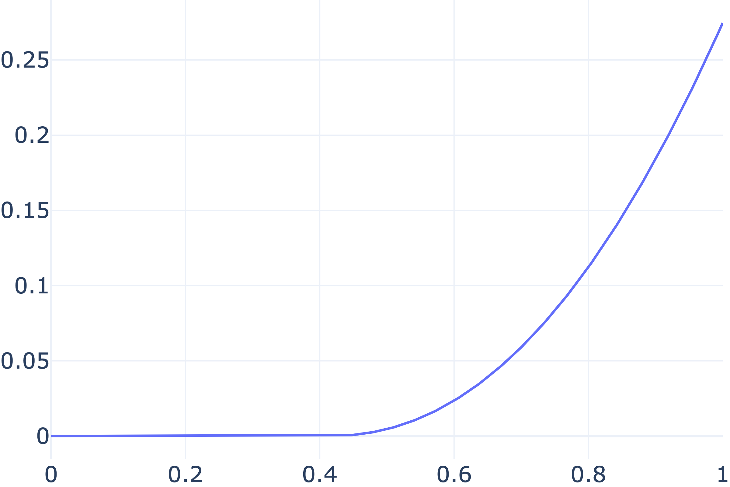
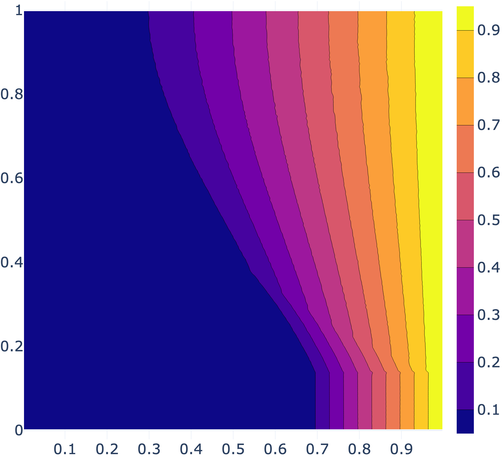
    Figure 3: The optimal solution to the dual problem: functions $\varphi_{1}=\varphi_{2}$ (left) and a contour plot of the first component of the vector field $c=(c_{1},c_{2})$ from Beckmann’s problem (right).

    It would be interesting to obtain any result on regularity of solutions in general case. Note that some regularity results for solutions of the monopolist’s problem has been obtained in [7].

6 Mechanism as a solution to a Beckmann’s problem with constraints

In this section we come back to the initial (unreduced) problem. Further we deal with the space

$$\overline{X}=X^{m}=([0,1]^{n})^{m}.$$

We will realize that a natural interpretation of the auction problem in terms of optimal transportation/ Beckmann’s transportation/linear duality leads to a $nm$-dimensional formulation. For part of the statements we omit the rigorous proofs but explain the main ideas.

6.1 Getting rid of functions $\varphi_{i}$

The dual functional suggested in Theorem 7 depends on vector field $c$ and functions $\varphi_{i}$. We show that functions $\varphi_{i}$ can be excluded from the functional, because the optimal choice of $\varphi_{i}$ is determined by distribution of $c$. Indeed, by the duality Theorem 7 the total revenue equals

$$m\cdot\inf_{c\in\mathcal{C}}\inf_{\footnotesize{\begin{array}[]{c}(\varphi_{i})_{1\leq i\leq n}\end{array}}}\sum_{i\in\mathcal{I}}\left(\int_{X}\varphi_{i}^{*}(|c_{i}|)\rho(x)\,\mathrm{d}x+\int_{0}^{1}\varphi_{i}\left(z^{m-1}\right)\,\mathrm{d}z\right),$$ (31)

where $\mathcal{C}$ is the set of vector fields satisfying

$$\int_{X}\bigl{(}\langle x,\nabla u\rangle-u\bigr{)}\rho dx\leq\int_{X}\langle\nabla u,c\rangle\rho dx,$$

for all $u\in\mathcal{U}$.

For a fixed $c$ and every $i$ the value

$$\inf_{\footnotesize{\begin{array}[]{c}(\varphi_{i})_{1\leq i\leq n}\end{array}}}\left(\int_{X}\varphi_{i}^{*}(|c_{i}|)\rho(x)\,\mathrm{d}x+\int_{0}^{1}\varphi_{i}\left(z^{m-1}\right)\ dz\right)=$$
$$\inf_{\footnotesize{\begin{array}[]{c}(\varphi_{i})_{1\leq i\leq n}\end{array}}}\left(\int\varphi_{i}^{*}(x_{i})\varrho_{i}(x_{i})\ dx_{i}+\frac{1}{m-1}\int_{0}^{1}\varphi_{i}(y_{i})y^{\frac{2-m}{m-1}}_{i}\ dy_{i}\right),$$

is the value of the dual transportation problem on $\mathbb{R}$ with cost function $x_{i}y_{i}$ and measures

$$\varrho_{i}(x_{i})dx_{i},\ \nu_{i},$$

where $\nu_{i}=\frac{1}{m-1}y^{\frac{2-m}{m-1}}_{i}\ dy_{i}$ and $\varrho_{i}(x_{i})dx_{i}$ is the distribution of $|c_{i}|$, i.e. image of $\rho$ under the mapping $|c_{i}|\colon\mathbb{R}^{n}\to\mathbb{R}_{+}$.

Hence by the one-dimensional Brenier theorem the corresponding optimal mapping has the form $T_{i}=(\varphi_{i}^{*})^{\prime}$ and satisfies

$$\int_{0}^{t_{i}}\varrho_{i}\,\mathrm{d}x_{i}=\frac{1}{m-1}\int_{0}^{T_{i}(t_{i})}y_{i}^{\frac{2-m}{m-1}}\,\mathrm{d}y_{i}=T^{\frac{1}{m-1}}_{i}(t_{i})$$

and the value of the dual transportational functional equals $\int x_{i}T_{i}(x_{i})\varrho_{i}\,\mathrm{d}x_{i}$.

Let $F_{i}(x_{i})=\int_{-\infty}^{x_{i}}\varrho_{i}(t)dt$. Hence

$$\int x_{i}T_{i}(x_{i})\varrho_{i}\,\mathrm{d}x_{i}=\int x_{i}F_{i}^{m-1}(x_{i})\varrho_{i}(x_{i})\,\mathrm{d}x_{i}=\frac{1}{m}\int x_{i}\varrho_{i}(x_{i})\,\mathrm{d}F_{i}^{m}(x_{i})$$

By the change of variables

$$\int x_{i}F_{i}^{m-1}(x_{i})\varrho_{i}(x_{i})\,\mathrm{d}x_{i}=\int_{X}|c_{i}|F_{i}^{m-1}(|c_{i}|)\rho dx$$

and we get the following result:

Proposition 2.

The auctioneer’s problem is equivalent to the minimization problem

$$\sum_{1\leq i\leq n}\int_{X}|c_{i}|F_{i}^{m-1}(|c_{i}|)\rho dx\to\min,\ c\in\mathcal{C},$$

where $F_{i}(t)=\int_{\{x:|c_{i}|(x)\leq t\}}\rho dx.$

Next we note that

$$\int x_{i}F_{i}^{m-1}(x_{i})\varrho_{i}(x_{i})\,\mathrm{d}x_{i}=\frac{1}{m}\mathbb{E}\left[\max_{1\leq j\leq m}x_{i,j}\right]$$

where $x_{i,j}\in X$ are independent random variables with distribution $\varrho_{i}$.

Thus we obtain the following result

Proposition 3.

The value of the auctioneer’s problem is

$$\inf_{P}\mathbb{E}^{P}\sum_{1\leq i\leq n}\max(x_{i,1},x_{i,2},\cdots,x_{i,m}),$$

where for every fixed $i$ the random variables $x_{i,j},1\leq j\leq m$ are independent and have distribution $Pr_{i}P$. The infimum is taken over distributions on $\mathbb{R}^{n}$ satisfying the following property: there exists a vector field $c\in\mathcal{C}$ with distribution $Pr_{i}P$.

6.2 Beckmann’s problem on $X^{m}$ with linear constraints

In this subsection we get an equivalent formulation of the dual auction design problem on the space $\overline{X}=X^{m}$.

In what follows we denote ${x}_{j}=(x_{1,j},\cdots,x_{n,j})$. As before, we equip $\overline{X}$ with the product measure

$$\overline{\rho}(x)dx=\bigotimes_{j=1}^{m}\rho({x}_{j})d{x}_{j}$$

and the suitable norm

$$|x|_{\overline{X}}=\sum_{1\leq i\leq n}\max(|x_{i,1}|,|x_{i,2}|,\cdots,|x_{i,m}|).$$

For every vector field

$$c=(c_{1},\cdots,c_{n})$$

let us define the extended vector field

$$\overline{c}({x}_{1},\cdots,{x}_{m})=(c({x}_{1}),\cdots,c({x}_{m})).$$ (32)

Note that

$${\rm div}_{\overline{\rho}}\overline{c}=\sum_{j=1}^{m}\rho({x}_{1})d{x}_{1}\times\cdots\times{\rm div}_{\rho}c({x}_{j})\times\cdots\rho({x}_{m})d{x}_{m}.$$

These observation together with Proposition 3 leads to the following conclusion

Proposition 4.

(Auction’s design problem as a Beckmann’s problem with linear constraints) The auction design problem is equivalent to the following minimization problem:

$$\inf_{\pi\succeq\mu,\overline{c}}\int_{\overline{X}}|\overline{c}|_{\overline{X}}\overline{\rho}({x})d{x},$$

where $\overline{c}$ satisfies

  1. 1.
    $${\rm div}_{\overline{\rho}}\overline{c}=-\overline{\pi},$$
    $$\overline{\pi}=\sum_{j=1}^{m}\rho({x}_{1})d{x}_{1}\times\cdots\times\pi(d{x}_{j})\times\cdots\rho({x}_{m})d{x}_{m},$$ (33)
  2. 2.

    $\overline{c}$ has the form (32).

6.3 Dual Beckmann’s problem with linear constraints

Let us consider a general Beckmann’s problem with linear constraints. Let $\varphi$ be a convex function on $\overline{X}$ with values in $\mathbb{R}\cup\{+\infty\}$ and $L\subset L^{2}(\overline{\rho}dx)$ be a linear space of vector fields with values in $\mathbb{R}^{mn}$. Let us denote by $L^{\bot}$ the corresponding space of orthogonal ( in the $L^{2}(\overline{\rho}dx)$-sense) vector fields

$$c\in L^{\bot}\Longleftrightarrow\int_{\overline{X}}\langle c,F\rangle\overline{\rho}dx=0\ \ \forall F\in L.$$

Consider the maximization problem

$$\sup_{v\in C^{1}_{b}(\overline{X}),F\in L}\Bigl{(}\int_{\overline{X}}vd\overline{\pi}-\int_{\overline{X}}\varphi(\nabla v+F)\overline{\rho}dx\Bigr{)},$$

where $C^{1}_{b}(\overline{X})$ is the set of continuously differentiable functions on $\overline{X}$ and $\overline{\pi}$ is a measure with finite variation satisfying $\overline{\pi}(\overline{X})=0$.

The following result is a generalization of Theorem 5. We omit the rigorous proof, but explain its main idea.

Theorem 9.
$$\sup_{v\in C^{1}_{b}({\overline{X}}),F\in L}\Bigl{(}\int_{\overline{X}}vd\overline{\pi}-\int_{\overline{X}}\varphi(\nabla v+F)\overline{\rho}dx\Bigr{)}=\inf_{c\in L^{\bot},-{\rm div}(c\cdot\overline{\rho})=\overline{\pi}}\int_{\overline{X}}\varphi^{*}(c)\overline{\rho}dx.$$

Weak duality $\sup\leq\inf$ can be proved in the standard way:

$\displaystyle\int_{\overline{X}}vd\overline{\pi}-\int_{\overline{X}}\varphi(\nabla v+F)\overline{\rho}dx=-\int_{\overline{X}}vd{\rm div}(c\cdot\overline{\rho})-\int_{\overline{X}}\varphi(\nabla v+F)\overline{\rho}dx$
$\displaystyle=\int_{\overline{X}}\langle\nabla v,c\rangle\overline{\rho}dx-\int_{\overline{X}}\varphi(\nabla v+F)\overline{\rho}dx=\int_{\overline{X}}\langle\nabla v+F,c\rangle\overline{\rho}dx-\int_{\overline{X}}\varphi(\nabla v+F)\overline{\rho}dx$
$\displaystyle\leq\int_{\overline{X}}\varphi^{*}(c)\overline{\rho}dx.$

Assuming that $\varphi$ is sufficiently regular, by the standard variational arguments we obtain that the maximum point $(v_{0},F_{0}),F_{0}\in L$ of $\int_{\overline{X}}vd\overline{\pi}-\int_{\overline{X}}\varphi(\nabla v+F)\overline{\rho}dx$ satisfies

$${\rm div}(\nabla\varphi(\nabla v_{0}+F_{0})\rho)=-\overline{\pi},\ \ \nabla\varphi(\nabla v_{0}+F_{0})\in L^{\bot}.$$

Thus the field $c_{0}=\nabla\varphi(\nabla v_{0}+F_{0})$ is admissible for the dual problem. Hence

$\displaystyle\int_{\overline{X}}v_{0}d\overline{\pi}-\int_{\overline{X}}\varphi(\nabla v_{0}+F_{0})\overline{\rho}dx=-\int_{\overline{X}}v_{0}{\rm div}(c_{0}\cdot\overline{\rho})-\int_{\overline{X}}\varphi(\nabla v_{0}+F_{0})\overline{\rho}dx$
$\displaystyle=\int_{\overline{X}}\langle\nabla v_{0},c_{0}\rangle\overline{\rho}dx-\int_{\overline{X}}\varphi(\nabla v_{0}+F_{0})\overline{\rho}dx$
$\displaystyle=\int_{\overline{X}}\langle\nabla v_{0}+F_{0},\nabla\varphi(\nabla v_{0}+F_{0})\rangle\overline{\rho}dx-\int_{\overline{X}}\varphi(\nabla v_{0}+F_{0})\overline{\rho}dx$
$\displaystyle=\int_{\overline{X}}\varphi^{*}(\nabla\varphi(\nabla v_{0}+F_{0}))\overline{\rho}dx.$

Thus we get a formal proof of the desired identity.

In particular, for

$$\varphi^{*}=|\cdot|_{\overline{X}}$$

and a linear space $L$ of vector fields we consider the Beckmann’s problem

$$\int_{\overline{X}}|c|_{\overline{X}}\overline{\rho}dx\to\min$$
$$-{\rm\mathrm{div}}_{\overline{\rho}}c=\overline{\pi},$$

with constraint $\int_{\overline{X}}\langle c,F\rangle\overline{\rho}dx=0,\ \forall F\in L$ for a linear space $L$. The dual problem takes the form

$$\sup_{v\in C^{1}_{b}(\overline{X}),F\in L}\Bigl{(}\int_{\overline{X}}vd\overline{\pi}-\int_{\overline{X}}\varphi(\nabla v+F)\overline{\rho}dx\Bigr{)},$$

where

$$\varphi(x)=\delta_{\|x\|_{\overline{X}^{\circ}}\leq 1}=(\|\cdot\|_{\overline{X}})^{*}.$$

Clearly, the problem is equivalent to the maximization problem

$$\sup_{v\in Lip(|\cdot|_{\overline{X}},L)}\int_{\overline{X}}vd\overline{\pi},$$

where $Lip(|\cdot|_{\overline{X}},L)$ is the set of functions satisfying inequality $|\nabla v+F|_{{\overline{X}^{\circ}}}\leq 1$ for some $F\in L$. The duality theorem takes the form:

Theorem 10.
$$\sup_{v\in Lip(|\cdot|_{\overline{X}},L)}\int_{\overline{X}}vd\overline{{\pi}}=\inf_{c\in L^{\bot},-{\rm div}_{\overline{\rho}}c=\overline{\pi}}\int_{\overline{X}}|c|_{\overline{X}}\overline{\rho}dx$$

Our next aim is to relate the dual Beckmann’s problem with constraint to the optimal transshipment problem.

Lemma 1.

Let $F$ be a continuous vector field. Set:

$$d_{F}(x,y)=\sup_{v:|\nabla v+F|_{\overline{X}^{\circ}\leq 1}}\bigl{(}v(x)-v(y)\bigr{)}.$$

Then for a differentiable function $v$ the following properties are equivalent:

  1. 1.

    $|\nabla v+F|_{\overline{X}^{\circ}}\leq 1$

  2. 2.

    For all $x,y$ one has:

    $$v(x)-v(y)\leq d_{F}(x,y).$$

    Equivalently $-d_{F}(y,x)\leq v(x)-v(y)\leq d_{F}(x,y).$

Proof.

Clearly 1) $\Longrightarrow$ 2). Assume that $v$ satisfies 2). Then any differentiable function $w$ with property $|\nabla w(x)+F(x)|_{\overline{X}^{\circ}}\leq 1$ satisfies the obvious inequality:

$$|w(y)-w(x)+\langle F(x),y-x\rangle|\leq|y-x|_{\overline{X}}+o(|y-x|)$$

for all $y$ form a small neighborhood of $x$. In particular, we get

$$d_{F}(y,x)+\langle F(x),y-x\rangle\leq|y-x|_{\overline{X}}+o(|y-x|).$$ (34)

Assume that at some point $x_{0}$ one has $|\nabla v(x_{0})+F(x_{0})|_{\overline{X}^{\circ}}>1$. This means that for a vector $e$ with $|e|_{\overline{X}}=1$, one has: $\langle e,\nabla v(x_{0})+F(x_{0})\rangle>1$. In particular, for small values of $t$

$$v(x_{0}+te)-v(x_{0})+\langle F(x_{0}),te\rangle=\langle te,\nabla v(x_{0})+F(x_{0})\rangle+o(t)>t+o(t)=|te|_{\overline{X}}+o(t).$$

Thus one has by 2)

$$d_{F}(x_{0}+te,x_{0})+\langle F(x_{0}),te\rangle\geq v(x_{0}+te)-v(x_{0})+\langle F(x_{0}),te\rangle\geq|te|_{\overline{X}}+o(t).$$

Consequently, inequality (34) is false for $x=x_{0}$, $y=x_{0}+te$ and sufficiently small $t$. We get a contradiction. ∎

Applying the well-known duality for the optimal transshipment problem we get the following

$\displaystyle\sup_{v\in Lip(|\cdot|_{\overline{X}},L)}\int_{\overline{X}}vd\overline{{\pi}}=\sup_{v,F\in L:|v+\nabla F|_{\overline{X}^{\circ}}\leq 1}\int_{\overline{X}}vd\overline{{\pi}}$
$\displaystyle=\sup_{F\in L}\Bigl{(}\sup_{v:v(x)-v(y)\leq d_{F}(x,y)}\int_{\overline{X}}vd\overline{\pi}\Bigr{)}$
$\displaystyle=\sup_{F\in L}\Bigl{(}\inf_{\gamma:{\rm Pr}_{1}\gamma-{\rm Pr}_{2}\gamma=\overline{\pi}}\int_{\overline{X}\times\overline{X}}d_{F}(x,y)d\gamma\Bigr{)}.$

Finally we obtain that the dual Beckmann’s problem with linear constraints is related to the transshipment problem in the following way

Theorem 11.

(Relation to the optimal transshipment problem)

$$\inf_{c\in L^{\bot},-{\rm div}_{\overline{\rho}}c=\overline{\pi}}\int_{\overline{X}}|c|_{\overline{X}}\overline{\rho}dx=\sup_{F\in L}\Bigl{(}\inf_{\gamma:{\rm Pr}_{1}\gamma-{\rm Pr}_{2}\gamma=\overline{\pi}}\int_{\overline{X}\times\overline{X}}d_{F}(x,y)d\gamma\Bigr{)}.$$

6.4 Applications to symmetric mechanisms

In what follows

$$|{x}|_{\overline{X}}=\sum_{1\leq i\leq n}\max(|x_{i,1}|,|x_{i,2}|,\cdots,|x_{i,m}|),$$

$|\cdot|_{\overline{X}^{\circ}}$ is the dual norm. We consider space of vector fields having the form

$$\overline{c}({x}_{1},\cdots,{x}_{m})=(c({x}_{1}),\cdots,c({x}_{m})).$$ (35)

Recall that a function $f$ symmetric, if it is symmetric with respect to any permutation $\sigma$ of coordinates

$$T_{\sigma}(x_{1},\cdots,x_{m})=(x_{\sigma(1)},\cdots,x_{\sigma(m)}).$$

A field $F\colon\overline{X}\to\mathbb{R}^{nm}$ is called symmetric, if

$$F\circ T_{\sigma}(x)=T_{\sigma}(F(x)).$$

This space of symmetric vector fields will be denoted by Ls​y​msuperscriptπΏπ‘ π‘¦π‘šL^{sym}.

Let $L$ be the space

$$L=L_{1}+L_{2},$$

where

  • β€’

    L1subscript𝐿1L_{1} is the space of fields

    $$F\colon\overline{X}\to\overline{X},$$
    $$F=(F_{1},F_{2},\cdots,F_{m}),\ F_{j}=(F_{1j},\cdots,F_{nj}),$$

    such that for every $k$ the conditional expectation of $F_{k}$ with respect to $x_{k}$ vanishes

    𝔼ρ¯​(Fk|xk)=∫∏jβ‰ kXjFkβ€‹βˆjβ‰ kρ​(xi)​d​xj=0superscriptπ”ΌΒ―πœŒconditionalsubscriptπΉπ‘˜subscriptπ‘₯π‘˜subscriptsubscriptproductπ‘—π‘˜subscript𝑋𝑗subscriptπΉπ‘˜subscriptproductπ‘—π‘˜πœŒsubscriptπ‘₯𝑖𝑑subscriptπ‘₯𝑗0\mathbb{E}^{\overline{\rho}}(F_{k}|{x}_{k})=\int_{\prod_{j\neq k}X_{j}}F_{k}\prod_{j\neq k}\rho({x}_{i})d{x}_{j}=0
  • β€’
    L2={vector fields,Β L2​(ρ¯​d​x)-orthogonal to symmetric fields}subscript𝐿2vector fields,Β L2(ρ¯dx)-orthogonal to symmetric fieldsL_{2}=\{\mbox{vector fields, $L^{2}(\overline{\rho}d{x})$-orthogonal to symmetric fields}\}

The following lemma in obvious.

Lemma 2.

The space of fields satisfying (35) coincides with the space $L^{\bot}$.

We get immediately from this Lemma and Proposition 4. the value of auctioneer’s problem coincides with

$$\inf_{\pi\succeq\mu}\sup_{v\in Lip(|\cdot|_{\overline{X}},L)}\int_{\overline{X}}vd\overline{{\pi}},$$

where $\overline{\pi}$ is defined by (33). Note, however, that the space $L$ is not the most convenient space to work with, because it contains $L_{2}$. In fact, we can do additional symmetrization, since $\overline{\pi}$ is symmetric with respect to any $T_{\sigma}$. Let $v_{0},F_{0}$ be a solution to maximization problem $\sup_{v\in Lip(|\cdot|_{\overline{X}},L)}\int_{\overline{X}}vd\overline{{\pi}}$. and vs​y​m,Fs​y​msuperscriptπ‘£π‘ π‘¦π‘šsuperscriptπΉπ‘ π‘¦π‘šv^{sym},F^{sym} be obtained from $v_{0},F_{0}$ by symmetrization:

vs​y​m=1m!β€‹βˆ‘Οƒv0∘TΟƒ,Fs​y​m=1m!β€‹βˆ‘ΟƒTσ​(F0∘TΟƒ).formulae-sequencesuperscriptπ‘£π‘ π‘¦π‘š1π‘šsubscript𝜎subscript𝑣0subscriptπ‘‡πœŽsuperscriptπΉπ‘ π‘¦π‘š1π‘šsubscript𝜎subscriptπ‘‡πœŽsubscript𝐹0subscriptπ‘‡πœŽv^{sym}=\frac{1}{m!}\sum_{\sigma}v_{0}\circ T_{\sigma},\ F^{sym}=\frac{1}{m!}\sum_{\sigma}T_{\sigma}(F_{0}\circ T_{\sigma}).

Then by symmetry of $\overline{\pi}$ one has

$$\int_{\overline{X}}v_{0}d\overline{\pi}=\int_{\overline{X}}v^{\mathrm{sym}}d\overline{\pi}.$$

In addition, since $\nabla\bigl{(}v_{0}\circ T_{\sigma}\bigr{)}=T_{\sigma}(\nabla v\circ T_{\sigma})$, one gets $(\nabla v_{0})^{\mathrm{sym}}=(\nabla v^{\mathrm{sym}}).$ Using symmetry of $|\cdot|^{\circ}_{X}$ and its convexity, we get immediately that $v^{\mathrm{sym}},F^{\mathrm{sym}}$ satisfy the same constraint $|v^{\mathrm{sym}}+F^{\mathrm{sym}}|_{\overline{X}^{\circ}}\leq 1$. Note that $F^{\mathrm{sym}}\in L_{1}\cap L^{\mathrm{sym}}$. Thus we obtain the following result:

Proposition 5.

The value of auctioneer’s problem equals

$$\sup_{v\in Lip^{sym}(|\cdot|_{\overline{X}},L_{1}\cap L^{\mathrm{sym}})}\int_{\overline{X}}vd\overline{{\pi}},$$

where $Lip^{sym}(|\cdot|_{\overline{X}},L_{1}\cap L^{\mathrm{sym}})$ is the set of symmetric functions satisfying $|\nabla v+F|_{\overline{X}^{\circ}}\leq 1$ for some F∈L1∩Ls​y​m𝐹subscript𝐿1superscriptπΏπ‘ π‘¦π‘šF\in L_{1}\cap L^{sym}.

We get by Theorem 11:

Theorem 12.

(Auctions with $m>1$ bidders and transshipment problem) The value of the auction design problem equals

supF∈L1∩Ls​y​m(infΞ³:Pr1β€‹Ξ³βˆ’Pr2​γ=π¯,Ο€βͺ°ΞΌβˆ«XΒ―Γ—XΒ―dF​(x,y)​𝑑γ).subscriptsupremum𝐹subscript𝐿1superscriptπΏπ‘ π‘¦π‘šsubscriptinfimum:𝛾formulae-sequencesubscriptPr1𝛾subscriptPr2π›ΎΒ―πœ‹succeeds-or-equalsπœ‹πœ‡subscript¯𝑋¯𝑋subscript𝑑𝐹π‘₯𝑦differential-d𝛾\sup_{F\in L_{1}\cap L^{sym}}\Bigl{(}\inf_{\gamma:{\rm Pr}_{1}\gamma-{\rm Pr}_{2}\gamma=\overline{\pi},\pi\succeq\mu}\int_{\overline{X}\times\overline{X}}d_{F}(x,y)d\gamma\Bigr{)}.

Here

$$d_{F}(x,y)=\sup_{v:|\nabla v+F|_{\overline{X}^{\circ}\leq 1}}\bigl{(}v(x)-v(y)\bigr{)},$$

where the supremum is taken over symmetric $v$ and F∈L1∩Ls​y​m𝐹subscript𝐿1superscriptπΏπ‘ π‘¦π‘šF\in L_{1}\cap L^{sym}

We conclude this subsection with a theorem which relates symmetric optimal mechanisms to the dual Beckmann’s problem.

Theorem 13.

(Symmetric mechanism as a solution to the dual Beckmann’s problem) Let $\pi,v_{0},F_{0}$ be a solution to optimization problem

$$\inf_{\pi\succeq\mu}\sup_{v\in Lip^{sym}(|\cdot|_{\overline{X}},L_{1}\cap L^{sym})}\int_{\overline{X}}vd\overline{{\pi}}.$$

Then the couple $(P_{0},T_{0})$, where

$$P_{0}({x})=\nabla v_{0}({x})+F_{0}({x}),$$
$$(T_{0})_{j}({x})=\langle{x}_{j},(P_{0})_{j}({x})\rangle-v_{0}({x}),$$

is a solution to the (unreduced) auctioneer’s problem, i.e. $(P_{0},T_{0})$ is the optimal, symmetric, feasible mechanism, satisfying (8), (7).

In particular, the total revenue equals

$$\sum_{j=1}^{m}(T_{0})_{j}({x})=\langle{x},P_{0}({x})\rangle-mv_{0}({x}).$$

Taking conditional expectation of $v_{0}$ we obtain a solution to the reduced problem:

$$\mathbb{E}^{\overline{\rho}}(v_{0}|{x}_{j})=u_{0}({x}_{j}).$$

Applying conditional expectation with respect to ${x}_{j}$ to $((P_{0})_{j},(T_{0})_{j})$ and taking into account that $\mathbb{E}^{\overline{\rho}}((F_{0})_{j}|{x}_{j})=0$, we get the known relation for the reduced mechanism $(\overline{P}_{0},\overline{T}_{0})$ on $X$:

$$\overline{P}_{0}=\nabla u_{0}$$
$$\overline{T}_{0}(x)=\langle x,\nabla u_{0}(x)\rangle-u_{0}(x).$$

References

  • [1] Backhoff-VeraguasΒ J., Pammer G., "Applications of weak transport theory." Bernoulli 28 (1) 370 - 394, February 2022.
  • [2] Beckmann M., A continuous model of transportation, Econometrica: Journal of the Econometric Society, 1952, 643–660.
  • [3] BogachevΒ T.V., Kolesnikov A.V., On the Monopolist Problem and Its Dual, Mathematical Notes, 2023, Volume 114, Issue 2, Pages 147–158.
  • [4] Bogachev V.I., Kolesnikov A.V., The Monge–Kantorovich problem: achievements, connections, and perspectives, Russian Mathematical Surveys, 67 (5), 2012, p. 785–890.
  • [5] Border K. C. (2007), β€œReduced Form Auctions Revisited,” Economic Theory 31, 167–181.
  • [6] Brasco L., Petrache M. A Continuous Model of Transportation Revisited. J Math Sci 196, 119–137 (2014).
  • [7] Carlier G., Lachand-Robert T., Regularity of solutions for some variational problems subject to a convexity constraint, Commun. Pure Appl. Anal. 2001, 54 (5), 583–594.
  • [8] ChonΓ© P., Kramarz F., Matching Workers’ Skills and Firms’ Technologies: From Bundling to Unbundling, Preprint, 2021
  • [9] Daskalakis C., Deckelbaum A., Tzamos, C., Strong Duality for a Multiple-Good Monopolist, Econometrica, 2017, 85(3), 735–767, (2017)
  • [10] Figalli A., Kim Y.-H., McCann R.-J. When is multidimensional screening a convex program?, Journal of Economic Theory, 146(2), 454–478, (2011).
  • [11] Galichon A. Optimal transport methods in economics. Princeton University Press, Princeton, 2016; xii+170 p.
  • [12] Gozlan N., Roberto C., Samson P.-M., Tetali P. Kantorovich duality for general transport costs and applications. J. Funct. Anal. 2017. V. 273, β„–11. P. 3327–3405.
  • [13] Hart S., Reny P., Implementation of reduced form mechanisms: a simple approach and a new characterization, Economic Theory Bulletin, 2015, 3(1), 1–8.
  • [14] KolesnikovΒ A.V., SandomirskiyΒ F., TsyvinskiΒ A., ZiminΒ A.P., Beckmann’s approach to multi-item multi-bidder auctions, https://arxiv.org/pdf/2203.06837.pdf
  • [15] Manelli A.M., Vincent D.R., Bundling as an optimal selling mechanism for a multiple-good monopolist. Journal of Economic Theory, 127(1):1–35, 2006.
  • [16] Matthews S. A. (1984), β€œOn the Implementability of Reduced Form Auctions,” Econometrica 52, 1519–1522.
  • [17] McCann, R., Zhang, K.S., On Concavity of the Monopolist’s Problem Facing Consumers with Nonlinear Price Preferences, Communication on pure and applied mathematics, 72(7), 1386–1423, (2019).
  • [18] McCann, R., Zhang, K.S., A duality and free boundary approach to adverse selection (working paper).
  • [19] Mussa M., Rosen S.,"Monopoly and Product Quality," Journal of Economic Theory, (1978), 18, 301-317.
  • [20] Myerson R.B.,. Optimal auction design. Mathematics of operations research, 6(1): 58–73, 1981.
  • [21] Rochet J.-P., Choné P., Ironing, Sweeping, and Multidimensional Screening. Econometrica, 1998, 66(4), 783–826.
  • [22] Santambrogio F., Optimal transport for applied mathematicians, BirkΓ€user, NY, 2015.
  • [23] Villani C. Topics in optimal transportation. Amer. Math. Soc. Providence, Rhode Island, 2003; xvi+370Β p.