PySCIPOpt-ML: Embedding Trained Machine Learning Models into Mixed-Integer Programs

Abstract

A standard tool for modelling real-world optimisation problems is mixed-integer programming (MIP). However, for many of these problems there is either incomplete information describing variable relations, or the relations between variables are highly complex. To overcome both these hurdles, machine learning (ML) models are often used and embedded in the MIP as surrogate models to represent these relations. Due to the large amount of available ML frameworks, formulating ML models into MIPs is highly non-trivial. In this paper we propose a tool for the automatic MIP formulation of trained ML models, allowing easy integration of ML constraints into MIPs. In addition, we introduce a library of MIP instances with embedded ML constraints. The project is available at https://github.com/Opt-Mucca/PySCIPOpt-ML.

1 Introduction and Related Work

Many problems coming from real-world applications can be modelled using Mixed-Integer Programming (MIP). They can be expressed as

$$\underset{x\in\mathbb{R}^{n}}{\text{min}} f_{0}(x)$$ (P)

s.t. $$f_{i}(x)\leq 0,\ \forall i\in[m],$$

$$x_{i}\in\mathbb{Z},\ \forall i\in\mathcal{I},$$

where each $f_{i}:\mathbb{R}^{n}\rightarrow\mathbb{R},i=0,\dots,m$ is continuous and $\mathcal{I}\subseteq[n]$ denotes the index set of the integer-constrained variables. Due to its ability to represent complex systems and decision-making processes across various industries, MIP has become a standard tool to solve optimisation problems arising in real-world applications.

A common challenge of finding a suitable MIP formulation (P) of a system is the presence of unknown or highly complex relationships. This poses a problem since traditional MIP approaches rely on precise definitions of constraints and the objective function. To address this challenge, Machine Learning (ML) predictors are often used to approximate these relationships and are then embedded in (P) as surrogate models. To embed a trained ML predictor $g:\mathbb{R}^{n}\rightarrow\mathbb{R}$, it must first be formulated as a MIP, before it can be added to (P). However, with the growing popularity and accessibility of different frameworks [1, 2, 3, 4, 5], automatically formulating trained ML models coming from these different architectures into MIPs has become a highly non-trivial, yet necessary task.

Contribution.

In this paper, we present PySCIPOpt-ML, an open-source tool for the automatic formulation of trained ML predictors as MIPs. By directly interfacing with a broad range of commonly used ML frameworks, PySCIPOpt-ML allows for the easy integration of ML constraints into MIPs, which can then be solved by the state-of-the-art open-source solver SCIP [6]. The package supports various models from Scikit-Learn [2], XGBoost [3], LightGBM [4], and PyTorch [5], making it a general tool to easily optimise MIPs with embedded ML constraints (see Figure 1). To represent predictors as MIPs, we use formulations that prioritise numerical stability to enhance solution robustness. In addition, we introduce an expandable library of MIP instances with embedded ML constraints based on real-world data.

To summarise, our contributions are the following:

1. We introduce the Python package PySCIPOpt-ML, which directly interfaces various ML frameworks with the open-source solver SCIP (see Section 2).

2. We utilise MIP formulations prioritising numerical stability, especially when solving with SCIP (see Section 3).

3. We introduce a new library of MIP instances with embedded ML constraints called SurrogateLIB, as well as the corresponding instance generators (see Section 4).

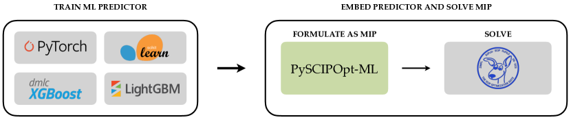
Figure 1: How trained ML predictors can be automatically formulated as MIPs and embedded in an optimisation problem using our Python package PySCIPOpt-ML.

Related Work.

In recent years, more and more industries have leveraged ML frameworks to approximate unknown or complex relationships in optimisation problems. For instance, ML predictors have been used to optimise cancer treatment plans [7], minimise energy consumption [8], and in the design of energy systems [9]. Embedded ML predictors have also been used in the optimisation of gas production and water management systems [10], as well as in the optimisation of retail prices [11] and locations [12], to name only a few examples. For surveys of embedded ML models through surrogate optimisation, see [13, 14, 15].

The increasing demand for embedding ML predictors into MIPs has motivated the development of various tools for automatic integration. The commercial MIP solver Gurobi released the Python package Gurobi Machine Learning [16], which integrates trained regression models into optimisation problems that can then be solved with Gurobi. Another package that relies on Gurobi is Janos [17], which supports linear and logistic regression, as well as neural networks with rectified linear unit (ReLU) activation functions. ENTMOOT [18] focuses on representing gradient-boosted tree models from LightGBM. On the other hand, reluMIP [19] allows the user to integrate ReLU neural networks trained with TensorFlow [1] within optimisation problems modelled with either Pyomo [20] or Gurobi. OMLT [21] focuses on embedding neural networks and gradient-boosted trees via the general MIP modelling framework Pyomo [20] and the general purpose ML interface ONNX.

While many of these packages focus on supporting specific types of predictors, PySCIPOpt-ML allows the user to embed a wide variety of predictors. Specifically, for both regression and classification tasks, neural networks with various activation functions, linear and logistic regression models, decision trees, gradient boosted trees, and random forests.

2 About the Package

PySCIPOpt-ML directly interfaces with the popular ML frameworks Scikit-Learn [2], XGBoost [3], LightGBM [4], and PyTorch [5]. Each framework allows the user to train ML predictors of different types, all of which can be embedded into a MIP by our package. A detailed overview of what PySCIPOpt-ML supports is given in Table 1.

ML Predictor	PyTorch	Scikit-Learn	LightGBM	XGBoost
Decision Trees	-	R+C	R+C	R+C
Gradient Boosted Trees	-	R+C	R+C	R+C
Random Forests	-	R+C	R+C	R+C
Neural Networks	R+C	R+C	-	-
Linear Regression	-	R	-	-
Logistic Regression	-	R+C	-	-
Partial Least Squares	-	R	-	-

Table 1: Overview of ML predictors coming from different ML frameworks supported by PySCIPOpt-ML. “R” indicates that (multi-)regression is supported and “C” denotes the support of (multi-)classification. “-” show predictors not supported by a framework and thus not supported by PySCIPOpt-ML.

An advantage of PySCIPOpt-ML is that it seamlessly joins all parts of the modelling, training, and optimisation processes. At no point is there a need to export the ML predictor or MIP model into some intermediary language. A central function (add_predictor_constr()) acts as the main interface between the ML frameworks training the predictor and the solver SCIP solving the problem. To create and solve a MIP problem with an embedded ML predictor, the user must only do the following:

1. Define the optimisation problem, scip_model, by first adding the explicit constraints and objective function.

2. Given data (input_data,output_data), choose which predictor should be trained and embed the trained predictor automatically in the optimisation problem as a constraint. This is done by simply calling:

   $${\texttt{add\_predictor\_constr(scip\_model, predictor, input\_data, output\_data)}}.$$

3. Solve the updated scip_model with SCIP.

In summary, PySCIPOpt-ML helps to easily create, embed, and solve optimisation problems with ML surrogate models and spares the user from navigating multiple platforms at the same time.

3 MIP Formulations of ML Predictors

To embed an ML predictor in a MIP, we first need to represent the predictor itself as a MIP. The formulation of the predictor has a significant effect on the ability to efficiently optimise the larger optimisation problem. There has been a substantial amount of work on determining the best performing formulations for popular ML predictors. In particular, neural networks with ReLU activation functions [22, 23, 24, 25] and ensemble based methods that use decision trees [26, 18, 27, 16], have received a lot of attention in the past. Often, the most natural formulation of these predictors involves quadratic constraints. Due to performance issues, however, formulations that utilise big-M, indicator, and SOS constraints are in general preferred.

3.1 Neural Networks

The current standard MIP formulation for feed forward neural networks with ReLU activation functions is to use big-M constraints [22, 24, 21]. These formulations are prone to numerical issues when the bounds on the input are large, and thus benefit greatly from tighter bounds. For this reason, either feasibility based or optimality based bound tightening is typically performed prior to optimisation [22, 21]. It is therefore important that the user specifies bounds on the variables of the wider optimisation problem. Since this is not always possible, PySCIPOpt-ML utilises a SOS1-based formulation to represent ReLU activation functions. By doing so, we aim to maintain numerical stability even in the absence of tight variable bounds, as the validity of the constraints can be enforced by branching [28].

Consider a single neuron in a fully connected layer $k$. Let $x\in\mathbb{R}^{n}$ be the output of the previous layer $k-1$, $y\in\mathbb{R}$ be the output of the given neuron, $w\in\mathbb{R}^{n}$ and $b\in\mathbb{R}$ be the weights and bias connecting the previous layer to the neuron, and $s\in\mathbb{R}_{\geq 0}$ be some slack variable. We use the following formulation of the ReLU activation at the neuron:

$$y=\sum_{i=1}^{n}w_{i}x_{i}+b+s,$$

$$\text{SOS1}(s,y).$$

An SOS1 constraint enforces that at most one variable in the constraint can be non-zero. The above formulation ensures that the slack is only non-zero when $\sum_{i=1}^{n}w_{i}x_{i}+b$ is negative. In this case, the slack must also take exactly the value of $-b-\sum_{i=1}^{n}w_{i}x_{i}$, as the SOS1 constraint then forces $y$ to 0.

As PySCIPOpt-ML uses SCIP [6] as a solver, other activation functions such as sigmoid and tanh can can be added directly.

3.2 Tree-Based Models

To model decision trees, PySCIPOpt-ML uses the formulation first introduced in Gurobi Machine Learning [16]. As opposed to quadratic formulations [26] and linear big-M formulations [27], the Gurobi Machine Learning formulation uses a series of indicator constraints for each leaf node ensuring that any input maps to the appropriate leaf node of the tree. A more detailed overview of this formulation is available at. The MIP formulations of gradient boosted trees and random forests are simply a linear combination of the individual decision tree formulations.

3.3 Argmax Formulation

For many classification tasks, the ML predictor’s evaluation is determined by an argmax function call. That is, if each class $j$ from the index set $\mathcal{J}$ has some predicted score $y_{j}\in\mathbb{R}$, the predictor outputs the class with the highest score. To model this functionality with MIP, we define a variable $m\in\mathbb{R}$, binary variables $z_{j}\in\{0,1\},j\in\mathcal{J}$, and slack variables $s_{j}\geq 0,j\in\mathcal{J}$. The formulation is:

$$y_{j}+s_{j}-m=0, \forall j\in\mathcal{J}$$

$$\text{SOS1}(z_{j},s_{j}), \forall j\in\mathcal{J}$$

$$\sum_{i=1}^{|\mathcal{J}|}z_{j}=1$$

In the above formulation, the variable $m$ implicitly represents max$\{y_{j}:j\in\mathcal{J}\}$: If $m$ is less than the maximum, there exists a $j^{\prime}\in\mathcal{J}$ s.t. $y_{j^{\prime}}\geq m$, and for which $y_{j^{\prime}}+s_{j^{\prime}}-m=0$ cannot be valid. On the other hand, if $m$ is greater than the maximum, then all slack variables are non-zero, and $\sum_{i=1}^{|\mathcal{J}|}z_{j}=1$ cannot be satisfied due to the SOS1 constraints. Because $m$ is the maximum, exactly one $z_{j^{\prime}}$ is set to 1, where $y_{j^{\prime}}=\text{max}\{y_{j}:j\in\mathcal{J}\}$.

To truly return the argmax instead of a binary variable corresponding to the location of the maximum value, one can introduce a variable $a\in\mathbb{Z}$, and the constraint:

$$a=\sum_{i=1}^{|\mathcal{J}|}j*z_{j}.$$

The variable $a$ will then have value corresponding to that returned by the traditional argmax function.

4 Instance Library

Accompanying PySCIPOpt-ML, we present a new instance library SurrogateLib consisting of MIPs that contain embedded ML predictors as either constraints or components of the objective function. These instances are inspired by diverse real-world applications, including auto manufacturing (see Section 4.1), water treatment, and adversarial attacks. By avoiding synthetically generated data to train the ML predictors, we aim to showcase the practical benefits of embedding predictive models in optimisation problems.

Alongside the library, we also include instance generators of the introduced problems that allow users to create homogeneous instances of varying difficulty. Thus, PySCIPOpt-ML and SurrogateLib present an opportunity to generate semi-realistic MIPs of controllable complexity by adjusting the size of the embedded ML predictors as well as the parameters of the instances. This way, we provide the MIP community with a set of homogeneous instances that are sufficiently diverse and relatively easy to solve without being trivial. In the following, we will present one of SurrogateLib’s base problems.

4.1 Auto Manufacturer Example

Let us take the point of view of an auto manufacturer that needs to design a new vehicle. Based on historical data about past sales, the manufacturer aims to maximise the number of vehicles sold, while ensuring that the designed vehicle is sufficiently different to any other popular vehicle already on the market. Additionally, the manufacturer wants to ensure that the designed vehicle has a high resell value and is fuel-efficient.

Let $x\in\mathbb{R}^{n}$ be the vector of variable vehicle features that the manufacturer can control. In our case, we have $n=10$ features: vehicle type, engine size, horsepower, wheelbase, width, length, curb weight, fuel capacity, efficiency and power performance factor. Every feature has a lower bound $l_{i}$ and an upper bound $u_{i}$, that is, $l\leq x\leq u$ with $l,u\in\mathbb{R}^{n}$.

Furthermore, let $z_{\text{price}}$, $z_{\text{resell}}$, and $z_{\text{sold}}$ be the features of the vehicle that the manufacturer cannot control. In this example, these uncontrollable features are the price of the vehicle, its resell value, and the number of sold vehicles.

Since the relationship between $x$ and $(z_{\text{price}},z_{\text{resell}},z_{\text{sold}})$ is unknown, the auto manufacturer uses ML to learn from real-world historic data. To do so, a ML predictor, $g$, is trained that takes as input the controllable features of the vehicle and outputs the predicted price. Two more ML predictors, $f$ and $h$, are trained, which take as input the controllable features and the predicted price of the vehicle, and output the predicted amount of vehicles sold and predicted resell value respectively.

Recall that the manufacturer aims to design a vehicle different to what already exists, requiring us to introduce additional constraints. For a finite index set $\mathcal{V}$, we denote by $\bar{x}^{j}\in\mathbb{R}^{10},j\in\mathcal{V}$, the controllable features of the $|\mathcal{V}|$ many most popular vehicles. To ensure that $x$ is sufficiently different to each $\bar{x}^{j}$, we consider the relative difference of each feature and enforce that the cumulative difference among all features are above a given threshold $\gamma_{j}$. Formally, we obtain the constraints

$$\sum_{i=1}^{10}\frac{|x_{i}-\bar{x}_{i}^{j}|}{u_{i}-l_{i}}\geq\gamma_{j},\quad\forall j\in\mathcal{V}.$$ (1)

Note that even though the absolute value function is non-linear, it can be easily modelled using linear constraints and binary variables.

Finally, let $\alpha$ be the minimum ratio of the resell value compared to the actual purchase price, and let $\beta$ be the minimum level of fuel-efficiency. To ensure that the resulting vehicle has a high enough resell value and is fuel-efficient enough, we need to add the constraints:

$$z_{\text{resell}} \geq\alpha z_{\text{price}},$$ (2)

$$x_{\text{eff}} \geq\beta.$$ (3)

Here, $x_{\text{eff}}$ denotes the entry in $x$ that corresponds to the fuel efficiency feature.

The resulting optimisation problem with embedded ML predictors is then given by:

$$\underset{x}{\text{max}} z_{\text{sold}}$$

s.t. $$z_{\text{price}}=g(x),$$

$$z_{\text{sold}}=f(x,z_{\text{price}}),$$

$$z_{\text{resell}}=h(x,z_{\text{price}}),$$

$$\eqref{eq:diff_cons}-\eqref{eq:fuel_cons},$$

$$l\leq x\leq u.$$

This parameterised problem can now be used to generate a set of homogeneous instances. By choosing different parameters $\alpha,\beta,\gamma_{j}$ and $\bar{x}_{j}$ for $j\in\mathcal{V}$ as well as different ML models to obtain predictors $f,g$ and $h$, we are able to create instances of varying complexity while still having the same underlying structure.

5 Conclusion

In this paper we have introduced the Python package PySCIPOpt-ML, which helps to automatically embed trained ML predictors in MIPs. We have briefly introduced the API, expanded on some of the core MIP formulations, and walked through a real-world example. In addition, we have introduced a new set of homogeneous semi-realistic MIP instances that form the extendable library SurrogateLib.

References

- [1] Martín Abadi, Ashish Agarwal, Paul Barham, Eugene Brevdo, Zhifeng Chen, Craig Citro, Greg S. Corrado, Andy Davis, Jeffrey Dean, Matthieu Devin, Sanjay Ghemawat, Ian Goodfellow, Andrew Harp, Geoffrey Irving, Michael Isard, Yangqing Jia, Rafal Jozefowicz, Lukasz Kaiser, Manjunath Kudlur, Josh Levenberg, Dandelion Mané, Rajat Monga, Sherry Moore, Derek Murray, Chris Olah, Mike Schuster, Jonathon Shlens, Benoit Steiner, Ilya Sutskever, Kunal Talwar, Paul Tucker, Vincent Vanhoucke, Vijay Vasudevan, Fernanda Viégas, Oriol Vinyals, Pete Warden, Martin Wattenberg, Martin Wicke, Yuan Yu, and Xiaoqiang Zheng. TensorFlow: Large-Scale Machine Learning on Heterogeneous Systems, 2015. Software available from tensorflow.org.
- [2] F. Pedregosa, G. Varoquaux, A. Gramfort, V. Michel, B. Thirion, O. Grisel, M. Blondel, P. Prettenhofer, R. Weiss, V. Dubourg, J. Vanderplas, A. Passos, D. Cournapeau, M. Brucher, M. Perrot, and E. Duchesnay. Scikit-learn: Machine Learning in Python. Journal of Machine Learning Research, 12:2825–2830, 2011.
- [3] Tianqi Chen and Carlos Guestrin. XGBoost: A Scalable Tree Boosting System. In Proceedings of the 22nd ACM SIGKDD International Conference on Knowledge Discovery and Data Mining, KDD ’16, pages 785–794. ACM, 2016.
- [4] Guolin Ke, Qi Meng, Thomas Finley, Taifeng Wang, Wei Chen, Weidong Ma, Qiwei Ye, and Tie-Yan Liu. LightGBM: A highly efficient gradient boosting decision tree. Advances in Neural Information Processing Systems, 30:3146–3154, 2017.
- [5] Adam Paszke, Sam Gross, Francisco Massa, Adam Lerer, James Bradbury, Gregory Chanan, Trevor Killeen, Zeming Lin, Natalia Gimelshein, Luca Antiga, Alban Desmaison, Andreas Kopf, Edward Yang, Zachary DeVito, Martin Raison, Alykhan Tejani, Sasank Chilamkurthy, Benoit Steiner, Lu Fang, Junjie Bai, and Soumith Chintala. PyTorch: An Imperative Style, High-Performance Deep Learning Library. Advances in Neural Information Processing Systems, 32:8024–8035, 2019.
- [6] Ksenia Bestuzheva, Mathieu Besançon, Wei-Kun Chen, Antonia Chmiela, Tim Donkiewicz, Jasper van Doornmalen, Leon Eifler, Oliver Gaul, Gerald Gamrath, Ambros Gleixner, Leona Gottwald, Christoph Graczyk, Katrin Halbig, Alexander Hoen, Christopher Hojny, Rolf van der Hulst, Thorsten Koch, Marco Lübbecke, Stephen J. Maher, Frederic Matter, Erik Mühmer, Benjamin Müller, Marc E. Pfetsch, Daniel Rehfeldt, Steffan Schlein, Franziska Schlösser, Felipe Serrano, Yuji Shinano, Boro Sofranac, Mark Turner, Stefan Vigerske, Fabian Wegscheider, Philipp Wellner, Dieter Weninger, and Jakob Witzig. Enabling Research through the SCIP Optimization Suite 8.0. ACM Trans. Math. Softw., 49(2), 2023.
- [7] Dimitris Bertsimas, Allison O’Hair, Stephen Relyea, and John Silberholz. An Analytics Approach to Designing Combination Chemotherapy Regimens for Cancer. Management Science, 62(5):1511–1531, 2016.
- [8] M. Saeed Misaghian, Giovanni Tardioli, Adalberto Guerra Cabrera, Ilaria Salerno, Damian Flynn, and Ruth Kerrigan. Assessment of carbon-aware flexibility measures from data centres using machine learning. IEEE Transactions on Industry Applications, 59(1):70–80, 2023.
- [9] Jordan Jalving, Jaffer Ghouse, Nicole Cortes, Xian Gao, Bernard Knueven, Damian Agi, Shawn Martin, Xinhe Chen, Darice Guittet, Radhakrishna Tumbalam-Gooty, Ludovico Bianchi, Keith Beattie, Daniel Gunter, John D. Siirola, David C. Miller, and Alexander W. Dowling. Beyond price taker: Conceptual design and optimization of integrated energy systems using machine learning market surrogates. Applied Energy, 351:121767, 2023.
- [10] Francisco López-Flores, Luis Lira-Barragn, Eusiel Rubio-Castro, Mahmoud El-Halwagi, and Jose Ponce-Ortega. Hybrid machine learning-mathematical programming approach for optimizing gas production and water management in shale gas fields. ACS Sustainable Chemistry & Engineering, 11, 2023.
- [11] KJ. Ferreira, BHA. Lee, and D. Simchi-Levi. Analytics for an online retailer: Demand forecasting and price optimization. Manufacturing & Service Operations Management, 18, 1 2015.
- [12] Teng Huang, David Bergman, and Ram Gopal. Predictive and prescriptive analytics for location selection of add-on retail products. Production and Operations Management, 28, 4 2018.
- [13] Michele Lombardi and Michela Milano. Boosting combinatorial problem modeling with machine learning. arXiv preprint arXiv:1807.05517, 2018.
- [14] Atharv Bhosekar and Marianthi Ierapetritou. Advances in surrogate based modeling, feasibility analysis, and optimization: A review. Computers & Chemical Engineering, 108:250–267, 2018.
- [15] Kevin McBride and Kai Sundmacher. Overview of surrogate modeling in chemical process engineering. Chemie Ingenieur Technik, 91(3):228–239, 2019.
- [16] Gurobi Optimization. Gurobi-machinelearning, 2023.
- [17] David Bergman, Teng Huang, Philip Brooks, Andrea Lodi, and Arvind U Raghunathan. JANOS: an integrated predictive and prescriptive modeling framework. INFORMS Journal on Computing, 34(2):807–816, 2022.
- [18] Alexander Thebelt, Jan Kronqvist, Miten Mistry, Robert M Lee, Nathan Sudermann-Merx, and Ruth Misener. ENTMOOT: a framework for optimization over ensemble tree models. Computers & Chemical Engineering, 151:107343, 2021.
- [19] Laurens Lueg, Bjarne Grimstad, Alexander Mitsos, and Artur M. Schweidtmann. reluMIP: Open Source Tool for MILP Optimization of ReLU Neural Networks, 2021.
- [20] Michael L. Bynum, Gabriel A. Hackebeil, William E. Hart, Carl D. Laird, Bethany L. Nicholson, John D. Siirola, Jean-Paul Watson, and David L. Woodruff. Pyomo–optimization modeling in Python, volume 67. Springer Science & Business Media, third edition, 2021.
- [21] Francesco Ceccon, Jordan Jalving, Joshua Haddad, Alexander Thebelt, Calvin Tsay, Carl D Laird, and Ruth Misener. OMLT: Optimization & machine learning toolkit. The Journal of Machine Learning Research, 23(1):15829–15836, 2022.
- [22] Bjarne Grimstad and Henrik Andersson. ReLU networks as surrogate models in mixed-integer linear programs. Computers & Chemical Engineering, 131:106580, 2019.
- [23] Artur M Schweidtmann and Alexander Mitsos. Deterministic global optimization with artificial neural networks embedded. Journal of Optimization Theory and Applications, 180(3):925–948, 2019.
- [24] Ross Anderson, Joey Huchette, Will Ma, Christian Tjandraatmadja, and Juan Pablo Vielma. Strong mixed-integer programming formulations for trained neural networks. Mathematical Programming, 183(1-2):3–39, 2020.
- [25] Jan Kronqvist, Ruth Misener, and Calvin Tsay. Between steps: Intermediate relaxations between big-M and convex hull formulations. In International Conference on Integration of Constraint Programming, Artificial Intelligence, and Operations Research, pages 299–314. Springer, 2021.
- [26] Miten Mistry, Dimitrios Letsios, Gerhard Krennrich, Robert M Lee, and Ruth Misener. Mixed-integer convex nonlinear optimization with gradient-boosted trees embedded. INFORMS Journal on Computing, 33(3):1103–1119, 2021.
- [27] Bashar L. Ammari, Emma S. Johnson, Georgia Stinchfield, Taehun Kim, Michael Bynum, William E. Hart, Joshua Pulsipher, and Carl D. Laird. Linear Model Decision Trees as Surrogates in Optimization of Engineering Applications. Computers & Chemical Engineering, 178, 2023.
- [28] Tobias Fischer and Marc E Pfetsch. Branch-and-cut for linear programs with overlapping sos1 constraints. Mathematical Programming Computation, 10:33–68, 2018.