Homogenization of 2D materials in the Thomas-Fermi-von Weizsäcker theory

Abstract

We study the homogenization of the Thomas-Fermi-von Weizsäcker (TFW) model for 2D materials introduced in [3]. It consists in considering 2D-periodic nuclear densities with periods going to zero. We study the behavior of the corresponding ground state electronic densities and ground state energies. The main result is that these three dimensional problems converge to a limit model that is one dimensional, similar to the one proposed in [9]. We also illustrate this convergence with numerical simulations and estimate the converging rate for the ground state electronic densities and the ground state energies.

Keywords— Thomas-Fermi-von Weizsäcker model, Homogenization, 2D materials, Periodic models, Crystals

1 Introduction and main results

In recent years, 2D materials became an active research field [8] due to their promising physical, electrical, chemical, and optical properties that their 3D materials do not have [16, 7, 10]. Electronic structure simulations are highly useful in the discovery of these properties and their tuning for the potential applications [17, 11, 15]. Thus the need of mathematical models and simulation algorithms tailored for 2D materials [5, 14, 18].

Density Functional Theory is one of the most widely used simulation tool in electronic structure calculations. It consists in describing the electrons by their density $\rho$ and the energy of the system by a functional of $\rho$. A famous model in this class is the (orbital free) Thomas-Fermi-Von Weizsäcker (TFW) model [12, 19]. From a mathematical point of view, an important result in the study of crystals is the thermodynamic limit problem. It consists in proving that when a finite cluster converges to some periodic perfect crystal, the corresponding ground state electronic density and ground state energy per unit volume converge to the periodic equivalent. This program has been carried out for the Thomas-Fermi-von Weizsäcker model for three dimensional (3D) crystals in [6] and for one and two dimensional (1D and 2D) crystals in [3].

In this paper, we investigate the homogenization of the TFW model for 2D crystals. Our goal is to find a homogeneous material equivalent to a 2D crystal in the limit when the lattice parameter goes to zero. This corresponds to putting more and more (normalized) nuclei in the unit cell, or equivalently looking at the crystal from further and further away. It turns out that the homogenized material can be described by a 1D model, in the same spirit as in [9], which allows to reduce computational time and resources required to simulate a 2D material, at least in a zero order approximation. Our proof can be generalized if we substitute the $\int\rho^{5/3}$ term in the kinetic energy by $\int\rho^{p}$ for some $\dfrac{3}{2}<p$. Note that the strict convexity of the energy functional gives the uniqueness of the ground state, which plays an important role in the proof.

Up to our knowledge, the closest work to ours is  [4], where the authors use the 2D TFW model [3] to derive macroscopic features of a crystal from the microscopic structure in the presence of an external electric field. The crystal is modeled in the band ${\mathbb{R}}^{2}\times[-1,1]$ and micro-macro limit is taken when the ration between the atomic spacing and the size of the crystal goes to zero.

The article is organized as follows. We start by recalling the Thomas-Fermi-von Weizsäcker model for finite systems in Section 1.1, and for 2D crystals in Section 1.2. In Section 1.3, we define the homogenization process, along with the limit problem, and state our main result, whose proof is detailed in Section 3. Intermediate results about the 2D Coulomb interaction are presented in Section 2. Finally, numerical illustrations are gathered in Section 4.

Acknowledgments

The research leading to these results has received funding from OCP grant AS70 “Towards phosphorene based materials and devices”. Prof. S. Lahbabi thanks the CEREMADE for hosting her during the final writing of this article.

1.1 Thomas-Fermi-von Weizsäcker model for finite systems

We present in this section the TFW model for finite systems. Let $m\in L^{1}({\mathbb{R}}^{3})$ be a finite nuclear charge density. The state of the electrons is described by a non negative electronic density $\rho\in L^{1}({\mathbb{R}}^{3})$. The energy functional is given by

$${\mathcal{E}}^{m}(\rho)=\int_{\mathbb{R}^{3}}\left|\nabla\sqrt{\rho}\right|^{2}+\int_{\mathbb{R}^{3}}\rho^{5/3}+\frac{1}{2}D(\rho-m,\rho-m),$$ (1)

where the first two terms represent the kinetic energy of the electrons and $D(f,g)$ is the Coulomb interaction between charge densities $f$ and $g$ in the Coulomb space ${\mathcal{C}}=\left\{f\in{\mathcal{S}}^{\prime}({\mathbb{R}}^{3}),\;\frac{\widehat{f}}{\left|\cdot\right|}\in L^{2}({\mathbb{R}}^{3})\right\}$. It is defined by

$$D(f,g)=\int_{\mathbb{R}^{3}}\int_{\mathbb{R}^{3}}\dfrac{f(x)g(y)}{\left|x-y\right|}\mathop{}\!\mathrm{d}x\mathop{}\!\mathrm{d}y=4\pi\int_{{\mathbb{R}}^{3}}\frac{\overline{\widehat{f}(k)}\widehat{g}(k)}{\left|k\right|^{2}}\mathop{}\!\mathrm{d}k,$$

where $\hat{f}(k)$ denotes the $k-$th Fourier coefficient for $f$. The ground state is given by the following minimization problem

$$I^{m}=\inf\left\{{\mathcal{E}}^{m}(\rho),\;\rho\geqslant 0,\;\sqrt{\rho}\in H^{1}(\mathbb{R}^{3}),\int_{\mathbb{R}^{3}}\rho=\int_{\mathbb{R}^{3}}m\right\}.$$ (2)

It is well known that problem (2) has a unique minimizer $\rho$ (see for instance [2]). $u=\sqrt{\rho}$ is the unique solution of the corresponding Euler-Lagrange equation

$$\left\{\begin{array}[]{rll}-\Delta u+\frac{5}{3}u^{7/3}+u\Phi&=&\lambda u,\\ -\Delta\Phi&=&4\pi(u^{2}-m)\end{array}\right.,$$ (3)

where $\displaystyle\lambda\in{\mathbb{R}},\mbox{ and }\Phi=(u^{2}-m)*\frac{1}{\left|\cdot\right|}$ is the mean-field potential.

1.2 Thomas-Fermi-von Weizsäcker model for 2D crystals

We present in this section the TFW model for 2D crystals introduced in [3]. 2D crystals are characterized by a nuclear density $m$ that has the periodicity of a 2D lattice ${\mathcal{R}}=a_{1}{\mathbb{Z}}+a_{2}{\mathbb{Z}}$, where $(a_{1},a_{2})$ are two linearly independent vectors in ${\mathbb{R}}^{2}$ (see Figure 1), namely

$$m(x_{1}+k_{1},x_{2}+k_{2},x_{3})=m(x_{1},x_{2},x_{3}),\quad\forall x\in{\mathbb{R}}^{3},\;\forall(k_{1},k_{2})\in{\mathcal{R}}.$$

Figure 1: Example of a 2D lattice and its unit cell $\Gamma$.

From now on, we denote by $Q$ the unit cell of ${\mathcal{R}}\subset{\mathbb{R}}^{2}$ and by $\Gamma=Q\times{\mathbb{R}}$ the unit cell of ${\mathcal{R}}$ seen as a lattice in ${\mathbb{R}}^{3}$. For $x\in{\mathbb{R}}^{3}$, we denote by $\underline{x}=(x_{1},x_{2})\in{\mathbb{R}}^{2}$ so that $x=(\underline{x},x_{3})$.

By means of a thermodynamic limit procedure, it has been shown in [3] that 2D crystals can be described by a model similar to (1)-(2) posed on the unit cell $\Gamma$. The main difference is that the 3D Green function $\displaystyle\frac{1}{\left|x\right|}$ is replaced by the 2D periodic Green function $G$ solution of

$$-\Delta G=4\pi\sum_{k\in{\mathcal{R}}\times\left\{0\right\}}\delta_{k}.$$

An explicit formula of $G$ is given by [3, equation 11]

$$G(x)=-\dfrac{2\pi}{\left|Q\right|}\left|x_{3}\right|+\sum_{\underline{k}\in{\mathcal{R}}}\left(\dfrac{1}{\left|{x}-(\underline{k},0)\right|}-\dfrac{1}{\left|Q\right|}\int_{Q}\dfrac{\mathop{}\!\mathrm{d}\underline{y}}{\left|{x}-\left(\underline{y}+\underline{k},0\right)\right|}\right).$$ (4)

It can be seen as the sum over the lattice of the Coulomb potential created by a point charge placed at the lattice sites, screened by a uniform background of negative unit charge. A Fourier decomposition of $G$ can be found in [9]. The 2D crystals energy functional then reads

$${\mathcal{E}}^{m}_{{\rm per}}(\rho)=\int_{\Gamma}\left|\nabla\sqrt{\rho}\right|^{2}+\int_{\Gamma}\rho^{5/3}+\frac{1}{2}D_{G}(m-\rho,m-\rho),$$ (5)

where the Hartree interaction $D_{G}$ is given by

$$D_{G}(f,g):=\int_{\Gamma}\int_{\Gamma}{f(x)g(y)}G(x-y)\mathop{}\!\mathrm{d}x\mathop{}\!\mathrm{d}y.$$

Remark 1.1.

In [3], there is an Coulomb correction term in the energy which comes from the Dirichlet boundary condition at infinity considered in the thermodynamic limit procedure, so that the energy is

$$\widetilde{{\mathcal{E}}^{m}_{{\rm per}}}(\rho)={\mathcal{E}}^{m}_{{\rm per}}(\rho)+\dfrac{1}{\left|Q\right|}\int_{\Gamma}\int_{\Gamma}\dfrac{f(x)g(y)}{\left|x-y\right|}.$$

In our study, we omit this correction term as it does not affect the problem from a mathematical point of view.

The ground state is given by the minimization problem

$$I^{m}_{{\rm per}}=\inf\left\{{\mathcal{E}}^{m}_{{\rm per}}(\rho),\quad\rho\geqslant 0,\quad\sqrt{\rho}\in X_{{\rm per}},\quad\int_{\Gamma}\rho=\int_{\Gamma}m\right\}$$ (6)

where

$$X_{{\rm per}}=\left\{v\in H^{1}_{{\rm per}}(\Gamma),\left(1+\left|x_{3}\right|\right)^{1/2}v\in L^{2}_{{\rm per}}(\Gamma)\right\}.$$

This problem has been studied in [3] along with some basic properties of the solution, that we summarize in the following Theorem.

Theorem 1.2 ([3, Theorem 3.2]).

Let $m\neq 0$ be a smooth non-negative ${\mathcal{R}}$-periodic function with compact support with respect to $x_{3}$. Then, the minimization problem (6) has a unique minimizer $\rho$. $u=\sqrt{\rho}$ is the unique solution of the corresponding Euler-Lagrange system

$$\begin{cases}-\Delta u+\frac{5}{3}u^{7/3}+u\Phi=\lambda u,\\ -\Delta\Phi=4\pi(u^{2}-m),\\ \end{cases}$$ (7)

where $\lambda\in{\mathbb{R}}$. In addition, $u\in L^{\infty}(\mathbb{R}^{3})$ and $\left|u(x)\right|\leqslant\dfrac{C}{1+\left|x_{3}\right|^{3/2}}$, for $\left|x_{3}\right|>1$, $C>0$ being a constant independent of the density $m$.

Remark 1.3.

The fact that, in the inequality $\textstyle\left|u(x)\right|\leqslant\dfrac{C}{1+\left|x_{3}\right|^{3/2}}$, for $\left|x_{3}\right|>1$, the constant is independent of the density $m$, comes from a supersolution method applied to the equation (7) (see [3, Theorem 3.1-Theorem 2.3]).

1.3 Homogenization of 2D materials

In the framework of the Thomas-Fermi (TF) model and the reduce Hartree Fock model (rHF), the recent work [9] studies reduced models for 2D homogeneous materials. The idea is that if the material is homogeneous, the 3D model is equivalent to a 1D model; simpler and less costly to simulate. In the present work, we are interested in the homogenization procedure, which models looking at a crystal macroscopically, from further and further away. Namely, we put more and more nuclei in the unit cell, with the right charge normalization, and we ask the following questions:

• What is the nuclear density at the limit?

• Does the ground state electronic density, potential and energy converge?

• What is the model describing the limit electronic structure?

Let $m$ be a nuclear density satisfying the conditions of Theorem 1.2 and consider the following sequence of nuclear densities which consists in putting $N$ small nuclei in the unit cell

$$m_{N}(x_{1},x_{2},x_{3}):=m(Nx_{1},Nx_{2},x_{3}),\quad\forall x\in\Gamma.$$ (8)

We note that $m_{N}$ is $\frac{1}{N}{\mathcal{R}}$-periodic, which describes a more homogeneous material than the initial one. The limit when $N\rightarrow+\infty$ describes a homogeneous material (see Figure 2).

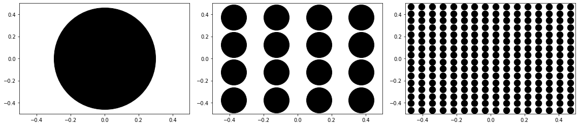
Figure 2: The homogenization process for the nuclear density $m_{N}$, illustrated at $N=1,4$ and $16$ from left to right.

We will show that this model ”converges”, in some sense that we will precise later, to the following limit model. For a 1D nuclear density $\mu$, we introduce the energy functional

$${\mathcal{E}}_{1}^{\mu}(\rho)=\int_{\mathbb{R}}\left|\nabla\sqrt{\rho}\right|^{2}+\int_{\mathbb{R}}\rho^{5/3}+\frac{1}{2}D_{1}(\rho-\mu,\rho-\mu)$$ (9)

where the 1D Hartree interaction $D_{1}$ is defined for functions decaying fast enough by

$$D_{1}(f,g)=-{2\pi}\int_{\mathbb{R}}\left(\int_{\mathbb{R}}\left|s-t\right|f(s)g(t)\mathop{}\!\mathrm{d}t\right)\mathop{}\!\mathrm{d}s$$

(more details about the 1D Hartree interaction can be read in [9]). The ground state of this model is given by the minimization problem

$$I^{\mu}_{1}=\min\{E^{\mu}(\rho),\;\rho\geqslant 0,\;\sqrt{\rho}\in X_{1},\int_{\mathbb{R}}\rho=\int_{\mathbb{R}}\mu\},$$ (10)

where

$$X_{1}=\left\{v\in H^{1}(\mathbb{R}),\;(1+\left|t\right|)^{1/2}v\in L^{2}(\mathbb{R})\right\}.$$

The following Theorem, which is a direct consequence of Theorem 1.2 and the definitions of Hartree interaction terms $D_{G}$ and $D_{1}$, is similar to [9, Theorem 2.2, Theorem 2.8], which treat Thomas-Fermi and reduced Hartree-Fock models.

Theorem 1.4.

Let $\mu\in{\mathcal{D}}({\mathbb{R}})$. Problem (10) has a unique minimizer. $u=\sqrt{\rho}$ is the unique solution of the corresponding Euler Lagrange equations

$$\begin{cases}-u^{\prime\prime}+\frac{5}{3}u^{7/3}+u\Phi=\lambda u,\\ -\Phi^{\prime\prime}=4\pi(u^{2}-\mu),\end{cases}$$

where $\lambda\in{\mathbb{R}}$, and there exists $C>0$, independent of $\mu$, such that for any $\left|t\right|\geqslant 1$, $\left|u\right|\leqslant\frac{C}{1+\left|t\right|^{3/2}}$.

Our main contribution is the following Theorem.

Theorem 1.5.

Let $m$ be a nuclear density satisfying the hypothesis of Theorem 1.2 and for $N\in{\mathbb{N}}\setminus\left\{0\right\}$, let $m_{N}$ be defined as in (8). We denote by $I_{N}=I^{m_{N}}$ and by $\rho_{N}$ the corresponding ground state given by Theorem 1.2. Let $m_{0}(t)=\frac{1}{\left|Q\right|}\int_{Q}m(\underline{x},t)\mathop{}\!\mathrm{d}\underline{x}$ and denote by $I_{0}=I^{m_{0}}_{1}$ and by $\rho_{0}$ the corresponding ground state given by Theorem 1.4. The following holds

1. $\displaystyle\lim_{N\rightarrow\infty}I_{N}=I_{0}$,

2. $\rho_{N}$ converges to $\rho_{0}$ in $L^{1}(\Gamma)$, in $L^{p}_{loc}(\Gamma)$ $\forall 1\leqslant p\leqslant 3$ and almost everywhere,

3. $\sqrt{\rho_{N}}$ converges $\sqrt{\rho_{0}}$ weakly in $H^{1}_{\rm per}(\Gamma)$.

Our result is a zero order approximation of a finite $N$ situation. In homogenization theory of partial differential equations with periodically oscillating coefficients, the two scale convergence technique is usually used to find higher order terms in the approximation [1]. Applying a similar approach to our problem is a perspective of this work.

2 Hartree interaction

We recall in this section some properties of the Green function $G$, the Hartree interaction $D_{G}$ and prove a uniqueness result on the mean-field potential $\Phi$. In the subsequent proposition, we introduce a convenient decomposition for the kernel $G$, that proves to be useful throughout the paper.

Proposition 2.1.

We have

$$G(x)=-\dfrac{2\pi}{\left|Q\right|}\left|x_{3}\right|+\dfrac{1}{\left|x\right|}+\psi(x),$$

where $\psi\in L^{\infty}(\Gamma)$.

Proposition 2.1 is partially proved in [3]. We detail the proof here for consistency.

Proof.

Using (4), we have

$$\psi(x)=-\dfrac{1}{\left|Q\right|}\int_{Q}\dfrac{\mathop{}\!\mathrm{d}\underline{y}}{\left|{x}-(\underline{y},0)\right|}+\sum_{\underline{k}\in({\mathcal{R}}^{2})^{*}}\left(\dfrac{1}{\left|{x}-(\underline{k},0)\right|}-\dfrac{1}{\left|Q\right|}\int_{Q}\dfrac{\mathop{}\!\mathrm{d}\underline{y}}{\left|{x}-(\underline{y}+\underline{k},0)\right|}\right).$$

Let us show that $\psi\in L^{\infty}(\Gamma)$. The function $\displaystyle x\mapsto\dfrac{1}{\left|Q\right|}\int_{Q}\dfrac{\mathop{}\!\mathrm{d}\underline{y}}{\left|{x}-(\underline{y},0)\right|}$ is continuous on $\Gamma$ and goes to zero as $\left|x_{3}\right|\rightarrow\infty$. Moreover, the sum defining $\psi$ converges normally on a neighborhood of $0_{{\mathbb{R}}^{3}}$ [3, Proposition 3.2]. Therefore it is continuous on that neighborhood, which implies that $\psi$ is bounded on $Q\times[-\varepsilon,\varepsilon]$, for some $\varepsilon>0$. From [3, Equation 3.12], there exists $C>0$ such that

$$\sum_{\underline{k}\in({\mathcal{R}}^{2})^{*}}\left(\dfrac{1}{\left|{x}-(\underline{k},0)\right|}-\dfrac{1}{\left|Q\right|}\int_{Q}\dfrac{\mathop{}\!\mathrm{d}\underline{y}}{\left|{x}-(\underline{y}+\underline{k},0)\right|}\right)\leqslant\dfrac{C}{\left|x_{3}\right|^{\alpha}},\quad\forall\alpha<1.$$

It follows that the $x\mapsto\sum_{\underline{k}\in({\mathcal{R}}^{2})^{*}}\left(\dfrac{1}{\left|{x}-(\underline{k},0)\right|}-\dfrac{1}{\left|Q\right|}\int_{Q}\dfrac{\mathop{}\!\mathrm{d}\underline{y}}{\left|{x}-(\underline{y}+\underline{k},0)\right|}\right)$ is bounded on $x\in Q\times({\mathbb{R}}\setminus[-\varepsilon,\varepsilon])$, thus $\psi$ is also bounded on the same interval. ∎

As a consequence of the above proposition, we prove useful properties of the potential $\Phi$. Let us introduce some notations. For some domain $\Omega\subset{\mathbb{R}}^{d}$ and $1\leqslant p\leqslant{\infty}$, we denote by

$$L^{p}_{\rm unif}(\Omega)=\left\{f\in L^{p}_{\rm loc}(\Omega),\;\forall r>0,\;\sup_{x+B_{r}\subset\Omega}\left\|f\right\|_{L^{p}(B(x,r))}<\infty\right\},$$

where $B(x,r)$ is the ball of radius $r$ centered at $x$. For $f\in L^{p}(\Gamma)$ and $g\in L^{q}(\Gamma)$, the convolution

$$(f*_{\Gamma}g)(x)=\int_{\Gamma}f(x-y)g(y)\mathop{}\!\mathrm{d}y$$

is well defined in $L^{r}(\Gamma)$, where $\frac{1}{p}+\frac{1}{q}=1+\frac{1}{r}$.

Proposition 2.2.

Let

$$Y_{{\rm per}}=\left\{f\in L^{1}(\Gamma)\cap L^{5/3}(\Gamma),\;\int_{\Gamma}f=0,\;\left|x\right|f\in L^{1}(\Gamma)\right\}.$$

The map

$$\begin{array}[]{rll}Y_{\rm per}&\to&L^{\infty}(\Gamma)\\ f&\mapsto&G*_{\Gamma}f\end{array}$$

is well defined and continuous. Moreover, for $f\in Y_{\rm per}$, $G*_{\Gamma}f$ is the unique solution, up to an additive constant, of the Poisson equation

$$\left\{\begin{array}[]{rll}\Phi&\in&L^{1}_{\text{\rm unif }}({\mathbb{R}}^{3})\\ -\Delta\Phi&=&4\pi f.\end{array}\right.$$ (11)

Proof.

From Proposition 2.1, we have that $G(x)=\frac{1}{\left|x\right|}-\dfrac{2\pi}{\left|Q\right|}\left|x_{3}\right|+\psi(x)$, with $\psi\in L^{\infty}(\Gamma)$. We are thus going to bound the three functions

$$f*_{\Gamma}\left|x_{3}\right|,\;f*_{\Gamma}\frac{1}{\left|x\right|}\;\text{and}\;f*_{\Gamma}\psi$$

in $L^{{\infty}}(\Gamma)$. First, since $\psi\in L^{\infty}(\Gamma)$, we have for any $x\in\Gamma$

$$\left|\int_{\Gamma}f(x-y)\psi(y)\mathop{}\!\mathrm{d}y\right|\leqslant\left\|\psi\right\|_{L^{\infty}(\Gamma)}\left\|f\right\|_{L^{1}(x-\Gamma)}.$$

Thus

$$\left\|f*_{\Gamma}\psi\right\|_{L^{\infty}(\Gamma)}\leqslant\left\|\psi\right\|_{L^{\infty}(\Gamma)}\left\|f\right\|_{L^{1}(\Gamma)}.$$

We move to ${f}*_{\Gamma}\frac{1}{\left|x\right|}$. We have

$$\left|f*_{\Gamma}\frac{1}{\left|x\right|}(x)\right| \leqslant\int_{\Gamma}\frac{\left|f(x-y)\right|}{\left|y\right|}\mathop{}\!\mathrm{d}y\displaystyle\leqslant\int_{\Gamma}\left|f(x-y)\right|\mathop{}\!\mathrm{d}y+\int_{\Gamma}\frac{\left|f(x-y)\right|}{\left|y\right|}\mathbbm{1}_{\left|y\right|<1}\mathop{}\!\mathrm{d}y.$$

For the second term, we use Hölder inequality with $f\in L^{5/3}(\Gamma)$ and $\frac{1}{\left|y\right|}\mathbbm{1}_{\left|y\right|<1}\in L^{5/2}(\Gamma)$. We conclude that

$$\begin{array}[]{ll}\left\|\frac{1}{\left|x\right|}*_{\Gamma}f\right\|_{L^{\infty}}&\displaystyle\leqslant\left\|f\right\|_{L^{1}(\Gamma)}+\left\|f\right\|_{L^{5/3}(\Gamma)}\left\|\frac{1}{\left|y\right|}\mathbbm{1}_{\left|y\right|<1}\right\|_{L^{5/2}(\Gamma)}.\end{array}$$

Regarding the last term, we use the neutrality assumption to write

$$\int_{\Gamma}f(x-y)\left|y_{3}\right|\mathop{}\!\mathrm{d}y=\int_{\Gamma}f(x-y)(\left|y_{3}\right|-\left|x_{3}\right|)\mathop{}\!\mathrm{d}y.$$

Thus, using the triangle inequality and the ${\mathcal{R}}$-periodicity of $x\mapsto x_{3}f(x)$, we obtain

$$\left|\int_{\Gamma}f(x-y)\left|y_{3}\right|\mathop{}\!\mathrm{d}y\right|\leqslant\int_{\Gamma}\left|f(x-y)\right|\left|x_{3}-y_{3}\right|\mathop{}\!\mathrm{d}y=\int_{\Gamma}\left|f(y)\right|\left|y_{3}\right|\mathop{}\!\mathrm{d}y.$$

Finally, we need to prove that $\Phi-G*_{\Gamma}f$ is constant for any solution $\Phi$ of (11). Notice first that $h=\Phi-G*_{\Gamma}f$ is a harmonic function over $\mathbb{R}^{3}$. By the mean value Theorem for a harmonic functions, we have that

$$\left(\Phi-h\right)(x)=\int_{B(x,1)}\left(\Phi-h\right)(y)\mathop{}\!\mathrm{d}y\leqslant\sup_{x\in\Gamma}\int_{B(x,1)}\left(\Phi-h\right)(y)\mathop{}\!\mathrm{d}y\leqslant\left\|\Phi-h\right\|_{L^{1}_{unif}}.$$

Therefore, $\Phi-h$ is harmonic and bounded in $\Gamma.$ By Louisville’s Theorem, we conclude that $\Phi-h$ is constant. ∎

Corollary 2.3.

Let $f\in Y_{per}$, then $\nabla(G*_{\Gamma}f)\in\left(L^{2}(\Gamma)\right)^{3}$ and there exists $C>0$, such that

$$D_{G}(f,f)=\left\|\nabla(G*_{\Gamma}f)\right\|^{2}_{L^{2}(\Gamma)}\leqslant C\left\|f\right\|_{L^{1}(\Gamma)}\left(\left\|f\right\|_{L^{1}(\Gamma)}+\left\|f\right\|_{L^{5/3}(\Gamma)}+\left\||x_{3}|f\right\|_{L^{1}(\Gamma)}\right).$$

Proof.

We have

$$D_{G}(f,f)=\int_{\Gamma}(G*_{\Gamma}f)\times f=\int_{\Gamma}(G*_{\Gamma}f)\times\Delta(G*_{\Gamma}f)=\int_{\Gamma}\left|\nabla(G*_{\Gamma}f)\right|^{2}.$$

Besides, by the previous proposition $G*_{\Gamma}f\in L^{\infty}(\Gamma)$ and

$$\left\|G*_{\Gamma}f\right\|_{L^{\infty}(\Gamma)}\leqslant(\left\|\psi\right\|_{L^{\infty}(\Gamma)}+1)\left\|f\right\|_{L^{1}(\Gamma)}+\left\|f\right\|_{L^{5/3}(\Gamma)}\left\|\frac{1}{\left|y\right|}\mathbbm{1}_{\left|y\right|<1}\right\|_{L^{5/2}(\Gamma)}+\left\|\left|x\right|f\right\|_{L^{1}(\Gamma)}\leqslant C\left\|f\right\|_{Y_{{\rm per}}},$$

which proves the inequality stated in the corollary.

∎

3 Homogenization procedure: proof of Theorem 1.5

This section is devoted to the proof of Theorem 1.5. The strategy of the proof is as follows. We start by proving the convergence of the nuclear densities $(m_{N})$. Indeed, when $N$ increases, the nuclear density $m_{N}$ becomes more homogeneous and the sequence $(m_{N})$ converges to the 2D homogeneous density $m_{0}(x_{3})=\frac{1}{\left|Q\right|}\int_{Q}m(x)\mathop{}\!\mathrm{d}\underline{x}$ (see Lemma 3.3). The electronic densities $\rho_{N}$ are uniformly bounded with respect to $N$. We can thus extract convergent subsequences (see Proposition 3.5). Both convergences give the upper bound $I\leqslant\liminf I_{N}$. To prove the lower bound $I_{0}\geqslant\limsup I_{N}$, we use $\rho_{0}$ as a test function. The proof is divided into four steps.

Step 1: Properties of the sequence $(m_{N})$

We state in this section two properties of the sequence $(m_{N})$.

Lemma 3.1.

For $p\geqslant 1$ and $f\in L^{1}_{\rm loc}({\mathbb{R}})$ such that $x\mapsto f(x_{3})m^{p}(x)\in L^{1}(\Gamma)$, we have

$$\int_{Q}m_{N}^{p}(\underline{x},x_{3})\mathop{}\!\mathrm{d}\underline{x}=\int_{Q}m^{p}(\underline{x},x_{3})\mathop{}\!\mathrm{d}\underline{x},$$

and

$$\int_{\Gamma}f(x_{3})m_{N}^{p}(x)\mathop{}\!\mathrm{d}x=\int_{\Gamma}f(x_{3})m^{p}(x)\mathop{}\!\mathrm{d}x.$$

Proof.

We have

$$\int_{Q}m_{N}^{p}(x_{1},x_{2},x_{3})\mathop{}\!\mathrm{d}x_{1}\mathop{}\!\mathrm{d}x_{2}=\int_{Q}m^{p}(Nx_{1},Nx_{2},x_{3})\mathop{}\!\mathrm{d}x_{1}\mathop{}\!\mathrm{d}x_{2}=\frac{1}{N^{2}}\int_{NQ}m^{p}(y_{1},y_{2},x_{3})\mathop{}\!\mathrm{d}y_{1}\mathop{}\!\mathrm{d}y_{2}.$$

As $m$ is $Q$-periodic then, $\displaystyle\int_{NQ}m^{p}(y_{1},y_{2},x_{3})\mathop{}\!\mathrm{d}y_{1}\mathop{}\!\mathrm{d}y_{2}=N^{2}\int_{Q}m^{p}(y_{1},y_{2},x_{3})\mathop{}\!\mathrm{d}y_{1}\mathop{}\!\mathrm{d}y_{2}$. Hence, the first claim is proved. The second claim easily follows. ∎

Remark 3.2.

By the second point of Lemma 3.1, we have that $\int_{\Gamma}m_{N}=\int_{\Gamma}m=\int_{\Gamma}m_{0}$, so that any admissible state for $I_{N}$ is also an admissible state for $I_{0}$, and vice versa.

Lemma 3.3.

The sequence $(m_{N})$ converges to $m_{0}$ weakly in $L^{p}(\Gamma)$ $\forall 1\leqslant p<+{\infty}$.

Proof.

From the $Q$-periodicity of $m$, we have for any $x_{3}\in{\mathbb{R}}$ (see for instance [13])

$$m_{N}(\cdot,\cdot,x_{3})\rightharpoonup m_{0}(\cdot,\cdot,x_{3})\quad\mbox{ in }L^{p}(Q)\quad\forall 1\leqslant p<{\infty}.$$ (12)

For $\varphi\in L^{q}(Q)$ and $\psi\in L^{q}({\mathbb{R}})$, with $\frac{1}{q}+\frac{1}{p}=1$, we have $f_{N}(x_{3}):=\displaystyle\int_{Q}m_{N}(x)\varphi(\underline{x})\psi(x_{3})\mathop{}\!\mathrm{d}\underline{x}\to f(x_{3}):=m_{0}(x_{3})\psi(x_{3})\int_{Q}\varphi(\underline{x})\mathop{}\!\mathrm{d}\underline{x}$ a.e. and

$$\left|f_{N}(x_{3})\right| \leqslant\left\|\varphi\right\|_{L^{q}(Q)}\left|\psi(x_{3})\right|\left(\int_{Q}\left|m_{N}(\underline{x},x_{3})\right|^{p}\mathop{}\!\mathrm{d}\underline{x}\right)^{1/p}=\left\|\varphi\right\|_{L^{q}(Q)}\left|\psi(x_{3})\right|\left(\int_{Q}\left|m(\underline{x},x_{3})\right|^{p}\mathop{}\!\mathrm{d}\underline{x}\right)^{1/p}.$$ (13)

Thus, by dominated convergence Theorem,

$$\int_{\mathbb{R}}f_{N}(x_{3})\mathop{}\!\mathrm{d}x_{3}=\int_{\Gamma}m_{N}(x)\varphi(\underline{x})\psi(x_{3})\mathop{}\!\mathrm{d}x\to\int_{\mathbb{R}}f(x_{3})\mathop{}\!\mathrm{d}x_{3}=\int_{\Gamma}m_{0}(x_{3})\varphi(\underline{x})\psi(x_{3})\mathop{}\!\mathrm{d}x.$$

By the density of $L^{q}(Q)\otimes L^{q}({\mathbb{R}})$ in $L^{q}(\Gamma)$, the proof is complete. ∎

Step 2: Convergence of electronic densities

The following proposition gives uniform bounds on quantities of interest with respect to $N$.

Proposition 3.4.

There exist various constants $C$ independent of $N$ such that the following bounds hold.

1. $\displaystyle I_{N}\leqslant C$,

2. $\displaystyle\left\|\sqrt{\rho_{N}}\right\|_{H^{1}(\Gamma)}\leqslant C$,

3. $\displaystyle\left\|\rho_{N}\right\|_{L^{p}({\Gamma})}\leqslant C$ for all $1\leqslant p\leqslant 3$,

4. $\displaystyle D_{G}(\rho_{N}-m_{N},\rho_{N}-m_{N})\leqslant C$,

Proof.

As $\rho_{N}$ is the minimizer of $I_{N}$ and since $m$ is an admissible test function for ${\mathcal{E}}^{m_{N}}_{\rm per}$, we have

$$I_{N}={\mathcal{E}}_{per}^{m_{N}}(\rho_{N})\leqslant{\mathcal{E}}_{per}^{m_{N}}(m)=\int_{\Gamma}\left|\nabla\sqrt{m}\right|^{2}+\int_{\Gamma}m^{5/3}+\frac{1}{2}D_{G}(m-m_{N},m-m_{N}).$$

By corollary 2.3 applied to $f=m-m_{N}$ and Lemma 3.1, we have

$$\begin{array}[]{lll}D_{G}(m-m_{N},m-m_{N})&\leqslant&C\left\|m-m_{N}\right\|_{L^{1}(\Gamma)}\left(\left\|m-m_{N}\right\|_{L^{1}(\Gamma)}+\left\|m-m_{N}\right\|_{L^{5/3}(\Gamma)}\right.\\ &&\left.+\left\||x_{3}|(m-m_{N})\right\|_{L^{1}(\Gamma)}\right)\\ &\leqslant&C\left\|m\right\|_{L^{1}(\Gamma)}\left(\left\|m\right\|_{L^{1}(\Gamma)}+\left\|m\right\|_{L^{5/3}(\Gamma)}+\left\||x_{3}|m\right\|_{L^{1}(\Gamma)}\right).\end{array}$$

Points II-IV are easily deduces from point point I. ∎

Proposition 3.5.

There exists a non negative function $\rho_{0}\in L^{1}(\Gamma)\cap L^{5/3}(\Gamma)$ such that, up to a subsequence,

• $(\rho_{N})$ converges to $\rho_{0}$ strongly in $L^{1}(\Gamma)$ and $L^{p}_{loc}(\Gamma)$ for all $1\leqslant p\leqslant 3$, weakly in $L^{p}(\Gamma)$ and almost everywhere on $\mathbb{R}^{3}$,

• $(\nabla\sqrt{\rho_{N}})$ converges to $\nabla\sqrt{\rho_{0}}$ weakly in $(L^{2}(\Gamma))^{3}$

• $\rho_{0}-m_{0}\in Y_{\rm per}$

• The sequence $\nabla\Phi_{N}=\nabla\left(G*_{\Gamma}(\rho_{N}-m_{N})\right)$ converges to $\nabla\Phi_{0}=\nabla\left(G*_{\Gamma}(\rho_{0}-m_{0})\right)$ weakly in $(L^{2}(\Gamma))^{3}$.

As a consequence

$${\mathcal{E}}_{\rm per}^{m_{0}}(\rho_{0})\leqslant\liminf I_{N}.$$

Proof.

The sequence $(\sqrt{\rho_{N}})_{N}$ is uniformly bounded with respect to $N$ in $H^{1}(\Gamma)$ by Proposition 3.4. Then, up to a subsequence, it converges to some non negative function $u_{0}$ weakly in $H^{1}(\Gamma)$, strongly in $L^{p}_{loc}(\Gamma)$ for all $2\leqslant p\leqslant 6$ and almost everywhere on $\mathbb{R}^{3}$. Besides, by Theorem 1.2, there exists $C\geqslant 0$ such that for any $N$ and any $x\in{\mathbb{R}}^{3}$ such that $\left|x_{3}\right|\geqslant 1$, it holds

$$\left|u_{N}(x)\right|\leqslant\frac{C}{1+\left|x_{3}\right|^{3/2}}.$$

By the almost everywhere convergence, $u_{0}$ satisfies the same estimate, and we have for $\rho_{0}:=u_{0}^{2}$ the following estimate

$$\left|x_{3}\right|\rho_{0}(x)\leqslant\rho_{0}(x)1_{\left|x_{3}\right|\leqslant 1}+\frac{C}{1+\left|x_{3}\right|^{3}}\in L^{1}(\Gamma).$$

Thus $\rho_{0}\in L^{1}(\Gamma)\cap L^{5/3}(\Gamma)$ and $\left|x_{3}\right|\rho_{0}\in L^{1}(\Gamma)$.

We show now that $\rho_{N}$ converges to $\rho_{0}$ strongly in $L^{1}(\Gamma)$. Let $\varepsilon>0$ and $R$ large enough such that for any $M,N\in{\mathbb{N}}\setminus\{0\}$

$$\int_{\left|x_{3}\right|>R}\left|\rho_{N}-\rho_{M}\right|\leqslant\frac{1}{R}\int_{\left|x_{3}\right|>R}\left|x_{3}\right|\left|\rho_{N}-\rho_{M}\right|\leqslant\frac{C}{R}\leqslant\frac{\varepsilon}{2}.$$

By the strong convergence of $\rho_{N}$ in $L^{1}_{\rm loc}(\Gamma)$, for $M,N$ large enough, we have

$$\int_{\left|x_{3}\right|<R}\left|\rho_{N}-\rho_{M}\right|\leqslant\frac{\varepsilon}{2},$$

which proves that $(\rho_{N})$ is a Cauchy sequence. Besides, $(\nabla\Phi_{N})$ is uniformly bounded in $L^{2}(\Gamma)$. Thus, it weakly converges, up to a subsequence, to $W\in\left(L^{2}(\Gamma)\right)^{3}$. Since $-\Delta\Phi_{N}=4\pi\left(\rho_{N}-m_{N}\right)$, then, $\forall\varphi\in{\mathcal{D}}(\Gamma)$, we have

$$\int_{\Gamma}\nabla\Phi_{N}\nabla\varphi=4\pi\int_{\Gamma}\left(\rho_{N}-m_{N}\right)\varphi.$$ (14)

By definition of the weak limit, the LHS of (14) converges to $\int_{\Gamma}W\nabla\varphi$, and since $\rho_{N}-m_{N}$ weakly converges to $\rho_{0}-m_{0}$ in $L^{1}(\Gamma)$, then

$$\forall\varphi\in{\mathcal{D}}(\Gamma)\quad\int_{\Gamma}W\nabla\varphi=4\pi\int_{\Gamma}\left(\rho_{0}-m_{0}\right)\varphi.$$

Therefore ${\rm div\;}W=4\pi(\rho_{0}-m_{0})$. By taking the mixed Fourier transform defined in [3, Eq. 3.13] , we get for $\underline{R}$ in the dual lattice ${\mathcal{R}}^{*}$ and $\eta\in{\mathbb{R}}$

$$2i\pi\left(\begin{array}[]{c}R_{1}\\ R_{2}\\ \eta\end{array}\right)\cdot\widehat{W}(R,\eta)=(\widehat{\rho_{0}-m_{0}})(R,\eta).$$

For $\underline{R}=0$ and $\eta=0$, we obtain $\displaystyle\int_{\Gamma}\rho_{0}-m_{0}=0$. It follows that $\rho_{0}-m_{0}\in Y_{\rm per}$. Thus by Proposition 2.2, $\Phi_{0}:=G*_{\Gamma}(\rho_{0}-m_{0})$ is well defined. Finally, we show that $\nabla\Phi_{0}=W$. Let $\varphi=(\varphi_{1},\varphi_{2},\varphi_{3})\in{\mathcal{D}}(\Gamma)^{3}$. We have ${\rm div\;}\varphi\in Y_{\rm per}$, thus $G*_{\Gamma}({\rm div\;}\varphi)\in L^{\infty}(\Gamma)$. Therefore

$$\langle\nabla G*_{\Gamma}(\rho_{N}-m_{N}),\varphi\rangle =\langle\rho_{N}-m_{N},G*_{\Gamma}{\rm div\;}\varphi\rangle$$

$$\to\langle\rho_{0}-m_{0},G*_{\Gamma}{\rm div\;}\varphi\rangle=\langle\nabla G*_{\Gamma}(\rho_{0}-m_{0}),\varphi\rangle.$$

∎

Step 3: Identification of the limit

We show in this section that $\rho_{0}$ is invariant with respect to $(x_{1},x_{2})$ and it is indeed the unique minimizer of ${\mathcal{E}}_{1}^{m_{0}}$. This will prove that the convergences in Proposition 3.5 hold for the whole sequence and prove points ii-iii of Theorem 1.5.

We start by showing that $\rho_{0}$ is the unique minimizer of ${\mathcal{E}}^{m_{0}}_{\rm per}$.

Proposition 3.6.

$\rho_{0}$ is the unique minimizer of ${\mathcal{E}}^{m_{0}}_{\rm per}$.

Proof.

Let $\rho\in\left\{\rho\geqslant 0,\;\sqrt{\rho}\in X_{\rm per},\;\int_{\Gamma}\rho=\int_{\Gamma}m_{0}\right\}$ an admissible test function for ${\mathcal{E}}^{m_{0}}_{\rm per}$. Let us show that

$${\mathcal{E}}_{\rm per}^{m_{0}}(\rho_{0})\leqslant{\mathcal{E}}_{\rm per}^{m_{0}}(\rho).$$

As $\int_{\Gamma}m_{0}=\int_{\Gamma}m_{N}$, $\rho$ is also an admissible test function for ${\mathcal{E}}_{\rm per}^{m_{N}}$. Thus

$$I_{N}={\mathcal{E}}_{\rm per}^{m_{N}}(\rho_{N})\leqslant{\mathcal{E}}_{\rm per}^{m_{N}}(\rho).$$

We know from Proposition 3.5 that

$${\mathcal{E}}^{m_{0}}_{\rm per}(\rho_{0})\leqslant\liminf I_{N}\leqslant\liminf{\mathcal{E}}_{\rm per}^{m_{N}}(\rho).$$

It thus remains to show that ${\mathcal{E}}_{\rm per}^{m_{N}}(\rho)\to{\mathcal{E}}_{\rm per}^{m_{0}}(\rho)$, which boils down to showing that

$$D_{G}(\rho-m_{N},\rho-m_{N})\to D_{G}(\rho-m_{0},\rho-m_{0}).$$ (15)

We recall that

$$D_{G}(f,g)=\int_{\Gamma\times\Gamma}f(x)f(y)G(x-y)\mathop{}\!\mathrm{d}x\mathop{}\!\mathrm{d}y,$$

with $G(x)=-2\pi\left|x_{3}\right|+\frac{1}{\left|x\right|}+\psi(x)$, $\psi\in L^{\infty}(\Gamma)$. We denote by $h_{N}=\rho-m_{N}$ and $h=\rho-m_{0}$. We recall as well that for any $x_{3}\in{\mathbb{R}}$ $h_{N}(\cdot,x_{3})$ converges to $h(\cdot,x_{3})$ weakly in $L^{p}(Q)$, $\forall 1\leqslant p<{\infty}$. Therefore, for any $x_{3},y_{3}\in{\mathbb{R}}$, $h_{N}(\cdot,x_{3})h_{N}(\cdot,y_{3})$ converges to $h(\cdot,x_{3})h(\cdot,y_{3})$ weakly in $L^{p}(Q\times Q)$. We have $-2\pi\left|x_{3}-y_{3}\right|+\psi(x-y)\in L^{\infty}(Q\times Q)$, and $\frac{1}{\left|x-y\right|}\in L^{p}(Q\times Q)$ for any $1\leqslant p<2$. Therefore, for any $x_{3},y_{3}\in{\mathbb{R}}$

$$\int_{Q\times Q}h_{N}(x)h_{N}(y)G(x-y)\mathop{}\!\mathrm{d}\underline{x}\mathop{}\!\mathrm{d}\underline{y}\to\int_{Q\times Q}h(x)h(y)G(x-y)\mathop{}\!\mathrm{d}\underline{x}\mathop{}\!\mathrm{d}\underline{y}.$$ (16)

To use a dominated convergence argument, we need to bound the LHS of (16) uniformly with respect to $N$ by an $L^{1}$ function with respect to $(x_{3},y_{3})$. We start with the term with $\psi$. We have

$$\left|\int_{Q\times Q}h_{N}(x)h_{N}(y)\psi(x-y)\mathop{}\!\mathrm{d}\underline{x}\mathop{}\!\mathrm{d}\underline{y}\right|\leqslant\left\|\psi\right\|_{L^{\infty}(\Gamma)}\int_{Q}\left|h_{N}(x)\right|\mathop{}\!\mathrm{d}\underline{x}\int_{Q}\left|h_{N}(y)\right|\mathop{}\!\mathrm{d}\underline{y},$$

where

$$\int_{Q}\left|h_{N}\right|\mathop{}\!\mathrm{d}\underline{x}\leqslant\int_{Q}{\rho}\mathop{}\!\mathrm{d}\underline{x}+\int_{Q}{m_{N}}\mathop{}\!\mathrm{d}\underline{x}=\int_{Q}\rho\mathop{}\!\mathrm{d}\underline{x}+\int_{Q}{m}\mathop{}\!\mathrm{d}\underline{x}.$$ (17)

The RHS of (17) is indeed an $L^{1}$ function wrt to $x_{3}$ and $y_{3}$. We move to the term with $\left|x_{3}\right|$. We have

$$\left|\int_{Q\times Q}h_{N}(x)h_{N}(y)\left|x_{3}-y_{3}\right|\mathop{}\!\mathrm{d}\underline{x}\mathop{}\!\mathrm{d}\underline{y}\right| \leqslant\int_{Q}\left|x_{3}\,h_{N}(x)\right|\mathop{}\!\mathrm{d}\underline{x}\int_{Q}\left|h_{N}(y)\right|\mathop{}\!\mathrm{d}\underline{y}+\int_{Q}\left|y_{3}\,h_{N}(y)\right|\mathop{}\!\mathrm{d}\underline{y}\int_{Q}\left|h_{N}(x)\right|\mathop{}\!\mathrm{d}\underline{x}$$

$$\leqslant\left(\int_{Q}\left|x_{3}\right|\left(\rho(x)+m(x)\right)\mathop{}\!\mathrm{d}\underline{x}\right)\left(\int_{Q}\left(\rho(y)+m(y)\right)\mathop{}\!\mathrm{d}\underline{y}\right)$$

$$\quad+\left(\int_{Q}\left|y_{3}\right|\left(\rho(y)+m(y)\right)\mathop{}\!\mathrm{d}\underline{y}\right)\left(\int_{Q}\left(\rho(x)+m(x)\right)\mathop{}\!\mathrm{d}\underline{x}\right).$$ (18)

Again, the RHS of (3) is an $L^{1}$ function wrt $x_{3}$ and $y_{3}$. Finally, for the term with $\frac{1}{\left|x\right|}$, we split the term as follows

$$\int_{Q\times Q}h_{N}(x)h_{N}(y)\frac{1}{\left|x-y\right|}\mathop{}\!\mathrm{d}\underline{x}\mathop{}\!\mathrm{d}\underline{y} =\int_{Q\times Q}\rho(x)\left(\rho(y)-2m_{N}(y)\right)\frac{1}{\left|x-y\right|}\mathop{}\!\mathrm{d}\underline{x}\mathop{}\!\mathrm{d}\underline{y}$$

$$+\int_{Q\times Q}m_{N}(x)m_{N}(y)\frac{1}{\left|x-y\right|}\mathop{}\!\mathrm{d}\underline{x}\mathop{}\!\mathrm{d}\underline{y}.$$

The first term is bounded by

$$\left|\int_{Q\times Q}\rho(x)\left(\rho(y)-2m_{N}(y)\right)\frac{1}{\left|x-y\right|}\mathop{}\!\mathrm{d}\underline{x}\mathop{}\!\mathrm{d}\underline{y}\right| \leqslant\left\|\rho*\frac{1}{\left|x\right|}\right\|_{L^{\infty}(\Gamma)}\left\|\rho+2m(\cdot,x_{3})\right\|_{L^{1}(Q)}$$

which is an $L^{1}$ function with respect to $x_{3}$. For the second term we use Young inequality with $p=q=r=3/2$. We obtain

$$\left|\int_{Q\times Q}m_{N}(x)m_{N}(y)\frac{1}{\left|x-y\right|}\mathop{}\!\mathrm{d}\underline{x}\mathop{}\!\mathrm{d}\underline{y}\right| \leqslant\left\|m_{N}(\cdot,x_{3})\right\|_{L^{3/2}(Q)}\left\|m_{N}(\cdot,y_{3})\right\|_{L^{3/2}(Q)}\left\|\frac{1}{\left|x\right|}\right\|_{L^{3/2}(Q)}$$

$$\leqslant\left\|m(\cdot,x_{3})\right\|_{L^{3/2}(Q)}\left\|m(\cdot,y_{3})\right\|_{L^{3/2}(Q)}\times\left\|\frac{1}{\left|\underline{x}\right|}\right\|_{L^{3/2}(Q)}.$$ (19)

As $m$ is compactly supported in $x_{3}$, $x_{3}\mapsto\left\|m(\cdot,x_{3})\right\|_{L^{3/2}(Q)}$ is also compactly supported and it is an $L^{3/2}$ function, thus, it is an $L^{1}$; which concludes the proof. ∎

Proposition 3.7.

The density $\rho_{0}$ is invariant wrt $(x_{1},x_{2})$, it is indeed the unique minimizer of the 1D model ${\mathcal{E}}_{1}^{m_{0}}$ and

$$I_{0}={\mathcal{E}}_{\rm per}^{m_{0}}(\rho_{0})={\mathcal{E}}_{1}^{m_{0}}(\rho_{0}).$$

Proof.

For any $\underline{R}\in{\mathbb{R}}^{2}$, $\tau_{\underline{R}}\rho_{0}$ is also a minimizer of ${\mathcal{E}}_{\rm per}^{m_{0}}$, where $\tau$ is the translation operator. Thus, by the convexity of the functional ${\mathcal{E}}_{\rm per}^{m_{0}}$ and the uniqueness of its minimizer (see Theorem 1.2), we deduce that $\rho_{0}$ is invariant with respect to $(x_{1},x_{2})$. To conclude the proof of the proposition, we notice that for any ${\mathbb{R}}^{2}$-invariant function $f$

$$D_{G}(f,f)=D_{1}(f,f),$$

as shown in [9, Propo. 3.1].

∎

Step 4: Convergence of the energy

We prove in this section point i of Theorem 1.5, which consists of the convergence of the energy.

Proposition 3.8.

We have

$$I_{0}=\lim I_{N}.$$

Proof.

By Propositions 3.5 and 3.7, we have

$$I_{0}\leqslant\liminf I_{N}.$$

To prove the lower bound on $I_{0}$, we use $\rho_{0}$ as a test function for ${\mathcal{E}}_{\rm per}^{m_{N}}$ and obtain

$$\begin{split}I_{N}\leqslant\int_{\Gamma}\left|\nabla\sqrt{\rho_{0}}\right|^{2}+\int_{\Gamma}\rho_{0}^{5/3}+D_{G}(\rho_{0}-m_{N},\rho_{0}-m_{N})\to{\mathcal{E}}_{\rm per}^{m_{0}}(\rho_{0})=I_{0},\end{split}$$

where the last convergence is obtained using (15). Thus

$$\limsup I_{N}\leqslant I_{0},$$

which concludes the proof of the proposition.

∎

4 Numerical illustration

In this section, we illustrate the convergence result of Theorem 1.5. We recall that the minimization problem (6) has a unique minimizer $\rho$, and $u=\sqrt{\rho}$ is the unique solution of the corresponding Euler-Lagrange equations

$$\left\{\begin{array}[]{rll}\Delta u+\frac{5}{3}u^{\frac{7}{3}}+u\Phi&=&-\lambda u,\\ -\Delta\Phi&=&4\pi(u^{2}-\mu).\end{array}\right.$$ (20)

We solve the 3D periodic Euler-Lagrange system in (20) by coupling a spectral approach and a fixed point iterative scheme. We adopt the following iterative fixed point scheme : starting form an arbitrary initial guess $u_{0}$, at each fixed point iteration, a linear eigenvalue problem is solved

$$\left(\Delta+\frac{5}{3}u_{n}^{4/3}+\Phi_{n}\right)u_{n+1}=-\lambda_{1}u_{n+1},$$ (21)

with $\Phi_{n}$ the solution to the Poisson equation $-\Delta\Phi_{n}=4\pi(u_{n}^{2}-\mu)$. The fixed point iterations are continued until convergence, i.e. $\left\|u_{n}-u_{n+1}\right\|_{2}\leqslant\varepsilon$ for some tolerance $\varepsilon>0$. We take $\varepsilon=10^{-6}$ in our simulations.

We adopt a periodic setting, with the unit cell $\textstyle\Gamma=Q\times[-\frac{L}{2},\frac{L}{2}]$, with $Q=\left[-\frac{1}{2},\frac{1}{2}\right]^{2}$. We use a Fourier series decomposition approach to solve the linearized equation (21). The solution is expected to be ${\mathcal{R}}-$periodic with respect to $x_{1}$ and $x_{2}$ and decaying at infinity with respect to $|x_{3}|$. Taking a large value for $L$, it is reasonable to impose period conditions in the third direction as well. Therefore, we consider the Fourier basis

$$f_{k}(x)=\frac{1}{\sqrt{L}}e^{i2\pi\left(\underline{x}\cdot\underline{k}+\frac{k_{3}x_{3}}{L}\right)}.$$

We illustrate the convergence results in Theorem 1.5 using the series of nuclei densities $m_{N}$ defined as

$$m_{N}(x_{1},x_{2},x_{3})=\mu(N\cdot\,x_{1})m_{0}(x_{3})=\frac{\pi}{2}\left|\cos(N\pi x_{1})\right|\times 5\exp\left(-\frac{x_{3}^{2}}{8}\right).$$

We note that $\int_{Q}\mu(N\cdot x_{1})\,\rm{d}x_{1}\,\rm{d}x_{2}=\frac{\pi}{2}\int_{Q}\left|\cos(N\cdot\pi x_{1})\right|=1$. We take $L=2\pi$, which proves effective as the function $m_{0}(x_{3})=5\exp\left(-\frac{x_{3}^{2}}{8}\right)$ rapidly decreases in the $x_{3}$ direction. The same behaviour is assumed for the solutions $u_{N}$, and is validated with 1D simulations for $(u_{0},\rho_{0})$, the 1D solution corresponding to $m_{0}$.

The different functions are sampled on a grid of dimensions $(200\times N,4,300)$. We keep the discretization constant along the $y$ and $z$-axis as the homogenization is only applied in the $x_{3}$ dimension. As we will only compute the zero Fourier mode along $x_{2}$, four points are largely enough. We compute the positive Fourier modes up to indices $K=(K_{1},K_{2},K_{3})=(4\times N,0,6)$. On the $x_{3}$-axis, we use the first $7$ Fourier modes, found to be sufficient for accurate reconstruction of $m_{N}$ and $m_{0}$ along that axis. Simulations in 1D prove that the solution $(u_{0}(x_{3}),\rho_{0}(x_{3}))$, is also accurately represented by these $7$ modes. We assume that this is also the case in 3D for all values of $N$. The choice of $(4N+1)$ Fourier modes in the $x_{1}$ direction, is motivated by the need for increased Fourier modes as $N$ grows, to capture the changing characteristics and new harmonics for $m_{N}$ and ’eventually’ for the solution $(\rho_{N},u_{N})$. In fact, we know that $(\rho_{N},u_{N})$ will rather converge to a constant along the axis $x_{1}$ by Theorem 1.5, however we enforce a hard check for this by computing also large modes for $\rho_{N}$ and $u_{N}$ .

Different $L^{p}$-norms of the error $e_{N}=\rho_{N}-\rho_{0}$ are presented in Figure 3 for values of $N=1,\ldots,5$. We, indeed, observe the convergence stated in Theorem 1.5. The same figure shows some convergence rates estimates. We conjecture that we have a theoretical convergence rate of $1/N^{r}$ with $\frac{10}{3}<r<4$ for the different norms of $e_{n}$ and the gradient $L^{2}$ norm $\left\|\nabla{u_{n}}-\nabla{u_{0}}\right\|_{2}$. The discrepancies in Figure 3 at $N=4,5$ are probably due to numerical errors.

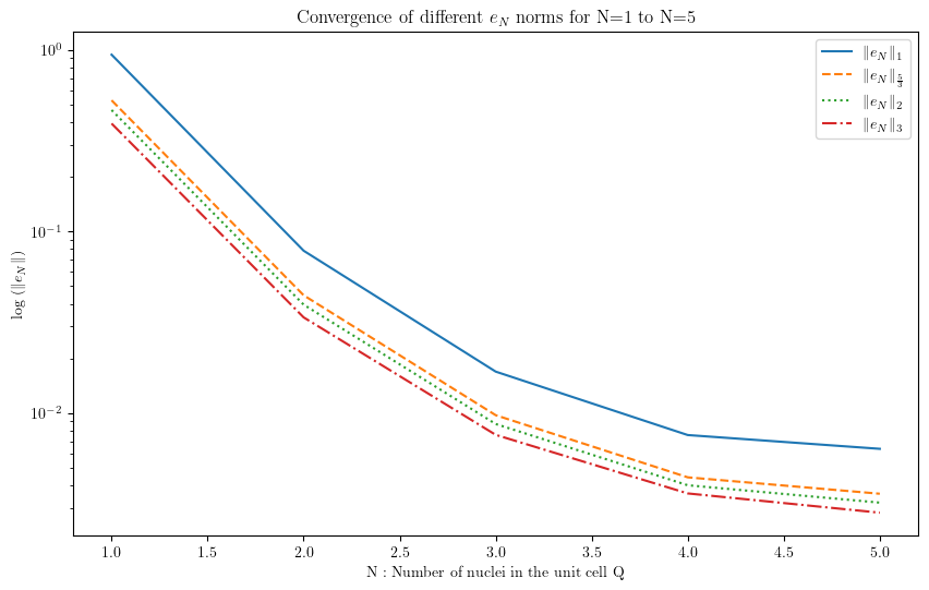
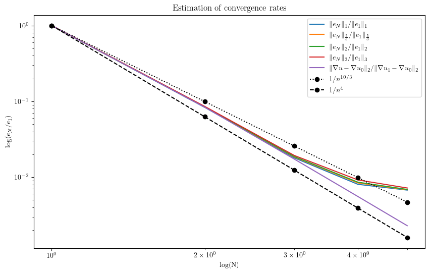
Figure 3: Convergence analysis for $e_{n}$ norms (left) and convergence rates estimation for $e_{n}$ norms and the gradient $L^{2}$ norm $\left\|\nabla{u_{n}}-\nabla{u_{0}}\right\|_{2}$ (right).

Figure 4 illustrates the convergence of the ground state energy $I_{N}={\mathcal{E}}^{m_{N}}_{per}(\rho_{N})$ to the 1D energy $I_{0}={\mathcal{E}}^{m_{0}}_{1}(\rho_{0})$, proved in Theorem 1.5. The estimated convergence rate for the energy is of the order $\approx\dfrac{1}{N^{3/2}}$.

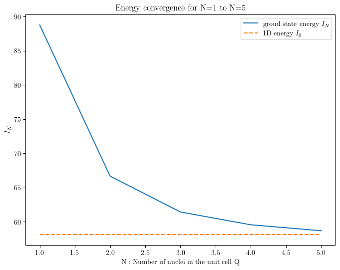
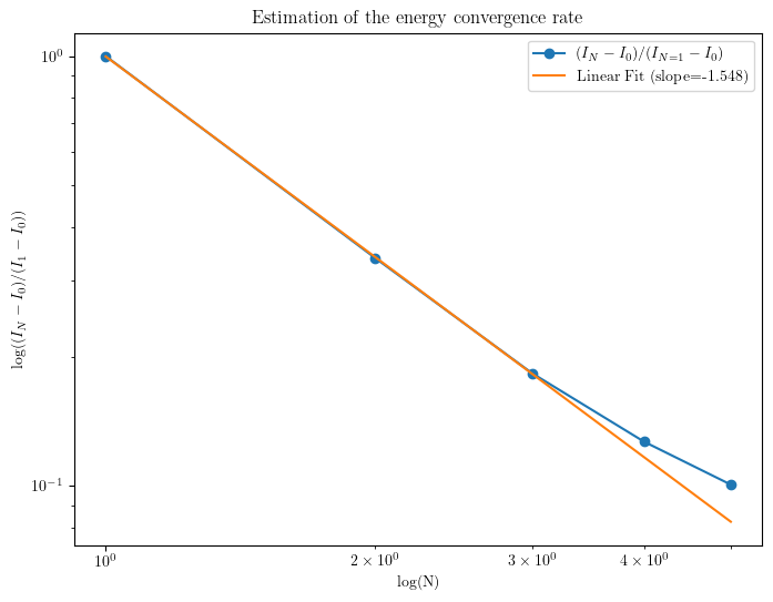
Figure 4: Convergence analysis for the energies $I_{N}$ (left) and convergence rate estimation (right).

Remark 4.1.

It is noteworthy to mention that, for $N\geqslant 6$, and using higher order Fourier modes, the presence of numerical errors hinders a clear observation of further convergence for $e_{N}$.

References

• [1] G. Allaire, Homogenization and two-scale convergence, SIAM Journal on Mathematical Analysis, 23 (1992), pp. 1482–1518.
• [2] R. Benguria, H. Brezis, and E. Lieb, The Thomas-Fermi-von weizsäcker theory of atoms and molecules, Communications in Mathematical Physics, 79 (1981), pp. 167–180.
• [3] X. Blanc and C. Le Bris, Thomas-fermi type theories for polymers and thin films, Advances in Differential Equations, 5 (2000), pp. 977–1032.
• [4] X. Blanc and R. Monneau, Screening of an applied electric field inside a metallic layer described by the Thomas-Fermi-von Weizsäcker model, Advances in Differential Equations, 7 (2002), pp. 847 – 876.
• [5] A. Carvalho, P. E. Trevisanutto, S. Taioli, and A. H. C. Neto, Computational methods for 2d materials modelling, Reports on Progress in Physics, 84 (2021), p. 106501.
• [6] I. Catto, C. Le Bris, and P. L. Lions, Mathematical theory of thermodynamic limits : Thomas- Fermi type models, Oxford University Press, 1998.
• [7] V. Chaudhary, P. Neugebauer, O. Mounkachi, S. Lahbabi, and A. E. Fatimy, Phosphorene—an emerging two-dimensional material: recent advances in synthesis, functionalization, and applications, 2D Materials, 9 (2022), p. 032001.
• [8] A. Geim and I. Grigorieva, Van der Waals heterostructures, Nature, 499 (2013), pp. 419–425.
• [9] D. Gontier, S. Lahbabi, and A. Maichine, Density functional theory for two-dimensional homogeneous materials, Communications in Mathematical Physics, 388 (2021), pp. 1475–1505.
• [10] D. Gupta, V. Chauhan, and R. Kumar, A comprehensive review on synthesis and applications of molybdenum disulfide MoS2 material: Past and recent developments, Inorganic Chemistry Communications, 121 (2020), p. 108200.
• [11] F. Hussain, M. Imran, and H. Ullah, Density Functional Theory (DFT) Study of Novel 2D and 3D Materials, Springer Singapore, Singapore, 2017, pp. 269–284.
• [12] E. H. Lieb and B. Simon, The Thomas-Fermi theory of atoms, molecules and solids, Advances in Mathematics, 23 (1977), pp. 22–116.
• [13] D. Lukkassen and P. Wall, On weak convergence of locally periodic functions, Journal of Nonlinear Mathematical Physics, 9 (2002), pp. 42–57.
• [14] A. Patra, S. Jana, P. Samal, F. Tran, L. Kalantari, J. Doumont, and P. Blaha, Efficient band structure calculation of two-dimensional materials from semilocal density functionals, The Journal of Physical Chemistry C, 125 (2021), p. 11206–11215.
• [15] K. Ren, M. Sun, Y. Luo, S. Wang, J. Yu, and W. Tang, First-principle study of electronic and optical properties of two-dimensional materials-based heterostructures based on transition metal dichalcogenides and boron phosphide, Applied Surface Science, 476 (2019), pp. 70–75.
• [16] J. Saha and A. Dutta, A review of graphene: Material synthesis from biomass sources, Waste and Biomass Valorization, 13 (2022), p. 1385–1429.
• [17] Q. Tang, Z. Zhou, and Z. Chen, Innovation and discovery of graphene-like materials via density-functional theory computations, WIREs Comput Mol Sci, 5 (2015), pp. 360–379.
• [18] S. Tawfik, O. Isayev, C. Stampfl, J. Shapter, D. Winkler, and M. J. Ford, Efficient prediction of structural and electronic properties of hybrid 2d materials using complementary DFT and machine learning approaches, ChemRxiv, (2018).
• [19] C. F. v. Weizsäcker, Zur theorie der kernmassen, Zeitschrift für Physik, 96 (1935), pp. 431–458.