Linear stability of inner case of double averaged
spatial restricted elliptic three body problem

Abstract

We study the secular effects in the motion of an asteroid with negligible mass in a spatial restricted elliptic three-body problem with arbitrary inclination. Averaging over mean anomalies of the asteroid and the planet are applied to obtain the double averaged Hamiltonian system. It admits a two-parameter family of orbits (solutions) corresponding to the motion of the third body in the plane of primaries’ motion. The aim of our investigation is to analyze the stability of these orbits in inner case. We show that they are stable in the linear approximation and give descriptions of linear stability with respect to the eccentricity and argument of periapsis of asteroid. Numerical simulations of different types of orbits are performed as well.

Keywords: Three-body problem, Averaging procedure, Lidov-Kozai effect, Linear Stability.

1 Introduction

Averaging over fast phases reduces the study of the stability of quasi-periodic and periodic trajectories to the study of the stability of periodic trajectories and equilibria. Averaged models have significant applications in celestial mechanics. This paper focuses on the double averaged spatial elliptic restricted three-body problem (ER3BP) involving a star, a planet, and an asteroid. The study is under the assumptions that the mass of the planet is much smaller than the mass of the star and the distance between the asteroid and the star is much smaller than the distance between the planet and the star (referred to as inner case or the case of a distant perturber). The averaging over fast phases corresponds to the motions of the star-planet system and the asteroid.

If the primary bodies (i.e., the star and the planet) move around their barycenter in circular orbits, it is called circular problem, in this case, the double averaged problem is integrable  (Moiseev, 1945). Under the inner case, the problem has been analyzed by von Zeipel (1910), Lidov (1962) and Kozai (1962). Complete numerical simulation of bifurcations in the double averaged restricted circular three-body problem is accomplished by Vashkovyak (1981).

When the primary bodies move in elliptical orbits, the double averaged three-body problem becomes non-integrable and shows chaotic dynamics in its phase space (Naoz, 2016). However, for inner case or the distance between the asteroid and the star is significantly larger than the distance between the planet and the star (in the case of double star), integrable approximations of the elliptic double averaged problem can be performed (Lidov, 1962; Ziglin, 1975). These approximations involve truncating the expansion of the disturbing function with respect to the ratio of the mentioned distances at the principal term. In inner case, this approximation does not differ qualitatively from the case that the primaries move in circular orbits. (Lidov, 1962). Consideration of more accurate models can be explored in works such as Katz et al. (2011), Lithwick & Naoz (2011) and Sidorenko (2018). For the complete study of the double star case, refer to the work by Ziglin (1975).

Trajectories corresponding to the motion of the asteroid in planar orbit (i.e., in orbit which is in the plane of primary bodies motion) is an invariant manifold of the restricted three-body problem. In circular problem, the planar orbits undergo a secular evolution characterized by uniform precession. However, when the primaries move in elliptical orbits (elliptic problem), the evolution becomes more intricate. For inner case in elliptic problem, the evolution of the planar orbits has been investigated analytically by Aksenov (1979). A completed numerical analysis, including all possible situations for the evolution of planar orbits in the ER3BP, can be found in the work by Vashkovyak (1982).

The discussion of the planar orbits naturally implies the important question of their stability with respect to spatial perturbations. Such a stability of planar orbits in double averaged circular problem was established by Neishtadt (1975). His study indicates that planar orbits also remain stable in the linear approximation of the double averaged elliptic problem with a sufficiently small eccentricity of the perturber’s orbit. For the inner case and the case of double star in spatial perturbed problem, the planar orbits are stable within the scope of the double averaged problem, regardless of the eccentricity of the perturber’s orbit (Lidov, 1962; Ziglin, 1975). The stability of planar orbits which are equilibria of double averaged elliptic problem was studied by Neishtadt & Sheng & Sidorenko (2021) in spatial perturbed problem, a small inclination was assumed to be the perturbation in order to simplify the investigation of the stability. The considered equilibria are stable in the linear approximation. It turns out that the resonance 2:1 between frequencies of oscillations in the plane of the primaries motion and across this plane leads to instability (at least for the limiting case of big ratio of the semi-major axes of the asteroid and the planet).

The stability of planar orbits with respect to arbitrary inclinations instead of spatial perturbations could be rather complicated. Orbital Flip cases are studied by  Katz et al. (2011), Lei (2022) and  Huang & Lei (2022). It is naturally to study the problem in inner case firstly. The goal of this paper is to investigate the stability of planar orbits in inner case of the double averaged ER3BP with respect to a large variation of the inclination. Linear Stability of the orbits of the asteroid is studied. Description of linear stability with respect to the eccentricity and argument of periapsis of asteroid is given in general case.

2 Statement of the problem

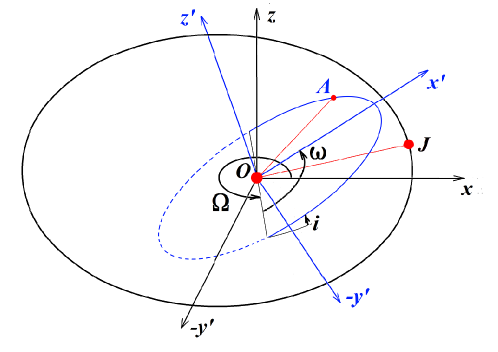
Figure 1: Coordinate frames.

We consider a spatial elliptic restricted three-body problem involving a star $S$, a planet $J$ and an asteroid $A$ (Brouwer & Clemence, 1961). Similar to the frame in Neishtadt & Sheng & Sidorenko (2021), we set the position of the star as the origin $O$ of the Cartesian coordinate system $Oxyz$, and the plane plane $Oxy$ of the system is determined by the motion of the star and the planet. Thus the coordinates of the planet and the asteroid are $(x_{J},y_{J},0)$ and $(x,y,z)$, respectively. The Cartesian coordinate frame $Ox^{\prime}y^{\prime}z^{\prime}$ is a rotating frame of $Oxyz$, where the plane $Ox^{\prime}y^{\prime}$ is the osculating plane of the orbit of the asteroid, then $(x^{\prime},y^{\prime},0)$ are coordinates of the asteroid in the rotating frame. We use the standard osculating elements $a$, $l$, $e$, $\omega$, $i$, $\Omega$ to describe the orbit of the asteroid, which represent the semi-major axis, mean anomaly, eccentricity, argument of periapsis, inclination, and longitude of the ascending node, respectively. See Fig. 1. Then

$$\begin{array}[]{ccl}x&=&\left(\cos\Omega\cos\omega-\cos i\sin\Omega\sin\omega\right)x^{\prime}+\left(-\cos\Omega\sin\omega-\cos i\sin\Omega\cos\omega\right)y^{\prime},\\ y&=&\left(\sin\Omega\cos\omega+\cos i\cos\Omega\sin\omega\right)x^{\prime}+\left(-\sin\Omega\sin\omega+\cos i\cos\Omega\cos\omega\right)y^{\prime},\\ z&=&\left(\sin i\sin\omega\right)x^{\prime}+\left(\sin i\cos\omega\right)y^{\prime}.\end{array}$$ (1)

It follows from Shevchenko (2016), the planet moves in a prescribed elliptic orbit:

$${{x}_{J}}={{a}_{J}}\left(\cos{{E}_{J}}-{{e}_{J}}\right),\ {{y}_{J}}={{a}_{J}}\sqrt{1-{{e}_{J}}^{2}}\,\sin{{E}_{J}},\quad l_{J}=E_{J}-e_{J}\sin E_{J}.$$

Here $a_{J}$, $e_{J}$, $E_{J}$, $l_{J}$ are the semi-major axis, the eccentricity, the eccentric anomaly, and the mean anomaly of the planet’s orbit. We put $a_{J}=1$ for convenient in the following.

3 Hamiltonian of the system

We introduce the canonical Delaunay elements $l$, $g$, $h$, $L$, $G$, $H$, where $l$, $g=\omega$, $h=\Omega$ are the mean anomaly, argument of pericenter ascending node of the asteroid, respectively. $L=\sqrt{(1-\mu)a}$ corresponds to Keplerian energy, $G=L\sqrt{1-e^{2}}$ is the total angular momentum and $H=G\cos i$ is component of angular momentum perpendicular to the equator (Brouwer & Clemence, 1961).

We consider canonical Poincaré variables $p_{1}$, $q_{1}$, $p_{2}$, $q_{2}$, $p_{3}$, $q_{3}$ to demonstrate the dynamics of the asteroid:

$$\begin{array}[]{ll}{{p}_{1}}=L,&{{q}_{1}}=l+g+h,\\ {{p}_{2}}=\sqrt{2\left(L-G\right)}\cos\left(g+h\right),&{{q}_{2}}=-\sqrt{2\left(L-G\right)}\sin\left(g+h\right),\\ {{p}_{3}}=\sqrt{2\left(G-H\right)}\cos h,&{{q}_{3}}=-\sqrt{2\left(G-H\right)}\sin h.\end{array}$$ (2)

Let the mass of the planet be $\mu$ and the mass of the star be $1-\mu$, thus the sum of the mass is $1$. The Hamiltonian of the asteroid is

$$F=-{\frac{\left(1-\mu\right)^{2}}{2{L}^{2}}}+\mu U,$$ (3)

where

$$U=-V=-{\frac{1}{\sqrt{(x-x_{J})^{2}+(y-y_{J})^{2}+{z}^{2}}}}-(x\ddot{x}_{J}+y\ddot{y}_{J})$$ (4)

is the perturbing gravitational potential. In formula (4), the coordinates $(x,y,z)$ of the asteroid can be expressed via Poincaré variables by formulas (1), (2), and equations of motion of the asteroid in the elliptic orbit

$${{x^{\prime}}}={{a}}(\cos E-e),\ {{y^{\prime}}}={{a}}\sqrt{1-{{e}}^{2}}\,\sin{{E}},\quad l=E-e\sin E,$$

where $E$ is the eccentric anomaly of the asteroid. Coordinates $x_{J}$, $y_{J}$ of the planet are prescribed functions of time.

The double averaged Hamiltonian $\bar{F}$ is defined as

$$\bar{F}=\frac{1}{(2\pi)^{2}}\int_{0}^{2\pi}\int_{0}^{2\pi}Fdldl_{J}.$$

It is obvious that

$$\bar{F}=-{\frac{\left(1-\mu\right)^{2}}{2{L}^{2}}}+\mu{\bar{U}}=-{\frac{\left(1-\mu\right)^{2}}{2{L}^{2}}}-\mu{\bar{V}},$$

where $\mu\bar{V}=-\mu\bar{U}$ is the double averaged force function of gravity of the planet:

$$\bar{U}=\frac{1}{(2\pi)^{2}}\int_{0}^{2\pi}\int_{0}^{2\pi}Udldl_{J},\quad U={\frac{1}{\sqrt{(x-x_{J})^{2}+(y-y_{J})^{2}+{z}^{2}}}}.$$

By averaging over the mean anomaly, the double averaged Hamiltonian does not depend on $q_{1}$ anymore, then the canonically conjugate variable $p_{1}=L$ is the first integral of the double averaged system, which means the first term in $\bar{F}$ is constant in the double averaged system. Hence, dynamics of variables $p_{2}$, $q_{2}$, $p_{3}$, $q_{3}$ is described by 2 dimensions of freedom (2-DOF) Hamiltonian system with the Hamiltonian $\mu\bar{U}$. Introducing “slow” time $\tau=\mu t$ as an independent variable, then by transformation, the Hamiltonian of the system becomes $\bar{U}$. It is obvious that $\bar{U}$ depends on the ratio between the semi-major axis of the asteroid and the planet $a$ (we take $a_{J}=1$) and the eccentricity of the planet$e_{J}$ as parameters.

When the inclination $i=0$, the double averaged spacial ER3BP turns to be the case of planer problem, which corresponds to the invariant plane $p_{3}=0,q_{3}=0$. Dynamics in the invariant plane of the system is described by 1-DOF Hamiltonian system with $p_{2}$ and $q_{2}$. Denote the Hamiltonian of the planer problem by $\bar{R}(p_{2},q_{2})$, then $\bar{R}(p_{2},q_{2})=\bar{U}(p_{2},q_{2},p_{3}=0,q_{3}=0)$ is independent of $p_{3}$, $q_{3}$. According to Aksenov (1979) and Neishtadt & Sheng & Sidorenko (2021), the Hamiltonian of the double averaged planer ER3BP is

$$\bar{R}=\frac{1}{(2\pi)^{2}}\int_{0}^{2\pi}\int_{0}^{2\pi}Rdldl_{J},\quad R=-{\frac{1}{\sqrt{(x-x_{J})^{2}+(y-y_{J})^{2}}}}.$$ (5)

We consider the inner case of the double averaged spatial ER3BP. In this case, the distance between the asteroid and the star is much smaller than the distance between the planet and the star. Thus an expansion over the ratio between the semi-major axis of the asteroid and the planet can be established.

The expression of $\bar{R}$ truncated in essential orders is

$$\bar{R}=-1-\frac{a^{2}\left(3e_{A}^{2}+2\right)}{8\left(1-e_{J}^{2}\right)^{\frac{3}{2}}}+\frac{15a^{3}e_{A}e_{J}\left(3e_{A}^{2}+4\right)\cos\!\left(\omega+\Omega\right)}{64\left(1-e_{J}^{2}\right)^{\frac{5}{2}}}.$$ (6)

Thus there exists a branch of orbits with respect to $\Theta=\omega+\Omega$ and the eccentricity of the asteroid $e$. Given some values of the eccentricity of the planet $e_{J}$ and the ratio between the semi-major axis of the asteroid and the planet $a$, we obtain figures of the considered orbits (include equilibria, periodic orbits and other orbits), which coincide with the results in Vashkovyak (1982). The equilibra with respect to $R_{0}$ ($\Theta=0$) is the apsidal alignment case, this case with small inclination $i$ has been studied in Neishtadt & Sheng & Sidorenko (2021) with a conclusion that the asteroid’s orbits are linearly stable. orbits with types of $R_{1}$, $R_{2}$, $R_{3}$, $R_{4}$ are periodic orbits while types of $R_{6}$, $R_{7}$ are other orbits, $R_{5}$ is the bifurcation curve of periodic orbits and other orbits.

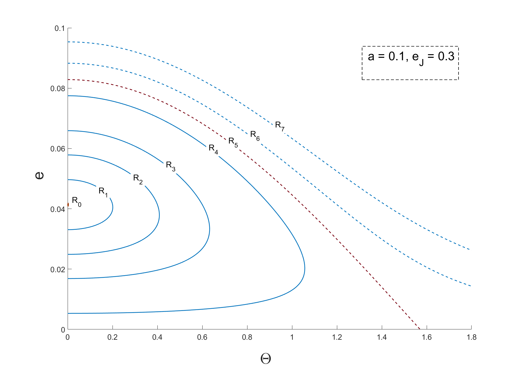
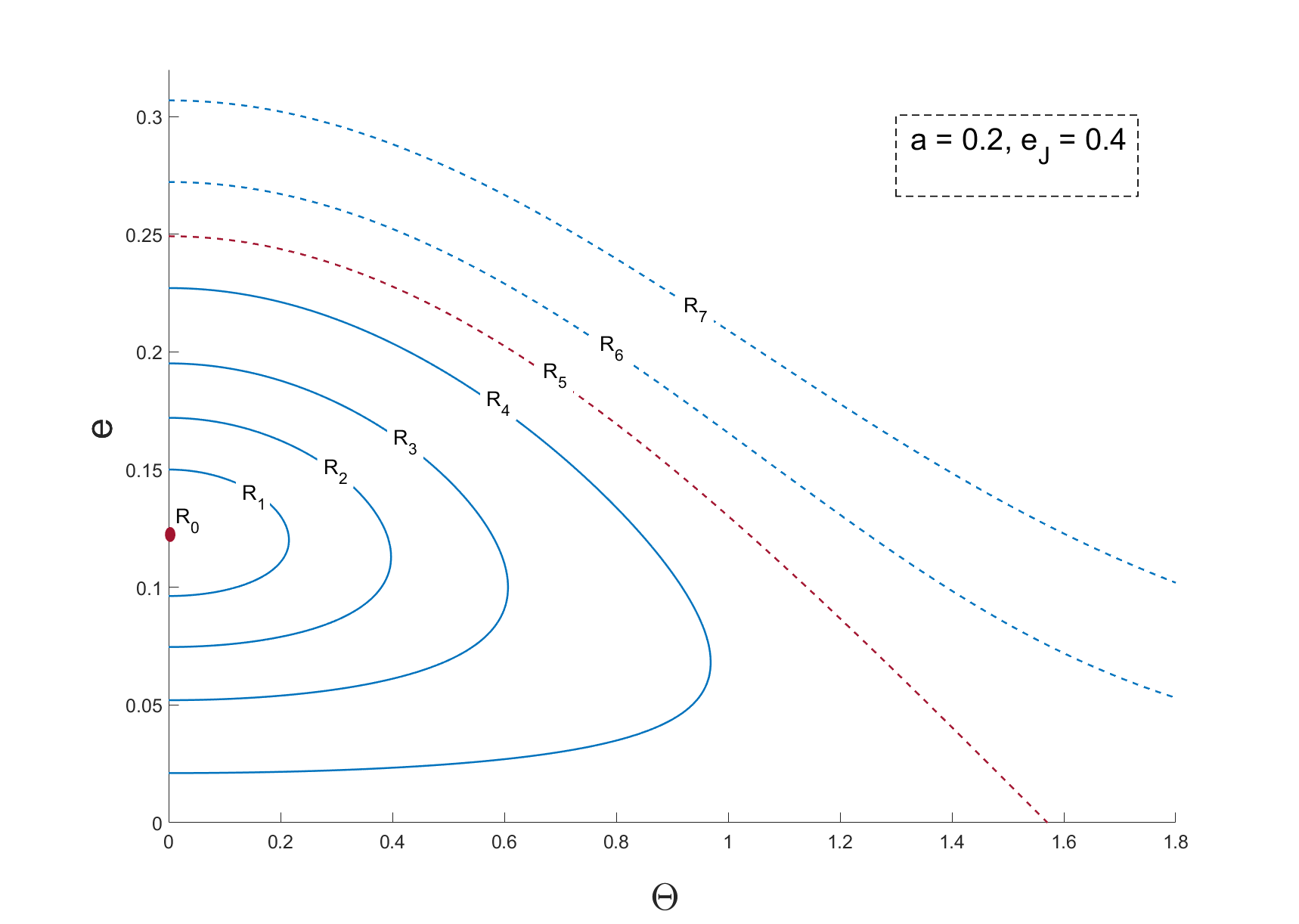
Figure 2: Trajectories of $\Theta$, $e$ in double averaged planar ER3BP.

For spatial problem, denote

$$M_{1}={\frac{{x}^{2}+{y}^{2}+{z}^{2}}{x_{J}^{2}+y_{J}^{2}}},\quad M_{2}=\,-\frac{2\left(xx_{J}+yy_{J}\right)}{x_{J}^{2}+y_{J}^{2}},\quad M=M_{1}+M_{2}\,.$$ (7)

We obtain the approximate formula of force function of gravity $U$ of the planet for this limiting case. Expansion of $U$ up to $a^{3}$ has the form

$$U=-\frac{1}{\sqrt{x_{J}^{2}+y_{J}^{2}}}\left(1-\frac{1}{2}M+\frac{3}{8}\left(M_{1}M_{2}+M_{2}^{2}\right)-\frac{5}{16}M_{2}^{3}\right).$$ (8)

Then we substitute $x$, $x_{J}$, $y$, $y_{J}$ into the above formula and average (8) over $l$, $l_{J}$ to obtain the corresponding expansion of $\bar{U}$. We consider the apsidal alignment case ($\omega+\Omega=0$) and the general case ($\omega+\Omega=\Theta$) of the problem. The potential function $U$ in the spatial ER3BP is a function of $p_{3}$, $q_{3}$ with parameter $\Theta$ and $i$, denoted by $U_{\Theta,i}$. The double averaged potential function $\bar{U}$ is $\bar{U}_{\Theta,i}$. We will study the apsidal alignment case with large inclinations ($U=U_{0,i}$), the general case with small inclinations ($U=U_{\Theta,0^{+}}$), and finally the general case with large inclinations ($U=U_{\Theta,i}$).

4 Stability analysis in apsidal alignment case

It is established numerically by Vashkovyak (1982), as well as Fig 2 in this paper, that the double averaged planar restricted elliptic three-body problem has stationary solutions (equilibria)

$$q_{2}=0,\quad p_{2}=p_{2*},$$ (9)

for some domains in the plane of parameters $a,e_{J}$.

The the equilibria (9) corresponds to the apsidal alignment case in which $\omega+\Omega=0$. We consider a large variation of the inclination $i$ ($-\pi/2<i<\pi/2$), in the planer problem thus turns to be a spatial problem. It is interested to discuss the stability of the orbits of asteroid with respect to an arbitrary inclination $i$.

The expressions of $x$, $y$, $z$ can be simplified as

$$x =\left(1-(1-\cos i)\sin^{2}\Omega\right)x^{\prime}+\left(\cos\Omega\sin\Omega(1-\cos i)\right)y^{\prime},$$ (10)

$$y =\left(\cos\Omega\sin\Omega(1-\cos i)\right)x^{\prime}+\left(1-(1-\cos i)\cos^{2}\Omega\right)y^{\prime},$$

$$z =\left(\sin i\sin\Omega\right)x^{\prime}+\left(\sin i\cos\Omega\right)y^{\prime}.$$

To study linear stability of the equilibria (9) with respect to arbitrary inclination $i$, we need to consider quadratic part of $p_{3}$, $q_{3}$ in the function $\bar{U}_{0,i}$ at these equilibria. Substituting $x$, $y$, $z$ into (8) and taking

$$\cos(\Omega)=\frac{p_{3}}{\sqrt{G\cdot(1-\cos(i))}},\quad\sin(\Omega)=-\frac{q_{3}}{\sqrt{G\cdot(1-\cos(i))}},$$ (11)

from (2), the function $U=U_{0,i}$ with increasing order of $p_{3}$ and $q_{3}$ is

$$U_{0,i}=R_{0,0}+W_{0,i}+O(p_{3}^{4}+q_{3}^{4}),\quad W_{0,i}=\frac{1}{2}\left(Ap_{3}^{2}+2Bp_{3}q_{3}+Cq_{3}^{2}\right),$$ (12)

where

$$A_{0,i} =-\frac{2x^{\prime}x_{J}+2\cos\left(i\right)y^{\prime}y_{J}-\sin\left(i\right)^{2}{y^{\prime}}^{2}}{\left(x_{J}^{2}+y_{J}^{2}\right)^{\frac{3}{2}}G\left(1-\cos\!\left(i\right)\right)}+\frac{3\left(x^{\prime 2}+y^{\prime 2}\right)\left(x^{\prime}x_{J}+\cos\left(i\right)y^{\prime}y_{J}\right)}{\left(x_{J}^{2}+y_{J}^{2}\right)^{\frac{5}{2}}G\left(1-\cos\!\left(i\right)\right)},$$ (13)

$$B_{0,i} =\frac{\sin\left(i\right)^{2}x^{\prime}y^{\prime}-\cos\left(i\right)x^{\prime}y_{J}-\cos\left(i\right)x_{J}y^{\prime}+x^{\prime}y_{J}+x_{J}y^{\prime}}{\left(x_{J}^{2}+y_{J}^{2}\right)^{\frac{3}{2}}G\left(1-\cos\!\left(i\right)\right)}-\frac{3\left(x^{\prime 2}+y^{\prime 2}\right)\left(x^{\prime}y_{J}+x_{J}y^{\prime}\right)}{2\left(x_{J}^{2}+y_{J}^{2}\right)^{\frac{5}{2}}G},$$

$$C_{0,i} =\frac{x^{\prime 2}\sin\!\left(i\right)^{2}-2x^{\prime}x_{J}\cos\!\left(i\right)-2y^{\prime}y_{J}}{\left(x_{J}^{2}+y_{J}^{2}\right)^{\frac{3}{2}}G\left(1-\cos\!\left(i\right)\right)}+\frac{3\left(x^{\prime 2}+y^{\prime 2}\right)\left(x^{\prime}x_{J}\cos\!\left(i\right)+y^{\prime}y_{J}\right)}{\left(x_{J}^{2}+y_{J}^{2}\right)^{\frac{5}{2}}G\left(1-\cos\!\left(i\right)\right)},$$

and $R_{0,0}$ is zero order terms of $p_{3}$ and $q_{3}$, which is not important here.

We consider the double average value of the coefficients in quadratic part of $p_{3}$ and $q_{3}$. Averaging $W_{0,i}$ over the mean anomaly of the asteroid $l$ and the mean anomaly of the planet $l_{J}$, we have

$$\bar{W}_{0,i}=\frac{1}{2}\left(\bar{A}\,{p}_{3}^{2}+2\bar{B}p_{3}q_{3}+\bar{C}\,{q}_{3}^{2}\right),$$ (14)

where

$$\bar{A}_{0,i}=\frac{1}{{4{\pi}^{2}}}\int_{0}^{2\pi}\int_{0}^{2\pi}\left(A_{0,i}\right)\text{d}l\text{d}{l}_{J},$$ (15)

$$\bar{B}_{0,i}=\frac{1}{{4{\pi}^{2}}}\int_{0}^{2\pi}\int_{0}^{2\pi}\left(B_{0,i}\right)\text{d}l\text{d}{l}_{J},$$

$$\bar{C}_{0,i}=\frac{1}{{4{\pi}^{2}}}\int_{0}^{2\pi}\int_{0}^{2\pi}\left(C_{0,i}\right)\text{d}l\text{d}{l}_{J}$$

are the average values of $A_{0,i}$, $B_{0,i}$ and $C_{0,i}$.

We have eccentric anomaly $E$ of the asteroid in our formulas of $x$, $y$ and eccentric anomaly $E_{J}$ of the planet in $x_{J}$, $y_{J}$. By Kepler’s equation

$$l=E-e\sin E,\,\,\,l_{J}=E_{J}-e\sin E_{J},$$ (16)

then for any function $f$ we have

$$\frac{1}{{4{\pi}^{2}}}\int_{0}^{2\pi}{}\int_{0}^{2\pi}{f}\text{d}l\text{d}{{l}_{J}} =\frac{1}{{4{\pi}^{2}}}\int_{0}^{2\pi}{}\int_{0}^{2\pi}{f}\frac{\text{d}{{l}}}{\text{d}{{E}}}\frac{\text{d}{{l}_{J}}}{\text{d}{{E}_{J}}}{\text{d}E}\text{d}{{E}_{J}}$$ (17)

$$=\frac{1}{{4{\pi}^{2}}}\int_{0}^{2\pi}{}\int_{0}^{2\pi}{f}\left(1-e\cos E\right)\left(1-{{e}_{J}}\cos{{E}_{J}}\right)\text{d}E\text{d}{{E}_{J}}.$$

Thus the averaging values $\bar{A}_{0,i}$, $\bar{B}_{0,i}$ and $\bar{C}_{0,i}$ can be written as

$$\bar{A}_{0,i}=\frac{1}{{4{\pi}^{2}}}\int_{0}^{2\pi}\int_{0}^{2\pi}\left(A_{0,i}\right)\left(1-e\cos E\right)\left(1-{{e}_{J}}\cos{{E}_{J}}\right)\text{d}E\text{d}{E}_{J},$$ (18)

$$\bar{B}_{0,i}=\frac{1}{{4{\pi}^{2}}}\int_{0}^{2\pi}\int_{0}^{2\pi}\left(B_{0,i}\right)\left(1-e\cos E\right)\left(1-{{e}_{J}}\cos{{E}_{J}}\right)\text{d}E\text{d}{E}_{J},$$

$$\bar{C}_{0,i}=\frac{1}{{4{\pi}^{2}}}\int_{0}^{2\pi}\int_{0}^{2\pi}\left(C_{0,i}\right)\left(1-e\cos E\right)\left(1-{{e}_{J}}\cos{{E}_{J}}\right)\text{d}E\text{d}{E}_{J}.$$

We substitute $x^{\prime}$, $y^{\prime}$, $x_{J}$, $y_{J}$ into the above formula, it is calculated that the value of $\bar{B}_{0,i}$ is always $0$, and

$$\bar{A}_{0,i}=\frac{\left(1-e^{2}\right)\sin\!\left(i\right)^{2}a^{2}}{4G\left(1-\cos\!\left(i\right)\right)\left(1-e_{J}^{2}\right)^{\frac{3}{2}}}-\frac{15e_{J}\left(4+3e^{2}\right)ea^{3}}{16G\left(1-\cos\!\left(i\right)\right)\left(1-e_{J}^{2}\right)^{\frac{5}{2}}},$$ (19)

$$\bar{C}_{0,i}=\frac{\left(1+4e^{2}\right)\sin\!\left(i\right)^{2}a^{2}}{4G\left(1-\cos\!\left(i\right)\right)\left(1-e_{J}^{2}\right)^{\frac{3}{2}}}-\frac{15e_{J}\cos\!\left(i\right)\left(4+3e^{2}\right)e_{A}a^{3}}{16G\left(1-\cos\!\left(i\right)\right)\left(1-e_{J}^{2}\right)^{\frac{5}{2}}}.$$

It is obvious that $\bar{A}_{0,i}>0$ and $\bar{C}_{0,i}>0$ for sufficiently small $a$, thus $\bar{W}_{0,i}$ is a positive definite quadratic form. Hence, stable equilibria of the double averaged planar restricted elliptic three-body problem are stable in the linear approximation as equilibria of the double averaged spatial restricted elliptic three-body problem for all values of parameters. Numerical simulation is shown in Fig. 3 with $e_{J}=0.3$, $a=0.1$, and the corresponding equilibrium is $\Theta=0$, $e=0.041367$.

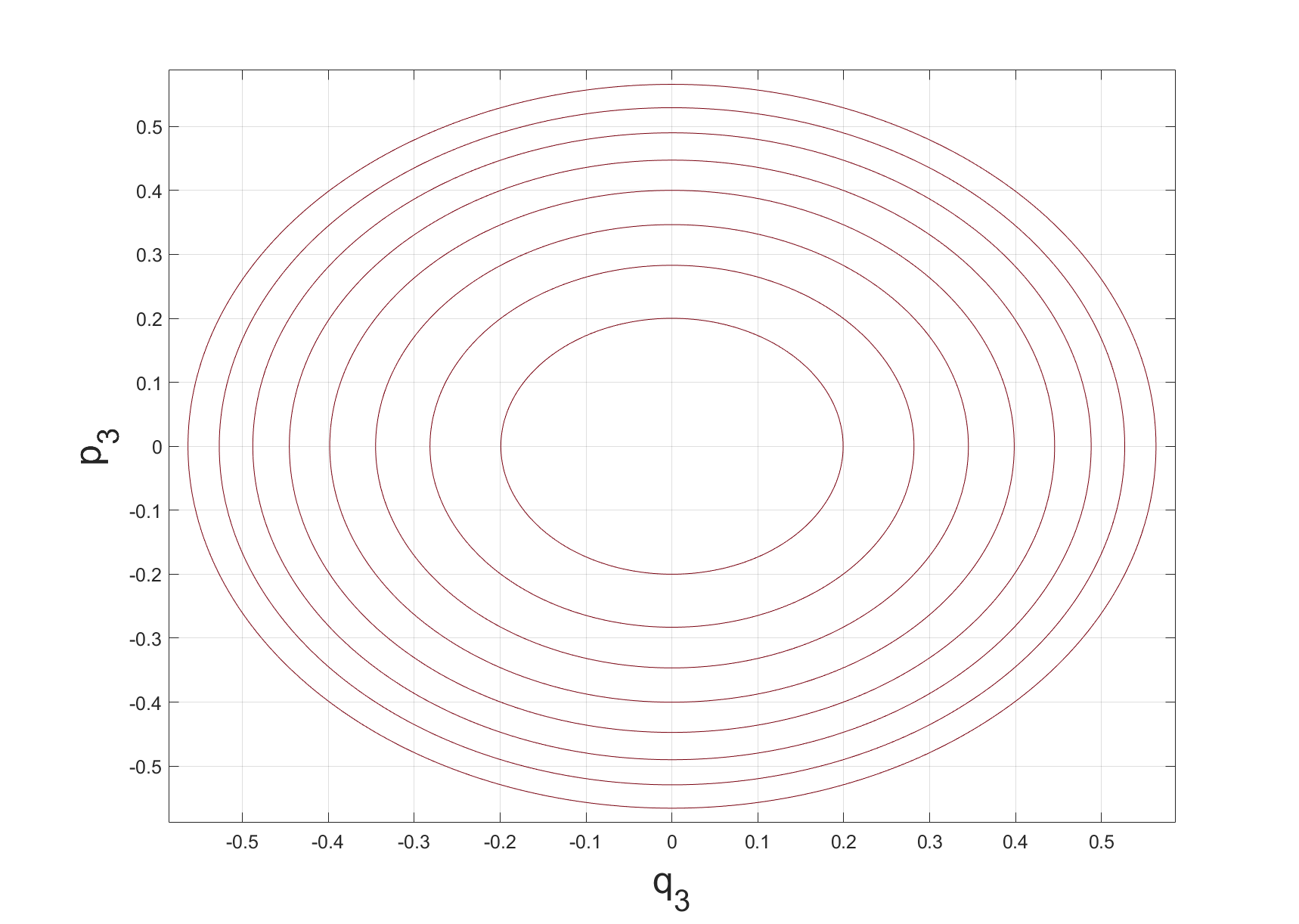
Figure 3: Phase portrait of $p_{3}$, $q_{3}$ in apsidal alignment case.

It is known that the double averaged planar ER3BP corresponds to the invariant plane $i=0$. However, the asteroid can not cross the invariant plane without external forces. This is because that the vertical angular momentum $H$ is also conserved in the system in addition to the total energy (Naoz et al., 2013). Since $H=G\cos i$ is a constant, and $G$ is always positive, the test particle should always be in a prograde orbit or always be in a retrograde orbit so that $\cos i$ do not change its sign. Thus, given a large perturbation of the inclination $i$ in the above problem, the orbits of the asteroid will return to the invariant plane with infinite time. Although the system can not reach the equilibrium in finite time, a situation of small inclination $i$ is able to appear, which is the case has been studied in Neishtadt & Sheng & Sidorenko (2021) with a result of linear stability.

5 Stability analysis in small perturbation case

The equilibria (9) corresponds to the apsidal alignment case in which $\omega+\Omega=0$. Vashkovyak (1982) and Fig 2 in this paper demonstrated that there are period orbits and other orbits around the equilibria (9), which correspond to $\Theta=\omega+\Omega\neq 0$. Thus consideration of general cases (i.e. $\Theta\neq 0$) is useful to establish the linear stability of the asteroid’s orbits.

We consider the small perturbation case initially, which means the inclination $i$ is regarded as the small perturbation. In this case, the formula of $x$, $y$ and $z$ can be obtained with $i=0$ and $\omega+\Omega=\Theta$, thus we have $z=0$ and

$$x =\cos(\Theta)x^{\prime}-\sin(\Theta)y^{\prime},$$ (20)

$$y =\sin(\Theta)x^{\prime}+\cos(\Theta)y^{\prime}.$$

Formula (11) can be expanded as

$$\cos(\Omega)=\frac{p_{3}}{\sqrt{G\cdot i^{2}/2}},\quad\sin(\Omega)=-\frac{q_{3}}{\sqrt{G\cdot i^{2}/2}}.$$ (21)

Substituting $x$, $y$ and $z=0$ into (8), the function $U=U_{\Theta,0^{+}}$ with increasing order of $p_{3}$ and $q_{3}$ can be written as

$$U_{\Theta,0^{+}}=R_{\Theta,0^{+}}+W_{\Theta,0^{+}}+O(p_{3}^{4}+q_{3}^{4}),\quad W_{\Theta,0^{+}}=\frac{1}{2}\left(A_{\Theta,0^{+}}p_{3}^{2}+2B_{\Theta,0^{+}}p_{3}q_{3}+C_{\Theta,0^{+}}q_{3}^{2}\right),$$ (22)

where

$$A_{\Theta,0^{+}} =\,\frac{y{{y}_{J}}}{G{\left[{\left(x-{{x}_{J}}\right)}^{2}+{{\left(y-{{y}_{J}}\right)}^{2}}\right]}^{{3}/{2}}},$$ (23)

$$B_{\Theta,0^{+}} =\,\frac{\left(x{{y}_{J}}+y{{x}_{J}}\right)}{2G{{\left[{{\left(x-{{x}_{J}}\right)}^{2}}+{{\left(y-{{y}_{J}}\right)}^{2}}\right]}^{{3}/{2}}}},$$

$$C_{\Theta,0^{+}} =\,\frac{x{{x}_{J}}}{G{\left[{{\left(x-{{x}_{J}}\right)}^{2}}+{{\left(y-{{y}_{J}}\right)}^{2}}\right]^{{3}/{2}}}}.$$

Calculations are similar to the procedure in Neishtadt & Sheng & Sidorenko (2021).

We consider the double average value of the coefficients in quadratic form of $p_{3}$ and $q_{3}$, and average $W_{\Theta,0^{+}}$ with the same procedure in (17), then

$$\bar{W}_{\Theta,0^{+}}=\frac{1}{2}\left(\bar{A}_{\Theta,0^{+}}\,{{p}_{3}}^{2}+2\bar{B}_{\Theta,0^{+}}p_{3}q_{3}+\bar{C}_{\Theta,0^{+}}\,{{q}_{3}}^{2}\right),$$ (24)

where $\bar{A}_{\Theta,0^{+}}$, $\bar{B}_{\Theta,0^{+}}$ and $\bar{C}_{\Theta,0^{+}}$ are the average values of $A_{\Theta,0^{+}}$, $B_{\Theta,0^{+}}$ and $C_{\Theta,0^{+}}$ respectively by the averaging method in formula (LABEL:barAC0) and (LABEL:barAC).

Substituting $x^{\prime}$, $y^{\prime}$, $x_{J}$, $y_{J}$ into the double average value of the coefficients, we obtain

$$\bar{A}_{\Theta,0^{+}}= -\frac{3a^{2}\left(5\cos\!\left(\Theta\right)^{2}e_{A}^{2}-4e_{A}^{2}-1\right)}{4G\left(-e_{J}^{2}+1\right)^{\frac{3}{2}}}+\frac{75a^{3}e_{A}e_{J}\cos\!\left(\Theta\right)\left(7\cos\!\left(\Theta\right)^{2}e_{A}^{2}-6e_{A}^{2}-1\right)}{32\sqrt{-e_{J}^{2}+1}\,G\left(e_{J}-1\right)^{2}\left(e_{J}+1\right)^{2}}+O(a^{4}),$$ (25)

$$\bar{B}_{\Theta,0^{+}}= \frac{15a^{2}e_{A}^{2}\cos\!\left(\Theta\right)\sin\!\left(\Theta\right)}{4G\left(-e_{J}^{2}+1\right)^{\frac{3}{2}}}-\frac{15e_{A}a^{3}\sin\!\left(\Theta\right)e_{J}\left(140\cos\!\left(\Theta\right)^{2}e_{A}^{2}-17e_{A}^{2}+24\right)}{128\sqrt{-e_{J}^{2}+1}\,G\left(e_{J}-1\right)^{2}\left(e_{J}+1\right)^{2}}+O(a^{4}),$$

$$\bar{C}_{\Theta,0^{+}}= \frac{3a^{2}\left(5\cos\!\left(\Theta\right)^{2}e_{A}^{2}-e_{A}^{2}+1\right)}{4G\left(-e_{J}^{2}+1\right)^{\frac{3}{2}}}-\frac{15a^{3}\cos\!\left(\Theta\right)e_{A}e_{J}\left(70\cos\!\left(\Theta\right)^{2}e_{A}^{2}-27e_{A}^{2}+34\right)}{64G\left(-e_{J}^{2}+1\right)^{\frac{5}{2}}}+O(a^{4}).$$

In above formulas, terms of higher order of $a$ are omitted. As well as $a$ is small enough, we only need the terms of $a^{2}$ in formula (25).

It is obvious that $\bar{A}_{\Theta,0^{+}}>0$ and $\bar{C}_{\Theta,0^{+}}>0$, and

$$D_{\Theta,0^{+}}=\det\left[\begin{array}[]{cc}\bar{A}_{\Theta,0^{+}}&\bar{B}_{\Theta,0^{+}}\\ \bar{B}_{\Theta,0^{+}}&\bar{C}_{\Theta,0^{+}}\end{array}\right]=\frac{9a^{4}\left(1+3e_{A}^{2}-4e_{A}^{4}\right)}{16G^{2}\left(1-e_{J}^{2}\right)^{3}}>0.$$ (26)

These conditions provide a linear stability of the orbits of the asteroid in small perturbation case, which means stable periodic orbits of the double averaged planar restricted elliptic three-body problem are stable in the linear approximation as periodic orbits of the double averaged spatial restricted elliptic three-body problem with small inclination for all values of parameters.

6 Expansion of the problem for general inner case

The spatial perturbation of the asteroid’s orbits may not be small, as we discussed in previous section, large variations of the inclination $i$ are of great interest. In this section we consider the problem with large perturbation, i.e. inclination $i$ is not small.

For general situation, we have $\omega+\Omega=\Theta$ in the formula of $x$,$y$ and $z$. Thus

$$x =\left(\cos\Omega\cos(\Theta-\omega)-\cos i\sin\Omega\sin(\Theta-\omega)\right)x^{\prime}+\left(-\cos\Omega\sin(\Theta-\omega)-\cos i\sin\Omega\cos(\Theta-\omega)\right)y^{\prime},$$ (27)

$$y =\left(\sin\Omega\cos(\Theta-\omega)+\cos i\cos\Omega\sin(\Theta-\omega)\right)x^{\prime}+\left(-\sin\Omega\sin(\Theta-\omega)+\cos i\cos\Omega\cos(\Theta-\omega)\right)y^{\prime},$$

$$z =\left(\sin i\sin(\Theta-\omega)\right)x^{\prime}+\left(\sin i\cos(\Theta-\omega)\right)y^{\prime}.$$

We still take

$$\cos(\Omega)=\frac{p_{3}}{\sqrt{G\cdot(1-\cos(i))}},\quad\sin(\Omega)=-\frac{q_{3}}{\sqrt{G\cdot(1-\cos(i))}}$$

from (2). Substituting $x$, $y$, $z$ into (8), the function $U_{\Theta}$ with increasing order of $p_{3}$ and $q_{3}$ can be written as

$$U_{\Theta,i}=R_{\Theta,i}+W_{\Theta,i}+O(p_{3}^{4}+q_{3}^{4}),\quad W_{\Theta,i}=\frac{1}{2}\left(A_{\Theta,i}p_{3}^{2}+2B_{\Theta,i}p_{3}q_{3}+C_{\Theta,i}q_{3}^{2}\right),$$ (28)

where

$$A_{\Theta,i}= \frac{\sin\left(i\right)^{2}y\left(0\right)^{2}-2\cos\left(i\right)y\left(0\right)y_{J}-2x\left(0\right)x_{J}}{\left(x_{J}^{2}+y_{J}^{2}\right)^{\frac{3}{2}}G\left(1-\cos\!\left(i\right)\right)}+O(a^{3}),$$ (29)

$$B_{\Theta,i}= \frac{\sin\left(i\right)^{2}x\left(0\right)y\left(0\right)}{\left(x_{J}^{2}+y_{J}^{2}\right)^{\frac{3}{2}}G\left(1-\cos\left(i\right)\right)}+\frac{x\left(0\right)y_{J}+x_{J}y\left(0\right)}{\left(x_{J}^{2}+y_{J}^{2}\right)^{\frac{3}{2}}G}+O(a^{3}),$$

$$C_{\Theta,i}= \frac{\sin\left(i\right)^{2}x\left(0\right)^{2}-2\cos\left(i\right)x\left(0\right)x_{J}-2y\left(0\right)y_{J}}{\left(x_{J}^{2}+y_{J}^{2}\right)^{\frac{3}{2}}G\left(1-\cos\left(i\right)\right)}+O(a^{3}).$$

In above formulas, terms of higher order of $a$ are omitted, $x\left(0\right)$, $y\left(0\right)$ are values of $x$, $y$ with respect to the planer problem, i.e. $i=0$. We have

$$x\left(0\right) =\cos\left(\Theta\right)x^{\prime}-\sin\left(\Theta\right)y^{\prime},$$ (30)

$$y\left(0\right) =\sin\left(\Theta\right)x^{\prime}+\cos\left(\Theta\right)y^{\prime}.$$

We consider the double average value of the coefficients in quadratic form of $p_{3}$ and $q_{3}$, and average $W_{\Theta,i}$ with the same procedure in (17), then

$$\bar{W}_{\Theta,i}=\frac{1}{2}\left(\bar{A}_{\Theta,i}\,{{p}_{3}}^{2}+2\bar{B}_{\Theta,i}p_{3}q_{3}+\bar{C}_{\Theta,i}\,{{q}_{3}}^{2}\right),$$ (31)

where

$$\bar{A}_{\Theta,i}=\frac{1}{{4{\pi}^{2}}}\int_{0}^{2\pi}\int_{0}^{2\pi}\left(A_{\Theta,i}\right)\left(1-e\cos E\right)\left(1-{{e}_{J}}\cos{{E}_{J}}\right)\text{d}E\text{d}{E}_{J},$$ (32)

$$\bar{B}_{\Theta,i}=\frac{1}{{4{\pi}^{2}}}\int_{0}^{2\pi}\int_{0}^{2\pi}\left(B_{\Theta,i}\right)\left(1-e\cos E\right)\left(1-{{e}_{J}}\cos{{E}_{J}}\right)\text{d}E\text{d}{E}_{J},$$

$$\bar{C}_{\Theta,i}=\frac{1}{{4{\pi}^{2}}}\int_{0}^{2\pi}\int_{0}^{2\pi}\left(C_{\Theta,i}\right)\left(1-e\cos E\right)\left(1-{{e}_{J}}\cos{{E}_{J}}\right)\text{d}E\text{d}{E}_{J}$$

are the average values of $A_{\Theta,i}$, $B_{\Theta,i}$ and $C_{\Theta,i}$.

Substituting $x^{\prime}$, $y^{\prime}$, $x_{J}$, $y_{J}$ into the double average value of the coefficients, we obtain

$$\bar{A}_{\Theta,i} =\frac{\sin\!\left(i\right)^{2}a^{2}\left(1+4e^{2}-5\cos\!\left(\Theta\right)^{2}e^{2}\right)}{4G\left(1-e_{J}^{2}\right)^{\frac{3}{2}}\left(1-\cos\left(i\right)\right)},$$ (33)

$$\bar{B}_{\Theta,i} =\frac{5\sin\!\left(i\right)^{2}\cos\!\left(\Theta\right)\sin\!\left(\Theta\right)a^{2}e^{2}}{4G\left(1-e_{J}^{2}\right)^{\frac{3}{2}}\left(1-\cos\left(i\right)\right)},$$

$$\bar{C}_{\Theta,i} =\frac{\sin\!\left(i\right)^{2}a^{2}\left(5\cos\!\left(\Theta\right)^{2}e^{2}-e^{2}+1\right)}{4G\left(1-e_{J}^{2}\right)^{\frac{3}{2}}\left(1-\cos\left(i\right)\right)}.$$

It is obvious that $\bar{A}_{\Theta,i}>0$ and $\bar{C}_{\Theta,i}>0$, and we have

$$D_{\Theta,i}=\det\left[\begin{array}[]{cc}\bar{A}_{\Theta,i}&\bar{B}_{\Theta,i}\\ \bar{B}_{\Theta,i}&\bar{C}_{\Theta,i}\end{array}\right]=\frac{a^{4}\sin\left(i\right)^{4}\left(1+3e^{2}-4e^{4}\right)}{16G^{2}\left(1-e_{J}^{2}\right)^{3}\left(1-\cos\left(i\right)\right)^{2}}>0.$$ (34)

In absence of variable $\Theta$, formula (34) holds for any values of $e$. The sequential principal minor $\bar{A}_{\Theta,i}>0$ and $\bar{A}_{\Theta,i}\bar{C}_{\Theta,i}-\bar{B}_{\Theta,i}^{2}>0$, thus $\bar{W}_{\Theta,i}$ is a positive definite quadratic form, which guaranteed the linear stability of the orbits of the asteroid. Hence, given a stable periodic orbits of the double averaged planar restricted elliptic three-body problem, linear stability is kept for the periodic orbits of the double averaged spatial restricted elliptic three-body problem with large perturbation over inclination $i$ for all values of parameters. When $\Theta=0$, the problem corresponds to the apsidal alignment case, the conclusion coincides with the results in previous section.

Numerical examples of phase portraits of the system for canonical variables $p_{3}$ and $q_{3}$ with periodic orbits and other orbits of parameters $\Theta$ and $e$ are shown in Fig. 4 and Fig. 5 respectively. The changing of values of $e$ in the same orbit cause small influence of the phase curves, and does not break the linear stability.

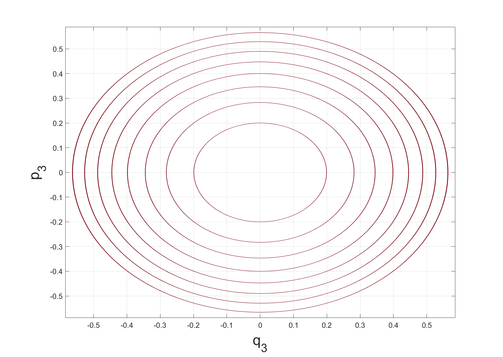
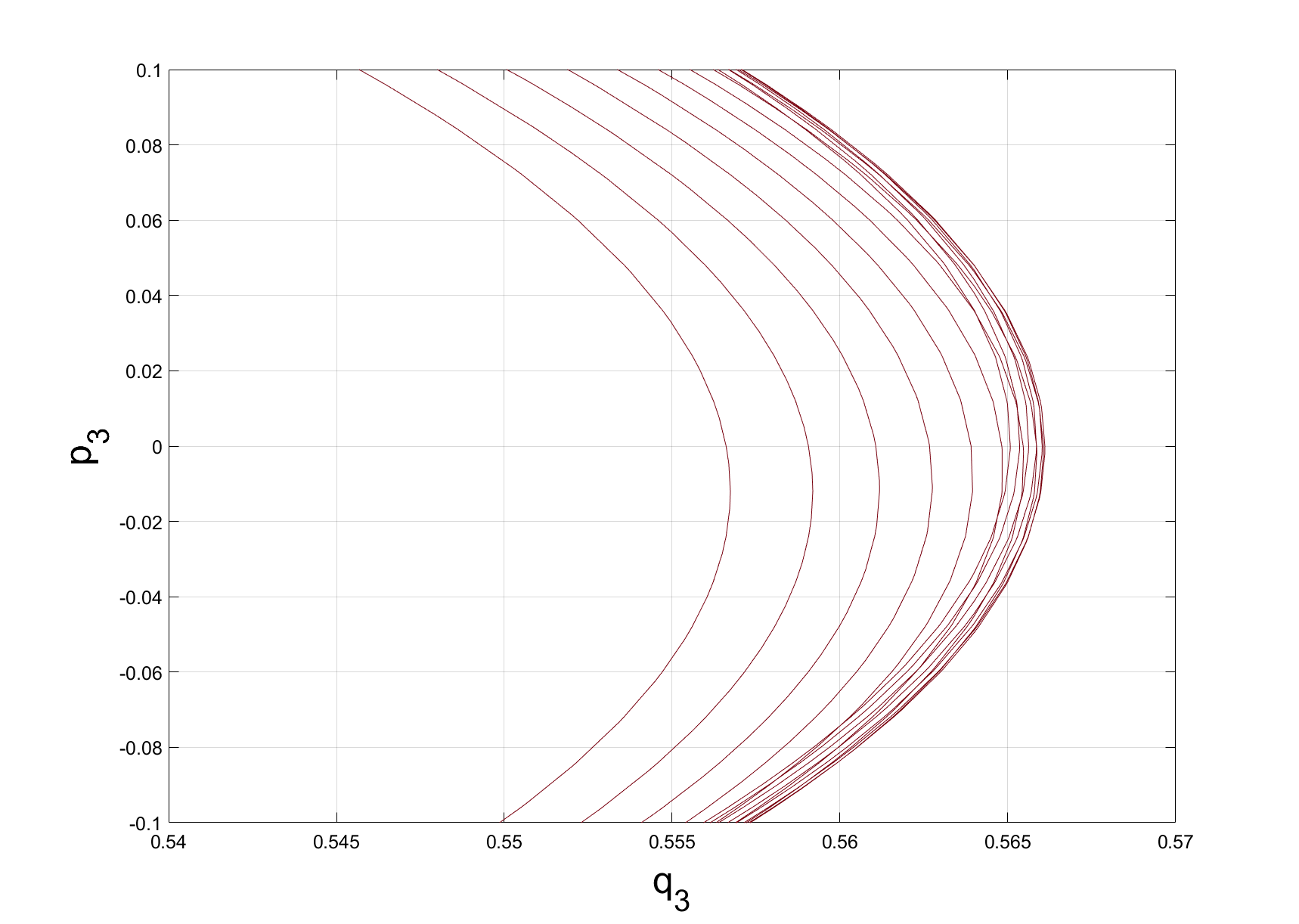
Figure 4: Phase portrait of $p_{3}$, $q_{3}$ with periodic orbits of $\Theta$ and $e$.

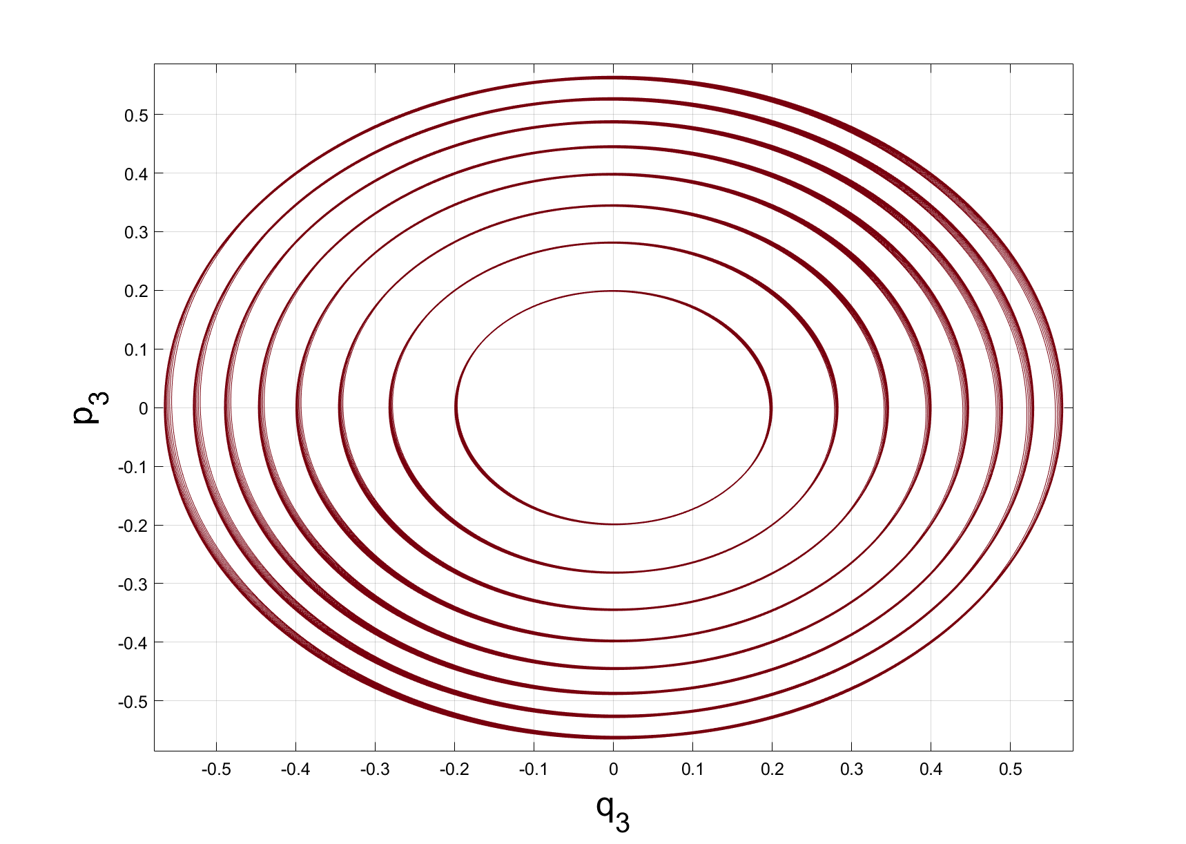
Figure 5: Phase portrait of $p_{3}$, $q_{3}$ with other orbits of $\Theta$ and $e$.

Similar to the explanation in apsidal alignment case, the orbits of the asteroid can not cross the invariant plane and will return to the invariant plane in finite time. Thus in finite time, the problem will degenerate to the small perturbation case, which is studied in last section.

We only considered the double averaged spatial restricted elliptic three-body problem with the inclination $-\pi/2<i<\pi/2$, for values of $i$ between $(\pi/2,\pi)$ and $(-\pi/2,-\pi/2)$, one can choose the corresponding equilibra in apsidal contrary case, and perform a similar calculation.

We only consider the linear stability in this work, Lidov - Kozai effect resulted in a large coupled periodic changes of the eccentricity and the inclination of a natural or artificial celestial body, thus the asteroid’s orbits may not prevent the stability if there are nonlinear instability or resonances instability between frequencies of the eccentricity and the inclination. Most natural or artificial celestial bodies have small eccentricities and inclinations, the mentioned resonances instability hardly occur, thus study the linear stability of periodic orbits around the apsidal alignment equilibra (9) are of great importance. A further discussion is needed to determine the nonlinear stability for the problem, which is an open question. The analysis of the nonlinear stability as well as the resonance cases can be a direction of the future work.

7 Conclusion

We have analyzed the secular effects in the motion of an asteroid with negligible mass in inner case of a spatial restricted elliptic three-body problem with arbitrary inclination. Linear stability of the asteroid’s orbits are studied. It is showed that equilibra, periodic orbits and other orbits of the double averaged planar restricted elliptic three-body problem are stable in the linear approximation as those orbits of the double averaged spatial restricted elliptic three-body problem with arbitrary inclination for all values of parameters. Numerical simulations of different orbits coincide with our results as well. This model with large eccentricities of the planet is of particular interest in relation to study of motion of exoplanets.

References

• Aksenov (1979) Aksenov, E.P.: The doubly averaged, elliptical, restricted, three-body problem. Sov. Astronomy 23, 236-240 (1979)
• Arnold (1961) Arnold, V.I.: The stability of the equilibrium position of a Hamiltonian system of ordinary differential equations in the general elliptic case. Sov. Math., Dokl. 2, 247–249 (1961)
• Arnold et al. (2006) Arnold, V.I., Kozlov, V.V., Neishtadt, A.I.: Mathematical Aspects of Classical and Celestial Mechanics, 3rd edn. Springer, New York (2006)
• Brouwer & Clemence (1961) Brouwer, D., Clemence, G.M.: Methods of Celestial Mechanics. Academic Press, New York (1961)
• Harrington (1968) Harrington, R.S.: Dynamical evolution of triple stars. Astron. J. 73, 190-194 (1968)
• Huang & Lei (2022) Huang, X., Lei, H. . Orbital Flips Caused by the Eccentric Von Zeipel–Lidov–Kozai Effect in Nonrestricted Hierarchical Planetary Systems. The Astronomical Journal, 164 (2022).
• Katz et al. (2011) Katz, B., Dong, S., Malhotra, R.: Long-term cycling of Kozai–Lidov cycles: extreme eccentricities and inclinations excited by a distant eccentric perturber. Phys. Rev. Lett. 107, 181101 (2011)
• Kozai (1962) Kozai, Y.: Secular perturbations of asteroids with high inclination and eccentricity. Astron. J. 67. 591-598 (1962)
• Lei (2022) Lei, H. . A Systematic Study about Orbit Flips of Test Particles Caused by Eccentric Von Zeipel–Lidov–Kozai Effects. The Astronomical Journal, 163 (2022).
• Leontovich (1962) Leontovich, A.M.: On the stability of the Lagrange periodic solutions of the restricted problem of three bodies. Sov. Math. Dokl. 3, 425–428 (1962)
• Lidov (1962) Lidov, M.L.: The evolution of orbits of artificial satellites of planets under the action of gravitational perturbations of external bodies. Planet. Space Sci. 9. 719-759 (1962)
• Lidov & Ziglin (1974) Lidov, M.L., Ziglin, S.L.: The analysis of restricted circular twice-averaged three body problem in the case of close orbits. Celest. Mech. 9, 151-173 (1974)
• Lithwick & Naoz (2011) Lithwick, Y., Naoz, S.: The eccentric Kozai mechanism for a test particle. Astrophys. J. 742:94 (2011)
• Markeev (1968) Markeev, A.P.: Stability of a canonical system with two degrees of freedom in the presence of resonance. Journal of Applied Mathematics and Mechanics. 41. 225-235 (1977)
• Michtchenko & Malhotra (2004) Michtchenko, T.F., Malhotra, R.: Secular dynamics of the three-body problem: application to the $\upsilon$ Andromedae planetary system. ICARUS. 168. 237-248 (2004)
• Moiseev (1945) Moiseev, N.D.: On some fundamental simplified schemes of celestial mechanics obtained by averaging of the restricted three-points problem. 2. On the averaged versions of the three-dimensional restricted circular three-points problem. Trudy GAISh 15. 100-117 (1945) (in Russian)
• Moser (1968) Moser, J.: Lectures on Hamiltonian Systems. Mem. Am. Math. Soc. 81. American Mathematical Society, Providence, R. I. (1968)
• Naoz (2016) Naoz, S.: The eccentric Kozai–Lidov effect and its applications. Ann. Rev. Astron. Astrophys. 54, 441–489 (2016)
• Naoz et al. (2013) Naoz, S., Farr, W. M., Lithwick, Y., Rasio, F. A., Teyssandier, J. (2013). Secular dynamics in hierarchical three-body systems. Monthly Notices of the Royal Astronomical Society, 431(3), 2155-2171.
• Neishtadt (1975) Neishtadt, A.I.: Stability of plane solutions in the doubly averaged restricted circular three-body problem. Soviet Astronomy Letters 1. 211-213 (1975)
• Neishtadt & Sheng & Sidorenko (2021) Neishtadt, A.I., Sheng, K., Sidorenko, V.V.: Stability analysis of apsidal alignment in double-averaged restricted elliptic three-body problem. Celest. Mech. Dyn. Astr. 133:45 (2021)
• Palacián et al. (2006) Palacián, J.F., Yanguas, P., Fernández, S., Nicotra, M.A.: Searching for periodic orbits of the spatial elliptic restricted three-body problem by double averaging. Physica D. 213. 15-24 (2006)
• Shevchenko (2016) Shevchenko, I.: The Lidov-Kozai Effect - Applications in Exoplanet Research and Dynamical Astronomy. Springer, Berlin (2016)
• Sidorenko (2018) Sidorenko, V.V.: The eccentric Kozai-Lidov effect as a resonance phenomenon. Celest. Mech. Dyn. Astr. 134:4 (2018)
• Sokolskii (1974) Sokolskii, A.G.: On the stability of an autonomous Hamiltonian system with two degrees of freedom in the case of equal frequencies. Journal of Applied Mathematics and Mechanics, 38. 741-749 (1974)
• Stephen et al. (2012) Stephen, R.K., David, R.C., Dawn, M.G., Kaspar, V.B.: The exoplanet eccentricity distribution from Kepler planet candidates. MNRAS 425. 757 - 762 (2012)
• Subaru Telescope Team (2017) Subaru Telescope Team: Inclined Orbits Prevail in Exoplanetary Systems.
$https://www.subarutelescope.org/Pressrelease/2010/12/20/index.html$ (2017)
• Vashkovyak (1981) Vashkovyak, M.A.: Evolution of orbits in the restricted circular twice-averaged-three body problem. I. Qualitative investigations. Cosm. Res. 19. 1–10 (1981)
• Vashkovyak (1982) Vashkovyak, M A.: Evolution of orbits in the two-dimensional restricted elliptical twice-averaged three-body problem. Cosmic Research, 20. 236-244 (1982)
• von Zeipel (1910) von Zeipel, H.: Sur l’application des séries de M. Lindstedt à l’étude du mouvement des cométes pèriodiques. Astronomische Nachrichten 1983. 345 - 418 (1910)
• Ziglin (1975) Ziglin, S.L.: Secular evolution of the orbit of a planet in a binary-star system. Sov. Astron. Lett. 1. 194-195 (1975)
• Ziglin & Lidov (1977) Ziglin, S.L, Lidov, M.L.: Hill’s case of the averaged problem of three bodies and the stability of plane orbits. Journal of Applied Mathematics and Mechanics 41. 225-235 (1977)