Multi-Agent Path Finding with Continuous Time Using
SAT Modulo Linear Real Arithmetic

Abstract

This paper introduces a new approach to solving a continuous-time version of the multi-agent path finding problem. The algorithm translates the problem into an extension of the classical Boolean satisfiability problem, satisfiability modulo theories (SMT), that can be solved by off-the-shelf solvers. This enables the exploitation of conflict generalization techniques that such solvers can handle. Computational experiments show that the new approach scales better with respect to the available computation time than state-of-the art approaches and is usually able to avoid their exponential behavior on a class of benchmark problems modeling a typical bottleneck situation.

Keywords: Multi-Agent Path Finding, Satisfiability Modulo Theories

Abstract

1 Introduction

Multi-agent path finding (MAPF) [23, 21, 17, 10] is the problem of navigating agents from their start positions to given individual goal positions in a shared environment so that agents do not collide with each other. The standard discrete variant of the MAPF problem is modeled using an undirected graph in which $k$ agents move instantaneously between its vertices. The space occupancy by agents is modeled by the requirement that at most one agent reside per vertex and via movement rules that forbid conflicting moves that traverse the same edge in opposite directions.

Standard discrete MAPF however lacks expressiveness for various real life problems where continuous time and space play an important role such as robotics applications and/or traffic optimization [11, 18].

This drawback of standard MAPF has been mitigated by introducing various generalizations such as MAPF with continuous time ($\mathrm{MAPF}_{R}$) [1]. This allows more accurate modeling of the target application problem without introducing denser and larger discretizations. Especially in applications, where agents correspond to robots, it is important to consider graph edges that interconnect vertices corresponding to more distant positions. It is unrealistic to consider unit time for such edges as done in the standard MAPF, hence general duration of actions must be adopted. The action duration often corresponds to the length of edges which implies fully continuous reasoning over the time domain.

In this paper, we show how to solve the $\mathrm{MAPF}_{R}$ problem by directly translating it to a satisfiability modulo theories (SMT) [3] problem. SMT extends the classical Boolean satisfiability problem to formulas whose atomic sub-formulas may not only be formed by propositional variables, but also by first-order predicate language formulas whose syntax is restricted to certain predicate and function symbols and whose semantics by interpreting those predicate and function symbols according to a given first-order theory. This allows the exploitation of decision procedures for such theories by so-called SMT solvers. Typical theories include the linear theory of integers, the theory of bit-vectors, and the theory of free function symbols. In this paper, we will use the theory of quantifier free linear real arithmetic ($\mathsf{QF\_LRA}$), which will allow us to reason about time in MAPF modeled in a continuous manner.

State-of-the-art approaches for $\mathrm{MAPF}_{R}$ such as Continuous-time Conflict-based Search (CCBS) [1], a generalization of Conflict-based Search (CBS) [22] that represents one of the most popular algorithms for MAPF, search for optimal plans. However, in real-world applications, where the formalized MAPF problem results from an approximation of the original application problem, an overly strong emphasis on optimality is often pointless. Moreover, it may result in non-robust plans that are difficult to realize in practice [2]. Hence we aim for a sub-optimal method whose level of optimality can be adapted to the needs in the given application domain.

Unlike methods based on CCBS that approaches the optimum from below by iterating through plans that still contain collisions, our method approaches the optimum from above, iterating through collision-free plans. This has the advantage that—after finding its first plan—our method can be interrupted at any time, still producing a collision-free, and hence feasible plan. This anytime behavior is highly desirable in practice [16].

Another advantage over existing methods is the fact that the objective function is a simple expression handed over to the underlying SMT solver. This allows any objective function than the SMT solver is able to handle without the need for any algorithmic changes.

We did experiments comparing our method with the state-of-the art approaches CCBS and SMT-CCBS [1] on three classes of benchmark problems and various numbers of agents. The results show that our method is more sensitive to time-outs than the existing approaches, typically being able to solve more instances than existing approaches for high time-outs and less for lower time-outs. Future improvement of computer efficiency will consequently make the method even more competitive.

Moreover, for one class of benchmark problems—modeling a bottleneck situation where all agents have to queue for passing a single node, the new method usually avoids the exponential behavior of CCBS and SMT-CCBS whose run-times explode from a certain number of agents on. Such bottleneck situations frequently occur for certain types of application problems (e.g., in traffic problems or navigation of characters in computer games through tunnels and the like).

Further Related Work:

Existing methods for generalized variants of MAPF with continuous time include variants of Increasing Cost Tree Search (ICTS) [26] where durations of individual actions can be non-unit. The difference from our generalization is that agents do not have an opportunity to wait an arbitrary amount of time but wait times are predefined via discretization. Similar discretization has been introduced in the Conflict-based Search algorithm [9]. Since discretization in case of ICTS as well as CBS brings inaccuracies of representation of the time, it is hard to define optimality. Moreover, a more accurate discretization often increases the number of actions, which can lead to an excessively large search space.

Our method for $\mathrm{MAPF}_{R}$ comes from the stream of compilation-based methods for MAPF, where the MAPF instance is compiled to an instance in a different formalism for which an off-the-shelf efficient solver exists. Solvers based on formalisms such as Boolean satisfiability (SAT) [25, 24], Answer Set Programming [6], Constraint Programming (CP) [20, 12], or Mixed-integer Linear Programming (MILP) [14] exist. The advantage of these solvers is that any progress in the solver for the target formalism can be immediately reflected in the MAPF solver that it is based on.

The earlier MAPF method related to SMT (the SMT-CBS algorithm) [24] separates the rules of MAPF into two logic theories, one theory for conflicts between agents and one theory for the rest of the MAPF rules. The two theories are used to resolve conflicts between agents lazily similarly as it is done by the CBS algorithm.

The application of SAT and SMT solvers to planning problem different from MAPF is not new [19, 15, 7], usually in the context of temporal and numerical planning—extensions of the classical planning problem with numerical variables. SMT solvers have been used for specific planning problems with multiple agents [13], employing however a synchronous model that identifies each step of the unrolled planning problem with a fixed time period.

Acknowledgments.

The work of Tomáš Kolárik was supported by the project 22-31346S of the Czech Science Foundation GA ČR and by CTU project SGS20/211/OHK3/3T/18. The work of Stefan Ratschan was supported by the project 21-09458S of the Czech Science Foundation GA ČR and institutional support RVO:67985807. The work of Pavel Surynek was supported by the project 22-31346S of the Czech Science Foundation GA ČR.

2 $\mathrm{MAPF}_{R}$: Problem Definition

We follow the definition of multi-agent path finding with continuous time ($\mathrm{MAPF}_{R}$) from [1].

We define a $\mathrm{MAPF}_{R}$ problem by the tuple $(G,M,A,s,g,\mathit{coord})$, where $G=(V,E)$ is a directed graph with $V$ modeling important positions in the environment and $E$ modeling possible transitions between the positions, $M$ is a metric space that models the continuous environment, $A=\{a_{1},a_{2},...,a_{k}\}$ is a set of agents, functions $s:A\rightarrow V$ and $g:A\rightarrow V$ define start and goal vertices for the agents, and $\mathit{coord}:V\rightarrow M$ assigns each vertex a coordinate in metric space $M$.

The edges $E$ define a set of possible move actions, where each $e=(u,v)\in E$ is assigned a duration $e_{D}\in\mathbb{R}_{>0}$ and a motion function $e_{M}:[0,e_{D}]\rightarrow M$ where $e_{M}(0)=\mathit{coord}(u)$ and $e_{M}(e_{D})=\mathit{coord}(v)$. In addition to this, there is infinite set of wait actions associated with each vertex $v\in V$ such that an agent can wait in $v$ any amount of time. The motion function for a wait action is constant and equals to $\mathit{coord}(v)$ throughout the duration of the action.

Collisions between agents are defined via a collision-detection predicate $\textsc{IsCollision}{}\subseteq A\times A\times M\times M$ such that $\textsc{IsCollision}{}(a_{i},a_{j},m_{i},m_{j})$ if and only if the bodies of agents $a_{i}$ and $a_{j}$ overlap at coordinates $m_{i}$ and $m_{j}$. For this purpose, we assume that the bodies are open sets and overlapping is understood to be strict. Hence agents are permitted to touch if they are assumed to have a closed boundary which is not defined as a collision.

The algorithm described in this paper is abstract in the sense that it does not explicitly restrict the class of motion actions. Instead it assumes that it is possible to do collision detection and avoidance, as described in Section 5. This is possible, for example, if the agents and motion functions are described by polynomials, due to the fact that the theory of real closed fields allows quantifier elimination. Note that this allows the modeling of non-constant agent speed and of movements along non-linear curves. Still, in our implementation, for reasons of efficiency and ease of implementation, the motion functions are required to be linear.

Given a sequence of actions $\pi=(e_{1},e_{2},...,e_{n})$, we generalize the duration and motion functions from individual actions to overall $\pi$ which we denote by $\pi_{D}$ and $\pi_{M}$, respectively. Let $\pi[:{n^{\prime}}]=(e_{1},e_{2},...,e_{n^{\prime}})$ denote the prefix of the sequence of actions, then $\pi_{D}=\sum_{i=1}^{n}{{e_{i}}_{D}}$ and analogously $\pi[:{n^{\prime}}]_{D}=\sum_{i=1}^{n^{\prime}}{{e_{i}}_{D}}$. The motion function $\pi_{M}$ needs to take into account the relative time of individual motion functions ${e_{i}}_{M}$, that is: $\pi_{M}(t)={e_{1}}_{M}(t)$ for $t\leq{e_{1}}_{D}$, …, $\pi_{M}(t)={e_{n^{\prime}}}_{M}(t-\pi[:{n^{\prime}-1}]_{D})$ for $\pi[:{n^{\prime}-1}]_{D}\leq t\leq\pi[:{n^{\prime}}]_{D}$, …, $\pi_{M}(t)={e_{n}}_{M}({e_{n}}_{D})$ for $\pi_{D}<t$. The last case means that the agent stops after executing the sequence of actions and stays at the coordinate of the goal vertex.

Definition 1.

There is a collision between sequences of actions $\pi_{i}$ and $\pi_{j}$ if and only if $\exists t\in[0,\allowbreak\max\{{\pi_{i}}_{D},\allowbreak{\pi_{j}}_{D}\}]$ such that $\textsc{IsCollision}{}(a_{i},a_{j},{\pi_{i}}_{M}(t),{\pi_{j}}_{M}(t))$.

Definition 2.

A pre-plan of a given $\mathrm{MAPF}_{R}$ problem $(G,M,A,s,g,\mathit{coord})$ is a collection of sequences of actions $\pi_{1}$, $\pi_{2}$, …, $\pi_{k}$ s.t. for every $i\in\{1,\dots,k\},\pi_{i}(0)=s(a_{i})$ and $\pi_{i}({\pi_{i}}_{D})=g(a_{i})$. A plan for given $\mathrm{MAPF}_{R}$ problem $P$ is a pre-plan of $P$ whose sequences are pair-wise collision free.

We define several types of cost functions that we denote by $\mathit{cost}(\Pi)$, for a given plan $\Pi$. For example, we will work with sum-of-costs (in this case, $\mathit{cost}(\Pi)=\sum_{i=1}^{k}{\mathit{cost}({\pi_{i}}_{D})}$), or makespan.

For a $\mathrm{MAPF}_{R}$ problem $P$, we denote by $opt(P)$ its optimal plan and by $opt_{pre}(P)$ its optimal pre-plan. Clearly $\mathit{cost}(opt_{pre}(P))\leq\mathit{cost}(opt(P))$, but $opt_{pre}(P)$ is much easier to compute than $opt(P)$ since it directly follows from the plans of the individual agents.

For our approach, the following two observations are essential:

• Multiple subsequent wait actions can always be merged into a single one without changing the overall motion.

• It is always possible to insert a wait action of zero length between two subsequent move actions—again without changing the overall motion.

Due to this, we can restrict the search space to plans for which each wait action is immediately followed by a move action and vice versa. Our SMT encoding will then be able to encode wait and move actions in pairs, which motivates counting the number of steps of plans by just counting move actions. Hence, for a sequence of actions $\pi$ we denote by $|\pi|$ the number of move actions in the sequence, and for a plan $\Pi$, we call $|\Pi|:=max_{i=1}^{k}{|\pi_{i}|}$ the number of steps of plan $\Pi$.

3 Algorithm

Our goal is to encode the planning problem in an SMT theory that is rich enough to model time and to represent conflict generalization constraints. Since SMT solvers only encode a fixed number of steps, we have to use a notion of optimality that takes this into account. Hence the first optimization criterion is the number of steps, and the second criterion cost, which we optimize up to a given $\delta>0$:

Definition 3.

A plan $\Pi$ satisfying a $\mathrm{MAPF}_{R}$ problem $P$ is minstep $\delta$-optimal iff

• $|\Pi|=\min\{|\Pi|\mid\Pi\text{ is a plan of }P\}$, and

• $\mathit{cost}(\Pi)\leq(1+\delta)\inf\{\mathit{cost}(\Pi^{\prime})\mid|\Pi^{\prime}|=|\Pi|\}$.

The result is Algorithm 1. It searches from below for a plan of minimal number of steps, and then minimizes cost for the given number of steps using iterative bisection. For this, it uses a function $\mathit{findplan}$ that searches for a plan with a fixed number of states whose cost is between some minimal and maximal cost and that we will present in more details below in Algorithm 2.

MAPF-LRA$(P,\delta)\rightarrow p_{\mathit{opt}}$

Input:

- a $\mathrm{MAPF}_{R}$ problem $P=(G,M,A,s,g,\mathit{coord})$ - $\delta\in\mathbb{R}_{>0}$ Output:

- $p_{\mathit{opt}}$: a minstep $\delta$-optimal plan for $P$

$h\leftarrow|opt_{pre}(P)|$

$t_{\mathit{min}}\leftarrow\mathit{cost}(opt_{pre}(P))$

$C\leftarrow\emptyset$

$(p,C)\leftarrow\mathit{findplan}(P,h,t_{\mathit{min}},\infty,C)$

while $p=\bot$ do

       $h\leftarrow h+1$

       $(p,C)\leftarrow\mathit{findplan}(P,h,t_{\mathit{min}},\infty,C)$

      

$p_{\mathit{opt}}\leftarrow$ $p$

while $\mathit{cost}(p_{\mathit{opt}})>(1+\delta)t_{\mathit{min}}$ do

       let $\hat{t}\in(t_{\mathit{min}},\mathit{cost}(p_{\mathit{opt}}))$

       $(p,C)\leftarrow\mathit{findplan}(P,h,t_{\mathit{min}},\hat{t},C)$

       if $p=\bot$ then $t_{\mathit{min}}\leftarrow\hat{t}$ else $p_{\mathit{opt}}\leftarrow p$

       

return $p_{\mathit{opt}}$

Algorithm 1 Main algorithm MAPF-LRA.

When using a SAT solver to implement the function $\mathit{findplan}$, it would be an overkill to encode the whole planning problem at once, since we would have to encode the avoidance of a huge number of potential collisions. Instead, we will encode this information on demand, initially looking for a pre-plan, and adding information on collision avoidance only based on collisions that have already occurred.

However, whenever a collision occurs, we do not only avoid the given collision, but also collisions that are in some sense similar. We will call this a generalization of a collision which we will also formalize in Section 5.

So denote by $\varphi_{P,h,\underline{t},\overline{t}}$ an SMT formula encoding the existence of a pre-plan $\Pi$ of $\mathrm{MAPF}_{R}$-problem $P$ with number of steps $h$ and cost in $[\underline{t},\overline{t}]$, that is, $|\Pi|=h$ and $\mathit{cost}(\Pi)\in[\underline{t},\overline{t}]$ (see Section 4 for details). We will use an SMT solver to solve those formulas and assume that for any formula $\varphi$ encoding a planning problem, $sat(\varphi)$ either returns the pre-plan satisfying $\varphi$ or $\bot$ if $\varphi$ is not satisfiable.

The result is Algorithm 2 below.

$\mathit{findplan}(h,t_{\min},t_{\max},C)\rightarrow(p,C^{\prime})$

Input:

- $h\in\mathbb{N}_{0}$ - $t_{\min}\in\mathbb{R}_{\geq 0}$ - $t_{\max}\in\mathbb{R}_{\geq 0}\cup\{\infty\}$ - $C$: a set of formulas that every plan must satisfy Output:

- $p$: either a plan $\Pi$ with $|\Pi|=h$ and $\mathit{cost}(\pi)\in[t_{\min},t_{\max}]$, or $\bot$, if such a plan does not exist - $C^{\prime}$: a set of formulas that every plan must satisfy

$p\leftarrow sat(\varphi_{P,h,t_{\min},t_{\max}}\wedge\bigwedge_{\varphi_{c}\in C}\varphi_{c})$

while $\neg[p=\bot\vee p\text{ is collision-free}]$ do

       let $\varphi_{c_{\mathit{new}}}$ represent the generalization of collisions in $p$

       $C\leftarrow C\cup\{\neg\varphi_{c_{\mathit{new}}}\}$

       $p\leftarrow sat(\varphi_{P,h,t_{\min},t_{\max}}\wedge\bigwedge_{\varphi_{c}\in C}\varphi_{c})$

      

return $(p,C)$

Algorithm 2 Function $\mathit{findplan}$ that searches for a plan with a bounded cost.

Note that if $p\neq\bot$, the pre-plan $p$ may have several collisions. The algorithm leaves it open for which of those collisions to add collision avoidance information into the formula $\varphi_{c_{\mathit{new}}}$. The algorithm leaves it open, as well, how much to generalize a found collision occurring at a certain point in time. In our approach, we use a specific choice here that we will describe in Section 5.

Theorem 1.

The main algorithm is correct, and if $\hat{t}$ is chosen as $(1-c)t_{\min}+ct_{\max}$, for some fixed $c\in(0,1)$, then it also terminates.

Proof.

Since $|opt_{pre}(P)|$ is a lower bound on the number of steps of any plan of $P$, $h\leq\min\{|\Pi|\mid\Pi\text{ is a plan of }P\}$ at the beginning of the first while loop. After termination of the first while loop, $h=\min\{|\Pi|\mid\Pi\text{ is a plan of }P\}$. Moreover, the second while loop does not change $h$, and hence the result of the algorithm certainly satisfies the first condition of Definition 3. Throughout the first loop, $t_{\min}$ is a lower bound on all collision free plans, and throughout the second loop, it is a lower bound on all collision free plans that take $h$ steps, and $p_{opt}$ contains a $h$-step plan. Hence, after termination of the second loop also the second condition of Definition 3 holds.

Finally, if $c\in(0,1)$, $\mathit{cost}(p_{\mathit{opt}})-t_{\min}$ goes to zero as the second-while loop iterates. Hence the termination condition of this loop must eventually be satisfied. ∎

4 SMT Encoding

In this section, we present an encoding of the planning problem from Section 2 as an SMT formula in the quantifier-free theory of linear real arithmetic $\mathsf{QF\_LRA}$. Here we concentrate on the formula $\varphi_{P,h,\underline{t},\overline{t}}$ that models time constraints of the agents and their paths in graph $G$ but does not model collisions of the agents and metric space $M$. We leave the SMT encoding of collision avoidance to the next section.

Variables.

As usual in planning applications of SAT solvers [19], we unroll the planning problem in a similar way as in Bounded Model Checking [4], where each step $0,1,\dots,h$ corresponds to one wait and one move action. As a consequence, unrolling over $h$ steps corresponds to search for a pre-plan $\Pi$ with $|\Pi|=h$.

Note that $h$ corresponds to the maximum of the steps of all agents, so an agent that already reached the goal in step $j<h$ may remain in the same state in steps $j,\dots,h$, without any further actions.

Each agent is modeled using a separate set of Boolean and real-valued variables. For each agent $a{}\in A$ and discrete step $j$, we define variables ${V}_{a}^{[j]}$, ${T}_{a}^{[j]}$, ${w}_{a}^{[j]}$ and ${m}_{a}^{[j]}$: We model the vertex position of the agent by ${V}_{a}^{[j]}$ which is a Boolean encoding of a vertex $v\in V$ using $\mathcal{O}(|V|)$ or $\mathcal{O}(\log(|V|))$ Boolean variables. We will use the notation ${V}_{a}^{[j]}=v$ to denote a constraint that expresses that an agent occupies vertex $v\in V$ at the beginning of discrete step $j$. We will also use ${V}_{a}^{[j]}\neq v$ as an abbreviation for $\neg\left({V}_{a}^{[j]}=v\right)$.

Next, we model time constraints of the agent using real variables ${T}_{a}^{[j]}$, ${w}_{a}^{[j]}$, and ${m}_{a}^{[j]}$. The variables ${T}_{a}^{[j]}$ model the absolute time when the agent occupies a vertex that corresponds to ${V}_{a}^{[j]}$, before it takes further actions within discrete step $j$ (or later). The variables ${w}_{a}^{[j]}$ model the duration of wait actions and the variables ${m}_{a}^{[j]}$ the duration of move actions.

Finally, we use an auxiliary real variable $\lambda$ that, for a pre-plan $\Pi$, corresponds to $\mathit{cost}(\Pi)$. The objective is to minimize this variable. There may be arbitrary linear constraints on the variable, allowing specification of rich cost functions.

Constraints.

We define (1) initial and goal conditions on the agents, (2) constraints that ensure that the agents follow paths through the graph $G$, and (3) time constraints that correspond to occurrences of the agents at vertices of the graph. For that, we only use the variables defined above.

The initial and goal conditions ensure that each agent $a$ visits the start and goal vertex at the beginning and end of the plan, respectively: ${V}_{a}^{[0]}=s(a)\land{V}_{a}^{[h]}=g(a)$.

To ensure that the agents follow paths through the graph $G$, we use for each agent $a$ and $j<h$ a constraint ensuring that the pair of vertex positions ${V}_{a}^{[j]}$ and ${V}_{a}^{[j+1]}$ corresponds to an edge of the graph $G$. However, this is not necessarily the case for an already finished agent, that is, if ${V}_{a}^{[j]}=g(a)$, then also ${V}_{a}^{[j+1]}=g(a)$ is allowed.

The time constraints ensure that the initial value of time of all agents is zero: ${T}_{a}^{[0]}=0$. For $j>0$, they assume that during each discrete step, an agent may first wait and then it moves, resulting in the constraint ${T}_{a}^{[j]}={T}_{a}^{[j-1]}+{w}_{a}^{[j-1]}+{m}_{a}^{[j-1]}$. For the waiting times, we require ${w}_{a}^{[j]}\geq 0$. In addition, we ensure that at least one agent starts to move at the beginning of a plan without waiting, asserting $\bigvee_{a{}\in A}{w}_{a}^{[0]}=0$. For the moving times, if $j<h$ we ensure that ${m}_{a}^{[j]}$ corresponds to the duration of the edge between ${V}_{a}^{[j]}$ and ${V}_{a}^{[j+1]}$. In addition, ${m}_{a}^{[j]}=0$ if $j=h$ or ${V}_{a}^{[j]}=g(a)\land{V}_{a}^{[j+1]}=g(a)$.

Note that agents are modeled asynchronously, meaning that for a pair of agents $a{},b{}\in A$, ${T}_{a}^{[j]}$ and ${T}_{b}{}^{[j]}$ corresponds not necessarily to the same moment in time. This implies that comparing times and the corresponding positions of agents, in order to check whether there are collisions, cannot be done in a straightforward way, and in the worst case, variables corresponding to all discrete steps must be examined.

We present two variants of cost functions: sum of costs, defined as $\lambda{}=\sum_{a{}\in A}{T}_{a}^{[h]}$, and makespan, defined as $\lambda{}=\max_{a{}\in A}{T}_{a}^{[h]}$. To ensure that the formula $\varphi_{P,h,\underline{t},\overline{t}}$ satisfies the bounds of the cost function, we simply require $\lambda{}\geq\underline{t}\land\lambda{}\leq\overline{t}$. An example of an alternative cost function is $\lambda{}=\sum_{a{}\in A}\sum_{j=0}^{h-1}\left(2{m}_{a}^{[j]}+{w}_{a}^{[j]}\right)$ which prefers minimizing moving times over waiting times and can therefore result in more power-optimal plans.

Building the formula $\varphi_{P,h,\underline{t},\overline{t}}$ from scratch after each increase of the number of steps $h$ would be inefficient. Hence we build the formula incrementally. However, some parts of the formula (e.g., the cost functions or constraints such as ${V}_{a}^{[h]}=g(a)$), explicitly depend on $h$, and hence need to be updated when $h$ is increased. Here we use the feature of modern SMT solvers, that allow the user to cancel constraints asserted after a previously specified milestone, and to reuse the rest.

5 Collision Detection and Avoidance

Whenever the algorithm $\mathit{findplan}$ from Section 3 computes a pre-plan that still contains a collision, it represents the generalization of collisions by a formula $\varphi_{c_{\mathit{new}}}$ whose negation it then adds to the formula passed to the SMT solver. We will now discuss how to first detect collisions and how to then construct the formula $\varphi_{c_{\mathit{new}}}$ generalizing detected collisions. Here, we will assume precise arithmetic, deferring the discussion of implementation in finite computer arithmetic to Section 6.

Collision Detection.

Assume that two agents $a$ and $b$ follow their motion functions ${\alpha_{M}}_{a}{}:[0,{\alpha_{D}}_{a}{}]\rightarrow M$ and ${\alpha_{M}}_{b}{}:[0,{\alpha_{D}}_{b}{}]\rightarrow M$ with durations ${\alpha_{D}}_{a}$ and ${\alpha_{D}}_{b}$, respectively, corresponding to either a move or a wait action. Assume that the agents start the motions at points in time ${\hat{\tau}}_{a}$ and ${\hat{\tau}}_{b}$, respectively. To determine whether there is a collision, we will use the abstract predicate IsCollision introduced in Section 2. Based on this, we can check for a collision of two agents that follow motion functions starting at certain times:

Definition 4.

For two motion functions ${\alpha_{M}}_{a}$ and ${\alpha_{M}}_{b}$ with respective starting times ${\hat{\tau}}_{a}$ and ${\hat{\tau}}_{b}$,
$\textsc{InConflict}_{a,b}({\alpha_{M}}_{a},\allowbreak{\alpha_{M}}_{b},\allowbreak{\hat{\tau}}_{a}{},\allowbreak{\hat{\tau}}_{b}{})$ iff

$$\begin{split}\exists t\in[{\hat{\tau}}_{a}{},{\hat{\tau}}_{a}{}+{\alpha_{D}}_{a}{}]\cap[{\hat{\tau}}_{b}{},{\hat{\tau}}_{b}{}+{\alpha_{D}}_{b}{}]\;.\;\textsc{IsCollision}{}(a,\allowbreak b,\allowbreak{\alpha_{M}}_{a}{}(t-{\hat{\tau}}_{a}{}),\allowbreak{\alpha_{M}}_{b}{}(t-{\hat{\tau}}_{b}{})).\end{split}$$

We will now discuss the construction of the formula $\varphi_{c_{\mathit{new}}}$ that generalizes collisions of pre-plans found in Algorithm 2. A found pre-plan may result in several such collisions. We start with generalizing one of them and consider two cases: The case of a collision between two moving agents, and the case of a collision between a waiting and a moving agent. We can ignore the case when both agents are waiting: Such a conflict either should have been avoided already in the previous discrete steps, or the agents must in the case of a conflict overlap right at the beginning of a pre-plan, resulting in a trivially infeasible plan.

Collisions While Moving.

In this case, one of the two agents has to wait until the conflict vanishes. We are interested in waiting the minimal time and hence define $\textsc{Safe}_{a,b}({\alpha_{M}}_{a},\allowbreak{\alpha_{M}}_{b},\allowbreak{\hat{\tau}}_{a}{},\allowbreak{\hat{\tau}}_{b}{}){}:=$

$$\begin{split}\inf\{{\tau}_{a}{}\mid\;{\hat{\tau}}_{a}{}<{\tau}_{a}{},\neg\textsc{InConflict}_{a,b}({\alpha_{M}}_{a},\allowbreak{\alpha_{M}}_{b},\allowbreak{\tau}_{a}{},\allowbreak{\hat{\tau}}_{b}{})\}.\end{split}$$

Note that ${\hat{\tau}}_{a}{}<\textsc{Safe}_{a,b}({\alpha_{M}}_{a},\allowbreak{\alpha_{M}}_{b},\allowbreak{\hat{\tau}}_{a}{},\allowbreak{\hat{\tau}}_{b}{}){}\leq{\hat{\tau}}_{b}{}+{\alpha_{D}}_{b}{}$. Here, the lower bound is a consequence of the assumption that agents are open sets which makes collisions happen in the interior of those sets. The upper bound follows from the fact that $\textsc{InConflict}_{a,b}({\alpha_{M}}_{a},\allowbreak{\alpha_{M}}_{b},\allowbreak{\hat{\tau}}_{b}{}+{\alpha_{D}}_{b}{},\allowbreak{\hat{\tau}}_{b}{})$ is always false.

Assume that we detected a conflict between two move actions starting at times ${\hat{\tau}}_{a}$ and ${\hat{\tau}}_{b}$ and hence $\textsc{InConflict}_{a,b}({\alpha_{M}}_{a},\allowbreak{\alpha_{M}}_{b},\allowbreak{\hat{\tau}}_{a}{},\allowbreak{\hat{\tau}}_{b}{})$. We know that any value of ${\tau}_{a}$ with ${\hat{\tau}}_{a}{}\leq{\tau}_{a}{}<\textsc{Safe}_{a,b}({\alpha_{M}}_{a},\allowbreak{\alpha_{M}}_{b},\allowbreak{\hat{\tau}}_{a}{},\allowbreak{\hat{\tau}}_{b}{}){}$ also leads to a conflict. In addition—letting the second agent wait—any value of ${\tau}_{b}$ with ${\hat{\tau}}_{b}{}\leq{\tau}_{b}{}<\textsc{Safe}_{b,a}({\alpha_{M}}_{b},\allowbreak{\alpha_{M}}_{a},\allowbreak{\hat{\tau}}_{b}{},\allowbreak{\hat{\tau}}_{a}{}){}$ also leads to a conflict.

However, we know even more. For seeing this, observe that $\textsc{InConflict}_{a,b}$ is invariant wrt. translation along the time-axes, that is, for every $\Delta\in\mathbb{R}$, $\textsc{InConflict}_{a,b}({\alpha_{M}}_{a},\allowbreak{\alpha_{M}}_{b},\allowbreak{\hat{\tau}}_{a}{},\allowbreak{\hat{\tau}}_{b}{})$ iff $\textsc{InConflict}_{a,b}({\alpha_{M}}_{a},\allowbreak{\alpha_{M}}_{b},\allowbreak{\hat{\tau}}_{a}{}+\Delta,\allowbreak{\hat{\tau}}_{b}{}+\Delta)$ which can be seen by simply translating the witness $t$ from Definition 4 by the same value $\Delta$. Due to this, the same conflict happens for all pairs $({\tau}_{a}{},{\tau}_{b}{})$ with the same relative distance as the relative distance of $({\hat{\tau}}_{a}{},{\hat{\tau}}_{b}{})$. Hence we know that both

$${\hat{\tau}}_{a}{}-{\hat{\tau}}_{b}{}\leq{\tau}_{a}{}-{\tau}_{b}{}<\textsc{Safe}_{a,b}({\alpha_{M}}_{a},\allowbreak{\alpha_{M}}_{b},\allowbreak{\hat{\tau}}_{a}{},\allowbreak{\hat{\tau}}_{b}{}){}-{\hat{\tau}}_{b}{}$$

and

$${\hat{\tau}}_{b}{}-{\hat{\tau}}_{a}{}\leq{\tau}_{b}{}-{\tau}_{a}{}<\textsc{Safe}_{b,a}({\alpha_{M}}_{b},\allowbreak{\alpha_{M}}_{a},\allowbreak{\hat{\tau}}_{b}{},\allowbreak{\hat{\tau}}_{a}{}){}-{\hat{\tau}}_{a}{}$$

lead to a conflict.

Multiplying the second inequality by $-1$, we get

$${\hat{\tau}}_{a}{}-\textsc{Safe}_{b,a}({\alpha_{M}}_{b},\allowbreak{\alpha_{M}}_{a},\allowbreak{\hat{\tau}}_{b}{},\allowbreak{\hat{\tau}}_{a}{}){}<{\tau}_{a}{}-{\tau}_{b}{}\leq{\hat{\tau}}_{a}{}-{\hat{\tau}}_{b}{}$$

and combining the result with the first inequality, we get

$$\begin{split}{\hat{\tau}}_{a}{}-\textsc{Safe}_{b,a}({\alpha_{M}}_{b},\allowbreak{\alpha_{M}}_{a},\allowbreak{\hat{\tau}}_{b}{},\allowbreak{\hat{\tau}}_{a}{}){}<{\tau}_{a}{}-{\tau}_{b}{}\\ \ \land\ {\tau}_{a}{}-{\tau}_{b}{}<\textsc{Safe}_{a,b}({\alpha_{M}}_{a},\allowbreak{\alpha_{M}}_{b},\allowbreak{\hat{\tau}}_{a}{},\allowbreak{\hat{\tau}}_{b}{}){}-{\hat{\tau}}_{b}{}.\end{split}$$

For applying this to the variables of the SMT encoding described in Section 4, we denote this formula by $\varphi^{mm}(a{},b{},\allowbreak{\alpha_{M}}_{a}{},{\alpha_{M}}_{b}{},\allowbreak{\hat{\tau}}_{a}{},{\hat{\tau}}_{b}{},\allowbreak{\tau}_{a}{},{\tau}_{b}{})$, replacing the arguments by the corresponding terms from the SMT encoding. More concretely, we observe that the start of a move action of agent $a$ at step ${j}_{a}$ is modeled by the term ${T}_{a}{}^{[{j}_{a}]}+{w}_{a}{}^{[{j}_{a}]}$ and the start of a move action of agent $b$ at step ${j}_{b}$ by the term ${T}_{b}{}^{[{j}_{b}]}+{w}_{b}{}^{[{j}_{b}]}$.

Now assume that we detected a conflict of two agents $a$ and $b$ moving along respective edges $({u}_{a},{v}_{a})$ and $({u}_{b},{v}_{b})$, starting in discrete steps ${j}_{a}$ and ${j}_{b}$ and times ${\hat{T}}_{a}{}^{[{j}_{a}]}+{\hat{w}}_{a}{}^{[{j}_{a}]}$ and ${\hat{T}}_{b}{}^{[{j}_{b}]}+{\hat{w}}_{b}{}^{[{j}_{b}]}$ (the hats denoting the values assigned to the respective variables). In this case, $\textsc{InConflict}_{a,b}({\alpha_{M}}_{a},\allowbreak{\alpha_{M}}_{b},\allowbreak{\hat{T}}_{a}{}^{[{j}_{a}]}+{\hat{w}}_{a}{}^{[{j}_{a}]}{},\allowbreak{\hat{T}}_{b}{}^{[{j}_{b}]}+{\hat{w}}_{b}{}^{[{j}_{b}]}{})$, and the formula $\varphi_{c_{\mathit{new}}}$ has the form

$$\begin{split}&{V}_{a}{}^{[{j}_{a}]}={u}_{a}\land{V}_{a}{}^{[{j}_{a}+1]}={v}_{a}\\ \ \land\ &{V}_{b}{}^{[{j}_{b}]}={u}_{b}\land{V}_{b}{}^{[{j}_{b}+1]}={v}_{b}\\ \ \land\ &\varphi^{mm}(a{},b{},\allowbreak({u}_{a},{v}_{a})_{M},({u}_{b},{v}_{b})_{M},\allowbreak\\ &\qquad{\hat{T}}_{a}{}^{[{j}_{a}]}+{\hat{w}}_{a}{}^{[{j}_{a}]}{},{\hat{T}}_{b}{}^{[{j}_{b}]}+{\hat{w}}_{b}{}^{[{j}_{b}]}{},\allowbreak\\ &\qquad{T}_{a}{}^{[{j}_{a}]}+{w}_{a}{}^{[{j}_{a}]}{},{T}_{b}{}^{[{j}_{b}]}+{w}_{b}{}^{[{j}_{b}]}{}).\end{split}$$

This means that there are 6 possibilities how to resolve such a conflict (changing one of the four vertices of edges along which the two move actions took place or changing one of the two starting times of the move actions).

Now we also discuss conflicts where a waiting agent participates.

Collisions While Waiting.

We also have to ensure that no collisions happen while an agent $a$ is waiting. In principle, the motion function ${\alpha_{M}}_{a}$ can also be constant, and hence one might be tempted to just specialize the formula for two moving agents to this case. However, unlike move actions, wait actions do not have fixed durations, but their duration is a consequence of the timing of the previous and following move action. We take this into account, generalizing the given conflict over arbitrarily long wait actions.

So assume an agent $a$ waiting at a point ${x}_{a}{}\in M$ and an agent $b$ following motion function ${\alpha_{M}}_{b}$ starting from time ${\hat{\tau}}_{b}$. Assume that a collision happens at a certain point in time $\hat{t}$. So we have ${\hat{\tau}}_{b}{}\leq\hat{t}\leq{\hat{\tau}}_{b}{}+{\alpha_{D}}_{b}{}\land\textsc{IsCollision}{}(a,\allowbreak b,\allowbreak{x}_{a}{},\allowbreak{\alpha_{M}}_{b}{}(\hat{t}-{\hat{\tau}}_{b}{}))$.

Let ${\hat{\tau}}_{a}$ be the end of the move action of the waiting agent $a$ before this waiting period and let ${\hat{\tau}}_{a}^{\prime}$ be the starting time of the move action of the waiting agent after this waiting period.

So we compute the beginning of the collision $\underline{t}_{\>a{},b{},{x}_{a}{},{\alpha_{M}}_{b}{},{\hat{\tau}}_{b}{}}{}:=$

$$\begin{split}\inf\{{\hat{\tau}}_{b}{}\leq t\leq\hat{t}\mid\textsc{IsCollision}{}(a,\allowbreak b,\allowbreak{x}_{a}{},\allowbreak{\alpha_{M}}_{b}{}(t-{\hat{\tau}}_{b}{}))\}\end{split}$$

and its end $\overline{t}_{a{},b{},{x}_{a}{},{\alpha_{M}}_{b}{},{\hat{\tau}}_{b}{}}{}:=$

$$\begin{split}\text{sup}\{\hat{t}\leq t\leq{\hat{\tau}}_{b}{}+{\alpha_{D}}_{b}{}\mid\textsc{IsCollision}{}(a,\allowbreak b,\allowbreak{x}_{a}{},\allowbreak{\alpha_{M}}_{b}{}(t-{\hat{\tau}}_{b}{}))\}.\end{split}$$

So for any wait action of agent $a$ starting at ${\tau}_{a}$ and ending at ${\tau}_{a}^{\prime}$ and any move action of agent $b$ starting at ${\tau}_{b}$, the collision happens if the upper bound $\overline{t}_{a{},b{},{x}_{a}{},{\alpha_{M}}_{b}{},{\hat{\tau}}_{b}{}}$ is after the end of the previous action and the lower bound $\underline{t}_{\>a{},b{},{x}_{a}{},{\alpha_{M}}_{b}{},{\hat{\tau}}_{b}{}}$ is before the beginning of the next action. The result is

$$\begin{split}{\tau}_{a}{}-{\tau}_{b}{}<\overline{t}_{a{},b{},{x}_{a}{},{\alpha_{M}}_{b}{},{\hat{\tau}}_{b}{}}{}&-{\hat{\tau}}_{b}{}\\ \ \land\ \underline{t}_{\>a{},b{},{x}_{a}{},{\alpha_{M}}_{b}{},{\hat{\tau}}_{b}{}}{}&-{\hat{\tau}}_{b}{}<{\tau}_{a}^{\prime}{}-{\tau}_{b}{},\end{split}$$

which we will denote by $\varphi^{wm}(a{},b{},\allowbreak{x}_{a}{},{\alpha_{M}}_{b}{},\allowbreak{\hat{\tau}}_{b}{},{\tau}_{a}{},\allowbreak{\tau}_{a}^{\prime}{},{\tau}_{b}{})$.

Now we again apply this to the variables of the SMT encoding described in Section 4, replacing the arguments of the formula $\varphi^{wm}(a{},b{},\allowbreak{x}_{a}{},{\alpha_{M}}_{b}{},\allowbreak{\hat{\tau}}_{b}{},{\tau}_{a}{},\allowbreak{\tau}_{a}^{\prime}{},{\tau}_{b}{})$ by their corresponding terms from the SMT encoding. So when we detect a conflict between an agent $a$ that waits at vertex ${u}_{a}$ at time step ${j}_{a}$ and an agent $b$ moving along an edge $({u}_{b},{v}_{b})$ at time step ${j}_{b}$, starting at ${\hat{T}}_{b}{}^{[{j}_{b}]}+{\hat{w}}_{b}{}^{[{j}_{b}]}$, the formula $\varphi_{c_{\mathit{new}}}$ has the form

$$\begin{split}&{V}_{a}{}^{[{j}_{a}]}={u}_{a}\\ \ \land\ &{V}_{b}{}^{[{j}_{b}]}={u}_{b}\land{V}_{b}{}^{[{j}_{b}+1]}={v}_{b}\\ \ \land\ &\varphi^{wm}(a{},b{},\allowbreak\mathit{coord}({u}_{a}),({u}_{b},{v}_{b})_{M},\allowbreak\\ &\qquad{\hat{T}}_{b}{}^{[{j}_{b}]}+{\hat{w}}_{b}{}^{[{j}_{b}]}{},\\ &\qquad{T}_{a}{}^{[{j}_{a}]}{},\allowbreak{T}_{a}{}^{[{j}_{a}]}+{w}_{a}{}^{[{j}_{a}]}{}{},{T}_{b}{}^{[{j}_{b}]}+{w}_{b}{}^{[{j}_{b}]}{}).\end{split}$$

We ended up with a conflict clause that actually does not depend on a previous move action. In the case where the wait action does not have a next move action, the conflict clause can be modified in a straightforward way.

Further Generalization.

To fully exploit the computational effort that is necessary to find pre-plans, we generate generalizations for all conflicts a found pre-plan contains. Hence we check for conflicts between all pairs of agents, discrete steps and corresponding move and wait actions.

We further generalize the conflicts such that we also check for other conflicts of the given pair of agents when taking a move action from the same source to a different target vertex.

We did not find it useful to furthermore generalize the conflicts to further pairs of agents and/or discrete steps.

6 Implementation

Collision Detection and Avoidance.

We implemented the predicates and functions introduced in Section 5 as follows:

• We assume that each agent $a$ is abstracted into an open disk with a fixed radius ${r}_{a}{}\in\mathbb{R}^{>0}$. Hence for agents $a$ and $b$, $\textsc{IsCollision}{}(a,\allowbreak b,\allowbreak{c}_{a}{},\allowbreak{c}_{b}{})$ iff $||{c}_{a}{}-{c}_{b}{}||<{r}_{a}{}+{r}_{b}{}$, where ${c}_{a}{},{c}_{b}{}\in M$ are respective centers of the disks of the agents.

• We assume that the agents move with constant velocity following straight lines of the edges. As a result, $\textsc{InConflict}_{a,b}$ corresponds to checking whether a quadratic inequality has a solution in the intersection of the time intervals from Definition 4.

• Exploiting the observation that $\textsc{Safe}_{a,b}({\alpha_{M}}_{a},\allowbreak{\alpha_{M}}_{b},\allowbreak{\hat{\tau}}_{a}{},\allowbreak{\hat{\tau}}_{b}{}){}\in({\hat{\tau}}_{a}{},{\hat{\tau}}_{b}{}+{\alpha_{D}}_{b}{}]$ we compute the resulting value by binary search of the switching point ${\tau}_{a}$ in the interval for which $\neg\textsc{InConflict}_{a,b}({\alpha_{M}}_{a},\allowbreak{\alpha_{M}}_{b},\allowbreak{\tau}_{a}{},\allowbreak{\hat{\tau}}_{b}{})$ and $\textsc{InConflict}_{a,b}({\alpha_{M}}_{a},\allowbreak{\alpha_{M}}_{b},\allowbreak{\tau}_{a}{}-\epsilon,\allowbreak{\hat{\tau}}_{b}{})$, for a small enough $\epsilon>0$.

Floating-point Numbers.

Our simulations of collisions of agents are based on floating-point computation whereas SMT solvers treat linear real arithmetic precisely, using rational numbers for all computation. There are two main issues here:

• Conversion of a floating point number to a rational number may result in huge integer values for the numerator and denominator, although the intended value is very close to a simple rational or even integer number.

• Conversion of rational numbers to floating point numbers, and the following computation in floating point representation may incur approximation errors (e.g., due to round-off or discretization). For example, this may lead to the situation where—in the case of a collision between two moving agents—the added conflict clause does not require the waiting agent to wait long enough to completely avoid the same collision. Hence a very close collision may re-appear, and the same situation may repeat itself several times.

We overcome these deficiencies with an overapproximation of the conflict intervals along with simplification of the resulting rational numbers using simple continued fractions and best rational approximation: in the case that a floating-point value $x$ is respectively a lower or a higher bound of a conflicting interval, the result corresponds to best rational approximation from $(x-\epsilon,x]$ or $[x,x+\epsilon)$, respectively, for an $\epsilon$ that is large enough. This not only avoids the re-appearance of the same conflict, but also maps floating-point values that are close to each other to the same rational numbers, avoiding the appearance of tiny differences between rational numbers that tend to clog the SMT solver.

Heuristics.

The formula passed to the SMT solver often represents a highly underconstrained problem, spanning a huge solution space. Due to this, it is essential that the SMT solver chooses a solution in a goal oriented way in order to maximize the chances of hitting upon a $\delta$-optimal plan, or at least to concentrate search on the most promising part of the solution space which also concentrates the addition of conflict avoidance clauses to this part. For this we prefer transitions to vertices that lie on shorter paths to the goal over transitions to vertices that lie on longer paths. This can be easily precomputed using Dijkstra’s algorithm for all vertices with a fixed start and goal.

Nonetheless, using such heuristics does not evade the problem of encoding all the transitions into the formula, which floods the SMT solver with a lot of constraints that are not essential at arriving at the desired plan. Also, conversion of the resulting formula to CNF might be expensive.

Tools.

We implemented the resulting algorithm on top of MathSAT5 [8] SMT solver. We incrementally build the formula described in Section 4 using API. However, since we do not even require the SMT solver itself to handle optimization, it is easy to replace the API calls to another SMT solver that handles $\mathsf{QF\_LRA}$. We also implemented a visualization tool of $\mathrm{MAPF}_{R}$ problems. Our tools are available online and are open-source.

7 Computational Experiments

We compare run-times of our implementation from Section 6 denoted as SMT-LRA and state-of-the-art tools CCBS and SMT-CCBS, both presented in [1], which define the $\mathrm{MAPF}_{R}$ problem in a similar way. These tools search for optimal plans, which is more difficult than searching for sub-optimal plans, such as minstep $\delta$-optimal plans in our case. However, as discussed in the introduction, not only that the price for getting optimal plans may be too high, but the resulting plans may also be not an ideal fit in practice, due to possible requirements on flexible dispatchability of the plans, and due to the fact that the dynamics of the agents may not be modeled accurately. Based on these observations, we consider the comparisons to be practically reasonable.

There are also differences concerning the function that is being optimized which is sum of costs in the case of CCBS and makespan in the case of SMT-CCBS. We support both of these cost functions in the form of a parameter. While there are certainly instances where the choice of the cost function qualitatively matters, [1] showed that both the tools yield similar respective costs of the resulting plans within their benchmarks. Hence, comparing such tools with different objectives also makes sense.

In the following experiments, we will use a similar setup to [1], that is, similar to both of the presented state-of-the-art tools.

We will start by the description of the benchmarks. Finally, we will present and discuss computational results of the performed experiments.

7.1 Description of Benchmarks

A benchmark is specified by a graph and a set of agents, each defined by a radius and a starting and goal vertex. The following benchmarks use the same radius for all agents, and hence we will not discuss radii any more.

We did experiments with three classes of problems: empty, roadmap and bottleneck. Benchmarks empty and roadmap are adopted from [1] and correspond to MAPF maps from the Moving AI repository. Our bottleneck benchmark is an additional simple experiment which identifies a weakness of the state-of-the-art approaches. More detailed description of the benchmarks follows below.

We did not include benchmarks with large graphs (i.e. with high number of vertices or edges), because our current algorithm encodes the whole graph into the formula, as discussed within heuristics in Section 6.

Empty Room.

This benchmark is based on a graph that represents an empty square room with $16\times 16$ vertices—the result of grid approximations of MAPF maps from the Moving AI repository [1].

Interconnection of the vertices depend on a neighborhood parameter $n$, which defines that each vertex has exactly $2^{n}$ neighbors (with the exception of boundary vertices). For example, $n=2$ corresponds to square grid, $n=3$ extends the square grid of diagonal edges, etc. Using such a graph, it may be necessary to include a high amount of useless edges in order to cover a suitable number of realistic movements of the agents. On the other hand, it might be possible to exploit the fact that such graphs are highly symmetric.

The resulting benchmark empty represents a model with no physical obstacles. Still, with an increasing number of agents $k$, the number of possible collisions of the agents grows significantly, because most of the shortest paths lead via central regions of the graph.

Roadmap.

Unlike the previous benchmark, here the maps from the Moving AI repository are not approximated based on grids but based on the “roadmap-generation tool from the Open Motion Planning Library (OMPL), which is a widely used tool in the robotics community”. Such an approximation results in asymmetric graphs with possibly very different lengths of edges. On one hand, such edges can model realistic route choices of the agents. On the other hand, the number of possible places where agents are allowed to wait in order to avoid collisions may be too low, if the edges are too long—since we only allow waiting at vertices.

We follow the original benchmarks where the roadmap-generation was applied on a large map den520d which comes from the field of video-games. It is possible to set various levels of discretization (i.e. density) of the original map. Here, we only experimented with benchmarks with the lowest density, denoted as sparse.

Bottleneck.

Benchmark bottleneck models the problem of steering $k$ agents from $k$ initial vertices through a single transfer vertex to $k$ goal vertices. Hence the transfer vertex represents a bottleneck every agent has to pass through. We place the initial and goal vertices (i.e., altogether $2k$ vertices) on a circle whose center is formed by the transfer vertex. An example of the benchmark with $k=4$ is illustrated in the Figure 1, where the bigger colored disks denote the agents at their starting positions and the smaller disks denote the vertices of the graph, where the colored ones in addition indicate goal positions of the corresponding agents.

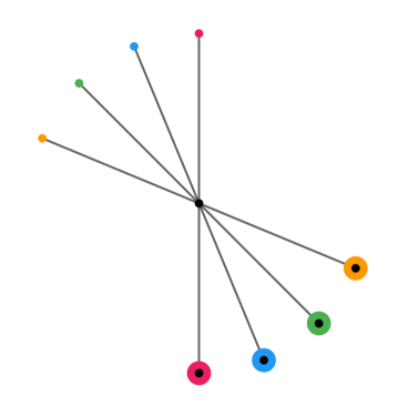
Figure 1: Bottleneck benchmark with $k=4$ agents.

The task here boils down to just choosing a certain order of the agents. Resolving such a benchmark problem can still result in an exponential complexity in the number of agents $k$—if just various permutations of the agents are tried, without a thorough exclusion of the conflicting time intervals of particular agents.

7.2 Experimental Setup

In the case of benchmarks empty and roadmap, we observe whether particular experiments finish within a given timeout. The set of experiments contains instances where the number of agents ranges from 1 to 64 (none of the tools managed to finish with more agents within the selected timeouts). For each number of agents $k\in\{1,\dots,64\}$, each start and goal vertex of each agent is pre-generated in 25 random variants. Here, when generating the variants for agent $k+1$, all the previous $k$ agents are reused and only the positions of the new one are generated randomly. The result is $64\times 25=1600$ instances for each of empty (for each neighborhood $n$) and roadmap.

The subject of our interest is how the evaluated algorithms scale with time, so we ran all the experiments with different timeouts ranging from 30 seconds up to 16 minutes (with exponential growth) and observed how many instances finished in time. We will show the results in the form of box plots.

To also directly illustrate the relationship of the number of solved instances and $k$, we will also show success rate plots, that is, plots with the ratios of the number of solved instances out of the total number of instances (i.e. out of 25) wrt. a given number of agents $k$, and with a fixed timeout.

Our tool SMT-LRA is in addition parametrized by a cost function—either makespan or sum of costs—and by a sub-optimal coefficient $\delta\in\{1,\frac{1}{2},\frac{1}{4}\}$. In the plots, the parameters are denoted in the form $(C,\delta)$, where $C$ is either M (makespan) or S (sum of costs). In all experiments, the higher $\delta$ was, the more instances were solved. Hence, to make the box plots more compact, we merged all the variants of $\delta$ related to the same cost function such that the boxes of the variants with lower $\delta$ overlay the boxes of the variants with higher $\delta$. Also, higher values of $\delta$ correspond to lighter colors. For example, boxes $\delta=\frac{1}{4}$ overlay boxes $\delta=\frac{1}{2}$, but the magnitudes of both boxes are still visible since the number of solved instances is always lower in the case of $\delta=\frac{1}{4}$ than in the case of $\delta=\frac{1}{2}$. As a result, for each timeout in the box plot, our tool always takes two columns, each consisting of three (overlaid) boxes. In the case of success rate plots, we use dashed curves in the case of our tool in order to increase readability, and include all curves that correspond to the variants of $\delta$, where again higher values of $\delta$ correspond to lighter colors.

We will provide tables to further illustrate the effect of parameter $\delta$. For this, observe that Algorithm 1 terminates as soon as $\mathit{cost}(p_{\mathit{opt}})\leq(1+\delta)t_{\mathit{min}}$, which ensures $\delta$-optimality. However, the ratio $\mathit{cost}(p_{\mathit{opt}})/t_{\mathit{min}}$, that we call guaranteed ratio, may actually be well below the required value $1+\delta$, meaning that the algorithm produced a better plan than required. The tables contain the average of the guaranteed ratio of plans that finished within 16 min (with lower timeouts, the ratios are even lower).

In the case of benchmark bottleneck, we only focus on runtime of the evaluated tools for some numbers of agents ranging from 2 to 30. In the case of our implementation, we again include all the variants of parameters mentioned above. We used timeout 30 min to set some upper boundary on the runtimes of the tools.

We executed all the benchmarks on a machine with Intel(R) Xeon(R) Gold 6254 CPU @ 3.10GHz, with 180 cores and 1TB memory. To unify the runtime environment, we reused and adapted the scripts from the previous experiments [1] which are a part of the SMT-CCBS tool. These scripts do not exploit all the available resources of the machine, though. Still, none of the evaluated tools use parallel computation—the cores are only used to run multiple benchmarks concurrently.

7.3 Results

Empty Room.

Recall that benchmark empty is parametrized by its neighborhood $n$ which means that vertices have approximately $2^{n}$ neighbors. We did experiments with $n\in\{2,3,4,5\}$, all of which are shown in box plots in Figure 2. We also provide Table 1 with guaranteed ratios of the resulting plans, depending on $n$.

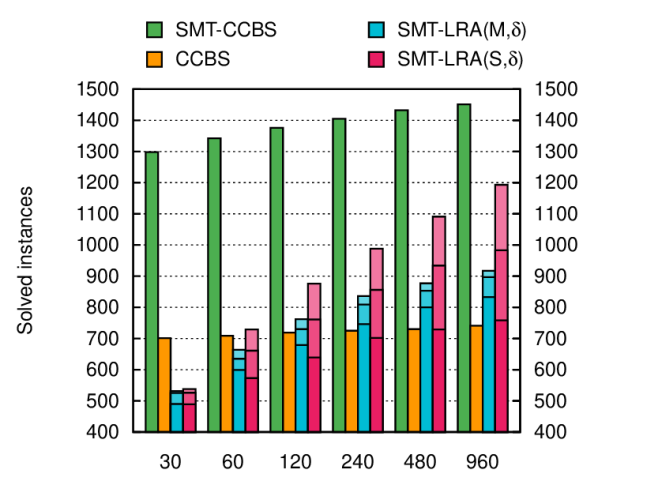
(a) $n=2$

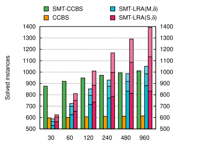
(b) $n=3$

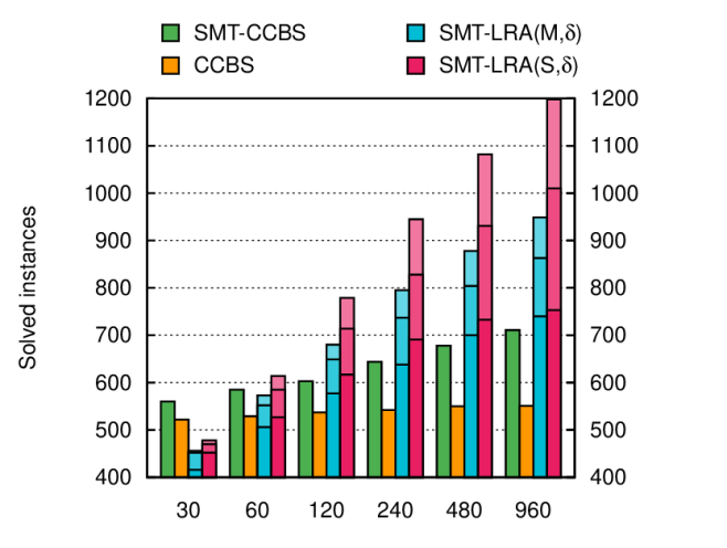
(c) $n=4$

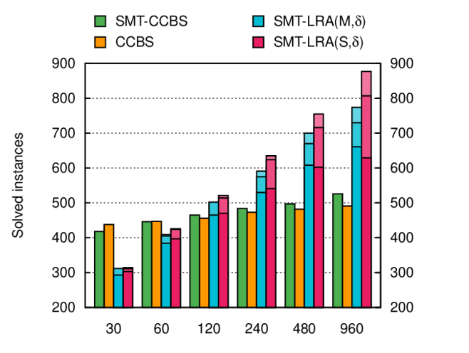
(d) $n=5$

Figure 2: Comparison of the number of solved instances of benchmark empty with given $n$ wrt. a given timeout.

Table 1: Average guaranteed ratios of SMT-LRA in benchmark empty wrt. the parameters of the tool and a given $n$.

$(C,\delta)\ \text{\textbackslash{}}\ n$	2	3	4	5
$(\texttt{M}{},1)$	1.45	1.55	1.54	1.43
$(\texttt{S}{},1)$	1.56	1.57	1.56	1.40
$(\texttt{M}{},0.5)$	1.29	1.33	1.32	1.29
$(\texttt{S}{},0.5)$	1.30	1.30	1.31	1.26
$(\texttt{M}{},0.25)$	1.16	1.18	1.18	1.17
$(\texttt{S}{},0.25)$	1.16	1.15	1.15	1.14

We firstly focus on the comparison of the selected cost functions in the case of our tool. We see that usually the cases that optimize sum of costs perform better than the cases optimizing makespan. Observe, though, that the results are similar in the case of $\delta=\frac{1}{4}$ which correspond to the boxes at the base. We explain these as that in the case of sum of costs there are more possibilities how to reduce the cost of the plan than in the case of makespan where the cost usually depends on just one agent, regarding the symmetry of the graph. We assume that at the same time this is the reason why, in the case of makespan, there are lower increases of the number of solved instances with growing $\delta$ compared to the variant which optimizes sum of costs. Also notice that in the cases of neighborhood $n=2$ and especially $n=5$, there are quite low performance growths with increasing $\delta$, which may be caused by the fact that the actual guaranteed ratio is lower than in other cases of $n$, namely with $\delta=1$ (see Table 1). Furthermore, [1] showed that these corner cases of $n$ are actually the least useful benchmarks: benchmarks with $n=3$ offer much faster plans than in the case of $n=2$, and $n=5$ on the other hand provide only very low improvement over the case of $n=4$. All in all, our approach scales well with the growing timeouts, in every case of neighborhood $n$, cost function and parameter $\delta$.

Now we also focus on the state-of-the-art tools, where we will actually confirm the observations made in [1]. These tools are consistent in the sense that the lower parameter $n$, the faster is their algorithm—because there are less possible paths to the goals. In our case, the observation holds as well, but with one exception in the case of $n=2$ vs. $n=3$, where the runtime of the experiments with the lowest neighborhood is higher. The reason is that the graphs with higher $n$ allow that the shortest paths to the goals take less edges—which in our case becomes more important than the number of possible choices, because our current algorithm is sensitive to the number of edges in the graph which we all encode into the formula.

The state-of-the-art tools usually perform better than our tool when the timeout is less or equal to 1 min. SMT-CCBS performs especially well in the case of $n=2$ because it maps a lot of time points to the same values since many of them are integer values. We however consider this case to be the least useful benchmark referring the earlier discussion and in addition since the square grids are not too realistic models and can also be handled by standard MAPF approaches (which are currently much faster than $\mathrm{MAPF}_{R}$ approaches). Although SMT-CCBS scales better with time than CCBS, the highest growth of the number of solved instances still occurs in the case of our approach, even in the cases of $\delta=\frac{1}{4}$ which correspond to the boxes of our algorithm at the base. In the cases of $n\geq 3$ and $\delta=1$, which correspond to the upmost boxes of our algorithm, we outperform the state-of-the-art tools if the timeout is high.

We also provide Figure 3 with success rate plots. Here we selected timeout 8 min (480 s). Recall that for our tool we distinguish the curves that correspond to higher $\delta$ by lighter colors. Within a single cost function, especially in the case of sum of costs, the distances between the curves of particular cases of $\delta$ seem to be quite uniform, which confirms the observations based on Figure 2 that in many cases our algorithm scales well with the parameter $\delta$. At the same time, the plots also confirm that sometimes in the case of makespan the performance does not increase much with growing $\delta$.

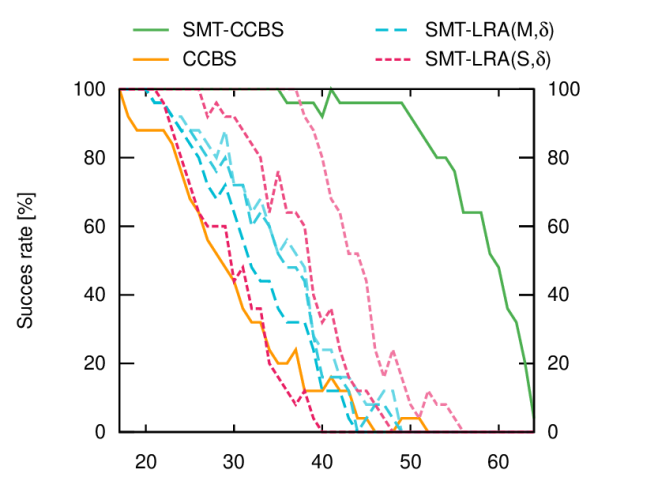
(a) $n=2$

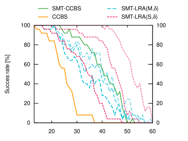
(b) $n=3$

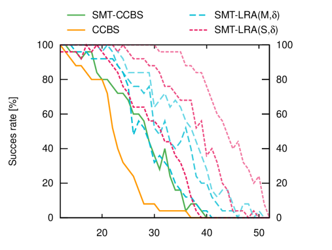
(c) $n=4$

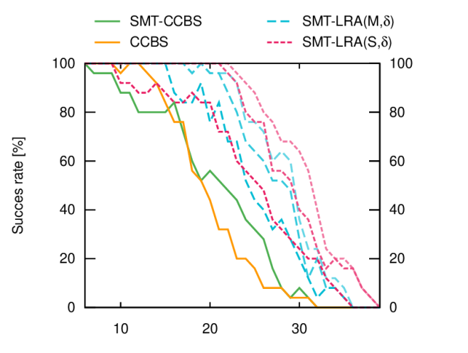
(d) $n=5$

Figure 3: Comparison of the success rates of benchmark empty with given $n$ within timeout 8 min wrt. a number of agents.

In the case of all the tools, especially in the case of our tool, there happen to be glitches in the success rates—sometimes the performance increases a bit with a higher number of agents. In some cases, it is probably just caused by inaccurate measurement, however approaches that are based on a SAT solver (SMT-CCBS) or even an SMT solver (SMT-LRA) may naturally exhibit such behavior since the algorithms are more complex and not that straightforward like CBS-based algorithms.

Roadmap.

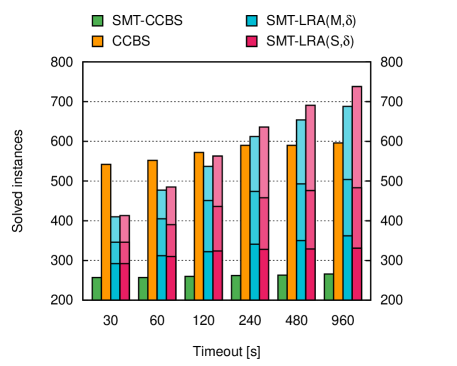
Figure 4: Comparison of the number of solved instances of benchmark roadmap wrt. a given timeout.

Figure 4 shows how particular tools scale with time in the case of benchmark roadmap. Clearly, SMT-CCBS does not handle this benchmark well, independent of the chosen timeout. By contrast, CCBS performs very well, especially with smaller timeouts. However, at the timeout of 4 min (240 s) it reaches a point after which it almost stops scaling with time at all. In our case, the variants which optimize sum of costs or makespan perform almost the same. However, the performance depends a lot on parameter $\delta$. For example, with $\delta=1$, which corresponds to the upmost boxes, our approach scales very well and outperforms CCBS for timeouts greater or equal to 4 min. However, in the cases of $\delta=\frac{1}{4}$ (i.e., the boxes at the base), the algorithm is not competitive with CCBS and scales poorly. We explain this as follows: the roadmap graph is highly asymmetric and contains a lot of long edges, compared to the graphs in benchmark empty. Therefore, the shortest paths to the goals often consist of a low number of edges. At the same time, paths to the goals with similar distances can actually consist of different number of edges. Thus, once we find a (collision-free) plan and fix the number of steps $h$ for all agents, it may happen that when optimizing the plan, we miss alternative paths that consist of more steps which could be essential to arriving at easier possibilities of finding faster plans.

In addition, we provide Table 2 with the guaranteed ratios of our tool. The ratios are quite high in the cases of $\delta=1$, which can explain why the difference of the number of solved instances is so high compared to $\delta=\frac{1}{2}$, and also compared to benchmark empty, where the guaranteed ratios are lower.

Table 2: Average guaranteed ratios of SMT-LRA in benchmark roadmap wrt. the parameters of the tool.

$(C,\delta)$
$(\texttt{M}{},1)$	1.64
$(\texttt{S}{},1)$	1.65
$(\texttt{M}{},0.5)$	1.31
$(\texttt{S}{},0.5)$	1.31
$(\texttt{M}{},0.25)$	1.14
$(\texttt{S}{},0.25)$	1.14

Similarly to benchmark empty, we also provide a plot with success rates of the tools, in Figure 5, again with the timeout of 8 min. Here the success rates are well distributed with no anomalies.

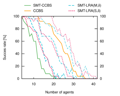
Figure 5: Comparison of the success rates of benchmark roadmap within timeout 8 min wrt. a number of agents.

Bottleneck.

We summarize the runtimes of benchmark bottleneck of particular tools in Table 3. In the case of SMT-CCBS, we excluded the built-in verification of the solutions which here seemed to be very time-consuming. In our case we merge all the corresponding cases of parameter $\delta$ into single column since the runtimes were almost the same regardless the parameter. We further merge both cost functions M and S into one column s.t. the respective runtimes are separated by a pipe character. The average guaranteed ratio of our presented plans is 1.08 in the case of makespan (M) and 1.04 in the case of sum of costs (S).

Table 3: Comparison of the runtimes in seconds of benchmark bottleneck with a given number of agents.

$k$	SMT-CCBS	CCBS	SMT-LRA$(\texttt{M}{}|\texttt{S}{}\!)$
2	0.00	0.00	0.01 $|$ 0.01
3	0.47	0.00	0.02 $|$ 0.02
4	$>1800$	0.00	0.04 $|$ 0.02
5	?	0.01	0.03 $|$ 0.03
6	?	0.05	0.07 $|$ 0.05
7	?	0.45	0.08 $|$ 0.06
8	?	3.52	0.15 $|$ 0.08
9	?	43.99	0.15 $|$ 0.11
10	?	720.27	0.22 $|$ 0.14
11	?	$>1800$	0.26 $|$ 0.17
15	?	?	0.46 $|$ 0.42
20	?	?	0.79 $|$ 0.97
30	?	?	4.88 $|$ 5.63

It is clear that runtimes of both state-of-the-art solvers exhibit exponential relationship with the number of agents $k$, while our algorithm is much less sensitive. For example, CCBS is fastest until $k=6$ but after that point our SMT-LRA dominates the runtime. The reason is that we resolve the conflicts of agents using the learning mechanism of generalized conflict clauses where the timing constraints efficiently exclude inappropriate orderings of the agents, making the benchmark fairly easy for our approach—which is consistent with the observation that such a problem is indeed trivial, as discussed in the description of benchmarks. For example, the problem is easily solvable using an ad-hoc approach. Nevertheless, such bottlenecks may appear as a part of more complex problems where a sophisticated algorithm instead of an ad-hoc should be used.

Profiling.

Profiling of our tool showed that the simulations used for collision detection and avoidance take a negligible part of the runtime. Instead, most of the time is spent in the SMT solver itself. If our approach was applied to benchmarks with large graphs (as discussed above), then also encoding the formula, conversion to CNF, etc., would take an additional important part of the runtime.

8 Conclusion

We have demonstrated how to solve the continuous-time MAPF problem ($\mathrm{MAPF}_{R}$) by direct translation to SAT modulo linear real arithmetic. While the approach insists only on sub-optimality up to a certain factor, it shows several advantages over state-of-the-art algorithms, especially better scaling wrt. an increasing time budget and its ability to efficiently handle bottleneck situations. Our approach also allows for easy change of the objective function to another. The downside is a certain basic translation effort, especially for problems depending on large graphs.

In future work we will explore a lazy approach to translation that only generates the information necessary for solving the current problem instance. This will be especially relevant in practical applications where similar problems have to be solved repeatedly. Moreover, we will generalize the method to problems with non-linear motion functions, allowing both non-linear geometry of the involved curves and the modeling of non-linear dynamical phenomena such as acceleration of agents. The method will also benefit from the fact that the efficiency of SMT solvers is currently improving with each year.

References

- [1] Anton Andreychuk, Konstantin S. Yakovlev, Pavel Surynek, Dor Atzmon, and Roni Stern. Multi-agent pathfinding with continuous time. Artif. Intell., 305:103662, 2022.
- [2] Dor Atzmon, Roni Stern, Ariel Felner, Nathan R. Sturtevant, and Sven Koenig. Probabilistic robust multi-agent path finding. In Proc. of the Thirtieth International Conference on Automated Planning and Scheduling, 2020, pages 29–37. AAAI Press, 2020.
- [3] Clark Barrett and Cesare Tinelli. Satisfiability modulo theories. In Edmund M. Clarke, Thomas A. Henzinger, Helmut Veith, and Roderick Bloem, editors, Handbook of Model Checking. Springer International Publishing, 2018.
- [4] Armin Biere. Bounded model checking. In Biere et al. [5].
- [5] Armin Biere, Marijn Heule, Hans van Maaren, and Toby Walsh, editors. Handbook of Satisfiability. IOS Press, 2nd edition, 2021.
- [6] Aysu Bogatarkan, Volkan Patoglu, and Esra Erdem. A declarative method for dynamic multi-agent path finding. In GCAI 2019. Proc. of the 5th Global Conference on Artificial Intelligence, volume 65 of EPiC Series in Computing, pages 54–67. EasyChair, 2019.
- [7] Michael Cashmore, Daniele Magazzeni, and Parisa Zehtabi. Planning for hybrid systems via satisfiability modulo theories. Journal of Artificial Intelligence Research, 67:235–283, 2020.
- [8] Alessandro Cimatti, Alberto Griggio, Bastiaan Schaafsma, and Roberto Sebastiani. The MathSAT5 SMT solver. In Nir Piterman and Scott Smolka, editors, Proc. of TACAS, volume 7795 of LNCS. Springer, 2013.
- [9] Liron Cohen, Tansel Uras, T. K. Satish Kumar, and Sven Koenig. Optimal and bounded-suboptimal multi-agent motion planning. In Proc. of the Twelfth International Symposium on Combinatorial Search, SOCS 2019, pages 44–51. AAAI Press, 2019.
- [10] Boris de Wilde, Adriaan ter Mors, and Cees Witteveen. Push and rotate: a complete multi-agent pathfinding algorithm. J. Artif. Intell. Res., 51:443–492, 2014.
- [11] Ariel Felner, Roni Stern, Solomon Eyal Shimony, Eli Boyarski, Meir Goldenberg, Guni Sharon, Nathan R. Sturtevant, Glenn Wagner, and Pavel Surynek. Search-based optimal solvers for the multi-agent pathfinding problem: Summary and challenges. In Proc. of the Tenth International Symposium on Combinatorial Search, SOCS 2017, pages 29–37. AAAI Press, 2017.
- [12] Graeme Gange, Daniel Harabor, and Peter J. Stuckey. Lazy CBS: implicit conflict-based search using lazy clause generation. In Proc. of the Twenty-Ninth International Conference on Automated Planning and Scheduling, ICAPS 2019, pages 155–162. AAAI Press, 2019.
- [13] Tomáš Kolárik and Stefan Ratschan. Railway scheduling using boolean satisfiability modulo simulations. In Marsha Chechik, Joost-Pieter Katoen, and Martin Leucker, editors, Formal Methods, number 14000 in LNCS, pages 56–73, Cham, 2023. Springer International Publishing.
- [14] Edward Lam, Pierre Le Bodic, Daniel Harabor, and Peter J. Stuckey. Branch-and-cut-and-price for multi-agent path finding. Comput. Oper. Res., 144:105809, 2022.
- [15] Francesco Leofante. Omtplan: a tool for optimal planning modulo theories. Journal on Satisfiability, Boolean Modeling and Computation, 14(1):17–23, 2023.
- [16] Jiaoyang Li, Zhe Chen, Daniel Harabor, Peter J. Stuckey, and Sven Koenig. Anytime multi-agent path finding via large neighborhood search. In Proc. of the Thirtieth International Joint Conference on Artificial Intelligence, IJCAI 2021, pages 4127–4135. ijcai.org, 2021.
- [17] Ryan Luna and Kostas E. Bekris. Push and swap: Fast cooperative path-finding with completeness guarantees. In IJCAI 2011, Proc. of the 22nd International Joint Conference on Artificial Intelligence, 2011, pages 294–300. IJCAI/AAAI, 2011.
- [18] Hang Ma. Intelligent planning for large-scale multi-agent systems. AI Mag., 43(4):376–382, 2022.
- [19] Jussi Rintanen. Planning and SAT. In Biere et al. [5].
- [20] Malcolm Ryan. Constraint-based multi-robot path planning. In IEEE International Conference on Robotics and Automation, ICRA 2010, pages 922–928. IEEE, 2010.
- [21] Malcolm R. K. Ryan. Exploiting subgraph structure in multi-robot path planning. J. Artif. Intell. Res., 31:497–542, 2008.
- [22] Guni Sharon, Roni Stern, Ariel Felner, and Nathan R. Sturtevant. Conflict-based search for optimal multi-agent pathfinding. Artif. Intell., 219:40–66, 2015.
- [23] David Silver. Cooperative pathfinding. In Proc. of the First Artificial Intelligence and Interactive Digital Entertainment Conference, 2005, pages 117–122. AAAI Press, 2005.
- [24] Pavel Surynek. Unifying search-based and compilation-based approaches to multi-agent path finding through satisfiability modulo theories. In Proc. of the Twenty-Eighth International Joint Conference on Artificial Intelligence, IJCAI 2019, pages 1177–1183. ijcai.org, 2019.
- [25] Pavel Surynek, Ariel Felner, Roni Stern, and Eli Boyarski. Efficient SAT approach to multi-agent path finding under the sum of costs objective. In ECAI 2016 - 22nd European Conference on Artificial Intelligence, volume 285 of Frontiers in Artificial Intelligence and Applications, pages 810–818. IOS Press, 2016.
- [26] Thayne T. Walker, Nathan R. Sturtevant, and Ariel Felner. Extended increasing cost tree search for non-unit cost domains. In Proc. of the Twenty-Seventh International Joint Conference on Artificial Intelligence, IJCAI 2018, pages 534–540. ijcai.org, 2018.