Electrodynamics and Geometric Continuum Mechanics
Abstract.
This paper offers an informal instructive introduction to some of the main notions of geometric continuum mechanics for the case of smooth fields. We use a metric invariant stress theory of continuum mechanics to formulate a simple generalization of the fields of electrodynamics and Maxwell’s equations to general differentiable manifolds of any dimension, thus viewing generalized electrodynamics as a special case of continuum mechanics. The basic kinematic variable is the potential, which is represented as a -form in an -dimensional spacetime. The stress for the case of generalized electrodynamics is assumed to be represented by an -form, a generalization of the Maxwell -form.
Key words and phrases:
Maxwell’s equations, pre-metric electrodynamics, -form electrodynamics, continuum mechanics, stress theory, differential forms.1. Introduction
This paper offers an informal instructive introduction to some of the main notions of geometric continuum mechanics for the case of smooth fields. Usually, continuum mechanics is thought of as the theoretical foundation for engineering stress analysis and fluid dynamics. Here, in order to motivate the constructions of geometric continuum mechanics, we show that the Maxwell equations of electromagnetism and generalizations thereof to metric-independent, or premetric, -form electrodynamics in an -dimensional spacetime may be obtained as a special case of geometric continuum mechanics. (See [HO03, Kai04, HIO06] for premetric electromagnetism and [HT86, HT88, NS12] for -form electrodynamics.) For the non-smooth counterpart of the theory, see [Seg16, Seg23].
The notations , and , are used for the electric displacement, electric field, magnetic field intensity, magnetic field flux density, current density, and charge density, respectively. Thus, the Maxwell equations are
| Gauss’s law, | (1.1) | ||||
| Gauss’s law for magnetism, | (1.2) | ||||
| Faraday’s law, | (1.3) | ||||
| Ampere’s law. | (1.4) |
Constitutive relations between the various fields should be added in order to make the system of equations solvable in principle.
We start by demonstrating in Section 2 how magnetostatics, for which the Maxwell equations assume a particularly simple form, may be obtained from the equation for the mechanical power in continuum mechanics for the generalized case where the stress tensor is antisymmetric, rather that symmetric.
Section 3 further motivates the usefulness of antisymmetric tensors by presenting the full set of Maxwell’s equation using antisymmetric tensors—differential forms—in a -dimensional spacetime devoid of metric properties. Then, some basic properties and operations corresponding to differential forms are briefly reviewed.
Next, starting with the classical definition, it is shown in Section 4 how the notion of a flux vector field can be generalized naturally and independently of a metric to the case of -dimensional manifolds by using differential -forms.
In Section 5, we consider the metric-invariant geometric theory of smooth force and stress fields in generalized media. In particular, a stress field is introduced as a tensor field that acts on generalized velocity fields to produce -forms that model the flux of power.
Finally, as our main example, we show in Section 6 that the generalization of Maxwell’s equations to -form, metric-independent electrodynamics in an -dimensional spacetime results from the basic properties of the stress under suitable assumptions. Specifically, it is assumed th at a generalized velocity is a -form, , in spacetime. Such a -form is interpreted as a generalized vector potential of electrodynamics. Next, it is assumed that the body force vanishes. Then, a particularly simple form for the stress is assumed. Namely, it is assumed that the stress is represented by an -form so that the action of the stress on the potential form is given as
| (1.5) |
where a wedge denotes the exterior product of differential forms.
It is noted that antisymmetric tensors were used in the formulation of electrodynamics by Truesdell and Toupin [TT60, Section F]. Whittaker [Whi53, pp. 192–196], attributes the first presentation of metric-free electrodynamics to Kottler [Kot22], while Truesdell and Toupin attribute the main contribution to van Dantzig [vD34].
For a comprehensive introduction to geometric continuum mechanics, which also includes a global non-smooth formulation, see [Seg23].
2. Magnetostatics and Generalized Media
When we specialize the Maxwell equations to the case of magnetostatics, we are concerned with the magnetic fields and in the case where all fields are time-independent. Thus, the resulting equations for magnetostatics are
| (2.1) |
Assuming that the physical space (at each instant) is simply connected, the equation implies that there is a (nonunique) vector field , the vector potential, such that
| (2.2) |
The identity , for every vector field , implies that the divergence of the vector field , as obtained from the vector potential, indeed vanishes.
Similarly, the equation implies that
| (2.3) |
—the conservation of charge. Conversely, conservation of charge implies that there is a vector potential such that . Thus, Equations (2.2,2.3) may be used alternatively to (2.1).
As a motivation for the more general construction, we show in this section that the equations of magnetostatics may be obtained as the equations of the mechanics of a generalized continuum.
We recall that given the body force, , and the surface force, , for the image in space of particular configuration of a material body, , the power expended for a virtual velocity , is given by
| (2.4) |
Consider the case whee , and use the basic property of the stress tensor as expressed by the Cauchy formula,
| (2.5) |
where is the Cauchy stress and is the unit normal to . The expression for the power assumes the form
| (2.6) |
Using the definition of the transpose of a linear mapping in a Euclidean space, and the expression for the power becomes
| (2.7) |
For classical continuum mechanics, the Cauchy stress tensor is symmetric so that the transposition is irrelevant. However, we may consider the case where the stress is an antisymmetric tensor. Clearly, this situation is outside the realm of classical continuum mechanics and belongs to the mechanics of generalized media. Thus, it is assumed henceforth that
| (2.8) |
Since is assumed to be antisymmetric, it may be represented by an axial vector , the components of which are given by
| (2.9) |
In terms of ,
| (2.10) |
and we can write for the power
| (2.11) |
Using the Gauss theorem,
| (2.12) |
We now make use of the identity
| (2.13) |
and obtaint
| (2.14) |
Anticipating the analogy with magnetostatics, we change the notation to to arrive at
| (2.15) |
Moreover, we may define
| (2.16) |
which implies immediately that
| (2.17) |
In terms of and , the expression for the power is
| (2.18) |
Evidently, we may now reinterpret as the vector potential, as the current density, as the magnetic field intensity, and as the magnetic flux density. In other words, if we admit antisymmetric stress tensors, which in the mechanical interpretation may be viewed as a smooth distribution of moments, mechanics has the same mathematical structure as magnetostatics.
It is noted that, for continuum mechanics, the power may also be written as
| (2.19) |
where the summation convention is used, and a comma denotes partial differentiation. Thus, for the case of an antisymmetric stress tensor, only the antisymmetric, spin part , of the velocity gradient is relevant. This was expected as we consider a generalized continuum for which the kinematics is not represented merely by the velocity of the material points in space.
3. Manifolds and Differential Forms
It is observed that the field equations for magnetostatics, as presented above, look simpler and more symmetric than the full set of Maxwell’s equations. However, in an appropriate -dimensional setting, the Maxwell equations attain the same simplicity and symmetry as the equations for magnetostatics. In fact, they are completely analogous.
In addition to the simplicity, the version of the Maxwell equations we write below, does not use any metric properties of the ambient medium, be it the physical space or a body of continuum mechanics. Thus, as geometrical objects, the electromagnetic fields in a body are independent of deformations of the body in space. In addition, this may be relevant for general relativity, where the metric tensor is unknown a priori.
The Faraday -tensor and the Maxwell -tensor are defined, respectively, by
| (3.1) |
In addition, consider the vector
| (3.2) |
i.e., , , etc., and define the antisymmetric -tensor by
| (3.3) |
Similarly to the equations of magnetostatics, the Maxwell equations may be written now in the form
| (3.4) |
where d denotes a differential operator to be described below. If the potential -tensor is defined by
| (3.5) |
where is the electrostatic potential, then, the analogs of Equations (2.2,2.3) are, respectively,
| (3.6) |
Now that we have demonstrated the power provided by making use of antisymmetric tensors, we will shortly and roughly review the main definitions and results. For details, see [Seg23] or the comprehensive [AMR88, Lee02].
Differentiable manifolds are characterized by the property that points on them can be identified using local coordinate systems, or charts, with points in . Transformations of coordinates are smooth and reversible to make the assignment of coordinates consistent. Smooth curves are well-defined on a manifold. A tangent vector at a point may be defined as the derivative of a smooth curve passing through that point with respect to the curve parameter, and one writes
| (3.7) |
where is the curve.
An example of a differentiable manifold is the configuration space modeling the kinematics of a mechanical system having a finite number of degrees of freedom. Another example is a body of continuum mechanics for which a natural reference configuration is not given. For this example, viewing a tangent vector as an infinitesimal vector adjoining two neighboring points, it is evident that two tangent vectors at distinct points cannot be compared, added, etc. as objects should be invariant under any superimposed deformation. If denotes a differentiable manifold, the collection of tangent vectors at an arbitrary point , denoted by , may be given the structure of a vector space. In general, no inner product structure is given on .
At each point, one can consider completely antisymmetric -tensors, scalar-valued -multilinear mappings of tangent vectors at this point. Such a tensor field, assigning an antisymmetric tensor on for each , is a differential -form. Thus, the electromagnetic fields introduced above are differential forms. For example, the field is a differential -form on the -dimensional spacetime.
Any tensor , in general not antisymmetric, induces an antisymmetric tensor . The components of may be obtained from the components of using the alternating symbol. The operation is a projection in the sense that an antisymmetric tensor is invariant under its action.
Remark 3.1.
Note that the components , , , of any completely antisymmetric -tensor in an -dimensional space are determined by the components , , , with the properties that . It follows that the dimension of the space of antisymmetric -tensors in an -dimensional space is
| (3.8) |
the number of possible ways to choose numbers from . In particular,
| (3.9) |
The exterior product of an -form and a -form , is the form defined by
| (3.10) |
Thus, in essence, the exterior product is the antisymmetrized tensor product. In fact, the exterior product generalizes the “cross” product of vectors in a -dimensional Euclidean space to any pair of tensors in any dimension of the ambient space without using an inner product.
The exterior derivative, , of a differential -form, , can roughly by described as the antisymmetrized gradient of the differential form. It is an -form that has the following properties.
For a -form, a real valued function defined on the manifold, the -form is defined by
| (3.11) |
where . It follows that is the directional derivative of the function in the direction of .
The second property of exterior differentiation is that
| (3.12) |
Roughly, as the second derivative is symmetric its antisymmetrization naturally vanishes. This property generalizes classical identities of vector analysis, such as and .
Finally, for an -form and a -form ,
| (3.13) |
which generalizes the Leibniz rule.
These three properties are sufficient to define the exterior derivative uniquely as a linear differential operator. In terms of components, the exterior derivative may be expressed as the exterior product of the operator with the representative of .
As mentioned above, for a function, a -form, the exterior derivative is analogous to the gradient. The exterior derivative of a -form is analogous to the curl of a vector field. The exterior derivative of a -form in a -dimensional manifold, or in general, the exterior derivative of an -form in an -dimensional manifold, is analogous to the divergence of a vector field.
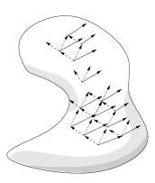
Differential forms are natural integrands on manifolds. The integral of an -form over an -dimensional manifold may be described roughly as follows. Divide the manifold into infinitesimal parallelepipeds, each of which is determined by a collection of tangent vectors. Here, because of the antisymmetry of the differential form to be integrated, one has to make sure that the collections of vectors at the various points are ordered consistently. Then, add up the actions of the differential form on the collections of vectors determining the parallelepipeds at the various points (see a rough illustration in Figure 3.1).
The integration of the -form, , over the -dimensional manifold, , is denoted as
| (3.14) |
Using the language of differential forms and their integration, the classical Green theorem, Gauss theorem, and Kelvin-Stokes theorem, may be generalized to one compact form. Specifically, the geometric Stokes theorem states that for an -form , the integral over the boundary of an -dimensional manifold , satisfies
| (3.15) |
Note that is an -dimensional manifold and is an -form, so that the integrals above are meaningful. The theorem is based on the fundamental theorem of calculus.
4. The Representation of Fluxes by Differential Forms
The notion of a flux vector field, such as the heat flux vector field, or the momentum flux vector field, is fundamental in continuum mechanics. We will denote a generic flux vector field of classical continuum mechanics by . If is a surface in a -dimensional Euclidean with unit normal vector field , the flux through , in the sense determined by , is given by
| (4.1) |
The infinitesimal version is evidently
| (4.2) |
where is the infinitesimal area vector so that .
Consider the case where the infinitesimal area vector is determined by two infinitesimal vectors and originating from a point on the surface so that
| (4.3) |
Then, the infinitesimal flux through the area element is given by
| (4.4) |
We now view as the evaluation of a function of the two vectors and write this as
| (4.5) |
By its definition and the properties of the “cross” product, is linear in each of the vectors and is antisymmetric. It is concluded that is an antisymmetric -tensor and assuming it varies smoothly with , there is a -form such that
| (4.6) |
It is emphasized that while the classical expression for the flux as in Equation (4.1) depends on the availability of the scalar product, the expressions in Equation (4.6) in terms of differential forms are independent of any scalar product and remain invariant under deformations of .
In general, one can use the integration of an -form on an -dimensional submanifold as a generalization of the standard flux in three dimensions. In most cases, . For example, the spacetime of classical mechanics is a -dimensional manifold without a natural scalar product. Integration of forms enables one to compute fluxes of -forms through -dimensional submanifolds of spacetime and also the fluxes of -forms through -dimensional submanifolds.
5. Forces and Traction Stresses on Manifolds
We have already emphasized that tangent vectors at distinct points in a manifold cannot be compared, added, etc. As a consequence, the same applies to tensors acting on vectors. It follows that it is meaningless to integrate force vectors over a body in the setting of a manifold. As noted above, natural integrands on an -dimensional manifolds are -forms, which we interpret as densities of some scalar extensive properties.
For the case of forces, the density to be integrated is that of the mechanical power expended by a force field for a given velocity field. Consequently, the notion of mechanical power assumes a major role in the formulation of metric-invariant force and stress theory.
Consider, for example, body forces in continuum mechanics. For an infinitesimal volume element , the power expended by the body force for the velocity is
| (5.1) |
Let be three linearly independent infinitesimal vectors that generate a parallelepiped with volume , so,
| (5.2) |
Thus,
| (5.3) |
We wish to view as a function of the vectors so
| (5.4) |
The properties of the determinant imply immediately that is an antisymmetric -tensor and so, assuming that it varies smoothly with , is a -form. In addition, depends linearly on .
Hence, the body force at the point is a linear mapping acting on values of velocity fields to produce antisymmetric -tensors. The body force field is a tensor field that when acting on a velocity field, it yields a -form . It is observed that the definition extends naturally to the case of a generalized medium, where is any generalized velocity field. This definition does not require any metric property of space and the body force field, so defined, is invariant under deformations of the body. This definition also generalizes naturally to any dimension by replacing above with a generic . The total power of the body force acting on a region is given, therefore, as an integral of the resulting -form by
| (5.5) |
Analogous arguments imply that the surface force, acting on the boundary , is a tensor field that acts on generalized velocity fields, , to produce an -forms, , defined on , and the power expended is
| (5.6) |
It is emphasized that for , is an antisymmetric tensor acting on vectors that are tangent to at .
The considerations corresponding to the stress object combine those related to fluxes with those related to forces. For standard continuum mechanics, the Cauchy stress , at a point in the body, determines the surface force on any subbody , the boundary of which contains , using the Cauchy formula
| (5.7) |
where is the unit normal to at .
Let be an infinitesimal area element on at . Then the infinitesimal power flux through for a velocity is
| (5.8) |
Using the definition of the transpose of a linear mapping,
| (5.9) |
so,
| (5.10) |
For standard continuum mechanics, the stress tensor is symmetric so that transposition has no consequences. However, anticipating the extension to generalized media, we keep the indication of a transposition.
Let be two infinitesimal vectors tangent to at that induce a parallelogram tangent to of area
| (5.11) |
Then, the power is given as
| (5.12) |
As before, we wish to view the power as the evaluation of a function on the vectors . That is,
| (5.13) |
It is emphasized that in this expression the vectors are viewed as vectors in the body and need not be tangent to the boundary of a particular body, in contrast with the case of a surface force on a particular subbody. Once the two vectors are given, the power of the surface force , for any subbody the tangent plane to the boundary of which contains these vectors, is induced.
Comparing the last equation with the discussion in Section 4, it follows that
| (5.14) |
is a -form in the body that depends linearly on the values of .
It is concluded that the stress object is a tensor field that, when acting on a velocity field it produces a power flux -form in the body. It is noted again that the antisymmetric -tensor acts on any pair of vectors at , and is not restricted, as is, to vectors tangent to the boundary of a particular subbody. In fact, the analog of the Cauchy formula is simply the restriction of the tensor to vectors tangent to .
The extension to generalized media in dimensions is straightforward. The stress is a tensor field that acts on generalized velocity fields to produce -forms. Given such a stress , the power of the surface force induced by the stress on a subbody is given by
| (5.15) |
The Stokes theorem implies immediately the power may also be written as
| (5.16) |
6. Maxwell’s Equations and -Form Electrodynamics
Finally, we show how metric-independent, -form electrodynamics in an -dimensional spacetime results as a special case of geometric stress theory as described above. To that end, we make the following assumptions.
Assumption I
Generalized velocity fields are -forms in -dimensional spacetime.
A -form representing a generalized velocity is interpreted as a potential for the electromagnetic fields. This interpretation will be justified below. In order to reflect this interpretation, we will change the notation for a generic generalized velocity form to .
It is recalled that the value of the stress at a point is a linear mapping that acts on a generalized velocity—now, an antisymmetric -tensor—to yield an antisymmetric -tensor representing the flux of power. In light of Remark 3.1, the dimension of the space of antisymmetric -tensors is
| (6.1) |
and that corresponding to antisymmetric -tensors is . Hence, the dimension of the space of values of the stress tensor at a point is
| (6.2) |
Assumption II
The body force vanishes, that is, .
As a result of this assumption, the total power for a given generalized velocity is
| (6.3) |
The most significant assumption is
Assumption III
There is an -form, , such that the power flux -form, , is given by
| (6.4) |
It is noted first that the degrees of the forms and indeed add up to . It is also noted that this assumption imposes a significant restriction on the stress. The dimension of the space of values of antisymmetric -tensors is
| (6.5) |
in comparison with the dimension for the general case given by Equation (6.2).
It follows from this assumption that the power is given by
| (6.6) |
We may now use the rule for the differentiation of the exterior product, (3.13), to obtain
| (6.7) |
Setting,
| (6.8) |
the expression for the power assumes the form
| (6.9) |
Finally, it follows immediately from the definitions in (6.8) and property (3.12) of differential forms that
| (6.10) |
Acknowledgments. This work was partially supported by the Pearlstone Center for Aeronautical Engineering Studies at Ben-Gurion University.
References
- [AMR88] R. Abraham, J.E. Marsden, and T. Ratiu. Manifolds, Tensor Analysis. and Applications. Springer, 1988.
- [HIO06] F.W. Hehl, Y. Itin, and Y.N. Obukhov. Recent developments in premetric electrodynamics. arXiv:physics/0610221v1 [physics.class-ph], October 2006.
- [HO03] F.W. Hehl and W.N. Obukhov. Foundations of Classical Electrodynamics: Charge, Flus, and Metric. Birkhauser, 2003.
- [HT86] M. Henneaux and C. Teitelboim. -form electrodynamics. Foundations of Physics, 16(7):593–617, 1986.
- [HT88] M. Henneaux and C. Teitelboim. Dynamics of chiral (self-dual) -forms. Physics Letters B, 206:650–654, 1988.
- [Kai04] G. Kaiser. Energy-momentum conservation in pre-metric electrodynamics with magnetic charges. Journal of Physics A: Mathematical and General, 37:7163–7168, 2004.
- [Kot22] F. Kottler. Maxwell’sche gleichungen und metrik. Sitzungsberichte Akademie der Wissenschaften in Wien (IIa), 131:119–146, 1922.
- [Lee02] J.M. Lee. Introduction to Smooth Manifolds. Springer-Verlag, 2002.
- [NS12] J. Navarro and J.B. Sancho. Energy and electromagnetism of a differential -form. Journal of Mathematical Physics, 53:102501, 2012.
- [Seg16] R. Segev. Continuum mechanics, stresses, currents and electrodynamics. Philosophical Transactions of the Royal Society of London A, 374:20150174, 2016. DOI: 10.1098/rsta.2015.0174.
- [Seg23] R. Segev. Foundations of Geometric Continuum Mechanics. 2023. Forthcoming.
- [TT60] C.A. Truesdell and R. Toupin. The Classical Field Theories, volume III/1 of Handbuch der Physik. Springer, 1960.
- [vD34] D. van Dantzig. The fundamental equations of electromagnetism, independent of metrical geometry. Proceedings of the Cambridge Philosophical Society, 30:421–427, 1934.
- [Whi53] E.T. Whittaker. A History of the Theories of Aether and Electricity, volume 2. Nelson, 1953.