Convergence analysis of Hermite approximations for analytic functions

Abstract

In this paper, we present a rigorous analysis of root-exponential convergence of Hermite approximations, including projection and interpolation methods, for functions that are analytic in an infinite strip containing the real axis and satisfy certain restrictions on the asymptotic behavior at infinity within this strip. Asymptotically sharp error bounds in the weighted and maximum norms are derived. The key ingredients of our analysis are some remarkable contour integral representations for the Hermite coefficients and the remainder of Hermite spectral interpolations. Further extensions to Gauss–Hermite quadrature, Hermite spectral differentiations, generalized Hermite spectral approximations and the scaling factor of Hermite approximation are also discussed. Numerical experiments confirm our theoretical results.

Keywords: Hermite spectral approximations, analytic functions, root-exponential convergence, contour integral representations, Gauss–Hermite quadrature

AMS classifications: 41A25, 41A10

1 Introduction

Hermite polynomials/functions are orthogonal systems on the real line, which serve as a natural choice of basis functions when dealing with practical problems on infinite intervals. Hermite spectral methods, which are achieved by Hermite spectral approximations including expansions or interpolations via Hermite polynomials/functions, play an important role in solving PDEs in unbounded domains (cf. [4, 5, 22]). Several attractive advantages of Hermite spectral methods can be summarized as follows:

• Hermite functions are the eigenfunctions or the limiting asymptotic eigenfunctions of many problems of physical interests [3].

• Hermite differentiation matrix is skew-symmetric, tridiagonal and irreducible, which leads to conservative semidiscretisations for time-dependent PDEs [14]. Moreover, the spectral radii for the first and second Hermite differentiation matrices are $O(\sqrt{n})$ and $O(n)$, respectively, where $n$ is the number of terms of Hermite spectral approximation. This particularly implies rather weak stability restrictions on the time step when explicit time stepping methods are applied to the semidiscretisation system [35].

A fundamental issue toward understanding the convergence behavior of Hermite spectral methods is to establish rigorous error analysis of Hermite spectral approximations. When the underlying function is analytic, Hille in [12, 13] and Szegő in [24] established the domain of convergence for the Hermite expansions in the complex plane. More precisely, Hille in [12, 13] proved that the domain is an infinite strip when the underlying function is analytic and decays exponentially at infinity within this strip. The situation is much more delicate for entire functions in the sense that the convergence domain of Hermite expansions depends on its growth order as well. Elliott and Tuan in [10] established a contour integral representation for the Hermite coefficients. Unfortunately, no further analysis on the decay rate of Hermite coefficients or the convergence rate of Hermite expansions was carried out. Based on Hille’s works, Boyd in [2, 3] refined the connection between the asymptotic estimate of Hermite coefficients and the behavior of the underlying functions at infinity. In particular, asymptotic results of Hermite coefficients for some specific entire functions (namely, super- and sub-Gaussian types) and analytic functions with poles were obtained by using the method of steepest descent. Although these studies provide important insights onto the convergence properties of Hermite approximations, a number of essential issues still remain open. For example, no sharp error bounds were studied for Hermite expansions of analytic functions and, as far as we know, no discussion was devoted to the analysis of exponential convergence of Hermite spectral interpolations.

It is the aim of this work to present a rigorous convergence analysis of Hermite spectral approximations, including Hermite projection and interpolation methods, for analytic functions. When the underlying function is analytic in an infinite strip containing the real axis and satisfies some restrictions on the asymptotic behavior at infinity within this strip, we establish contour integral representations for the Hermite coefficients and the remainder of Hermite spectral interpolations over the boundary of the infinite strip. These, together with asymptotic behaviors of Hermite polynomials as well as their weighted Cauchy transforms, allow us to establish some asymptotically sharp error bounds for Hermite projection and interpolation methods. Extensions of our analysis to some related topics, including Gauss-Hermite quadrature, Hermite spectral differentiations, generalized Hermite spectral approximations and the scaling factor of Hermite approximation, are also discussed.

It is worthwhile to point out that rigorous convergence analysis of spectral approximations of analytic functions have attracted renewed interests over the past few decades; cf. [20, 29, 30, 31, 32, 33, 36, 37, 38, 39]. However, most of these studies were devoted to Jacobi approximations as well as the special cases like Chebyshev, Legendre and Gegenbauer approximations. Compared with Jacobi case, the convergence analysis of Laguerre and Hermite cases is much more difficult since their convergence rates depend not only on the locations of the singularities, but also on the asymptotic behavior of the underlying function at infinity. More recently, by exploiting contour integral techniques, the first-named author established some sharp error estimates for Laguerre projection and interpolation methods in [32]. Here we extend the idea therein to Hermite case and our analysis relies heavily on some remarkable contour integral representations for Hermite coefficients and the remainder of Hermite spectral interpolations. These integrals involve Hermite polynomials and their weighted Cauchy transforms, which might be of independent interests.

The rest of this paper is organized as follows. In the next section, we collect some properties of Hermite polynomials and the associated weighted Cauchy transforms. In Sections 3 and 4, we prove the root-exponential convergence of Hermite projections and interpolations for analytic functions, respectively. We extend our analysis to several topics of practical interests in Section 5 and present some concluding remarks in Section 6.

2 Hermite polynomials and their weighted Cauchy transforms

In this section, we review some basic facts of Hermite polynomials and establish some new properties of their weighted Cauchy transforms. For more information about Hermite polynomials, we refer to [19, 24] and the references therein.

Let $\omega(x)=e^{-x^{2}}$ be the Hermite weight function and let $\mathbb{N}_{0}:=\{0,1,2,\ldots\}$. For each $n\in\mathbb{N}_{0}$, we denote by $H_{n}(x)$ the Hermite polynomial of degree $n$, which is defined by

$$H_{n}(x)=\frac{(-1)^{n}}{\omega(x)}\frac{\mathrm{d}^{n}\omega(x)}{\mathrm{d}x^{n}}.$$ (2.1)

It is well-known that Hermite polynomials satisfy the orthogonality condition

$$\langle H_{n},H_{m}\rangle_{\omega}=\gamma_{n}\delta_{n,m},\quad\gamma_{n}=2^{n}n!\sqrt{\pi},$$ (2.2)

where $n,m\in\mathbb{N}_{0}$ and

$$\langle f,g\rangle_{\omega}:=\int_{-\infty}^{\infty}f(x)g(x)\omega(x)\mathrm{d}x$$ (2.3)

is the weighted inner product over the real axis and $\delta_{n,m}$ stands for the Kronecker delta. More properties of Hermite polynomials are listed below.

• The three term recurrence relation of $H_{n}$ reads

  $$H_{n+1}(x)=2xH_{n}(x)-2nH_{n-1}(x),\quad n\in\mathbb{N},$$ (2.4)

  $$H_{0}(x)=1,\quad H_{1}(x)=2x.$$

• By [19, Equation (18.14.9)], we have

  $$e^{-x^{2}/2}|H_{n}(x)|\leq\frac{\sqrt{\gamma_{n}}}{\pi^{1/4}},\qquad x\in\mathbb{R},$$ (2.5)

  where $\gamma_{n}$ is given in (2.2). By [24, Theorem 8.22.7], we have

  $$|e^{-z^{2}/2}H_{n}(z)|=\frac{\Gamma(n+1)}{2\Gamma(n/2+1)}e^{|\Im(z)|\sqrt{2n+1}}\left(1+O(n^{-1/2})\right),\quad\Im(z)\neq 0,$$ (2.6)

  where $\Gamma(z)$ is the gamma function.

• Since $\omega(x)=\omega(-x)$, it follows that

  $$H_{n}(-x)=(-1)^{n}H_{n}(x).$$ (2.7)

We then define the weighted Cauchy transform of Hermite polynomials by

$$\Phi_{n}(z)=\frac{1}{2\pi\mathrm{i}}\int_{\mathbb{R}}\frac{\omega(x)H_{n}(x)}{z-x}\mathrm{d}x,\quad z\in\mathbb{C}\setminus\mathbb{R},$$ (2.8)

where $\mathrm{i}$ is the imaginary unit. In the literature [15, 24], the function $\Phi_{n}(z)/\omega(z)$ is also known as the function of the second kind associated with Hermite polynomials (up to the prefactor). It is easily seen that $\Phi_{n}(z)$ is analytic in the whole complex plane with a cut along $\mathbb{R}$, and satisfies the same recurrence relation as $H_{n}$ given in (2.4). We establish some important properties of $\Phi_{n}(z)$ in what follows for later use.

Lemma 2.1.

The function $\Phi_{n}$ defined in (2.8) satisfies the following properties.

• For any $x\in\mathbb{R}$, we have

  $$\begin{cases}{\displaystyle\lim_{\varepsilon\rightarrow 0+}\left[\Phi_{n}(x-\mathrm{i}\varepsilon)+\Phi_{n}(x+\mathrm{i}\varepsilon)\right]=\frac{1}{\pi\mathrm{i}}\mathchoice{{\vbox{\hbox{$\textstyle-$}}\kern-4.86108pt}}{{\vbox{\hbox{$\scriptstyle-$}}\kern-3.25pt}}{{\vbox{\hbox{$\scriptscriptstyle-$}}\kern-2.29166pt}}{{\vbox{\hbox{$\scriptscriptstyle-$}}\kern-1.875pt}}\!\int_{\mathbb{R}}\frac{\omega(y)H_{n}(y)}{x-y}\mathrm{d}y},\\[12.91663pt] {\displaystyle\lim_{\varepsilon\rightarrow 0+}\left[\Phi_{n}(x-\mathrm{i}\varepsilon)-\Phi_{n}(x+\mathrm{i}\varepsilon)\right]=\omega(x)H_{n}(x)},\end{cases}$$ (2.9)

  where the bar indicates the Cauchy principal value.

• As $z\rightarrow\infty$, we have

  $$\Phi_{n}(z)=\frac{n!}{2\sqrt{\pi}\mathrm{i}z^{n+1}}+O(z^{-n-2}).$$ (2.10)

• Let $U(a,b;z)$ be the confluent hypergeometric function of the second kind (also known as Kummer’s function of the second kind, cf. [19, Chapter 13]), we have

  $$\Phi_{n}(z)=\frac{\Gamma(n+1)}{2\sqrt{\pi}}U\left(\frac{n+1}{2},\frac{1}{2},-z^{2}\right)\left\{\begin{array}[]{ll}{\displaystyle e^{-(n+2)\pi\mathrm{i}/2}},&\Im(z)>0,\\[10.0pt] {\displaystyle e^{n\pi\mathrm{i}/2}},&\Im(z)<0.\end{array}\right.$$ (2.11)

• As $n\rightarrow\infty$, we have

  $$|\Phi_{n}(z)| =\frac{\Gamma(n+1)|e^{-z^{2}/2}|}{\Gamma(\frac{n+1}{2})\sqrt{2(n+1)}}e^{-|\Im(z)|\sqrt{2(n+1)}}\left(1+O(n^{-1/2})\right).$$ (2.12)

Proof.

The first statement is a direct consequence of the Plemelj formula [18]. For the second statement, by expanding $1/(z-x)$ in (2.8) as

$$\frac{1}{z-x}=\sum_{k=0}^{n}\frac{x^{k}}{z^{k+1}}+\frac{x^{n+1}}{(z-x)z^{n+1}},$$

and using the orthogonality condition (2.2) of Hermite polynomials, it is readily seen that

$$\Phi_{n}(z)=\frac{1}{2\pi\mathrm{i}z^{n+1}}\int_{\mathbb{R}}x^{n}H_{n}(x)\omega(x)\mathrm{d}x+O(z^{-n-2})=\frac{n!}{2\sqrt{\pi}\mathrm{i}z^{n+1}}+O(z^{-n-2}),$$

where we have used the fact that the leading coefficient of $H_{n}(x)$ is $2^{n}$ in the last step. This proves (2.10). Alternatively, assuming (2.11), it also follows from the fact (cf. [19, Equation (13.7.3)]) that as $z\to\infty$,

$$U(a,b;z)\sim z^{-a},\qquad|\arg(z)|<\frac{3\pi}{2}.$$

For the third statement, by the integral representation of Hermite polynomials given in [19, Equation (18.10.10)] and exchanging the order of integration, we have

$$\Phi_{n}(z) =\frac{2^{n+1}}{2\pi\mathrm{i}\sqrt{\pi}}\int_{0}^{\infty}e^{-t^{2}}t^{n}\left(\int_{\mathbb{R}}\frac{\cos(2xt-n\pi/2)}{z-x}\mathrm{d}x\right)\mathrm{d}t$$

$$=\frac{2^{n}}{\sqrt{\pi}}\left\{\begin{array}[]{ll}{\displaystyle e^{-(n+2)\pi\mathrm{i}/2}\int_{0}^{\infty}e^{-t^{2}+2\mathrm{i}zt}t^{n}\mathrm{d}t},&\Im(z)>0,\\[8.61108pt] {\displaystyle e^{n\pi\mathrm{i}/2}\int_{0}^{\infty}e^{-t^{2}-2\mathrm{i}zt}t^{n}\mathrm{d}t},&\Im(z)<0,\end{array}\right.$$ (2.15)

$$=\frac{2^{n/2}\Gamma(n+1)e^{-z^{2}/2}}{\sqrt{2\pi}}\left\{\begin{array}[]{ll}{\displaystyle e^{-(n+2)\pi\mathrm{i}/2}U(n+1/2,-\mathrm{i}\sqrt{2}z)},&\Im(z)>0,\\[8.61108pt] {\displaystyle e^{n\pi\mathrm{i}/2}U(n+1/2,\mathrm{i}\sqrt{2}z)},&\Im(z)<0,\end{array}\right.$$ (2.18)

where $U(a,z)$ is the Weber parabolic cylinder function [19, Equation (12.5.1)]. Here, the second equality in the above equation follows from the facts that

$$\int_{\mathbb{R}}\frac{e^{\mathrm{i}\lambda x}}{z-x}\mathrm{d}x=\left\{\begin{array}[]{ll}{\displaystyle-2\pi\mathrm{i}e^{\mathrm{i}\lambda z}},&\Im(z)>0,\\[8.61108pt] {\displaystyle 0},&\Im(z)<0,\end{array}\right.\quad\int_{\mathbb{R}}\frac{e^{-\mathrm{i}\lambda x}}{z-x}\mathrm{d}x=\left\{\begin{array}[]{ll}{\displaystyle 0},&\Im(z)>0,\\[8.61108pt] {\displaystyle 2\pi\mathrm{i}e^{\mathrm{i}\lambda z}},&\Im(z)<0,\end{array}\right.$$

for $\lambda>0$, which can be obtained by the residue theorem and Jordan’s lemma. Combining the last equation of (2) with [19, Equation (12.7.14)] gives (2.11). Finally, to show the estimate (2.12), we observe from [27, Equations (2.6), (2.11) and (2.14)] and [26, Remark 10.2] that as $a\to+\infty$,

$$U(a,b;z)=\frac{2}{\Gamma(a)}\left(\frac{z}{a}\right)^{(1-b)/2}e^{z/2}K_{b-1}(2\sqrt{az})\left(1+O(a^{-1/2})\right),$$ (2.19)

for $z\in\mathbb{C}\setminus(-\infty,0]$, where $K_{\nu}$ is the modified Bessel function of the second kind. On account of the fact (cf. [19, Equation (10.40.2)]) that as $z\to\infty$,

$$K_{\nu}(z)=\sqrt{\frac{\pi}{2z}}e^{-z}\left(1+O(z^{-1})\right),\qquad|\arg z|<\frac{3\pi}{2},$$

it is readily seen that

$$U(a,b;z)=\frac{\sqrt{\pi}}{\Gamma(a)}\left(\frac{z}{a}\right)^{(1-b)/2}\frac{\exp(z/2-2\sqrt{az})}{(az)^{1/4}}\left(1+O(a^{-1/2})\right),\quad a\to+\infty,$$ (2.20)

for $z\in\mathbb{C}\setminus(-\infty,0]$. A combination of (2.11) and the above asymptotic estimate gives us (2.12). This completes the proof of Lemma 2.1. ∎

3 Convergence analysis of Hermite projections

In this section, we carry out a thorough convergence analysis of Hermite projections. To proceed, we introduce an infinite strip in the complex plane

$$\mathcal{S}_{\rho}:=\big{\{}z\in\mathbb{C}:~{}\Im(z)\in[-\rho,\rho]\big{\}},$$ (3.1)

where $\rho>0$, and denote by $\partial{\mathcal{S}}_{\rho}$ the boundary of $\mathcal{S}_{\rho}$; see Figure 1 for an illustration. The domain of convergence of a Hermite series is actually characterized by $\mathcal{S}_{\rho}$, where the parameter $\rho$ is determined by the location of the singularities and the asymptotic behavior at infinity of the underlying function; see [12, 13].

Figure 1: The infinite strip $\mathcal{S}_{\rho}$ and its boundary.

3.1 Projections using Hermite polynomials

Let $\mathbb{P}_{n}$ be the space of polynomials of degree up to $n$ and denote by $L_{\omega}^{2}(\mathbb{R})$ the Hilbert space consisting of all squared integrable functions with respect to the Hermite weight function $\omega(x)$ over $\mathbb{R}$, equipped with the inner product (2.3) and the norm

$$||f||_{L_{\omega}^{2}(\mathbb{R})}=\sqrt{\langle f,f\rangle}_{\omega}.$$ (3.2)

We set $\Pi_{n}^{\mathrm{P}}:L_{\omega}^{2}(\mathbb{R})\rightarrow\mathbb{P}_{n}$ to be the orthogonal projection operator, i.e., for any $f\in{L}_{\omega}^{2}(\mathbb{R})$,

$$(\Pi_{n}^{\mathrm{P}}f)(x)=\sum_{k=0}^{n}a_{k}H_{k}(x),\qquad a_{k}=\frac{\langle f,H_{k}\rangle_{\omega}}{\gamma_{k}},$$ (3.3)

where $H_{k}$ is the Hermite polynomial of degree $k$. The following theorem shows that the coefficient $a_{n}$ admits a contour integral representation involving the weighted Cauchy transform of the Hermite polynomial $H_{n}$, which plays an important role in our further analysis. In what follows, the orientation of a closed curve in the complex plane is always taken in a counterclockwise manner.

Theorem 3.1.

If $f$ is analytic in the infinite strip $\mathcal{S}_{\rho}$ for some $\rho>0$ and $|f(z)|\leq\mathcal{K}|z|^{\sigma}$ for some $\sigma\in\mathbb{R}$ as $|z|\rightarrow\infty$ within the strip, it then holds that, for each $n\geq\max\{\lfloor\sigma\rfloor,0\}$,

$$a_{n}=\frac{1}{\gamma_{n}}\int_{\partial{\mathcal{S}}_{\rho}}\Phi_{n}(z)f(z)\mathrm{d}z,$$ (3.4)

where $\Phi_{n}$ is defined in (2.8).

Proof.

Let $\varepsilon$ and $\eta$ be two arbitrary positive constants, we set the following auxiliary contours:

$$\Gamma_{\pm}^{\mathrm{D}}:~{}~{}z =x\pm\mathrm{i}\varepsilon,\quad\Gamma_{\pm}^{\mathrm{U}}:~{}~{}z=x\pm\mathrm{i}\rho,\qquad x\in[-\eta,\eta],$$ (3.5)

$$\Gamma_{\pm}^{\mathrm{R}}:~{}~{}z =\eta\pm\mathrm{i}y,\quad\Gamma_{\pm}^{\mathrm{L}}:~{}~{}z=-\eta\pm\mathrm{i}y,\qquad y\in[\varepsilon,\rho];$$

see Figure 2 for an illustration and the orientations.

Since $\Phi_{n}(z)$ is analytic in the whole complex plane except the real line, it follows from Cauchy’s theorem that

$$\int_{\Gamma_{+}^{\mathrm{D}}\cup\Gamma_{-}^{\mathrm{D}}\cup\Gamma_{-}^{\mathrm{R}}\cup\Gamma_{+}^{\mathrm{R}}\cup\Gamma_{+}^{\mathrm{U}}\cup\Gamma_{-}^{\mathrm{U}}\cup\Gamma_{+}^{\mathrm{L}}\cup\Gamma_{-}^{\mathrm{L}}}\Phi_{n}(z)f(z)\mathrm{d}z =0.$$ (3.6)

Figure 2: The contours $\Gamma_{\pm}^{\mathrm{D}},\Gamma_{\pm}^{\mathrm{U}},\Gamma_{\pm}^{\mathrm{R}}$ and $\Gamma_{\pm}^{\mathrm{L}}$ defined in (3.5).

We next evaluate the integrals over different contours as $\varepsilon\rightarrow 0^{+}$ and $\eta\to\infty$. By (2.9), we note that

$$\lim_{\begin{subarray}{c}\varepsilon\rightarrow 0^{+}\\ \eta\rightarrow\infty\end{subarray}}\int_{\Gamma_{-}^{\mathrm{U}}\cup\Gamma_{+}^{\mathrm{D}}}\Phi_{n}(z)f(z)\mathrm{d}z =-\lim_{\begin{subarray}{c}\varepsilon\rightarrow 0^{+}\\ \eta\rightarrow\infty\end{subarray}}\int_{-\eta}^{\eta}(\Phi_{n}(x-\mathrm{i}\varepsilon)-\Phi_{n}(x+\mathrm{i}\varepsilon))f(x)\mathrm{d}x$$

$$=-\int_{\mathbb{R}}\omega(x)H_{n}(x)f(x)\mathrm{d}x$$

$$=-\gamma_{n}a_{n},$$

where we have made use of the definition of $a_{n}$ in (3.3). For the contour integrals over $\Gamma_{-}^{\mathrm{R}}\cup\Gamma_{+}^{\mathrm{R}}$ and $\Gamma_{+}^{\mathrm{L}}\cup\Gamma_{-}^{\mathrm{L}}$, by item (ii) of Lemma 2.1 and the condition that $|f(z)|\leq\mathcal{K}|z|^{\sigma}$ with $\sigma<n+1$ for large $z$, we obtain that

$$\lim_{\begin{subarray}{c}\varepsilon\rightarrow 0^{+}\\ \eta\rightarrow\infty\end{subarray}}\int_{\Gamma_{-}^{\mathrm{R}}\cup\Gamma_{+}^{\mathrm{R}}}\Phi_{n}(z)f(z)\mathrm{d}z =\mathrm{i}\lim_{\eta\rightarrow\infty}\int_{-\rho}^{\rho}\Phi_{n}(\eta+\mathrm{i}y)f(\eta+\mathrm{i}y)\mathrm{d}y=0,$$

and similarly,

$$\lim_{\begin{subarray}{c}\varepsilon\rightarrow 0^{+}\\ \eta\rightarrow\infty\end{subarray}}\int_{\Gamma_{+}^{\mathrm{L}}\cup\Gamma_{-}^{\mathrm{L}}}\Phi_{n}(z)f(z)\mathrm{d}z =(-\mathrm{i})\lim_{\eta\rightarrow\infty}\int_{-\rho}^{\rho}\Phi_{n}(-\eta+\mathrm{i}y)f(-\eta+\mathrm{i}y)\mathrm{d}y=0.$$

Finally, it is easily seen that

$$\lim_{\eta\rightarrow\infty}\int_{\Gamma_{+}^{\mathrm{U}}\cup\Gamma_{-}^{\mathrm{U}}}\Phi_{n}(z)f(z)\mathrm{d}z =\int_{\partial\mathcal{S}_{\rho}}\Phi_{n}(z)f(z)\mathrm{d}z.$$

By taking $\varepsilon\rightarrow 0^{+}$ and $\eta\to\infty$ on both sides of (3.6), we arrive at (3.4) with the aid of the above four formulas. This ends the proof of Theorem 3.1. ∎

Remark 3.2.

It is easily seen that (3.4) holds for all $n\geq 0$ when $|f(z)|\leq\mathcal{K}|z|^{\sigma}$ for some $\sigma<1$.

Remark 3.3.

It is possible to derive the exact formula of the Hermite coefficients for functions with poles in the complex plane. For example, for $f(x)=1/(x^{2}+\tau^{2})$ with $\tau>0$, by combining Theorem 3.1 and the residue theorem, we obtain that

$$a_{n}=\frac{\cos(n\pi/2)}{2^{n}\tau}U\left(\frac{n+1}{2},\frac{1}{2},\tau^{2}\right),\quad n\in\mathbb{N}_{0}.$$ (3.7)

As a consequence of the above theorem, we are able to establish the root-exponential convergence of Hermite projections in the weighted $L^{2}$-norm for analytic functions.

Theorem 3.4.

If $f$ satisfies the assumptions of Theorem 3.1 and set

$$V:=\int_{\partial\mathcal{S}_{\rho}}|e^{-z^{2}/2}f(z)|\mathrm{d}z.$$ (3.8)

The following statements hold.

• For each $n\geq\max\{\lfloor\sigma\rfloor,0\}$, the Hermite coefficients $a_{n}$ satisfy

  $$|a_{n}|\leq\frac{\mathcal{K}e^{-\rho\sqrt{2(n+1)}}}{2^{n}\sqrt{2\pi(n+1)}\Gamma(\frac{n+1}{2})},$$ (3.9)

  where $\mathcal{K}\approx V$ for $n\gg 1$.

• The error of Hermite projection in the weighted $L^{2}$-norm satisfies

  $$\|f-\Pi_{n}^{\mathrm{P}}f\|_{L_{\omega}^{2}(\mathbb{R})}\leq\mathcal{K}e^{-\rho\sqrt{2n}},$$ (3.10)

  where $\mathcal{K}\approx V/\sqrt{4\pi\rho}$ for $n\gg 1$.

Proof.

We obtain from Theorem 3.1, (2.12) and (2.2) that

$$|a_{n}| \leq\frac{1}{\gamma_{n}}\int_{\partial\mathcal{S}_{\rho}}|\Phi_{n}(z)f(z)|\mathrm{d}s\leq\frac{e^{-\rho\sqrt{2(n+1)}}}{2^{n}\Gamma(\frac{n+1}{2})\sqrt{2\pi(n+1)}}\left(V+O(n^{-1/2})\right),$$

and therefore (3.9) follows immediately.

To show (3.10), it is readily seen from (3.9) that

$$\|f-\Pi_{n}^{\mathrm{P}}f\|_{L_{\omega}^{2}(\mathbb{R})}^{2} =\sum_{k=n+1}^{\infty}a_{k}^{2}\gamma_{k}\leq\frac{\mathcal{K}^{2}}{\sqrt{\pi}}\sum_{k=n+1}^{\infty}\frac{e^{-2\rho\sqrt{2(k+1)}}\Gamma(k+1)}{2^{k+1}(k+1)\Gamma(\frac{k+1}{2})^{2}},$$ (3.11)

where $\mathcal{K}\approx V$ for $n\gg 1$. From the duplication formula and ratio asymptotics for the gamma function (see [19, Equations (5.5.5) and (5.11.13)]), it follows that

$$\frac{\Gamma(k+1)}{2^{k+1}(k+1)\Gamma(\frac{k+1}{2})^{2}} =\frac{\Gamma(\frac{k}{2}+1)}{2\sqrt{\pi}(k+1)\Gamma(\frac{k+1}{2})}\leq\frac{\mathcal{K}}{2\sqrt{2\pi(k+1)}},$$ (3.12)

where $\mathcal{K}\approx 1$ for $n\gg 1$. This, together with (3.11), implies that

$$\|f-\Pi_{n}^{\mathrm{P}}f\|_{\omega}^{2} \leq\frac{\mathcal{K}^{2}}{2\pi}\sum_{k=n+1}^{\infty}\frac{e^{-2\rho\sqrt{2(k+1)}}}{\sqrt{2(k+1)}}$$

with $\mathcal{K}\approx V$ for $n\gg 1$. Since

$$\sum_{k=n+1}^{\infty}\frac{e^{-2\rho\sqrt{2(k+1)}}}{\sqrt{2(k+1)}}\leq\int_{n+1}^{\infty}\frac{e^{-2\rho\sqrt{2x}}}{\sqrt{2x}}\mathrm{d}x=\frac{e^{-2\rho\sqrt{2(n+1)}}}{2\rho},$$

the desired result (3.10) follows. This completes the proof of Theorem 3.4. ∎

Remark 3.5.

When $\max_{z\in\partial\mathcal{S}_{\rho}}|f(z)|$ is bounded, the quantity $V$ can be bounded by

$$V \leq\int_{\partial\mathcal{S}_{\rho}}|e^{-z^{2}/2}|\mathrm{d}z\max_{z\in\partial\mathcal{S}_{\rho}}|f(z)|=2\sqrt{2\pi}e^{\rho^{2}/2}\max_{z\in\partial\mathcal{S}_{\rho}}|f(z)|.$$

Figure 3: The magnitudes of the Hermite coefficients $\{a_{n}\}$ (dots) of $f(x)=1/(1+25x^{2}),~{}e^{-x^{2}}/(4+x^{2}),~{}\mathrm{sech}(\pi x/8)$ (from the top to the bottom) as a function of $n$. The dashed lines show the predicted rates with $\rho=1/5,~{}2,~{}4$, respectively.

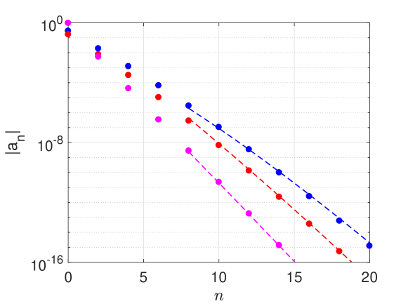
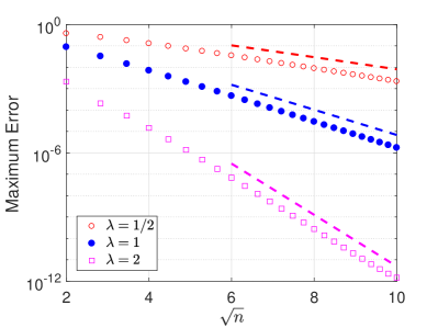
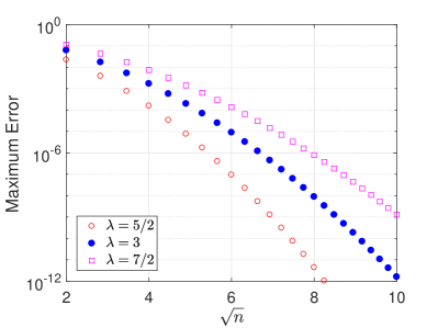
From Theorem 3.4, it follows that the Hermite coefficients $\{a_{n}\}$ in (3.3) decay at a super-exponential rate for analytic functions. In Figure 3, we plot the magnitudes of the Hermite coefficients of the following three analytic functions

$$f(x)=\frac{1}{1+25x^{2}},\qquad\frac{e^{-x^{2}}}{x^{2}+4},\qquad\mathrm{sech}\left(\frac{\pi x}{8}\right).$$

It is easy to check that they all satisfy the assumptions of Theorem 3.4, and they are analytic in the infinite strip $\mathcal{S}_{\rho}$ with $\rho=1/5-\epsilon,~{}2-\epsilon,~{}4-\epsilon$, respectively, where $\epsilon>0$ is arbitrarily close to zero. Note that we only plot the magnitudes of the Hermite coefficients $\{a_{n}\}$ with even $n$ since $a_{n}=0$ for odd $n$. From Figure 3 we can see that the actual decay rates of the Hermite coefficients of these three functions are consistent with our predictions.

3.2 Projections using Hermite functions

The Hermite functions are defined by

$$\psi_{n}(x)=\frac{e^{-x^{2}/2}H_{n}(x)}{\sqrt{\gamma_{n}}},\qquad n\in\mathbb{N}_{0},$$ (3.13)

which are preferable in practice. By (2.2), it is easily seen that $\{\psi_{n}\}_{n=0}^{\infty}$ are orthonormal with respect to the usual inner product, i.e.,

$$\int_{\mathbb{R}}\psi_{n}(x)\psi_{m}(x)\mathrm{d}x=\delta_{n,m},\qquad n,m\in\mathbb{N}_{0},$$ (3.14)

and, by (2.5),

$$|\psi_{n}(x)|\leq\frac{1}{\pi^{1/4}},\qquad n\in\mathbb{N}_{0},\quad x\in\mathbb{R}.$$ (3.15)

An appealing property of Hermite functions is that they are eigenfunctions of the Fourier transform [19, Equation (18.17.22)]. Specifically, we have

$$\psi_{n}(x)=\frac{\mathrm{i}^{-n}}{\sqrt{2\pi}}\int_{\mathbb{R}}e^{\mathrm{i}xy}\psi_{n}(y)\mathrm{d}y.$$

Indeed, this property serves as a key ingredient to develop Hermite spectral methods for PDEs involving a fractional Laplacian operator [17].

We now introduce the space $\mathbb{H}_{n}=\mathrm{span}\{\psi_{k}\}_{k=0}^{n}$, which is spanned by Hermite functions, and let $\Pi_{n}^{\mathrm{F}}:L^{2}(\mathbb{R})\rightarrow\mathbb{H}_{n}$ be the orthogonal projection operator from $L^{2}(\mathbb{R})$ upon $\mathbb{H}_{n}$. For any $f\in{L}^{2}(\mathbb{R})$, its orthogonal projection upon $\mathbb{H}_{n}$ reads

$$(\Pi_{n}^{\mathrm{F}}f)(x)=\sum_{k=0}^{n}c_{k}\psi_{k}(x),\qquad c_{k}=\int_{\mathbb{R}}f(x)\psi_{k}(x)\mathrm{d}x.$$ (3.16)

Let $\|\cdot\|_{L^{2}(\mathbb{R})}$ and $\|\cdot\|_{L^{\infty}(\mathbb{R})}$ stand for the norms induced by the usual inner product and by the maximum norm over $\mathbb{R}$, respectively. Below we give error estimates for orthogonal projection based on Hermite functions both in the $L^{2}$-norm and in the $L^{\infty}$-norm.

Theorem 3.6.

Let $f$ be analytic in the infinite strip $\mathcal{S}_{\rho}$ for some $\rho>0$ and $|e^{z^{2}/2}f(z)|\leq\mathcal{K}|z|^{\sigma}$ for some $\sigma\in\mathbb{R}$ as $|z|\to\infty$ within the strip. Set

$$\widehat{V}:=\int_{\partial\mathcal{S}_{\rho}}|f(z)|\mathrm{d}z.$$ (3.17)

The following statements hold.

• For each $n\geq\max\{\lfloor\sigma\rfloor,0\}$, the Hermite coefficient in (3.16) satisfies

  $$|c_{n}|\leq\mathcal{K}\frac{e^{-\rho\sqrt{2(n+1)}}}{(n+1)^{1/4}},$$ (3.18)

  where $\mathcal{K}\approx\widehat{V}/(2^{3/4}\sqrt{\pi})$ for $n\gg 1$.

• The error of Hermite projection in the $L^{2}$-norm satisfies

  $$\|f-\Pi_{n}^{\mathrm{F}}f\|_{L^{2}(\mathbb{R})}\leq\mathcal{K}e^{-\rho\sqrt{2n}},$$ (3.19)

  where $\mathcal{K}\approx\widehat{V}/\sqrt{4\pi\rho}$ for $n\gg 1$.

• The error of Hermite projection in the $L^{\infty}$-norm satisfies

  $$\|f-\Pi_{n}^{\mathrm{F}}f\|_{L^{\infty}(\mathbb{R})}\leq\mathcal{K}n^{1/4}e^{-\rho\sqrt{2n}},$$ (3.20)

  where $\mathcal{K}\approx\widehat{V}/(2^{1/4}\pi^{3/4}\rho)$ for $n\gg 1$.

Proof.

Note that the $n$-th coefficient $c_{n}$ in terms of Hermite functions is exactly the $n$-th coefficient of $e^{x^{2}/2}f(x)\sqrt{\gamma_{n}}$ in terms of Hermite polynomials, it follows from Theorem 3.4 that

$$|c_{n}| \leq\frac{\mathcal{K}\sqrt{\gamma_{n}}e^{-\rho\sqrt{2(n+1)}}}{2^{n}\sqrt{2\pi(n+1)}\Gamma(\frac{n+1}{2})},$$

where $\mathcal{K}\approx\widehat{V}$ for $n\gg 1$. Furthermore, using the duplication formula and ratio asymptotics for the gamma function (see [19, Equations (5.5.5) and (5.11.13)]), one finds

$$\frac{\sqrt{\gamma_{n}}}{2^{n}\sqrt{2\pi(n+1)}\Gamma(\frac{n+1}{2})} =\frac{1}{\sqrt{2\pi(n+1)}}\sqrt{\frac{\Gamma(\frac{n+2}{2})}{\Gamma(\frac{n+1}{2})}}\leq\frac{\mathcal{K}}{2^{3/4}\sqrt{\pi}(n+1)^{1/4}},$$

where $\mathcal{K}\approx 1$ for $n\gg 1$. Combining the above two results gives (3.18). As for (3.19), by (3.14) and (3.18), we have

$$\|f-\Pi_{n}^{\mathrm{F}}f\|_{L^{2}(\mathbb{R})}^{2} =\sum_{k=n+1}^{\infty}(c_{k})^{2}\leq\mathcal{K}^{2}\sum_{k=n+1}^{\infty}\frac{e^{-2\rho\sqrt{2(k+1)}}}{\sqrt{k+1}},$$ (3.21)

where $\mathcal{K}\approx\widehat{V}/(2^{3/4}\sqrt{\pi})$ for $n\gg 1$. Note that

$$\sum_{k=n+1}^{\infty}\frac{e^{-2\rho\sqrt{2(k+1)}}}{\sqrt{k+1}}\leq\int_{n+1}^{\infty}\frac{e^{-2\rho\sqrt{2x}}}{\sqrt{x}}\mathrm{d}x=\frac{e^{-2\rho\sqrt{2(n+1)}}}{\sqrt{2}\rho}.$$

The estimate (3.19) follows by inserting the above inequality into (3.21).

To show (3.20), we see from the inequalities (3.15) and (3.18) that

$$\|f-\Pi_{n}^{\mathrm{F}}f\|_{L^{\infty}(\mathbb{R})} \leq\frac{1}{\pi^{1/4}}\sum_{k=n+1}^{\infty}|c_{k}|\leq\frac{\mathcal{K}}{\pi^{1/4}}\sum_{k=n+1}^{\infty}\frac{e^{-\rho\sqrt{2(k+1)}}}{(k+1)^{1/4}},$$

where $\mathcal{K}\approx\widehat{V}/(2^{3/4}\sqrt{\pi})$ for $n\gg 1$. For the summation in the last inequality, we note that

$$\sum_{k=n+1}^{\infty}\frac{e^{-\rho\sqrt{2(k+1)}}}{(k+1)^{1/4}}\leq\int_{n+1}^{\infty}\frac{e^{-\rho\sqrt{2x}}}{x^{1/4}}\mathrm{d}x=\frac{2^{1/4}}{\rho^{3/2}}\Gamma\left(\frac{3}{2},\rho\sqrt{2(n+1)}\right),$$

where $\Gamma(a,z)$ is the incomplete gamma function. The estimate (3.20) follows by combining the fact that $\Gamma(a,z)=z^{a-1}e^{-z}(1+O(z^{-1}))$ as $z\to\infty$ (see [19, Equation (8.11.2)]) with the above two inequalities. This completes the proof of Theorem 3.6. ∎

Figure 4: Maximum error of the Hermite projection $\Pi_{n}^{\mathrm{F}}f$ as a function of $\sqrt{n}$ for $f(x)=e^{-x^{2}}/(x^{2}+2)$ (left) and $f(x)=e^{-x^{2}/2}\sin(3x)/\sqrt{x^{2}+2}$ (right). The dashed lines show $O(n^{1/4}\exp(-2\sqrt{n}))$.

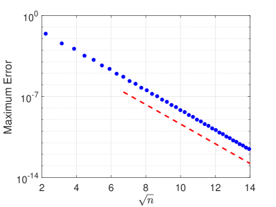
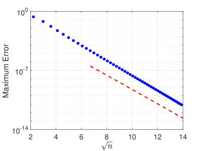
In Figure 4 we plot the maximum error of the Hermite projection $\Pi_{n}^{\mathrm{F}}f$ for $f(x)=e^{-x^{2}}/(x^{2}+2)$ and $f(x)=e^{-x^{2}/2}\sin(3x)/\sqrt{x^{2}+2}$. Clearly, both functions have pole and branch point singularities, respectively, at $\pm\sqrt{2}\mathrm{i}$ and they are analytic in the infinite strip $\mathcal{S}_{\rho}$ with $\rho=\sqrt{2}-\epsilon$, where $\epsilon>0$ is arbitrarily close to zero. We conclude from (3.20) that the predicted rate of convergence of $\Pi_{n}^{\mathrm{F}}f$ in the $L^{\infty}$-norm is $O(n^{1/4}e^{-2\sqrt{n}})$ as $n\rightarrow\infty$. From Figure 4 we can see that the actual rates of convergence of $\Pi_{n}^{\mathrm{F}}f$ are consistent with the predicted ones.

Remark 3.7.

Hille in [12, 13] showed that $|c_{n}|=O(\exp(-\rho\sqrt{2n}))$ if $f$ is analytic in the strip $\mathcal{S}_{\rho}$ and $|f(z)|\leq B(\rho)\exp(-|\Re(z)|\sqrt{\rho^{2}-\Im(z)^{2}})$ for $z\in\mathcal{S}_{\rho}$ and $B(\rho)$ is some finite positive constant. Boyd in [3] further analyzed the function $f(x)=e^{-x^{2}}/(x^{2}+\rho^{2})$ and showed that its Hermite coefficients satisfy $|c_{n}|\sim 2^{5/4}\sqrt{\pi}Rn^{-1/4}\exp(-\rho\sqrt{2n})$ as $n\rightarrow\infty$, where $R$ is the residue of $f$ at the poles $z=\pm\mathrm{i}\rho$. Note that our result in Theorem 3.6 contains the prefactor $n^{-1/4}$, which is more precise than Hille’s result, but with a stronger assumption on the asymptotic behavior of the underlying function at infinity. Moreover, our result is more general than Boyd’s result in the sense that it has no restriction on the types of singularities.

4 Convergence analysis of Hermite spectral interpolations

In this section, we are concerned with convergence rate of Hermite spectral interpolations for analytic functions. Let $\{x_{k}\}_{k=0}^{n}$ be the zeros of $H_{n+1}(x)$ and we assume that they are arranged in ascending order, i.e., $-\infty<x_{0}<x_{1}<\cdots<x_{n}<\infty$. By the symmetry relation (2.7) of Hermite polynomials, it is easily seen that $x_{k}=-x_{n-k}$ for $k=0,\ldots,n$. Let $p_{n}$ be the unique polynomial of degree $n$ which interpolates $f(x)$ at the points $\{x_{k}\}_{k=0}^{n}$, i.e.,

$$p_{n}(x_{j})=f(x_{j}),\quad j=0,\ldots,n.$$ (4.1)

which is also known as the Hermite spectral interpolation. The proof of root-exponential convergence of $p_{n}$ will be the main topic of this section.

We start with presenting a contour integral representation of the remainder for Hermite spectral interpolations by extending the idea of [32, Lemma 4.1].

Lemma 4.1.

Under the same assumptions of Theorem 3.1, for $x\in\mathbb{R}$ and $n\geq\max\{\lfloor\sigma\rfloor,0\}$, we have

$$f(x)-p_{n}(x)=\frac{1}{2\pi\mathrm{i}}\int_{\partial{\mathcal{S}}_{\rho}}\frac{H_{n+1}(x)f(z)}{H_{n+1}(z)(z-x)}\mathrm{d}z,$$ (4.2)

where $p_{n}$ is the polynomial of degree $n$ determined through (4.1).

Proof.

Let $\eta>0$ be large enough such that $x\in(-\eta,\eta)$ and set

$$V_{\pm}:~{}~{}z=\pm\eta+\mathrm{i}y,\qquad y\in[-\rho,\rho].$$

Note that $V_{\pm}$ are related to the contours $\Gamma_{\pm}^{\mathrm{R}}$ and $\Gamma_{\pm}^{\mathrm{L}}$ defined in (3.5) by $V_{+}=\Gamma_{+}^{\mathrm{R}}\cup\Gamma_{-}^{\mathrm{R}}$ and $V_{-}=\Gamma_{+}^{\mathrm{L}}\cup\Gamma_{-}^{\mathrm{L}}$ with $\varepsilon=0$. By Hermite’s contour integral [6, Theorem 3.6.1], the remainder of $p_{n}(x)$ can be written as

$$f(x)-p_{n}(x)=\frac{1}{2\pi\mathrm{i}}\int_{\Gamma_{-}^{\mathrm{U}}\cup\Gamma_{+}^{\mathrm{U}}\cup V_{+}\cup V_{-}}\frac{H_{n+1}(x)f(z)}{H_{n+1}(z)(z-x)}\mathrm{d}z.$$ (4.3)

For $z\in{V}_{+}$, we have

$$\left|\int_{V_{+}}\frac{H_{n+1}(x)f(z)}{H_{n+1}(z)(z-x)}\mathrm{d}z\right|\leq\left|\frac{H_{n+1}(x)}{H_{n+1}(\eta)}\right|\int_{V_{+}}\frac{|f(z)|}{|z-x|}\mathrm{d}s\leq 2\rho\cdot\left|\frac{H_{n+1}(x)}{H_{n+1}(\eta)}\right|\max_{z\in{V_{+}}}\left|\frac{f(z)}{z-x}\right|,$$

and similarly,

$$\left|\int_{V_{-}}\frac{H_{n+1}(x)f(z)}{H_{n+1}(z)(z-x)}\mathrm{d}z\right|\leq\left|\frac{H_{n+1}(x)}{H_{n+1}(\eta)}\right|\int_{V_{-}}\frac{|f(z)|}{|z-x|}\mathrm{d}s\leq 2\rho\cdot\left|\frac{H_{n+1}(x)}{H_{n+1}(\eta)}\right|\max_{z\in{V_{-}}}\left|\frac{f(z)}{z-x}\right|.$$

Clearly, we see that the above two bounds behave like $O(\eta^{\sigma-n-2})$ as $\eta\rightarrow\infty$. Since $n\geq\max\{\lfloor\sigma\rfloor,0\}$, it is easily seen that

$$\sigma-n\left\{\begin{array}[]{ll}<1,&\hbox{$\sigma>0$,}\\[4.30554pt] \leq 0,&\hbox{$\sigma=0$,}\\[4.30554pt] \leq\sigma,&\hbox{$\sigma<0$.}\end{array}\right.$$

Thus, by taking $\eta\rightarrow\infty$ on both sides of (4.3) and noting that $\partial{\mathcal{S}}_{\rho}=\Gamma_{-}^{\mathrm{U}}\cup\Gamma_{+}^{\mathrm{U}}$, we obtain the desired result from the above three estimates. This completes the proof of Lemma 4.1. ∎

As a consequence, we could establish the following root-exponential convergence of Hermite spectral interpolation in the weighted $L^{2}$-norm.

Theorem 4.2.

Under the conditions of Lemma 4.1, for $n\geq\max\{\lfloor\sigma\rfloor,0\}$, we have

$$\|f-p_{n}\|_{L_{\omega}^{2}(\mathbb{R})}\leq\mathcal{K}n^{1/4}e^{-\rho\sqrt{2n}},$$ (4.4)

where $\mathcal{K}\approx V/(2^{1/4}\rho\sqrt{\pi})$ for $n\gg 1$ with $V$ given in (3.8).

Proof.

By (3.2) and Lemma 4.1, it follows that

$$\|f-p_{n}\|_{L_{\omega}^{2}(\mathbb{R})}^{2} =\int_{\mathbb{R}}\omega(x)(f(x)-p_{n}(x))^{2}\mathrm{d}x\leq\frac{\gamma_{n+1}}{4(\pi\rho)^{2}}\left(\int_{\partial{\mathcal{S}}_{\rho}}\frac{|f(z)|}{|H_{n+1}(z)|}\mathrm{d}z\right)^{2}.$$

The desired result (4.4) then follows directly by combining the above result with (2.2), (2.6), and the duplication formula and ratio asymptotics for the gamma function (see [19, Equations (5.5.5) and (5.11.13)]). We omit the details and this ends the proof. ∎

Finally, we consider the error estimate of Hermite spectral interpolation using Hermite functions. Let $h_{n}\in\mathbb{H}_{n}$ be the interpolating function which satisfies

$$h_{n}(x_{j})=f(x_{j}),\qquad j=0,\ldots,n,$$ (4.5)

where $\{x_{j}\}_{j=0}^{n}$ are the zeros of $H_{n+1}(x)$. We state its error estimate in the $L^{\infty}$-norm below.

Theorem 4.3.

If $f$ is analytic in the infinite strip $\mathcal{S}_{\rho}$ for some $\rho>0$ and $|e^{z^{2}/2}f(z)|\leq\mathcal{K}|z|^{\sigma}$ for some $\sigma\in\mathbb{R}$ as $|z|\rightarrow\infty$. Then, for $n\geq\max\{\lfloor\sigma\rfloor,0\}$, we have

$$\|f-h_{n}\|_{L^{\infty}(\mathbb{R})}\leq\mathcal{K}n^{1/4}e^{-\rho\sqrt{2n}},$$ (4.6)

where $\mathcal{K}\approx\widehat{V}/(2^{1/4}\pi^{3/4}\rho)$ for $n\gg 1$ with $\widehat{V}$ given in (3.17).

Proof.

From (4.5) we see that $e^{x^{2}/2}h_{n}(x)$ is a polynomial of degree $n$ which interpolates $e^{x^{2}/2}f(x)$ at the points $\{x_{j}\}_{j=0}^{n}$. Combining this observation with Lemma 4.1 gives us

$$e^{x^{2}/2}f(x)-e^{x^{2}/2}h_{n}(x)=\frac{1}{2\pi\mathrm{i}}\int_{\partial{\mathcal{S}}_{\rho}}\frac{H_{n+1}(x)e^{z^{2}/2}f(z)}{H_{n+1}(z)(z-x)}\mathrm{d}z,$$

or equivalently,

$$f(x)-h_{n}(x)=\frac{\sqrt{\gamma_{n+1}}}{2\pi\mathrm{i}}\int_{\partial{\mathcal{S}}_{\rho}}\frac{\psi_{n+1}(x)e^{z^{2}/2}f(z)}{H_{n+1}(z)(z-x)}\mathrm{d}z.$$

The desired estimate (4.6) follows by combining the above equation with (2.5), (2.6), (3.15), the duplication formula and ratio asymptotics for the gamma function (see [19, Equations (5.5.5) and (5.11.13)]). This ends the proof. ∎

5 Further extensions

In this section, we further extend our analysis to several topics that are of interest in quadrature theory and spectral methods.

5.1 Gauss–Hermite quadrature

Gaussian quadrature formulas play a central role in quadrature theory and are widely used in scientific computing. Consider the following integral and its approximation

$$I(f)=\int_{\mathbb{R}}\omega(x)f(x)\mathrm{d}x\approx\sum_{k=0}^{n}w_{k}f(x_{k}):=Q_{n}(f),$$ (5.1)

where $\omega(x)=e^{-x^{2}}$. It is well-known that $Q_{n}(f)$ is the Gauss–Hermite quadrature whenever $I(f)=Q_{n}(f)$ for $f\in\mathbb{P}_{2n+1}$, which achieves the maximal order of exactness for polynomials.

When $f$ is analytic, the convergence rate of Gauss–Hermite quadrature has been studied in the past few decades. Barrett in [1] mentioned the root-exponential convergence for functions that are analytic in an infinite strip with a suitable decay at infinity. However, neither explicit proof nor the decay condition for which this rate holds were given. Donaldson and Elliott in [9] established a contour integral representation for the remainder of Gauss–Hermite quadrature. Unfortunately, they never discussed the convergence rate of Gauss–Hermite quadrature. Recently, Xiang in [37] established the exponential convergence of Gauss–Hermite quadrature for entire functions.

In what follows, by using the contour integral representation of the remainder for Hermite spectral interpolations given in Lemma 4.1, we shall prove the root-exponential convergence of Gauss–Hermite quadrature for analytic functions.

Theorem 5.1.

If $f$ is analytic in the infinite strip $\mathcal{S}_{\rho}$ for some $\rho>0$ and $|f(z)|\leq\mathcal{K}|z|^{\sigma}$ for some $\sigma\in\mathbb{R}$ as $|z|\rightarrow\infty$ within the strip. Then, for $n\geq\max\{\lfloor\sigma\rfloor,0\}$, it holds that

$$|I(f)-Q_{n}^{\mathrm{GH}}(f)|\leq\mathcal{K}e^{-2\rho\sqrt{2n}},$$ (5.2)

where $Q_{n}^{\mathrm{GH}}$ stands for the $(n+1)$-point Gauss–Hermite quadrature and

$$\mathcal{K}\approx\int_{\partial{\mathcal{S}}_{\rho}}|e^{-z^{2}}f(z)|\mathrm{d}z,\quad n\gg 1.$$

Proof.

Let $p_{n}$ be the polynomial of degree $n$ determined through (4.1). Recall that Gauss–Hermite quadrature is an interpolatory quadrature rule, it follows that

$$I(f)-Q_{n}^{\mathrm{GH}}(f) =\int_{\mathbb{R}}\omega(x)(f(x)-p_{n}(x))\mathrm{d}x.$$

This, together with Lemma 4.1, implies that

$$I(f)-Q_{n}^{\mathrm{GH}}(f) =\int_{\mathbb{R}}\frac{\omega(x)}{2\pi\mathrm{i}}\int_{\partial{\mathcal{S}}_{\rho}}\frac{H_{n+1}(x)f(z)}{H_{n+1}(z)(z-x)}\mathrm{d}z\mathrm{d}x=\int_{\partial{\mathcal{S}}_{\rho}}\frac{\Phi_{n+1}(z)}{H_{n+1}(z)}f(z)\mathrm{d}z,$$ (5.3)

where we have exchanged the order of integration in the last step. Furthermore, combining (2.12) and (2.6), we obtain after an elementary calculation that, for $z\in\partial{\mathcal{S}}_{\rho}$,

$$\left|e^{z^{2}}\frac{\Phi_{n+1}(z)}{H_{n+1}(z)}\right|=e^{-2\rho\sqrt{2n}}\left(1+O(n^{-1/2})\right),\quad n\gg 1.$$

Hence, the desired result (5.2) follows immediately. This ends the proof. ∎

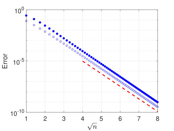
In Figure 5 we plot the errors of Gauss–Hermite quadrature $Q_{n}^{\mathrm{GH}}(f)$ for the functions

$$f(x)=\frac{1}{\sqrt{1+x^{2}}},\qquad\frac{e^{-x^{2}}}{\sqrt{1+x^{2}}}.$$

It is easily seen that both functions have branch singularities at $\pm\mathrm{i}$, and therefore, by Theorem 5.1, the associated rates of convergence of Gauss–Hermite quadrature rule are $O(\exp(-2\sqrt{2n}))$. We can see from Figure 5 that the actual rate of convergence of Gauss–Hermite quadrature is consistent with our theoretical result.

Figure 5: The error of $Q_{n}^{\mathrm{GH}}(f)$ as a function of $\sqrt{n}$ for $f(x)=1/\sqrt{1+x^{2}}$ (circles) and $f(x)=e^{-x^{2}}/\sqrt{1+x^{2}}$ (dots). The dashed line shows the predicted rate $O(\exp(-2\sqrt{2n}))$.

Remark 5.2.

Gaussian quadrature rules are known to be optimal in the sense that they achieve the highest algebraic degree of exactness. However, as pointed out recently by Trefethen in [28], this exactness principle for Gauss–Hermite quadrature might be suboptimal since most of the quadrature nodes are far from the origin and the corresponding quadrature weights lie below the machine precision and thus contribute negligibly to the result of Gauss–Hermite quadrature. We refer to [16] for further investigations of this suboptimality for functions with finite smoothness.

5.2 Hermite spectral differentiations

We have established the convergence rate for Hermite projections in Theorems 3.4 and 3.6. It comes out that we could further extend the analysis to Hermite spectral differentiations.

Theorem 5.3.

Let $\Pi_{n}^{\mathrm{P}}f$ and $\Pi_{n}^{\mathrm{F}}f$ be defined in (3.3) and (3.16), respectively, and let $m\in\mathbb{N}$. For $n\gg 1$, the following statements are true.

• Under the assumptions of Theorem 3.1, we have

  $$\|(f-\Pi_{n}^{\mathrm{P}}f)^{(m)}\|_{L_{\omega}^{2}(\mathbb{R})}\leq\mathcal{K}n^{m/2}e^{-\rho\sqrt{2n}},$$ (5.4)

  where $\mathcal{K}\approx 2^{m/2-1}V/\sqrt{\pi\rho}$ with $V$ given in (3.8).

• Under the assumptions of Theorem 3.6, we have

  $$\|(f-\Pi_{n}^{\mathrm{F}}f)^{(m)}\|_{L^{\infty}(\mathbb{R})}\leq\mathcal{K}n^{m/2+1/4}e^{-\rho\sqrt{2n}},$$ (5.5)

  where $\mathcal{K}\approx 2^{m/2-1/4}\widehat{V}/\pi^{3/4}$ with $\widehat{V}$ given in (3.17).

Proof.

By [19, Equation (18.9.25)], it follows that

$$\frac{\mathrm{d}^{m}}{\mathrm{d}x^{m}}H_{k}(x)=\frac{2^{m}\Gamma(k+1)}{\Gamma(k-m+1)}H_{k-m}(x),\qquad k\geq m.$$

Thus, by Theorem 3.4, the duplication formula and ratio asymptotics for the gamma function (see [19, Equations (5.5.5) and (5.11.13)]), we have, for $n\gg 1$,

$$\|(f-\Pi_{n}^{\mathrm{P}}f)^{(m)}\|_{L_{\omega}^{2}(\mathbb{R})}^{2} =\sum_{k=n+1}^{\infty}a_{k}^{2}\left(\frac{2^{m}\Gamma(k+1)}{\Gamma(k-m+1)}\right)^{2}\gamma_{k-m}$$

$$\leq\mathcal{K}^{2}\frac{2^{m-3/2}}{\pi}\sum_{k=n+1}^{\infty}k^{m-1/2}e^{-2\rho\sqrt{2k}}$$

$$\leq\mathcal{K}^{2}\frac{2^{m-3/2}}{\pi}\int_{n}^{\infty}x^{m-1/2}e^{-2\rho\sqrt{2x}}\mathrm{d}x$$

$$=\mathcal{K}^{2}\frac{\Gamma(2m+1,2\rho\sqrt{2n})}{2\pi(2\rho)^{2m+1}},$$

where $\mathcal{K}\approx V$. The desired estimate (5.4) follows from combining the last bound with the fact $\Gamma(a,z)=z^{a-1}e^{-z}(1+O(z^{-1}))$ as $z\to\infty$ (see [19, Equation (8.11.2)]).

As for (5.5), by (2.4) and [19, Equation (18.9.25)], we find that

$$\frac{\mathrm{d}}{\mathrm{d}x}\psi_{n}(x) =\sqrt{\frac{n}{2}}\psi_{n-1}(x)-\sqrt{\frac{n+1}{2}}\psi_{n+1}(x).$$

By repeated application of this equation and the inequality (3.15), it is easily verified that $\|\psi_{n}^{(m)}\|_{L^{\infty}(\mathbb{R})}\leq\mathcal{K}n^{m/2}$, where $\mathcal{K}\approx 2^{m/2}/\pi^{1/4}$ for $n\gg 1$. Combining this with Theorem 3.6, we deduce that

$$\|(f-\Pi_{n}^{\mathrm{F}}f)^{(m)}\|_{L^{\infty}(\mathbb{R})} \leq\sum_{k=n+1}^{\infty}|c_{k}|\|\psi_{k}^{(m)}\|_{L^{\infty}(\mathbb{R})}\leq\mathcal{K}\sum_{k=n+1}^{\infty}k^{m/2-1/4}e^{-\rho\sqrt{2k}},$$

where $\mathcal{K}\approx 2^{m/2-3/4}\widehat{V}/\pi^{3/4}$. The remaining steps are similar to the case of $\Pi_{n}^{\mathrm{P}}f$ and we omit the details. This ends the proof. ∎

5.3 Generalized Hermite spectral approximations

Generalized Hermite polynomials, which were introduced by Szegő in his monograph [24, p. 380], are also of interest in practice (see, e.g., [21, 23]). These polynomials are orthogonal with respect to the weight function

$$\omega_{\mu}(x):=|x|^{2\mu}e^{-x^{2}},\qquad\mu>-\frac{1}{2},$$ (5.6)

over the real axis. For convenience, we consider the monic polynomials $\pi_{n}^{(\mu)}(x)=x^{n}+\cdots$, which are characterized by the orthogonality conditions

$$\langle\pi_{n}^{(\mu)},\pi_{m}^{(\mu)}\rangle_{\omega_{\mu}}=\gamma_{n}^{(\mu)}\delta_{n,m},\quad n,m\in\mathbb{N}_{0};$$ (5.7)

see also [21] for the explicit formulas of a suitably normalized set of generalized Hermite polynomials.

As can be seen from our previous analysis, a key ingredient in the present case will be the large $n$ asymptotics of the weighted Cauchy transform of the generalized Hermite polynomials defined by

$$\Phi_{n}^{(\mu)}(z)=\frac{1}{2\pi\mathrm{i}}\int_{\mathbb{R}}\frac{\omega_{\mu}(x)\pi_{n}^{(\mu)}(x)}{z-x}\mathrm{d}x,\quad z\in\mathbb{C}\setminus\mathbb{R},$$ (5.8)

In contrast to (2.11), it is still unknown how to express $\Phi_{n}^{(\mu)}(z)$ explicitly via some classical special functions. Nevertheless, it is still possible to find the asymptotics of $\Phi_{n}^{(\mu)}$ by using the Riemann-Hilbert (RH) approach [8]. Let

$$Y_{n}(z):=\begin{pmatrix}\pi_{n}^{(\mu)}(z)&\Phi_{n}^{(\mu)}(z)\\[8.61108pt] \kappa_{n}^{(\mu)}\pi_{n-1}^{(\mu)}(z)&\kappa_{n}^{(\mu)}\Phi_{n-1}^{(\mu)}(z)\end{pmatrix},\quad\kappa_{n}^{(\mu)}=-\frac{2\pi\mathrm{i}}{\gamma_{n-1}^{(\mu)}},$$

where $\gamma_{n}^{(\mu)}$ is given in (5.7). By [11], it is well-known that $Y_{n}$ is the unique solution of the following RH problem:

1. $Y_{n}(z)$ is analytic in $\mathbb{C}\setminus\mathbb{R}$.

2. $Y_{n}(z)$ takes continuous boundary values $Y_{n,+}(x)$ and $Y_{n,-}(x)$ such that

   $$Y_{n,+}(x)=Y_{n,-}(x)\begin{pmatrix}1&\omega_{\mu}(x)\\ 0&1\end{pmatrix},\qquad x\in\mathbb{R}\setminus\{0\},$$

   where $\omega_{\mu}$ is the weight function given in (5.6) and the orientation of $\mathbb{R}$ is taken from the left to the right.

3. As $z\to\infty$ and $z\in\mathbb{C}\setminus\mathbb{R}$, we have

   $$Y_{n}(z)=(I+O(1/z))\begin{pmatrix}z^{n}&0\\ 0&z^{-n}\end{pmatrix},$$

   where $I$ stands for the $2\times 2$ identity matrix.

4. As $z\to 0$ and $z\in\mathbb{C}\setminus\mathbb{R}$, we have

   $$Y_{n}(z)=\begin{cases}O\begin{pmatrix}1&|z|^{2\mu}\\ 1&|z|^{2\mu}\end{pmatrix},\quad&\textrm{$\mu<0$},\\[12.91663pt] O\begin{pmatrix}1&\ln|z|\\ 1&\ln|z|\end{pmatrix},\quad&\textrm{$\mu=0$},\\[12.91663pt] O\begin{pmatrix}1&1\\ 1&1\end{pmatrix},\quad&\textrm{$\mu>0$}.\end{cases}$$

Note that the $(1,2)$-entry of $Y_{n}$ is exactly the weighted Cauchy transform of the generalized Hermite polynomials, one can then extract the asymptotics of $\Phi_{n}^{(\mu)}(z)$ by performing a Deift-Zhou nonlinear steepest descent analysis [7, 8] to the RH problem for $Y_{n}$. This analysis consists of a series of explicit transformations in such a way that each transformation simplifies the nature of the subsequent one and the final goal is to arrive at an RH problem tending to the identity matrix as $n\to\infty$. Unraveling all the transformations leads to the desired asymptotics. For the weight function $\omega_{\mu}$ in (5.6), this analysis can be found in [34], although the emphasis therein is on the orthogonal polynomials $\pi_{n}^{(\mu)}$. Thus, from [34], we have, as $n\to\infty$,

$$\Phi_{n}^{(\mu)}(\sqrt{N}z)=\frac{\textrm{i}N^{(N+\mu)/2}}{2}z^{\mu}e^{N(\ell-g(z))}\left(a(z)^{-1}-a(z)\right)\left(1+O(N^{-1})\right),$$ (5.9)

where $z\in\mathbb{C}\setminus\mathbb{R}$, $N:=n+\mu$, $\ell:=-1-\log 2$, and

$$g(z): =\frac{1}{\pi}\int_{-\sqrt{2}}^{\sqrt{2}}\log(z-x)\sqrt{2-x^{2}}\mathrm{d}x,$$

$$=\frac{z^{2}+\ell}{2}-2\int_{1}^{z/\sqrt{2}}(t^{2}-1)^{1/2}\mathrm{d}t,\qquad z\in\mathbb{C}\setminus(-\infty,\sqrt{2}],$$

$$a(z): =\left(\frac{z-\sqrt{2}}{z+\sqrt{2}}\right)^{1/4},\quad z\in\mathbb{C}\setminus[-\sqrt{2},\sqrt{2}],$$

and the error bound is uniformly valid for any compact subset of $\mathbb{C}\setminus\mathbb{R}$. Note that, as $z\to 0$, it is readily seen that for $\pm\Im z>0$,

$$g(z)=\frac{\ell}{2}\mp\frac{\pi\textrm{i}}{2}\mp\sqrt{2}\textrm{i}z+\frac{z^{2}}{2}+O(z^{3}),\quad a(z)^{-1}-a(z)=\mp\sqrt{2}\textrm{i}+O(z).$$

Hence, by replacing $z$ in (5.9) by $z/\sqrt{N}$, it follows from the above two expansions that as $n\to\infty$,

$$|\Phi_{n}^{(\mu)}(z)| =\frac{1}{\sqrt{2}}\left(\frac{N}{2}\right)^{\frac{N}{2}}e^{-\frac{N}{2}}|z|^{\mu}|e^{-z^{2}/2}|e^{-|\Im(z)|\sqrt{2N}}\left(1+O(N^{-1/2})\right),$$ (5.10)

for $z\in\mathbb{C}\setminus\mathbb{R}$, which matches with the leading term of the asymptotic expansion of (2.12) if $\mu=0$.

A combination of the above asymptotic formula and the strategy proposed for Hermite spectral approximations implies that one should also obtain the root-exponential convergence rate of generalized Hermite spectral approximations for analytic functions. We leave the details to interested readers.

5.4 The scaling factor of Hermite approximation

In practice, it is common to use the scaled Hermite functions as the basis functions in order to accelerate the rate of convergence; cf. [4, 25]. More precisely, given a function $f$, we consider the Hermite approximation of the form

$$f_{n,\lambda}^{\mathrm{SF}}(x)=\sum_{k=0}^{n}\alpha_{k}\psi_{k}(\lambda x),\qquad\alpha_{k}=\lambda\int_{\mathbb{R}}f(x)\psi_{k}(\lambda x)\mathrm{d}x,$$ (5.11)

where $\psi_{k}$ is the Hermite function defined in (3.13) and $\lambda>0$ is a scaling factor.

It comes out that our convergence analysis is also helpful to some extent in finding the scaling factor. If $f(z)$ is analytic inside and on the infinite strip $\mathcal{S}_{\rho}$ for some $\rho>0$ and $|e^{z^{2}/2}f(z/\lambda)|\leq\mathcal{K}|z|^{\sigma}$ for some $\sigma\in\mathbb{R}$ as $|z|\to\infty$ within the strip $\mathcal{S}_{\lambda\rho}$, we then obtain from Theorem 3.6 that $f_{n,\lambda}^{\mathrm{SF}}(x)$ converges at the rate $O(n^{1/4}\exp(-\lambda\rho\sqrt{2n}))$ in the maximum norm. Clearly, the scaling factor $\lambda$ in this case should be chosen as large as possible to maximize the convergence rate. As an example, we consider the function $f(x)=e^{-2x^{2}}/(1+x^{2})$, which has a pair of conjugate simple poles at $z=\pm\mathrm{i}$. Our analysis implies that the convergence rate of $f_{n,\lambda}^{\mathrm{SF}}(x)$ in the maximum norm is $O(n^{1/4}\exp(-\lambda\sqrt{2n}))$ whenever $\lambda\leq 2$. In the left panel of Figure 6 we plot the maximum errors of $f_{n,\lambda}^{\mathrm{SF}}(x)$ for three different values of $\lambda\leq 2$. As expected, the convergence rate of $f_{n,\lambda}^{\mathrm{SF}}(x)$ is indeed $O(n^{1/4}\exp(-\lambda\sqrt{2n}))$ and the choice of $\lambda=2$ achieves faster convergence rate than $\lambda=1$. Nevertheless, we point out that $\lambda=2$ is still not the optimal scaling factor. Indeed, in the right panel of Figure 6 we plot the maximum errors of $f_{n,\lambda}^{\mathrm{SF}}(x)$ for three greater values of $\lambda$. We can see that the choice $\lambda=5/2$ achieves faster convergence rate than $\lambda=2$, which is actually faster than root-exponential rate.

Figure 6: The maximum error of $f_{n,\lambda}^{\mathrm{SF}}(x)$ as a function of $\sqrt{n}$ for several different scaling factors. The dashed lines in the left panel show the predicted rates $O(n^{1/4}\exp(-\lambda\sqrt{2n}))$.

6 Conclusion

In this work we have presented a rigorous convergence analysis of Hermite spectral approximations for functions that are analytic within and on an infinite strip and satisfies certain restrictions on the asymptotic behavior at infinity within the strip. By exploring some remarkable contour integral representations for the Hermite coefficients and the remainder of Hermite spectral approximations, we derive some asymptotically sharp error bounds for Hermite approximations in the weighted and maximum norms. Extensions of our analysis to Gauss–Hermite quadrature, Hermite spectral differentiations, generalized Hermite spectral approximations and the scaling factor of Hermite approximation are also discussed.

Finally, we emphasize that our analysis for Hermite expansions here is different from that conducted in [3]. Note that our analysis is based on the contour integral representation of Hermite coefficients with which some precise bounds on Hermite coefficients can be derived, but the analysis in [3] relies on the method of steepest descent, which can only give some asymptotic estimates for Hermite coefficients. However, some issues related to our analysis still remain. For example, our analysis for Hermite approximations using $\{\psi_{k}\}$ requires a strong condition on the asymptotic behavior of the underlying functions at infinity, which excludes some classes of analytic functions. It is then unclear whether the condition can be further relaxed. Moreover, Figure 6 implies that the choice of the optimal scaling factor still does not follow from our convergence analysis. We leave theses issues for future research.

References

• [1] W. Barrett, Convergence properties of Gaussian quadrature formulae, Comput. J., 3(4):272–277, 1961.
• [2] J. P. Boyd, The rate of convergence of Hermite function series, Math. Comp., 35(152):1309–1316, 1980.
• [3] J. P. Boyd, Asymptotic coefficients of Hermite function series, J. Comput. Phys., 54(3):382–410, 1984.
• [4] J. P. Boyd, Chebyshev and Fourier Spectral Methods, Dover Publications, Inc., New York, 2000.
• [5] C. Canuto, M. Y. Hussaini, A. Quarteroni and T. A. Zang, Spectral Methods: Fundamentals in Single Domains, Springer-Verlag, Berlin, 2006.
• [6] P. J. Davis, Interpolation and Approximation, Dover Publications, New York, 1975.
• [7] P. Deift, Orthogonal Polynomials and Random Matrices: A Riemann-Hilbert Approach, Courant Lecture Notes, vol. 3, New York University, 1999.
• [8] P. Deift and X. Zhou, A steepest descent method for oscillatory Riemann-Hilbert problems. Asymptotics for the MKdV equation, Ann. Math., 137(2):295–368, 1993.
• [9] J. D. Donaldson and D. Elliott, A unified approach to quadrature rules with asymptotic estimates of their remainders, SIAM J. Numer. Anal., 9(4):573–602, 1972.
• [10] D. Elliott and P. D. Tuan, Asymptotic estimates of Fourier coefficients, SIAM J. Math. Anal., 5(1):1–10, 1974.
• [11] A. S. Fokas, A. R. Its and A. V. Kitaev, The isomonodromy approach to matrix models in $2$D quantum gravity, Comm. Math. Phys., 147(2):395–430, 1992.
• [12] E. Hille, Contributions to the theory of Hermitian series, Duke Math. J., 5(4):875–936, 1939.
• [13] E. Hille, Contributions to the theory of Hermitian series II. The representation problem, Trans. Amer. Math. Soc., 47(1):80–94, 1940.
• [14] A. Iserles and M. Webb, Orthogonal systems with a skew-symmetric differentiation matrix, Found. Comput. Math., 19(6):1191–1221, 2019.
• [15] M. E. H. Ismail, Classical and Quantum Orthogonal Polynomials in One Variable, Cambridge University Press, Cambridge, 2005.
• [16] Y. Kazashi, Y. Suzuki and T. Goda, Suboptimality of Gauss–Hermite quadrature and optimality of the trapezoidal rule for functions with finite smoothness, SIAM J. Numer. Anal., 61(3):1426–1448, 2023.
• [17] Z.-P. Mao and J. Shen, Hermite spectral methods for fractional PDEs in unbounded domain, SIAM J. Sci. Comput., 39(5):A1928–A1950, 2017.
• [18] N. I. Muskhelishvili, Singular Integral Equations: Boundary problems of functions theory and their applications to mathematical physics, Wolters-Noordhoff Publishing, Groningen, 1972.
• [19] F. W. J. Olver, D. W. Lozier, R. F. Boisvert and C. W. Clark, NIST Handbook of Mathematical Functions, Cambridge University Press, Cambridge, 2010.
• [20] S. C. Reddy and J. A. C. Weideman, The accuracy of the Chebyshev differencing method for analytic functions, SIAM J. Numer. Anal., 42(5):2176–2187, 2005.
• [21] M. Rosenblum, Generalized Hermite polynomials and the Bose-like oscillator calculus, Operator Theory: Advances and Applications, 73:369–396, Birkhauser-Verlag, Basel, 1994.
• [22] J. Shen, T. Tang and L.-L. Wang, Spectral Methods: Algorithms, Analysis and Applications, Springer, Heidelberg, 2011.
• [23] C.-T. Sheng, S.-N. Ma, H.-Y. Li, L.-L. Wang and L.-L. Jia, Nontensorial generalised Hermite spectral methods for PDEs with fractional Laplacian and Schrödinger operators, ESAIM: M2AN, 55(5):2141–2168, 2021.
• [24] G. Szegő, Orthogonal Polynomials, American Mathematical Society Colloquium Publications, vol. 23, New York, 1939.
• [25] T. Tang, The Hermite spectral method for Gaussian-type functions, SIAM J. Sci. Comput., 14(3):594–606, 1993.
• [26] N. M. Temme, Asymptotic methods for integrals, volume 6 of Series in Analysis, World Scientific Publishing Co. Pte. Ltd., Hackensack, NJ, 2015.
• [27] N. M. Temme, On the expansion of confluent hypergeometric functions in terms of Bessel functions, J. Comput. Appl. Math., 7(1):27–32, 1981.
• [28] L. N. Trefethen, Exactness of quadrature formulas, SIAM Rev., 64(1):132–150, 2022.
• [29] H.-Y. Wang and S.-H. Xiang, On the convergence rates of Legendre approximation, Math. Comp., 81(278):861–877, 2012.
• [30] H.-Y. Wang, How much faster does the best polynomial approximation converge than Legendre projection?, Numer. Math., 147(2):481–503, 2021.
• [31] H.-Y. Wang, Optimal rates of convergence and error localization of Gegenbauer projections, IMA J. Numer. Anal., 43(4):2413–2444, 2023.
• [32] H.-Y. Wang, Optimal convergence analysis of Laguerre spectral approximations for analytic functions, arXiv:2304.05744, 2023.
• [33] L.-L. Wang, X.-D. Zhao and Z.-M. Zhang, Superconvergence of Jacobi–Gauss–type spectral interpolation, J. Sci. Comput., 59(3):667–687, 2014.
• [34] R. Wong and L. Zhang, Global asymptotics of orthogonal polynomials associated with $|x|^{2\alpha}e^{-Q(x)}$, J. Approx. Theory, 162(4):723–765, 2010.
• [35] J. A. C. Weideman, The eigenvalues of Hermite and rational spectral differentiation matrices, Numer. Math., 61(3):409–431, 1992.
• [36] S.-H. Xiang, On error bounds for orthogonal polynomial expansions and Gauss–type quadrature, SIAM J. Numer. Anal., 50(3):1240–1263, 2012.
• [37] S.-H. Xiang, Asymptotics on Laguerre or Hermite polynomial expansions and their applications in Gauss quadrature, J. Math. Anal. Appl., 393(2):434–444, 2012.
• [38] Z.-Q. Xie, L.-L. Wang and X.-D. Zhao, On exponential convergence of Gegenbauer interpolation and spectral differentiation, Math. Comp., 82(282):1017–1036, 2013.
• [39] X.-D. Zhao, L.-L. Wang and Z.-Q. Xie, Sharp error bounds for Jacobi expansions and Gegenbauer-Gauss quadrature of analytic functions, SIAM J. Numer. Anal., 51(3):1443–1469, 2013.